A study of perturbations in scalar–tensor theory using 1 + 3 covariant approach

Joseph Ntahompagaze^1,2,4, Amare Abebe^2,1,3 and Manasse R. Mbonye⁴

Email: ntahompagazej@gmail.com,  amare.abbebe@gmail.com,  mmbonye@gmail.com

¹ Astronomy and Astrophysics Division, Entoto Observatory and Research Center, Ethiopia
² Department of Physics, North-West University, South Africa
³ Center for Space Research, North-West University, South Africa
⁴ Department of Physics, College of Science and Technology, University of Rwanda, Rwanda

Abstract

This work discusses scalar-tensor theories of gravity, with a focus on the Brans-Dicke sub-class, and one that also takes note of the latter’s equivalence with $f(R)$ gravitation theories. A $1+3$ covariant formalism is used in this case to discuss covariant perturbations on a background Friedmann-Laimaître-Robertson-Walker (FLRW) space-time. Linear perturbation equations are developed, based on gauge-invariant gradient variables. Both scalar and harmonic decompositions are applied to obtain second-order equations. These equations can then be used for further analysis of the behavior of the perturbation quantities in such a scalar-tensor theory of gravitation. Energy density perturbations are studied for two systems, namely for a scalar fluid-radiation system and for a scalar fluid-dust system, for $R^{n}$ models. For the matter-dominated era, it is shown that the dust energy density perturbations grow exponentially, a result which agrees with those already in existing literature. In the radiation-dominated era, it is found that the behavior of the radiation energy-density perturbations is oscillatory, with growing amplitudes for $n>1$, and with decaying amplitudes for $0<n<1$. This is a new result.

$keywords:$ $f(R)$ gravity – scalar-tensor –scalar field –cosmology –covariant perturbation.
$PACSnumbers:$ 04.50.Kd, 98.80.-k, 95.36.+x, 98.80.Cq;
$MSCnumbers:$ 83Dxx, 83Fxx, 83Cxx

1 Introduction

Scalar-tensor theories have been widely explored [1, 2, 3, 4] and their relationship with $f(R)$ gravity theories are discussed [5, 6, 7]. Recent focus [8, 9, 10, 11, 12, 13] has been on the $f(R)$ theories as a special class of Brans-Dicke scalar-tensor theories. In the current work we continue to explore this relationship following on our recent work [11]. In particular, we apply a $1+3$ covariant formalism to study cosmological perturbations. This formalism was introduced by Ellis and Bruni in the 1980s [14, 15]. This approach is constructed in such a way that the spacetime four-dimensional manifold is split into a 3-dimensional sub-manifold perpendicular to a time-like vector field. This formalism has advantage that the quantities defined have both geometrical and physical meaning and they can be measured. In [16], the authors showed the importance of gauge-invariant gradient variables and their physical meaning. In cosmology, perturbations of several quantities like the energy density parameter, expansion parameter and those of curvature have previously been treated. The $1+3$ covariant formalism has been applied to study linear perturbation in General Relativity [15]. The same studies has been done in $f(R)$ gravity at linear order and results have been obtained [17, 18]. In scalar-tensor theory, the $1+3$ covariant linear perturbation has been studied [19, 20], but it was limited to vacuum case. The assumption that the hyper-surfaces are with constant scalar field was made in that study. Those hyper-surfaces are perpendicular to a vector field.

In this paper, we consider hyper-surfaces with constant curvature. They have been considered for $f(R)$ covariant perturbations [18, 17, 21]. This consideration is taken due to the equivalence between metric $f(R)$ theory of gravity and Brans-Dicke scalar-tensor theory. The equivalence between $f(R)$ gravity and scalar-tensor theory in five dimensions have been considered in [7, 22], where Jordan frame was given much attention and bulk consideration which resulted in hyper-surfaces of four dimensional space-times. In our study, the hyper-surfaces are constructed from $1+3$ covariant decomposition of spacetime such that they have three dimensions. The work presented in this paper is a follow-up of the work previously done by the authors [11], where the equivalence between $f(R)$ theory and scalar-tensor theory has been explored. Here, this equivalence is extended to covariant linear perturbations for two fluid system with the consideration that scalar field behaves like a fluid (scalar fluid). The two fluid system (radiation-scalar field or dust-scalar field) are considered with the motivation that towards the end of a scalar field driven inflation the universe experienced a mixture of scalar field and radiation. Later during the matter dominated epoch one can think of a situation where the scalar field was so small that its effect becomes less significant.

This paper is organized as follows: in the next section, the $1+3$ covariant formalism is described. In Section 3, the equivalence between $f(R)$ and scalar tensor theories of gravitation is reviewed. In Section 4, background evolution equations for the FLRW universe are provided to play a ground for the coming perturbation equations. Section 5 is for definition of gradient variables to be used in evolution equations. The next two sections are for linear and scalar evolution equations. In Section 8, we perform harmonic decomposition to make equations simpler where partial differential equations are reduced ordinary differential equations. In Section 9, we apply perturbations to scalar field dominated universe and two different cases have been considered; namely scalar field-dust system and scalar field-radiation system. Finally, the conclusion is drawn in Section 10. The adopted spacetime signature is $(-+++)$ and unless stated otherwise, we have used the convention $8\pi G=c=1$, where $G$ is the gravitational constant and $c$ is the speed of light.

2 1+3 covariant approach for scalar-tensor theories

The $1+3$ covariant approach divides space-time into foliated hyper-surfaces and a perpendicular 4-vector-field. In this process, the cosmological manifold $(\mathcal{M},g)$ is decomposed into the sub-manifold $(M,h)$ which has a perpendicular 4-velocity field vector $u^{a}$ [14, 15]. The background under consideration is the FLRW spacetime with a scalar field $\phi$. Note that these hypersurfaces are spacelike. The 4-velocity field vector $u^{a}$ is defined as

$$u^{a}=\frac{dx^{a}}{d\tau}\;,$$ (1)

where $\tau$ is proper time such that $u_{a}u^{a}=-1.$ This approach helps in the decomposition of the metric $g_{ab}$ into the projection tensor $h_{ab}$ as [21, 23]:

$$g_{ab}=h_{ab}-u_{a}u_{b}\;.$$ (2)

Here the projection tensors (parallel $U^{a}_{b}$ and orthogonal $h_{ab}$) are defined as

$$U^{a}_{b}=-u^{a}u_{b}\Rightarrow U^{a}_{c}U^{c}_{b}=U^{a}_{b},\;U^{a}_{a}=1,\;U_{ab}u^{b}=u_{a}\;,$$ (3)

and

$$h_{ab}=g_{ab}+u_{a}u_{b}\Rightarrow h^{a}_{c}h^{c}_{b}=h^{a}_{b},\;h^{a}_{a}=3,\;h_{ab}u^{b}=0\;.$$ (4)

The projection tensor $U^{a}_{b}$ projects parallel to the 4-velocity vector $u^{a}$ and the $h_{ab}$ is responsible for the metric properties of instantaneous rest-spaces of observers moving perpendicularly with 4-velocity $u^{a}$. The derivatives also follow with respect to those projectors. The covariant time derivative (for a given tensor $T^{ab}_{cd}$) is given as

$$\dot{T}^{ab}_{cd}=u^{e}\nabla_{e}T^{ab}_{cd}\;.$$ (5)

In this approach, the kinematic quantities which are obtained from irreducible parts of the decomposed $\nabla_{a}u_{b}$ are given as [23]

$$\nabla_{a}u_{b}=\tilde{\nabla}_{a}u_{b}-u_{a}\dot{u}_{b}=\frac{1}{3}\Theta h_{ab}+\sigma_{ab}+\omega_{ab}-u_{a}\dot{u}_{b}\;,$$ (6)

where $\tilde{\nabla}$ refers to a 3-spatial gradient, the volume rate of expansion of the fluid $\Theta=\tilde{\nabla}_{a}u^{a}$, the Hubble parameter $H=\frac{\Theta}{3}=\frac{\dot{a}}{a}$, the rate of distortion of the matter flow $\sigma_{ab}=\tilde{\nabla}_{<a}u_{b>}$, is the trace-free symmetric rate of the shear tensor $(\sigma_{ab}=\sigma_{(ab)},\sigma_{ab}u^{b}=0,\sigma^{a}_{a}=0)$. The vorticity tensor $\omega_{ab}=\tilde{\nabla}_{[a}u_{b]}$ is the skew-symmetric vorticity tensor and describes the rotation of the matter relative to a non-rotating frame. The relativistic acceleration vector (not that of the expansion of the universe) is given as $\dot{u}^{a}=u^{b}\nabla_{b}u^{a}$. These kinematic quantities provide informations about the overall spacetime kinematics. We define also the volume element for 3-restspace as

$$\eta_{abc}=u^{d}\eta_{abcd},\text{ }\eta_{abc}=\eta_{[abc]},\text{ }\eta_{abc}u^{c}=0\;,$$ (7)

where $\eta_{abcd}$ is a 4-dimensional volume element. The matter energy-momentum tensor $T_{ab}$ is also decomposed with the 1+3 covariant approach and it is given as [17, 23]

$$T_{ab}=\mu u_{a}u_{b}+q_{a}u_{b}+u_{a}q_{b}+ph_{ab}+\pi_{ab}\;,$$ (8)

where $\mu$ is the relativistic energy density, $q^{a}$ is the relativistic momentum density (energy flux relative to $u^{a}$), $p$ is relativistic isotropic pressure, and $\pi_{ab}$ is the trace-free anisotropic pressure of the fluid ($\pi^{a}_{a}=0,\pi_{ab}=\pi_{(ab)},\pi_{ab}u^{b}=0$). The energy-momentum tensor for the perfect fluid can be recovered by setting ($q^{a}=\pi_{ab}=0$) and that tensor $T_{ab}$ reads

$$T_{ab}=\mu u_{a}u_{b}+ph_{ab}\;,$$ (9)

where the equation of state for perfect fluid is $p=p(\mu)$.

3 $f(R)$ theory in scalar-tensor language

Let us consider the action that represents $f(R)$ gravity given as

$$I=\frac{1}{2\kappa}\int d^{4}x\sqrt{-g}\left[f(R)+2\mathcal{L}_{m}\right]\;,$$ (10)

where $\kappa=8\pi G$,$R$ is Ricci scalar and $\mathcal{L}_{m}$ is the matter Lagrangian. The action in scalar-tensor theory has the form [8, 5]

$$I_{f(\phi)}=\frac{1}{2\kappa}\int d^{4}\sqrt{-g}\left[f(\phi)+2\mathcal{L}_{m}\right]\;,$$ (11)

where $f(\phi)$ is the function of $\phi(R)$ and specifically where we define the scalar field $\phi$ to be [8, 11] of the form

$$\phi=f^{\prime}-1\;,$$ (12)

where for GR, we have a vanishing scalar field. Here the prime indicates differentiation with respect to $R$ and we require that the scalar field $\phi$ be invertible [6, 5, 24]. The field equations from the action in Eq. (11) are given in [5] as:

$$G_{ab}=\frac{\kappa}{\phi+1}T^{m}_{ab}+\frac{1}{(\phi+1)}\left[\frac{1}{2}g_{ab}\Big{(}f-(\phi+1)R\Big{)}+\nabla_{a}\nabla_{b}\phi-g_{ab}\square\phi\right]\;,$$ (13)

where $\square=\nabla_{c}\nabla^{c}$ is the covariant D’Alembert operator and $T^{m}_{ab}$ is the matter energy-momentum tensor. The scalar field $\phi$ obeys the Klein-Gordon equation [8]

$$\square\phi-\frac{1}{3}\Big{(}2f-(\phi+1)R+T^{m}\Big{)}=0\;,$$ (14)

where $T^{m}$ is the trace of the matter energy momentum tensor.
One can consider at this stage the Friedmann and Rychaudhuri equations given as

$$\Theta^{2}=3(\overline{\mu}_{m}+\mu_{\phi})-\frac{9K}{a^{2}}\;,$$ (15)

and

$$\dot{\Theta}+\frac{1}{3}\Theta^{2}+\frac{1+3w}{2}\overline{\mu}_{m}+\frac{1}{2}(\mu_{\phi}+3p_{\phi})=0\;,$$ (16)

where $w$ is equation of state parameter (EoS), $\mu_{\phi}$ is the energy density and $p_{\phi}$ is isotropic pressure of scalar fluid respectively; $K$ stands for curvature and has the values $0,-1,+1$ for flat, open and closed universe respectively, $a$ is the scale factor and $\overline{\mu}_{m}=\frac{\mu_{m}}{\phi+1}$. For the flat $(K=0)$ FLRW background one has Ricci scalar given as

$$R=6\Big{(}\frac{\ddot{a}}{a}+\frac{\dot{a}^{2}}{a^{2}}\Big{)}\;.$$ (17)

4 Background (zeroth-order) quantities

Now since the background is considered to be the FLRW spacetime, the background quantities: energy density and isotropic pressure for the curvature fluid are given as [21]

$$\mu_{R}=\frac{1}{f^{\prime}}\Big{[}\frac{1}{2}(Rf^{\prime}-f)-\Theta f^{\prime\prime}\dot{R}\Big{]}$$ (18)

$$p_{R}=\frac{1}{f^{\prime}}\Big{[}\frac{1}{2}(f-Rf^{\prime})+f^{\prime\prime}\ddot{R}+f^{\prime\prime\prime}\dot{R}^{2}+\frac{2}{3}\Theta f^{\prime\prime}\dot{R}\Big{]}\;.$$ (19)

Analogously, we have energy density and pressure for scalar fluid as

$$\mu_{\phi}=\frac{1}{\phi+1}\left[\frac{1}{2}\Big{(}(\phi+1)R-f\Big{)}-\Theta\dot{\phi}\right]\;,$$ (20)

$$p_{\phi}=\frac{1}{\phi+1}\left[\frac{1}{2}\Big{(}f-R(\phi+1)\Big{)}+\ddot{\phi}-\frac{\dot{\phi}\dot{\phi}^{\prime}}{\phi^{\prime}}\phi^{\prime\prime}+\frac{\phi^{\prime\prime}\dot{\phi}^{2}}{\phi^{\prime 2}}+\frac{2}{3}\Theta\dot{\phi}\right]\;.$$ (21)

For FLRW spacetime, the kinematic quantities presented in Eq. (6) satisfy

$$\sigma_{ab}=0,\text{ }\omega_{a}=0,\text{ }\dot{u}_{a}=0,\text{ }\tilde{\nabla}_{a}\Theta=0\;.$$ (22)

Also for any scalar quantity $f$, in the background we have

$$\tilde{\nabla}_{a}f=0,$$ (23)

and hence, at the background

$$\tilde{\nabla}_{a}\mu=0,\text{ }\tilde{\nabla}_{a}p=0,\text{ }\tilde{\nabla}_{a}\phi=0\;,$$ (24)

and

$$q^{\phi}_{a}=\pi^{\phi}_{ab}=0\;.$$ (25)

The energy conservation or simply the continuity equations for matter and scalar field fluid are given as

$$\dot{\mu}_{m}=-\Theta(\mu_{m}+p_{m})\;,$$ (26)

$$\dot{\mu}_{\phi}=-\Theta(\mu_{\phi}+p_{\phi})+\frac{\dot{\phi}\mu_{m}}{(\phi+1)^{2}}\;.$$ (27)

One can easily notice the coupling between these two equations from matter energy density in the last term of equation (27) where $\mu_{m}$ is present as a factor.

5 Definition of gradient variables

Gauge-invariant quantities are key for the cosmological perturbations analysis. A quantity is said to be gauge-invariant (GI), (Stewart-Walker Lemma [21, 25]) if it vanishes in the background. We define GIs in 1+3 covariant perturbations in the following way. The GI variable that characterizes energy density perturbation in spatial variation is given as [18, 21, 26, 27]

$$X_{a}=\tilde{\nabla}_{a}\mu\;.$$ (28)

Then from this quantity, we can define the following GI variable

$$D_{a}=\frac{a}{\mu}X_{a}=\frac{a}{\mu}\tilde{\nabla}_{a}\mu\;.$$ (29)

The ratio $\frac{a}{\mu}$ helps to evaluate the magnitude of energy density perturbations relative to the background. Further, We define two other quantities. The spatial gradient of the volume expansion

$$Z_{a}=a\tilde{\nabla}_{a}\Theta\;,$$ (30)

and spatial gradient of the 3-Ricci scalar $\tilde{R}$ as

$$C_{a}=a^{3}\tilde{\nabla}_{a}\tilde{R}\;.$$ (31)

This 3-Ricci scalar $\tilde{R}$ is given as [21]

$$\tilde{R}=-\frac{2}{3}\Theta^{2}+\frac{2\mu_{m}}{\phi+1}+\mu_{\phi}\;.$$ (32)

Finally, we define two other gradient variables $\Phi_{a}$ and $\Psi_{a}$ that characterize perturbation due to scalar field and momentum of scalar field as

$$\Phi_{a}=a\tilde{\nabla}_{a}\phi\;,$$ (33)

$$\Psi_{a}=a\tilde{\nabla}_{a}\dot{\phi}\;.$$ (34)

The above defined gradient variables can be used to derive $1+3$ covariant perturbations equations for the universe. In the following section, we provide linear evolution equations for these gradient variables.

6 Linear evolution equations

The linear temporal evolution equation for gradient variable responsible for energy density perturbation is obtained from Eq. (29) and is given as [18, 21, 26]

$$\dot{D}^{m}_{a}=-(1+w)Z_{a}+w\Theta D^{m}_{a}\;.$$ (35)

The linear evolution equation for comoving volume expansion $Z_{a}$is obtained by taking time derivative of Eq. (30) and is given as

$$\begin{split}\dot{Z}_{a}&=\Big{(}\frac{\dot{\phi}}{\phi+1}-\frac{2\Theta}{3}\Big{)}Z_{a}-\frac{w\tilde{\nabla}^{2}D^{m}_{a}}{(1+w)}-\frac{\tilde{\nabla}^{2}\Phi_{a}}{\phi+1}+\Big{[}\frac{1}{2\phi^{\prime}}+\frac{\mu_{m}}{(\phi+1)^{2}}-\frac{f}{2(\phi+1)^{2}}\\ &-\frac{\Theta\dot{\phi}}{(\phi+1)^{2}}-\frac{\phi^{\prime\prime}\tilde{\nabla}^{2}R}{\phi^{\prime}(\phi+1)}+\frac{\phi^{\prime}\tilde{\nabla}^{2}R}{(\phi+1)^{2}}-\frac{2K}{(\phi+1)a^{2}}\Big{]}\Phi_{a}+\Big{[}\frac{\phi w-1}{(w+1)(\phi+1)}\mu_{m}\\ &-\frac{w}{1+w}\Big{(}-\frac{1}{3}\Theta^{2}+\frac{f}{2(\phi+1)}+\frac{\Theta\dot{\phi}}{\phi+1}-\frac{\phi^{\prime}}{\phi+1}\tilde{\nabla}^{2}R\Big{)}\Big{]}D^{m}_{a}+\frac{\Theta}{\phi+1}\Psi_{a}\;.\end{split}$$ (36)

For the scalar field, we have the evolution equation of gradient variable $\Phi_{a}$ obtained from Eq. (33) as

$$\dot{\Phi}_{a}=\Psi_{a}-\frac{w\dot{\phi}}{w+1}D^{m}_{a}\;.$$ (37)

In this equation, one can easily see that the time derivative of $\Phi_{a}$ couples with gradient variables which characterize energy density and scalar field, $D^{m}_{a}$ and $\Psi_{a}$ respectively. The evolution equation for the momentum of scalar field is obtained from Eq. (34) as

$$\begin{split}\dot{\Psi}_{a}=&\frac{\ddot{\phi}^{\prime}}{\phi^{\prime}}\Phi_{a}-\frac{w\ddot{\phi}}{(w+1)}D^{m}_{a}\;.\end{split}$$ (38)

The constraint equation that connects gradient variables obtained from Eqs. (32) and (31) to be

$$\begin{split}\frac{C_{a}}{a^{2}}&=-\Big{(}\frac{4}{3}\Theta+\frac{2\ddot{\phi}}{\phi+1}\Big{)}Z_{a}+\frac{2\mu_{m}}{\phi+1}D^{m}_{a}-\Big{(}\frac{2\mu_{m}}{(\phi+1)^{2}}-\frac{f}{(\phi+1)^{2}}+\frac{2\Theta}{(\phi+1)}\frac{\ddot{\phi}^{\prime}}{\phi^{\prime}}\\ &-2\frac{\Theta\ddot{\phi}}{(\phi+1)}-\frac{4K}{a^{2}(\phi+1)}-2\frac{\phi^{\prime\prime}\tilde{\nabla}^{2}R}{(\phi+1)\phi^{\prime}}+2\frac{\phi^{\prime}\tilde{\nabla}^{2}R}{(\phi+1)^{2}}\Big{)}\Phi_{a}+2\frac{1}{\phi+1}\tilde{\nabla}^{2}\Phi_{a}\;.\end{split}$$ (39)

This constraint equation shows how gradient variables $Z_{a}$,$D^{m}_{a},\Phi_{a}$ and $\Psi_{a}$ are related at linear level. Equations $\eqref{Zanew}-\eqref{linearconstraintCa11single}$ are new, together with Eq. (35), they describe the evolution of the gradient variables defined in the previous section.

7 Scalar equations

Scalar perturbations are believed to be the ones responsible for large-scale structure formation [28]. Here we extract the scalar part from the quantities under consideration. Hence we provide the local decomposition for a quantity $X_{a}$ as [18, 21]

$$a\tilde{\nabla}_{b}X_{a}=X_{ab}=\frac{1}{3}h_{ab}X+\Sigma^{X}_{ab}+X_{[ab]}\;,$$ (40)

where $\Sigma^{X}_{ab}=X_{(ab)}-\frac{1}{3}h_{ab}X$ describes shear and $X_{[ab]}$ describes vorticity. Now let us apply the comoving differential operator $a\tilde{\nabla}_{a}$ to $D_{a},Z_{a}$ and $C_{a}$ to have

$$\Delta_{m}=a\tilde{\nabla}^{a}D^{m}_{a},\text{ }Z=a\tilde{\nabla}^{a}Z_{a},\text{ and }C=a\tilde{\nabla}^{a}C_{a}\;,\Psi=a\tilde{\nabla}^{a}\Psi_{a},\text{ and }\Phi=a\tilde{\nabla}^{a}\Phi_{a}\;.$$ (41)

The scalar evolution equations of the gradient variables defined in Eq. (41) are therefore given as

$$\dot{\Delta}_{m}=-(1+w)Z+w\Theta\Delta_{m}\;,$$ (42)

$$\begin{split}\dot{Z}&=\Big{(}\frac{\dot{\phi}}{\phi+1}-\frac{2\Theta}{3}\Big{)}Z-\frac{w\tilde{\nabla}^{2}\Delta_{m}}{(1+w)}-\frac{\tilde{\nabla}^{2}\Phi}{\phi+1}+\Big{[}\frac{1}{2\phi^{\prime}}+\frac{\mu_{m}}{(\phi+1)^{2}}-\frac{f}{2(\phi+1)^{2}}\\ &-\frac{\Theta\dot{\phi}}{(\phi+1)^{2}}-\frac{\phi^{\prime\prime}\tilde{\nabla}^{2}R}{\phi^{\prime}(\phi+1)}+\frac{\phi^{\prime}\tilde{\nabla}^{2}R}{(\phi+1)^{2}}-\frac{2K}{(\phi+1)a^{2}}\Big{]}\Phi+\Big{[}\frac{\phi w-1}{(w+1)(\phi+1)}\mu_{m}\\ &-\frac{w}{1+w}\Big{(}-\frac{1}{3}\Theta^{2}+\frac{f}{2(\phi+1)}+\frac{\Theta\dot{\phi}}{\phi+1}-\frac{\phi^{\prime}}{\phi+1}\tilde{\nabla}^{2}R\Big{)}\Big{]}\Delta_{m}+\frac{\Theta}{\phi+1}\Psi\;,\end{split}$$ (43)

$$\dot{\Phi}=\Psi-\frac{w\dot{\phi}}{w+1}\Delta_{m}\;,$$ (44)

$$\begin{split}\dot{\Psi}&=\frac{\ddot{\phi}^{\prime}}{\phi^{\prime}}\Phi-\frac{w\ddot{\phi}}{(w+1)}\Delta_{m}\;.\end{split}$$ (45)

Eq. (42) can be obtained in the literature [18, 21, 26]. The constraint equation is

$$\begin{split}\frac{C}{a^{2}}&=-\Big{(}\frac{4}{3}\Theta+\frac{2\ddot{\phi}}{\phi+1}\Big{)}Z+2\frac{\mu_{m}}{\phi+1}\Delta_{m}+\Big{(}\frac{f-2\mu_{m}}{(\phi+1)^{2}}-\frac{2\Theta}{(\phi+1)}\frac{\ddot{\phi}^{\prime}}{\phi^{\prime}}\\ &+\frac{2\Theta\ddot{\phi}}{(\phi+1)}+\frac{4K}{a^{2}(\phi+1)}+\frac{2\phi^{\prime\prime}\tilde{\nabla}^{2}R}{(\phi+1)\phi^{\prime}}-\frac{2\phi^{\prime}\tilde{\nabla}^{2}R}{(\phi+1)^{2}}\Big{)}\Phi+2\frac{1}{\phi+1}\tilde{\nabla}^{2}\Phi\;.\end{split}$$ (46)

From the above scalar equations, we obtained second-order equations in $\Delta_{m}$ and in $\Phi$ as

$$\begin{split}&\ddot{\Delta}_{m}=\Big{(}\frac{\dot{\phi}}{\phi+1}-\frac{2\Theta}{3}+w\Theta\Big{)}\dot{\Delta}_{m}+\Big{[}-w\Theta\Big{(}\frac{\dot{\phi}}{\phi+1}-\frac{2\Theta}{3}\Big{)}+\frac{\phi w-1}{(\phi+1)}\mu_{m}-w\Big{(}1+\frac{1}{3}\Theta^{2}\\ &-\frac{f}{2(\phi+1)}+\frac{\phi^{\prime}\tilde{\nabla}^{2}R}{\phi+1}-\dot{\Theta}\Big{)}\Big{]}\Delta_{m}+w\tilde{\nabla}^{2}\Delta_{m}+\frac{(1+w)}{\phi+1}\tilde{\nabla}^{2}\Phi-(1+w)\Big{[}\frac{1}{2\phi^{\prime}}+\frac{\mu_{m}}{(\phi+1)^{2}}\\ &-\frac{f}{2(\phi+1)^{2}}-\frac{\Theta\dot{\phi}}{(\phi+1)^{2}}-\frac{\phi^{\prime\prime}\tilde{\nabla}^{2}R}{\phi^{\prime}(\phi+1)}+\frac{\phi^{\prime}\tilde{\nabla}^{2}R}{(\phi+1)^{2}}-\frac{2K}{(\phi+1)a^{2}}\Big{]}\Phi-\frac{(1+w)\Theta}{\phi+1}\dot{\Phi}\;,\end{split}$$ (47)

$$\begin{split}\ddot{\Phi}&=\frac{\ddot{\phi}^{\prime}}{\phi^{\prime}}\Phi-\frac{w\dot{\phi}}{w+1}\dot{\Delta}_{m}-\frac{2w\ddot{\phi}}{w+1}\Delta_{m}\;,\end{split}$$ (48)

where $w$ is constant with time. These two second-order differential equations will be analyzed later after obtaining their harmonic decomposed counterparts.

8 Harmonic decomposition

The harmonic decomposition approach is a way of obtaining eigenfunctions with the corresponding wavenumber for a harmonic oscillator differential equation after applying separation of variables to that second-order differential equation. The differential equation can be represented as [17]:

$$\ddot{X}+A_{1}\dot{X}+A_{2}X=A_{3}(Y,\dot{Y})\;,$$ (49)

where $A_{1},A_{2}$ and $A_{3}$ are independent of $X$ (in this work, these coefficients are time dependent) and they represent damping, restoring and source terms respectively. The separation of variables for solutions of Eq. (49) is done such that $X(\vec{x})$ and $Y(\vec{x})$ depend on spatial variable $\vec{x}$ only, and $X(t)$ and $Y(t)$ depend on time variable $t$ only, so that

$$X(\vec{x},t)=X(\vec{x})X(t),\text{ and }Y(\vec{x},t)=Y(\vec{x})Y(t)\;.$$ (50)

To bring the eigenfunctions $Q_{k}$ in the game, we make a summation (or integration) over wavenumber $k$ as

$$X=\sum_{k}X^{k}(t)Q_{k}(\vec{x}),\text{ and }Y=\sum_{k}Y^{k}(t)Q_{k}(\vec{x})\;,$$ (51)

where $Q_{k}$ are the eigenfunctions of the covariant Laplace-Beltrami operator such that

$$\tilde{\nabla}^{2}Q=-\frac{k^{2}}{a^{2}}Q\;,$$ (52)

and the order of harmonic (wavenumber) $k$ is

$$k=\frac{2\pi a}{\lambda}\;,$$ (53)

where $\lambda$ is the physical wavelength of the mode. The eigenfunctions $Q$ are time independent. That means

$$\dot{Q}(x)=0\;.$$ (54)

This method of harmonic decomposition has been extensively used for 1+3 covariant linear perturbations [17, 19, 21]. This approach allows one to treat the scalar perturbation equations as ordinary differential equations at each mode $k$ separately. Therefore, the analysis becomes easier when dealing with ordinary differential equations rather than the former (partial differential) equations. With this approach one has Eqs. (42)-(45) rewritten as

$$\dot{\Delta}^{k}_{m}=-(1+w)Z^{k}+w\Theta\Delta^{k}_{m}\;,$$ (55)

$$\begin{split}\dot{Z}^{k}&=\Big{(}\frac{\dot{\phi}}{\phi+1}-\frac{2\Theta}{3}\Big{)}Z^{k}+\Big{[}\frac{1}{2\phi^{\prime}}+\frac{\mu_{m}}{(\phi+1)^{2}}-\frac{f}{2(\phi+1)^{2}}-\frac{\Theta\dot{\phi}}{(\phi+1)^{2}}+\frac{k^{2}\phi^{\prime\prime}R}{a^{2}\phi^{\prime}(\phi+1)}\\ &-\frac{k^{2}\phi^{\prime}R}{a^{2}(\phi+1)^{2}}-\frac{2K}{(\phi+1)a^{2}}+\frac{k^{2}}{a^{2}(\phi+1)}\Big{]}\Phi^{k}+\Big{[}\frac{\phi w-1}{(w+1)(\phi+1)}\mu_{m}-\frac{w}{1+w}\Big{(}-\frac{\Theta^{2}}{3}\\ &+\frac{f}{2(\phi+1)}+\frac{\Theta\dot{\phi}}{\phi+1}+\frac{k^{2}\phi^{\prime}R}{a^{2}(\phi+1)}\Big{)}+\frac{k^{2}w}{a^{2}(1+w)}\Big{]}\Delta^{k}_{m}+\frac{\Theta}{\phi+1}\Psi^{k}\;,\end{split}$$ (56)

$$\dot{\Phi}^{k}=\Psi^{k}-\frac{w\dot{\phi}}{w+1}\Delta^{k}_{m}\;,$$ (57)

$$\begin{split}\dot{\Psi}^{k}&=\frac{\ddot{\phi}^{\prime}}{\phi^{\prime}}\Phi^{k}-\frac{w\ddot{\phi}}{(w+1)}\Delta^{k}_{m}\;.\end{split}$$ (58)

Eq. (55) can be obtained in the literature [18, 21, 26]. The second-order equations are given as

$$\begin{split}&\ddot{\Delta}^{k}_{m}-\Big{(}\frac{\dot{\phi}}{\phi+1}-\frac{2\Theta}{3}+w\Theta\Big{)}\dot{\Delta}^{k}_{m}-\Big{[}w\Theta\Big{(}\frac{2\Theta}{3}-\frac{\dot{\phi}}{\phi+1}\Big{)}+\frac{\phi w-1}{(\phi+1)}\mu_{m}-w\Big{(}1+\frac{\Theta^{2}}{3}\\ &-\frac{f}{2(\phi+1)}-\frac{k^{2}\phi^{\prime}R}{a^{2}(\phi+1)}\Big{)}+w\dot{\Theta}-\frac{k^{2}w}{a^{2}}\Big{]}\Delta^{k}_{m}=-(1+w)\Big{[}\frac{1}{2\phi^{\prime}}+\frac{\mu_{m}}{(\phi+1)^{2}}-\frac{f}{2(\phi+1)^{2}}\\ &-\frac{\Theta\dot{\phi}}{(\phi+1)^{2}}+\frac{k^{2}\phi^{\prime\prime}R}{a^{2}\phi^{\prime}(\phi+1)}-\frac{k^{2}\phi^{\prime}R}{a^{2}(\phi+1)^{2}}-\frac{2K}{(\phi+1)a^{2}}+\frac{k^{2}}{a^{2}(\phi+1)}\Big{]}\Phi^{k}-\frac{(1+w)\Theta}{\phi+1}\dot{\Phi}^{k}\;,\end{split}$$ (59)

$$\begin{split}\ddot{\Phi}^{k}&=\frac{\ddot{\phi}^{\prime}}{\phi^{\prime}}\Phi^{k}-\frac{w\dot{\phi}}{w+1}\dot{\Delta}^{k}_{m}-\frac{2w\ddot{\phi}}{w+1}\Delta^{k}_{m}\;.\end{split}$$ (60)

The set of equations (59)-(60) are the ones responsible for the evolution of linear perturbations of single content (and scalar fluid component) of the perturbative universe in scalar-tensor theory of gravitation. One has to be reminded that these harmonic decomposed quantities are associated with their wavenumber (or modes) $k$ with corresponding wavelength $\lambda$. The two parameters $k$ and $\lambda$ are connected with cosmological scale factor $a$ via equation (53). Thus, we can in principle make our analysis simplified by considering different scales such as sub-horizon (short wavelength limit) scale and so on. The other interest might come from studying the quasi-Newtonian approximations of these evolution equations. In the following, we will be studying the possible way of specifying fluids which are more suitable with different approximation approaches. The reader should be reminded that, for perturbations during inflation epoch, one has to apply slow-roll approximation during the analysis of the behavior of comoving quantities.

9 Scalar field dominated universe

We can think of an epoch in the evolution of the universe for which the scalar field was dominating over the dust-like content in flat FLRW spacetime cosmology. In such a condition the universe was dominated by scalar field content and hence the matter fluctuations (perturbations) can be studied during such an epoch. Furthermore, we have assumed that those two fluids are non-interacting. We can neglect the term $\Phi\approx 0$ and consequently $\Psi\approx 0$ together with $\dot{\Phi}\approx 0$ and $\dot{\Psi}\approx 0$, with the support that scalar field is part of the background, hence its perturbation has no much interest from the homogeneity point of view. With this assumption Eqs. (55)- (56) are reduced to

$$\dot{\Delta}^{k}_{m}=-(1+w)Z^{k}+w\Theta\Delta^{k}_{m}\;,$$ (61)

$$\begin{split}\dot{Z}^{k}&=\Big{(}\frac{\dot{\phi}}{\phi+1}-\frac{2\Theta}{3}\Big{)}Z^{k}+\Big{[}\frac{\phi w-1}{(w+1)(\phi+1)}\mu_{m}+\frac{w}{1+w}\Big{(}\frac{1}{3}\Theta^{2}-\frac{f}{2(\phi+1)}\\ &-\frac{\Theta\dot{\phi}}{\phi+1}-\frac{k^{2}\phi^{\prime}R}{a^{2}(\phi+1)}\Big{)}+\frac{k^{2}w}{a^{2}(1+w)}\Big{]}\Delta^{k}_{m}+\frac{\Theta}{\phi+1}\Psi^{k}\;,\end{split}$$ (62)

We therefore have second-order differential equation in $\Delta^{k}_{m}$ as

$$\begin{split}\ddot{\Delta}^{k}_{m}&=\Big{(}\frac{\dot{\phi}}{\phi+1}-\frac{2\Theta}{3}+w\Theta\Big{)}\dot{\Delta}^{k}_{m}+\Big{[}\Big{(}\frac{2\Theta}{3}-\frac{\dot{\phi}}{\phi+1}\Big{)}w-\frac{(\phi w-1)}{(\phi+1)}\mu_{m}\\ &+w\Big{(}-\frac{1}{3}\Theta^{2}+\frac{f}{2(\phi+1)}+\frac{\Theta\dot{\phi}}{\phi+1}+\frac{k^{2}\phi^{\prime}R}{a^{2}(\phi+1)}\Big{)}+\frac{\Theta}{\phi+1}\frac{w\dot{\phi}}{w+1}+w\dot{\Theta}-\frac{k^{2}w}{a^{2}}\Big{]}\Delta^{k}_{m}\;.\end{split}$$ (63)

At this stage, we can consider $R^{n}$ models, where the scale factor $a$ admits an exact solution of the form [29]

$$a=a_{0}\Big{(}\frac{t}{t_{0}}\Big{)}^{\frac{2n}{3(1+w)}}\;,$$ (64)

where $a_{0}$ is the scale factor at the time where scalar field and dust energy densities were in equal. This is a solution of scale factor of a particular orbit of the cosmological dynamical system treated in [29]. In most cases $a_{0}$ and $t_{0}$ are normalized to unity [21]. For a given scale factor such as the one in Eq. (64), one has the volume expansion $\Theta$, Ricci-scalar $R$ and matter energy density $\mu_{m}$ given from field equations as

$$\Theta=\frac{2n}{(1+w)t}\;,$$ (65)

$$R=\frac{4n[4n-3(1+w)]}{3(1+w)t^{2}}\;,$$ (66)

$$\mu_{m}=\Big{(}\frac{3}{4}\Big{)}^{1-n}\Big{[}\frac{4n-3n(1+w)}{(1+w)^{2}t^{2}}\Big{]}^{n-1}\frac{4n^{3}-2n(n-1)[2n(3w+5)-3(1+w)]}{3(1+w)^{2}t^{2}}\;.$$ (67)

By considering the above quantities, we have assumed that the $f(R)=\beta R^{n}$ is the one of $R^{n}$ models with normalized coefficient $\beta=1$. Note that these solutions have been obtained from dynamical system analysis of $R^{n}$ models [29].

9.1 Scalar field-dust system

If we assume that the matter content in the system is dust-like, $w=0$, then we have perturbation equations as

$$\dot{\Delta}_{d}=-Z\;.$$ (68)

The scalar linear evolution equation for $Z$ is given by

$$\begin{split}\dot{Z}&=\Big{(}\frac{\dot{\phi}}{\phi+1}-\frac{2\Theta}{3}\Big{)}Z-\frac{\mu_{d}}{(\phi+1)}\Delta_{d}\;.\end{split}$$ (69)

The second-order equation becomes

$$\begin{split}\ddot{\Delta}^{k}_{d}-\Big{(}\frac{\dot{\phi}}{\phi+1}-\frac{2\Theta}{3}\Big{)}\dot{\Delta}_{d}-\frac{\mu_{d}}{\phi+1}\Delta_{d}=0\;.\end{split}$$ (70)

For $R^{n}$ models, the scale factor evolves as

$$a=t^{\frac{2n}{3}}\;,$$ (71)

in dust-like matter content. With this assumption Eqs (65)- (67) reduce to

$$\Theta=\frac{2n}{t}\;,$$ (72)

$$R=\frac{4n(4n-3)}{3t^{2}}\;,$$ (73)

$$\mu_{d}=\Big{(}\frac{3}{4}\Big{)}^{1-n}\Big{[}\frac{4n^{2}-3n}{t^{2}}\Big{]}^{n-1}\frac{(16n^{3}+26n^{2}-6n)}{3t^{2}}\;.$$ (74)

The scalar field has the form

$$\phi=n\left(\frac{4n(4n-3)}{3t^{2}}\right)^{n-1}-1\;.$$ (75)

Therefore, we update Eq. (70) as

$$\begin{split}\ddot{\Delta}^{k}_{d}+\frac{10n-6}{3t}\dot{\Delta}_{d}-\frac{1}{3^{n}t^{2}}(-16n^{2}+26n-6)\Delta_{d}=0\;.\end{split}$$ (76)

In the following, we are going to explore some solutions for different values of $n$ considered in the literature, see for example Ref. [23, 18]. If $n=1$ that is GR case, this equation reduces to

$$\begin{split}\ddot{\Delta}^{k}_{d}+\frac{4}{3t}\dot{\Delta}^{k}_{d}-\frac{4}{3t^{2}}\Delta^{k}_{d}=0\;.\end{split}$$ (77)

This second-order differential equation admits a solution of the form

$$\Delta^{k}_{d}(t)=C_{1}t+C_{2}t^{-\frac{4}{3}}\;.$$ (78)

By assuming that at $\Delta^{k}_{d}(t=t_{0}=1)=\Delta^{k}_{0}$ and $\dot{\Delta}^{k}_{d}(t=t_{0}=1)=\dot{\Delta}^{k}_{0}$, we have constants of integration as

$$\Delta^{k}_{(d)0}=C_{1}+C_{2}\;,$$ (79)

and

$$\dot{\Delta}^{k}_{(d)0}=C_{1}-\frac{4}{3}C_{2}\;.$$ (80)

Thus solving the Eqs. (79) and (80) simultaneously, the constants are related by the following two equations

$$C_{1}=\frac{4}{7}\Delta^{k}_{(d)0}+\frac{3}{7}\dot{\Delta}^{k}_{(d)0}\;,$$ (81)

and

$$C_{2}=\frac{3}{7}(\Delta^{k}_{(d)0}-\dot{\Delta}^{k}_{(d)0})\;.$$ (82)

For the case where $n\neq 1$, we consider five cases. The choice of values of $n$ was made following how it is made in [21], that is $n=3/2,n=4/3,n=3/4,n=6/5,n=7/5$. The solutions that correspond to these values of $n$ are plotted in Fig. 1. The solution presented in Eq. (78) is plotted in Fig. 1 together with other solutions for different value of $n$. Note that for the GR case, we do not have a scalar field $\phi=f^{\prime}-1=0$ since $f^{\prime}=1$. This is the consequence of Eq. (12). For $n=3/4$, the $R^{n}$ dust models have a vanishing Ricci-scalar solution. The behavior of solutions presented in Fig. 1 is the same as those already exists in the literatures, see for example [21, 23].

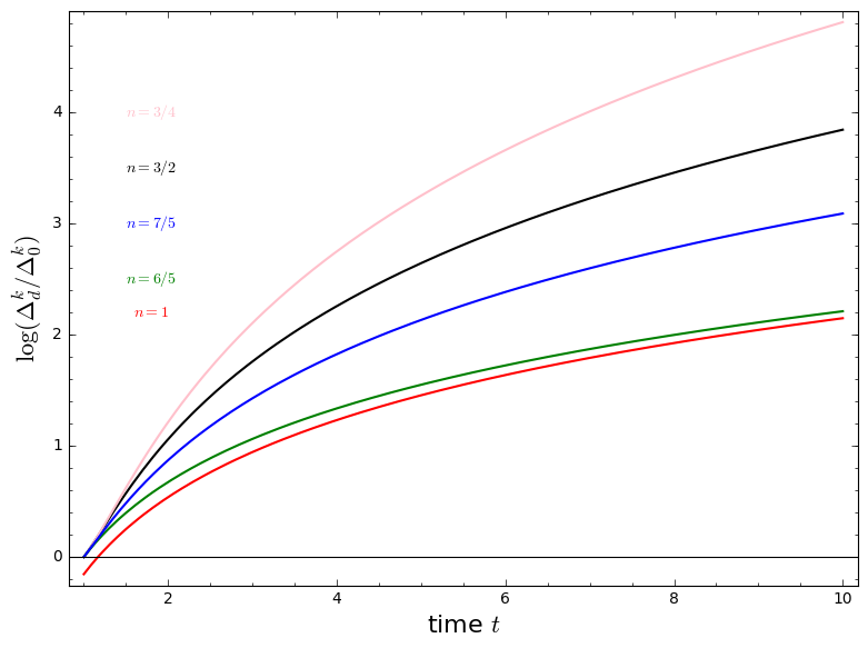
Figure 1: Solution to Eq. (76) for different values of $n$ with assumption that $\Delta^{k}_{(d)0}=10^{-3},\dot{\Delta}^{k}_{(d)0}=10^{-3}$

9.2 Scalar field-radiation system

For a universe composed of a mixture of the scalar field together with the radiation matter content, we can still assume that the background is filled with a scalar field in a flat FLRW spacetime. Since for radiation $w_{r}=\frac{1}{3}$, we have the perturbation equations as

$$\dot{\Delta}^{k}_{r}=-\frac{4}{3}Z^{k}+\frac{\Theta}{3}\Delta^{k}_{r}\;,$$ (83)

$$\begin{split}\dot{Z}^{k}&=\Big{(}\frac{\dot{\phi}}{\phi+1}-\frac{2\Theta}{3}\Big{)}Z^{k}+\Big{[}\frac{(\phi-3)}{4(\phi+1)}\mu_{r}-\frac{1}{4}\Big{(}-\frac{1}{3}\Theta^{2}+\frac{f}{2(\phi+1)}\\ &+\frac{\Theta\dot{\phi}}{\phi+1}+\frac{k^{2}\phi^{\prime}R}{a^{2}(\phi+1)}\Big{)}+\frac{k^{2}}{4a^{2}}\Big{]}\Delta^{k}_{r}+\frac{\Theta}{\phi+1}\Psi^{k}\;,\end{split}$$ (84)

$$\begin{split}\dot{\Psi}^{k}&=-\frac{\ddot{\phi}}{4}\Delta^{k}_{r}\;.\end{split}$$ (85)

We therefore have equation in $\Delta^{k}_{r}$ as

$$\begin{split}&\ddot{\Delta}^{k}_{r}-\Big{(}\frac{\dot{\phi}}{\phi+1}-\frac{\Theta}{3}\Big{)}\dot{\Delta}^{k}_{r}-\Big{[}\frac{2\Theta}{9}-\frac{\dot{\phi}}{3(\phi+1)}-\frac{(\phi-3)\mu_{r}}{3(\phi+1)}-\frac{1}{9}\Theta^{2}+\frac{f}{6(\phi+1)}\\ &+\frac{7\Theta\dot{\phi}}{12(\phi+1)}+\frac{k^{2}\phi^{\prime}R}{3a^{2}(\phi+1)}+\frac{\dot{\Theta}}{3}-\frac{k^{2}}{3a^{2}}\Big{]}\Delta^{k}_{r}=0\;.\end{split}$$ (86)

At this stage, if we consider $R^{n}$ models, where we can take the exact single fluid background transient solution as

$$a=t^{\frac{n}{2}}\;.$$ (87)

In this context, Eqs (65)- (67) reduce to

$$\Theta=\frac{3n}{2t}\;,$$ (88)

$$R=\frac{3n(n-1)}{t^{2}}\;,$$ (89)

$$\mu_{r}=\Big{(}\frac{3}{4}\Big{)}^{2-n}\Big{(}\frac{9n(n-1)}{4t^{2}}\Big{)}^{n-1}\Big{(}\frac{-5n^{3}+8n^{2}-2n}{t^{2}}\Big{)}\;,$$ (90)

and scalar field has the form

$$\phi=n\left(\frac{3n(n-1)}{t^{2}}\right)^{n-1}-1\;.$$ (91)

We can write Eq. (86) as

$$\begin{split}&\ddot{\Delta}^{k}_{r}+A_{1}(t)\dot{\Delta}^{k}_{r}+A_{2}(t)\Delta^{k}_{r}=0\;,\end{split}$$ (92)

where

$$A_{1}(t)=\frac{(-5n+4)}{2t}\;,$$ (93)

and

$$\begin{split}&A_{2}(t)=-\frac{(-3n^{2}+3n-2)}{3t}-\frac{(-11n^{2}+3n-4)}{4t^{2}}-\frac{k^{2}(n-2)}{3t^{n}}\\ &+\frac{3^{1-n}}{16t^{2}}\Big{[}n\Big{(}\frac{4n(4n-4)}{16/3}\Big{)}^{n-1}t^{-2(n-1)}-2\Big{]}(-20n^{3}+32n^{2}-8n)\;.\end{split}$$ (94)

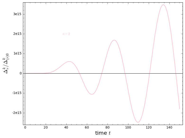
Figure 2: Solution of fractional radiation energy density fluctuations for $n=2$, with assumption that $\Delta^{k}_{(d)0}=10^{-4},\dot{\Delta}^{k}_{(d)0}=10^{-4}$

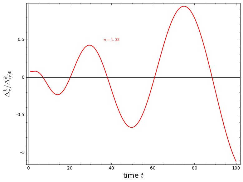
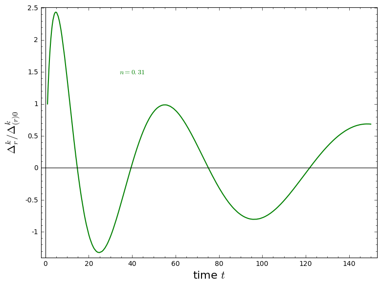
Figure 3: Solution of fractional radiation energy density fluctuations for $n=1.23$, with assumption that $\Delta^{k}_{(d)0}=10^{-4},\dot{\Delta}^{k}_{(d)0}=10^{-4}$

Figure 4: Solution of fractional radiation energy density fluctuations for $n=0.31$, with assumption that $\Delta^{k}_{(d)0}=10^{-4},\dot{\Delta}^{k}_{(d)0}=10^{-4}$

The numerical solutions of Eq. (92) are obtained for $n=2$, $n=1.23$ and $n=0.31$ and plotted in Fig.2, Fig. 4 and Fig. 4 respectively. During the numerical computation, the assumption of long wavelength is made for simplicity; that is, we have assumed that $k^{2}$ is small enough compared to other terms (or $\frac{k^{2}}{a^{2}H^{2}}<<1$). However, the behavior of this solution is oscillatory with changing in amplitude. Since we are dealing with the system where the scalar field was dominating in flat FLRW spacetime, the treatment was that the radiation energy perturbations are the ones expected to rise. Thus, surprisingly, it turns out that these perturbations grow in an oscillatory shape. The oscillatory solution of this type has been obtained for GR case in Ref. [30]. This behavior is also observed in Fig. 4. We therefore say that for $n>1$, we have oscillator grow in amplitude radiation fluctuations. But if one looks at the case of $n=0.31$, that is $0<n<1$, (see Fig. 4 ) we realized that the perturbations have high amplitude and later decays in oscillatory way. Therefore, we can say that the weaker gravity $(n<1)$, tend not to have growing radiation perturbations, yet the high gravity, that is $n>1$, clearly has a hand on the growth of the radiation perturbations.

10 Conclusions and discussions

In this paper we have studied linear cosmological perturbations of a flat FLRW spacetime background using the $1+3$ covariant and gauge-invariant formalism, where the Brans-Dicke scalar-tensor theory is the underlying model of gravitation assumed. We have used the equivalence between the scalar-tensor and $f(R)$ gravity theories to develop perturbation equations based on gradient variables defined in a covariant and gauge-invariant way. The extra degree of freedom that differentiates $f(R)$ from GR is defined to be an extra scalar-field degree of freedom. Thus the density perturbations considered correspond to a scalar field–standard matter two-fluid cosmic medium. We have then specialized to a scalar field-dust and scalar field-radiation fluid systems to analyse some interesting solutions. The energy density perturbations of dust grow exponentially in time for different values of $n$. This result is in agreement with the existing literature about perturbations of $R^{n}$ gravity toy models. For the case of the radiation-dominated epoch, the behavior of the amplitude of the radiation perturbations depends on the nature of $n$. For $n$ less than unity, the perturbations decay with time in oscillatory mode, but for the values of $n$ greater than unity, the fluctuations grow and oscillate. This radiation perturbations behavior is studied under long-wavelength assumption. A more detailed analysis is needed in the context of non-vanishing scalar field perturbations.

Appendix

In this Appendix, we present the relationship between curvature gradient $\mathcal{R}_{a}$ and $\Phi_{a}$ as

$$\mathcal{R}_{a}=\frac{\Phi_{a}}{\phi^{\prime}}\;.$$ (95)

The relationship between curvature momentum gradient $\Re_{a}$ and, $\Phi_{a}$ and scalar field momentum gradient $\Psi_{a}$ is given

$$\Re_{a}=\frac{\Psi_{a}}{\phi^{\prime}}-\frac{\dot{\phi}\phi^{\prime\prime}}{\phi^{\prime 3}}\Phi_{a}\;,$$ (96)

where $\mathcal{R}_{a}=a\tilde{\nabla}_{a}R$ and $\Re_{a}=a\tilde{\nabla}_{a}\dot{R}$. We provide equations relating covariant quantities between both theories: $f(R)$ and Scalar tensor theories. We start by obtaining the scalar variables from equations (95) and (96) as

$$\mathcal{R}=\frac{\Phi}{\phi^{\prime}}\;,$$ (97)

$$\Re=\frac{\Psi}{\phi^{\prime}}-\frac{\dot{\phi}\phi^{\prime\prime}}{\phi^{\prime 3}}\Phi\;,$$ (98)

where $\mathcal{R}=a\tilde{\nabla}^{a}\mathcal{R}_{a}$ and $\Re=a\tilde{\nabla}^{a}\Re_{a}$. Thus one has the evolution equations of perturbation quantities as

$$\dot{\Delta}_{m}=-(1+w)Z+w\Theta\Delta_{m}\;,$$ (99)

$$\begin{split}\dot{Z}&=\Big{(}\frac{\dot{\phi}}{\phi+1}-\frac{2\Theta}{3}\Big{)}Z-\frac{w}{(1+w)}\tilde{\nabla}^{2}\Delta_{m}-\frac{\phi^{\prime}}{\phi+1}\tilde{\nabla}^{2}\mathcal{R}+\Big{[}\frac{1}{2\phi^{\prime}}+\frac{\mu_{m}}{(\phi+1)^{2}}-\frac{f}{2(\phi+1)^{2}}\\ &-\frac{\Theta\dot{\phi}}{(\phi+1)^{2}}-\frac{\phi^{\prime\prime}\tilde{\nabla}^{2}R}{\phi^{\prime}(\phi+1)}+\frac{\phi^{\prime}\tilde{\nabla}^{2}R}{(\phi+1)^{2}}-\frac{2K}{(\phi+1)a^{2}}+\frac{\Theta\dot{\phi}\phi^{\prime\prime}}{\phi^{\prime 2}(\phi+1)}\Big{]}\phi^{\prime}\mathcal{R}+\frac{\Theta\phi^{\prime}}{\phi+1}\Re\\ &+\Big{[}\frac{\phi w-1}{(w+1)(\phi+1)}\mu_{m}-\frac{w}{1+w}\Big{(}-\frac{1}{3}\Theta^{2}+\frac{f}{2(\phi+1)}+\frac{\Theta\dot{\phi}}{\phi+1}-\frac{\phi^{\prime}}{\phi+1}\tilde{\nabla}^{2}R\Big{)}\Big{]}\Delta_{m}\;,\end{split}$$ (100)

$$\dot{\mathcal{R}}=-\Big{(}\frac{\dot{\phi}^{\prime}}{\phi^{\prime}}-\frac{\dot{\phi}\phi^{\prime\prime}}{\phi^{\prime}}\Big{)}\mathcal{R}+\phi^{\prime}\Re-\frac{w\dot{\phi}}{w+1}\Delta_{m}\;,$$ (101)

$$\begin{split}\dot{\Re}&=-\Big{\{}\frac{\dot{\phi}^{\prime}}{\phi^{\prime}}+\frac{\dot{\phi}\phi^{\prime\prime}}{\phi^{\prime}}-\frac{\dot{\phi}\phi^{\prime\prime}}{\phi^{\prime}}\Big{(}\dot{\phi}^{\prime}+\frac{\dot{\phi}^{\prime}}{\phi^{\prime}}-2\Big{)}-\frac{\dot{\phi}^{\prime}}{\phi^{\prime}}\Big{\}}\Re-\Big{\{}\frac{\ddot{\phi}\phi^{\prime\prime}}{\phi^{\prime 2}}+\frac{\dot{\phi}\dot{\phi}^{\prime\prime}}{\phi^{\prime 2}}-\frac{\dot{\phi}\dot{\phi}^{\prime}\phi^{\prime\prime}}{\phi^{\prime 3}}-\frac{\dot{\phi}\phi^{\prime\prime}}{\phi^{\prime 2}}\Big{(}\frac{\dot{\phi}^{\prime}}{\phi^{\prime}}\\ &-\frac{\dot{\phi}\phi^{\prime\prime}}{\phi^{\prime}}\Big{)}-\Big{[}\frac{\dot{\phi}\phi^{\prime\prime}}{\phi^{\prime}}\Big{(}\dot{\phi}^{\prime}+\frac{\dot{\phi}^{\prime}}{\phi^{\prime}}-2\Big{)}+\frac{\dot{\phi}^{\prime}}{\phi^{\prime}}\Big{]}\frac{\dot{\phi}\phi^{\prime\prime}}{\phi^{\prime}}+\frac{\phi^{\prime\prime}}{\phi^{\prime}}\Big{[}\frac{\dot{\phi}^{2}}{\phi^{\prime}}\Big{(}1+\frac{1}{\phi^{\prime}}\Big{)}(\frac{\phi^{\prime\prime\prime}}{\phi^{\prime\prime}}-\frac{\phi^{\prime\prime}}{\phi^{\prime}})-\frac{\dot{\phi}^{2}}{\phi^{\prime}}\frac{\phi^{\prime\prime\prime}}{\phi^{\prime\prime}}\\ &+\frac{\dot{\phi}^{2}\phi^{\prime\prime}}{\phi^{\prime 2}}-\frac{\dot{\phi}\dot{\phi}^{\prime}}{\phi^{\prime 2}}\Big{]}\Big{\}}\mathcal{R}+\Big{(}\frac{w\dot{\phi}^{2}\phi^{\prime\prime}}{\phi^{\prime 2}(w+1)}-\frac{w\ddot{\phi}}{\phi^{\prime}(w+1)}\Big{)}\Delta_{m}\;,\end{split}$$ (102)

and constraint equation is given as

$$\begin{split}\frac{C}{a^{2}}&=-\Big{(}\frac{4}{3}\Theta+\frac{2\ddot{\phi}}{\phi+1}\Big{)}Z+\frac{2\mu_{m}}{\phi+1}\Delta_{m}+\frac{2\phi^{\prime}}{\phi+1}\tilde{\nabla}^{2}\mathcal{R}+\Big{\{}\Big{[}-\frac{2\mu_{m}}{(\phi+1)^{2}}+\frac{f}{(\phi+1)^{2}}\\ &-\frac{2\Theta}{\phi+1}\frac{\phi^{\prime\prime}}{\phi^{\prime}}\Big{(}\frac{\dot{\phi}^{2}}{\phi^{\prime}}(\frac{\phi^{\prime}+1}{\phi^{\prime}})(\frac{\phi^{\prime\prime\prime}}{\phi^{\prime\prime}}-\frac{\phi^{\prime\prime}}{\phi^{\prime}})-\frac{\dot{\phi}^{2}}{\phi^{\prime}}\frac{\phi^{\prime\prime\prime}}{\phi^{\prime\prime}}\frac{\dot{\phi}^{2}\phi^{\prime\prime}}{\phi^{\prime 2}}-\frac{\dot{\phi}\dot{\phi}^{\prime}}{\phi^{\prime 2}}\Big{)}+\frac{2\Theta\ddot{\phi}}{\phi+1}+\frac{4K}{a^{2}(\phi+1)}\\ &+\frac{2\phi^{\prime\prime}\tilde{\nabla}^{2}R}{(\phi+1)\phi^{\prime}}-\frac{2\phi^{\prime}\tilde{\nabla}^{2}R}{(\phi+1)^{2}}\Big{]}\phi^{\prime}-\frac{2\Theta}{\phi+1}\Big{[}\Big{(}\dot{\phi}+\frac{\dot{\phi}}{\phi^{\prime}}\Big{)}\frac{\phi^{\prime\prime}}{\phi^{\prime}}+\dot{\phi}^{\prime}-\frac{2\dot{\phi}\phi^{\prime\prime}}{\phi^{\prime}}+\frac{\dot{\phi}^{\prime}}{\phi^{\prime}}\Big{]}\frac{\dot{\phi}\phi^{\prime\prime}}{\phi^{\prime}}\Big{\}}\mathcal{R}\\ &-\frac{2\Theta}{\phi+1}\Big{[}\Big{(}\dot{\phi}+\frac{\dot{\phi}}{\phi^{\prime}}\Big{)}\frac{\phi^{\prime\prime}}{\phi^{\prime}}+\dot{\phi}^{\prime}-\frac{2\dot{\phi}\phi^{\prime\prime}}{\phi^{\prime}}+\frac{\dot{\phi}^{\prime}}{\phi^{\prime}}\Big{]}\phi^{\prime}\Re\;.\end{split}$$ (103)

References

- [1] T Singh and Tarkeshwar Singh. General class of scalar-tensor theories: A review. International Journal of Modern Physics A, 2(03):645–666, 1987.
- [2] Yasunori Fujii and Kei-ichi Maeda. The scalar-tensor theory of gravitation. Cambridge University Press, 2003.
- [3] Carl H Brans. Scalar-tensor theories of gravity: Some personal history. In AIP Conference Proceedings, volume 1083, pages 34–46. AIP, 2008.
- [4] Yasunori Fujii. Some aspects of the scalar-tensor theory. arXiv preprint gr-qc/0410097.
- [5] Thomas P Sotiriou and Valerio Faraoni. theories of gravity. Reviews of Modern Physics, 82(1):451, 2010.
- [6] Timothy Clifton, Pedro G Ferreira, Antonio Padilla, and Constantinos Skordis. Modified gravity and cosmology. Physics Reports, 513(1):1–189, 2012.
- [7] Sumanta Chakraborty and Soumitra SenGupta. Solving higher curvature gravity theories. The European Physical Journal C, 76(10):552, 2016.
- [8] Andrei V Frolov. Singularity problem with models for dark energy. Physical review letters, 101(6):061103, 2008.
- [9] Baojiu Li and John D Barrow. Cosmology of gravity in the metric variational approach. Physical Review D, 75(8):084010, 2007.
- [10] Valerio Faraoni. de sitter space and the equivalence between and scalar-tensor gravity. Physical Review D, 75(6):067302, 2007.
- [11] Joseph Ntahompagaze, Amare Abebe, and Manasse Mbonye. On gravity in scalar–tensor theories. International Journal of Geometric Methods in Modern Physics 14.7, page 1750107, 2017.
- [12] Heba Sami, Neo Namane, Joseph Ntahompagaze, Maye Elmardi, and Amare Abebe. Reconstructing gravity from a chaplygin scalar field in de sitter spacetimes. International Journal of Geometric Methods in Modern Physics 15: 1850027., 2017.
- [13] Heba Sami, Joseph Ntahompagaze, and Amare Abebe. Inflationary cosmologies. Universe 3.4: 73, 2017.
- [14] R Treciokas and GFR Ellis. Isotropic solutions of the einstein-boltzmann equations. Communications in Mathematical Physics, 23(1):1–22, 1971.
- [15] George FR Ellis and Marco Bruni. Covariant and gauge-invariant approach to cosmological density fluctuations. Physical Review D, 40(6):1804, 1989.
- [16] Marco Bruni, Peter KS Dunsby, and George FR Ellis. Cosmological perturbations and the physical meaning of gauge-invariant variables. The Astrophysical Journal, 395:34–53, 1992.
- [17] Amare Abebe. Breaking the cosmological background degeneracy by two-fluid perturbations in gravity. International Journal of Modern Physics D, 24(07):1550053, 2015.
- [18] Kishore N Ananda, Sante Carloni, and Peter KS Dunsby. A detailed analysis of structure growth in theories of gravity. arXiv preprint arXiv:0809.3673, 2008.
- [19] Sante Carloni, Peter KS Dunsby, and Claudio Rubano. Gauge invariant perturbations of scalar-tensor cosmologies: The vacuum case. Physical Review D, 74(12):123513, 2006.
- [20] Bob Osano, Cyril Pitrou, Peter Dunsby, Jean-Philippe Uzan, and Chris Clarkson. Gravitational waves generated by second order effects during inflation. Journal of Cosmology and Astroparticle Physics, 2007(04):003, 2007.
- [21] Amare Abebe, Mohamed Abdelwahab, Alvaro de la Cruz-Dombriz, and Peter KS Dunsby. Covariant gauge-invariant perturbations in multifluid gravity. Classical and quantum gravity, 29(13):135011, 2012.
- [22] Sumanta Chakraborty and Soumitra SenGupta. Gravity stabilizes itself. arXiv preprint arXiv:1701.01032, 2016.
- [23] Sante Carloni, Emilio Elizalde, and Sergei Odintsov. Conformal transformations in cosmology of modified gravity: the covariant approach perspective. General Relativity and Gravitation, 42(7):1667–1705, 2010.
- [24] Thomas Faulkner, Max Tegmark, Emory F Bunn, and Yi Mao. Constraining gravity as a scalar-tensor theory. Physical Review D, 76(6):063505, 2007.
- [25] John M Stewart and Martin Walker. Perturbations of space-times in general relativity. In Proceedings of the Royal Society of London A: Mathematical, Physical and Engineering Sciences, volume 341, pages 49–74. The Royal Society, 1974.
- [26] Sante Carloni. Covariant gauge invariant theory of scalar perturbations in -gravity: A brief review. Open Astronomy Journal, 3:76–93, 2010.
- [27] Marco Bruni, George FR Ellis, and Peter KS Dunsby. Gauge-invariant perturbations in a scalar field dominated universe. Classical and Quantum Gravity, 9(4):921, 1992.
- [28] GFR Ellis, M Bruni, and J Hwang. Density-gradient-vorticity relation in perfect-fluid robertson-walker perturbations. Physical Review D, 42(4):1035, 1990.
- [29] Sante Carloni, Peter KS Dunsby, Salvatore Capozziello, and Antonio Troisi. Cosmological dynamics of gravity. Classical and Quantum Gravity, 22(22):4839, 2005.
- [30] George FR Ellis, Roy Maartens, and Malcolm AH MacCallum. Relativistic cosmology. Cambridge University Press, 2012.