Self-excitation in a helical liquid metal flow: The Riga dynamo experiments

Abstract

The homogeneous dynamo effect is at the root of magnetic field generation in cosmic bodies, including planets, stars and galaxies. While the underlying theory had increasingly flourished since the middle of the 20th century, hydromagnetic dynamos were not realized in laboratory until 1999. On 11 November 1999, this situation changed with the first observation of a kinematic dynamo in the Riga experiment. Since that time, a series of experimental campaigns has provided a wealth of data on the kinematic and the saturated regime. This paper is intended to give a comprehensive survey about these experiments, to summarize their main results and to compare them with numerical simulations.

1 Introduction

The seminal paper of Steenbeck, Krause & Rädler (1966), which is celebrated in this special issue, was not only a landmark in the theoretical description of cosmic dynamos, but had also fostered a series of experimental activities. One of them was the experimental demonstration of the $\alpha$–effect in the Riga “$\alpha$–box,” a system of two orthogonally interlaced copper channels (Steenbeck et al. 1967). Since the sodium flow through this system was not mirror-symmetric, it produced a measurable $\alpha$–effect, as confirmed by the observations that the induced voltage in weak fields was proportional to $Bv^{2}$ while it changed sign when the applied magnetic field was reversed.

In the same year, the first author of this paper (Gailitis 1967) proposed an experimental dynamo “in which the gyrotropic turbulence is simulated by means of a certain pseudo-turbulent motion.” This early idea to substitute real helical (“gyrotropic”) turbulence by “pseudo-turbulence” was later to be realized in the two-scale Karlsruhe dynamo experiment by using 52 parallel channels with helical sodium flows inside (Müller & Stieglitz 2000; Stieglitz & Müller 2001; Müller, Stieglitz & Horanyi 2004; Müller, Stieglitz & Horanyi 2004).

Meanwhile, the focus in Riga had shifted away from the two-scale, multi-channel flow dynamo towards a dynamo concept based on a single helical flow. This development was ignited by the paper of Ponomarenko (1973) who had proved dynamo action for a solid conducting rod screwing through a medium of infinite extend with which it is in sliding electrical contact.

In a detailed numerical analysis of this ”elementary cell” of a dynamo, Gailitis and Freibergs (1976) had computed a remarkable low critical magnetic Reynolds number of 17.7 for the convective instability. Later it was found that by adding a concentric straight backflow to the helical flow this convective instability could be rendered an absolute one (Gailitis and Freibergs 1980).

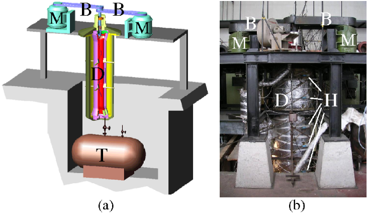
Figure 1: Sketch (a) and photograph (b) of the Riga dynamo facility, with the central dynamo module (D) mounted on a steel frame, the two DC-motors (M), the belts (B), one of the storage tanks (T), and the external Hall sensors (H).

The Riga dynamo experiment (figure 1) is the laboratory realization of this principle of magnetic field self-excitation in a single helical flow. At this facility, an exponentially growing eigenmode was observed for the first time in November 1999 (Gailitis et al. 2000a). A follow-up experiment, reaching also the saturation regime, was carried out in July 2000 and reported in a number of papers (Gailitis et al. 2001a; Gailitis et al. 2001b).

Since those days, a number of further experimental campaigns have been carried out: the experiments in June 2002, February 2003, July 2003, May 2004, February/March 2005, and July 2007 have brought about many details on the spatial and temporal magnetic field structure, due to a step-by-step improvement of the measuring system. The wealth of new data has led to an improved understanding of the experiment, which we would like to report on in this survey. Their correspondence with numerical simulations will be another focus of this paper.

After three further campaigns in April 2009 and February and June 2010, which were less successful due to several technical problems, the Riga dynamo was disassembled and completely reconstructed, before two new campaigns were carried out in June 2016 and April 2017. Their results, however, will be discussed elsewhere.

2 Theory and numerics

Dynamo theory is governed by two coupled equations. The first one is the induction equation for the magnetic field $\bf B$,

$$\frac{\partial{{\bf{B}}}}{\partial t}=\nabla\times({\bf{v}}\times{\bf{B}})+\frac{1}{\mu_{0}\sigma}\Delta{\bf{B}}\;,$$ (1)

where $\bf v$ denotes the velocity field of the fluid, $\sigma$ its electrical conductivity and $\mu_{0}$ the magnetic permeability of the free space. Equation (1) follows directly from Ampère’s, Faraday’s and Ohm’s law. In its derivation, quasi-stationarity is assumed in the sense that the displacement current can be neglected.

Evidently, without any flow velocity, (1) reduces to a diffusion equation which describes the free decay of the magnetic field in an electrically conducting medium. The velocity dependent term can, under certain conditions for the strength and topology of the flow, counteract this decay and lead to a positive gain for the magnetic field.

As long as the velocity is stationary, (1) can be transformed into an eigenvalue equation

$$\lambda{\bf{B}}=\nabla\times({\bf{v}}\times{\bf{B}})+\frac{1}{\mu_{0}\sigma}\Delta{\bf{B}}\;,$$ (2)

with $\lambda=p+2\pi if$, including the growth rate $p$ and the frequency $f$. It is rather typical for dynamos that they are governed by non-self-adjoint induction operators, which may have, in general, complex eigenvalues.

In case of a positive growth rate, the magnetic field will increase exponentially until it reaches such an amplitude that the back-reaction of the Lorentz forces on the velocity is not negligible anymore. Then it becomes necessary to consider also the Navier-Stokes equation

$$\frac{\partial{{\bf{v}}}}{\partial t}+({\bf{v}}\cdot\nabla){\bf{v}} = -\frac{\nabla p}{\rho}+\frac{1}{\mu_{0}\rho}(\nabla\times{\bf{B}})\times{\bf{B}}+\nu\Delta{\bf{v}}+{\bf{f}}_{prop}\;,$$ (3)

where $\rho$ and $\nu$ denote the density and the kinematic viscosity of the fluid, and ${\bf{f}}_{prop}$ symbolizes the force exerted by the propeller (in our context). Typically, the dynamo will saturate into a state where the Lorentz forces act against the source of its generation (Lenz’s rule).

2.1 Kinematic regime of the Riga dynamo

The basic idea of the Riga dynamo experiment traces back to the paper of Ponomarenko (1973) who had proved that dynamo action can occur when a conducting rod of infinite length screws slidingly through a conducting medium of infinite radial extension.

In a more detailed numerical analysis of this ”elementary cell” of a dynamo, Gailitis and Freibergs (1976) had found a remarkable low critical magnetic Reynolds number of 17.7 for the convective instability. By adding a back-flow, this convective instability can be made into an absolute instability (Gailitis & Freibergs 1980). All these early computations, including the main geometric optimization of the three cylinders configuration (Gailitis 1996), were carried out with a one-dimensional code in which the induction equation (1) was reduced to three coupled radial equations for the components of $\tilde{\bf B}(r,\lambda)$, defined via ${\bf{B}}(r,\phi,z,t)=\exp{(im\phi+ikz+\lambda t)}\tilde{\bf B}(r,\lambda)$. Such a simplification is well justified in case that the velocity is independent of $\phi$, $z$ and $t$. The method is not restricted to study convective instabilities; using spatially growing modes it can also be employed to identify absolute instabilities by searching for saddle-points in the complex plane which indicate zero group velocity.

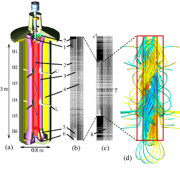
Figure 2: (a) Central module of the Riga dynamo experiment, (b,c) geometrical simplification for 2D numerical simulations, and (d) the structure of its eigenfield. 1 - Propeller region; 2 - Helical flow region; 3 - Back-flow region; 4 - Outer sodium filled cylinder; 5 - Straightening region behind the lower bending; 6 - Lower bending; 7 - Upper bending; U - Upper port; L - Lower Port; H1…H6 - External Hall sensors. (c) Embedding of the dynamo in vacuum. The grid number is 401 in axial direction and 64 in radial direction. Note the non-uniform grid spacing with the finest resolution in the bending regions. The snapshot of the computed magnetic field lines in the kinematic regime was computed for a propeller rotation rate of 2000 rpm. The field pattern rotates with a frequency of 1.16 Hz around the vertical axis, in the same direction as the flow. The color of the field-lines indicates the z-component of the field. The red frame indicates the simplified geometry as it is used in the simulations.

Complementary to this 1D code, a two-dimensional (2D) code was developed which, as long as the velocity is unchanged along the vertical axis, provided results very close to those of the 1D code (Stefani, Gailitis & Gerbeth 1999; Gailitis et al. 2004). Its main advantage is the possibility to cope also with velocity fields varying along the axis of the dynamo. This 2D code, which was used for many simulations of the Riga dynamo, is a finite difference scheme on a non-homogeneous grid, with an Adams-Bashforth method of second order for the time integration. The real geometry of the dynamo module has been slightly simplified (see figure 2b,c), with all curved parts in the bending regions being replaced by rectangles. The velocity in the central cylinder was inferred from a number of measurements at a water test facility and some extrapolations (Christen, Hänel & Will 1998; Stefani, Gailitis & Gerbeth 1999). These measurements had revealed a slight decay of the rotational component along the flow. The axial velocity in the back-flow region was assumed as purely axial and constant so that the mean flow is equivalent to that in the inner cylinder. In the bending regions some simplified flow structures were employed, ensuring the divergence-free condition and rather smooth transitions from the central to the back-flow cylinder and vice-versa. In the propeller region the rotational component is assumed to increase linearly.

Appropriate interface condition were applied at the walls of the cylinders where velocity jumps occur. The three conditions used in the numerical scheme are that the two tangential components of the electric field are continuous and that the divergence is zero. A notorious problem for dynamos in non-spherical geometry is the treatment of the boundary conditions at the outer rim (Stefani, Giesecke & Gerbeth 2009). Our solution for this problem was as follows: in the dynamo domain, the Adams-Bashforth-scheme was applied. For every time-step, we solved the Laplace equation for the magnetic field in the exterior of the domain by means of a pseudo-transient relaxation. At the outer boundary of this extended domain we use zero boundary conditions, whereas at the interface to the dynamo we use the interface conditions. Admittedly this is a tedious and time-consuming procedure. However, since a simpler method of using vertical field conditions lead to a remarkable underestimation of the critical magnetic Reynolds number, the correct treatment of the exterior pays off when it comes to an accurate prediction of the dynamo.

Figure 2d gives an impression of the magnetic field line structure as it results from the 2D code. The double-helix field structure is clearly visible. Note that this is a snapshot of the field pattern which actually corotates with the flow around the vertical direction, although with a much lower frequency than the rotational velocity.

2.2 Saturation regime of the Riga dynamo

In contrast to the kinematic regime, the understanding of the saturation regime is much more intriguing. In principle, it requires the fully coupled three-dimensional numerical simulation of the induction and Navier-Stokes equations, the latter one at a Reynolds number of appr. $2\times 10^{6}$. While related numerical efforts have indeed been undertaken by using a RANS turbulence model (Kenjereš et al. 2006; Kenjereš & Hanjalić 2006; Kenjereš & Hanjalić 2007), we will rely in the following on the simple back-reaction mechanism as described by Gailitis et al. (2002b).

In this model we focus on the dominant effect of braking the azimuthal component. We start by splitting the velocity field into an undisturbed part ${\bar{\bf{v}}}$, which we assume to be a solution of equation (3) without the Lorentz force term, and a perturbation ${\delta{\bf{v}}}$ which we assume to be caused by the Lorentz force. The same splitting is done for the pressure: $p=\bar{p}+\delta p$.

In the first order approximation we can now compute the magnetic field ${\bf{B}}$ for a given (i.e., measured or interpolated) undisturbed $\bar{\bf{v}}$ using the induction equation, and insert the resulting magnetic field into the linearized Navier-Stokes equation for the flow perturbation ${\delta{\bf{v}}}$,

$$\frac{\partial{{\delta{\bf{v}}}}}{\partial t}+({\bar{\bf{v}}}\cdot\nabla){{\delta{\bf{v}}}}+({\delta{\bf{v}}}\cdot\nabla){{\bar{\bf{v}}}}= \frac{1}{\mu_{0}\rho}(\nabla\times{\bf{B}})\times{\bf{B}}-\frac{\nabla\delta p}{\rho}+\nu\Delta{\delta{\bf{v}}}\;.$$ (4)

In principle, this perturbation method can be extended to higher orders by inserting the resulting $\bf{v}={\bar{\bf{v}}}+{\delta{\bf{v}}}$ again into the induction equation, and so on.

Here, we present a simplified version which will later be shown to explain the observed back-reaction effects. The simplifications are as follows: First, we restrict the perturbation method to the first order. Second we skip the viscous term in equation (4). Third, we restrict all back-reaction effects to their axisymmetric contribution (since the azimuthal dependence of the self-excited magnetic field is proportional to $\exp{(im\phi)}$ with $m=1$, the Lorentz force in Equation (4) contains terms with $m=0$ and $m=2$ leading to corresponding velocity and pressure perturbations). Fourth, we do not even solve the simplified equation (4) but concentrate on the azimuthal component. This simplification is motivated by the fact that one can expect the $z$-component of the Lorentz force to result in an additional pressure gradient in $z$-direction and not into a velocity decrease (the total flowrate $\int rv_{z}drd\phi$ has to be constant along the $z$-axis). The remaining rotational part of the radial and the axial force will, of course, result in some deformation of the velocity profile. The only component of the $m=0$ Lorentz force part which by no means can be absorbed into a pressure gradient is the azimuthal one on which we focus in the following.

After all, we solve the ordinary differential equation for the perturbation $\delta v_{\phi}$,

$$\bar{v}_{z}\frac{\partial}{\partial z}\delta v_{\phi}=\frac{1}{\mu_{0}\rho}[(\nabla\times{\bf{B}})\times{\bf{B}}]_{\phi}\;,$$ (5)

both in the helical flow region and in the back-flow region. As shown in Gailitis et al. (2002b), the Lorentz force resulting from the magnetic eigenfield illustrates Lenz’s rule. Its axial component breaks the axial velocity in both flow regions, thereby leading to a pressure increase which has to be overcome by additional power of the motors. At the same time, the azimuthal component leads to reduction of the differential rotation, by reducing the rotation in the helical flow region and accelerating it in the back-flow region. This way, the generation capacity of the saturated dynamo decreases along the downward flow, which finally leads to a general upward shift of the eigenfield.

3 The facility and the experimental campaigns

After, in 1987, a forerunner experiment had shown significant field amplification but no self-excitation (Gailitis et al. (1987), more than a decade was spent on the design and the optimization of the present machine. The overall structure is depicted in figure 1: the central module of approximately 3 m length and 0.8 m diameter is mounted on a steel frame. The power for the propeller is provided by two DC-motors, which can be driven up to 200 kW. Before and after the experimental campaigns the sodium resides in two storage tanks.

Basically, the dynamo module consists of three concentric cylinders with different flow structures (figure 2a). In the central cylinder the sodium is forced by the propeller, and guided by pre- and post-propeller vanes, on a helical path with an appropriate relation of axial and azimuthal velocity components and an optimized radial dependence of both. After the flow swirl is taken out by some blades in the lower bending region, the flow becomes basically rotation-free in the back-flow cylinder, although the back-reaction of the magnetic field in the saturation regime will induce some rotation within this tube. The same holds for the third, outermost, cylinder where the sodium is stagnant at the beginning of the experiment, but where the Lorentz forces will also drive some flow when the magnetic field has become strong enough.

In the following we will summarize the results of the experimental campaigns carried out between 1999 and 2007.

3.1 November 1999

The main result of the experimental campaign in November 1999 was the detection of a flow induced, slowly growing eigenmode of the dynamo. Since in this first experiment the main focus laid on the study of the amplification of an externally applied field, the detection of the self-excited mode was more a less a by-product.

Figure 3a shows the magnetic field as measured by one of the external Hall sensors (H4, situated at a vertical distance of 1.85 m from upper frame) over a time span of 400 seconds. During this time, the propeller rotation rate went up from 1000 rpm to 2150 rpm, then it remained for a while at 1980 rpm before being reduced to zero. During this time the signal of the external Hall sensor changes only slightly, with a shallow maximum at approx. 1800 rpm. What the Hall sensor sees here is essentially the magnetic field from the external excitation coils which is only slightly modified by the induction effect of the sodium flow. The maximum at 1800 rpm can be understood when showing (see figure 3b) the ratio of external coil current to the magnetic field as measured by an internal fluxgate sensor. This ratio is a measure of the inverse amplification of the externally applied excitation field. Irrespective of some particular dependencies on the frequency and the phase relation of the external 3-phase current, this ratio shows a clear minimum at around 1800 rpm, with the amplification reaching a value of 20. However impressive this factor might appear, it testifies only a strong amplification, but not self-excitation! All the data points shown in figure 3b rely on measured magnetic field data with exactly the frequency of the external excitation.

The only exception is the rightmost point. Here, at a rotation rate of 2150 rpm (and a still rather high temperature of 210^∘C), a superposition of the amplified excitation signal (at 1 Hz) and a self-excited eigenmode (1.326 Hz) was recorded for a period of 15 seconds (the interval between 350 s and 365 s in figure 3c). Yet, this period was too short to allow the field to grow to values relevant for back-reaction effects. Soon after that measurement, the rotation rate was reduced to 1980 rpm, where the excitation was then switched of appr. at 429 s. The Hall sensor data in Figure 3d mirror the extremely slow decay of the magnetic field, indicating that the dynamo was only slightly sub-critical at this stage. At 470 s, the experiment had to be terminated due to a technical problem with a minor sodium leak at the bearing of the propeller shaft.

As for the observed superposition of the amplified signal and the self-excited signal shown in 3c one might argue whether this was really self-excitation, or if there was some triggering of the eigenmode by the applied magnetic field. Below we will see that the growth rates and frequencies of the exponentially increasing (figure 3c) and the slowly decreasing (figure 3d) signals fit perfectly into the other data from later experiments. This is a strong argument that the exponential growth was indeed the first realization of the kinematic dynamo regime in a liquid metal experiment.

Figure 3: The last, and most relevant, experiment of November 1999. (a) The dotted line gives the propeller rotation rate, the ”patch” shows the oscillating radial field measured at the external Hall sensor H4 situated at 1.85 m below the upper frame. (b) Inverse amplification for different frequencies and phase relations of the currents in the excitation coils. The minimum around 1800 rpm reflects the strongest amplification, but does not indicate self-excitation. (c) For the highest rotation rate of 2150 rmp, a superposition of the amplified excitation field (0.995 Hz) and a self-excited field (1.326 Hz) appears. (d) After switching of the external excitation at 1980 rpm, the Hall sensors H1…H6 show a very slow exponential decay, with typical amplitude and phase relations of the magnetic eigenfield.

3.2 July 2000

After having repaired the broken seal of the propeller shaft, the next campaign was carried out in July 2000. It comprised four runs (see figure 4) providing now the first results on the saturated dynamo regime. Here and in the next figures, we show the propeller rotation rate and the radial magnetic field measured by Hall sensor H4. While run 1 was still completely in the subcritical regime where only amplification could be studied, in run 2 and run 3 the excitation current was completely switched of after some 100 s. The big ”blobs” in in the runs 2-4 indicate the attainment of the saturation regime, with the field amplitudes clearly depending on the specific propeller rotation rate. In Run 4, the excitation current was switched off from the very beginning.

Figure 4: Experiments in July 2000. Propeller rotation rate and radial magnetic field measured at H4. While run 1 was still under-critical, runs 2-4 show self-excitation when the rotation rate exceeds some critical value of appr. 1840 rpm. For run 4, the excitation coil was switched off all the time.

3.3 June 2002

In June 2002, a total of eleven runs were carried out, from which only two runs provided usable results (figure 5). The remaining runs were spoiled by problems with the control of the Argon pressure system which resulted probably in an Argon inflow into the dynamo module and a non-optimal coupling of the propeller speed to the fluid. However, as will be shown below, the growth rates and the frequencies for a given rotation rate (and temperature) provide an accurate instrument to distinguish such sub-optimal runs from the ”good” ones.

Figure 5: Experiments in June 2002.

3.4 February 2003

Of the February 2003 campaign, we document two runs in figure 6. Obviously, run 0 was not completely successful, since after the dynamo had started at a rotation rate of 2100 rpm, it died out when going to higher value. Here, we expect that some cavitation has occurred. During run 1, however, it was possible to study the dependence of the saturation level on the rotation rate at rather fine gradation.

Figure 6: Experiments in February 2003. Run 0 shows an abnormal behaviour which was, very likely, due to cavitation. Run 1 was carried out with a fine gradation of the rotation rate.

3.5 July 2003

The July 2003 campaign has again delivered four ”perfect” runs (figure 7). Most impressive here are the very slow decays of the field after the critical rotation rate was reduced below the critical values.

Figure 7: Experiments in July 2003. Note the very slow decay of the field when the rotation rate was reduced to a slightly subcritical values.

3.6 May 2004

A further enlargement of the database was obtained with the 6 successful runs of May 2004 (figure 8). Run 6 shows how the dynamo is switched on and off 6 times simply by crossing the critical rotation rate from below or from above.

Figure 8: Experiments in May 2004. Note the multiple switching on/off of the dynamo for Run 6.

A novelty of the May 2004 campaign was the measurement of pressure data in the inner dynamo channel by a piezoelectric sensor that was flash mounted at the innermost wall. As will be shown below, these measurements provided interesting hydrodynamic data for the characterization of the turbulence.

3.7 February/March 2005

Quite as successful as the runs in May 2004 were the runs in February/March 2005 (figure 9). What was new in this campaign was the installation of two traversing rails with Hall sensors moving in axial direction outside the dynamo and induction coils moving in radial direction within the dynamo module. These traversing sensor rails allowed for the detailed determination of the spatial structure of the magnetic eigenfield.

Figure 9: Experiments in February/March 2005. Note the multiple switching on/off of the dynamo during runs 5 and 6.

3.8 July 2007

July 2007 marks the end of the first successful experimental series at the Riga dynamo facility (figure 10). For unknown reasons (oxides, cavitation…?) the dynamo capability was already slightly reduced. We will see further below that also the growth rate was markedly reduced. Yet, run 1 shows an interesting feature: while keeping the rotation rate constant for appr. 11 minutes, the dynamo dies out due to the fact that the electrical conductivity decreases with the slowly increasing temperature of the liquid sodium.

Figure 10: Experiments in July 2007. For unknown reasons, the dynamo capability was already reduced. Run 3 terminated with a breaking belt, leading to a sudden decay of the propeller rotation rate and a quick dying out of the dynamo (lower right panel).

The campaign terminated with a breaking of one of the rubber belts connecting the motors with the propeller shaft. The details of this dramatic event, which occurred at the end of run 3, are documented in the lower right panel of figure 10.

4 Main results

In this section we will summarize some of the most important results of the dynamo experiments, with a strong focus on the comparison with numerical predictions.

4.1 Growth rates and frequencies

The series of experiments comprised a wealth of time periods in which the velocity can be considered as stationary. This either means that the magnetic field was low enough not to disturb the original flow (kinematic regime), or that a certain saturation level of the magnetic field was maintained for a longer period (saturated regime).

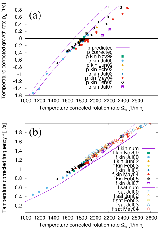
Figure 11: Growth rates (a) and frequencies (b) in the kinematic and the saturated regime for the various campaigns. The numerical predictions for the kinematic case are based on the 2D code described in the text. For the corrected curves, the effect of the finite wall thickness (determined with a 1D code) was additionally taken into account. All rotation rates, growth rates and frequencies were re-scaled to a common reference temperature of 157^∘C. Note the significant reduction of the growth rates for the two “bad” runs from July 2007.

In figure 11 we put together several numerical predictions and a rather complete set of the measured values for the growth rate $p$ and the frequency $f$. The numerically computed growth rates comes in two versions: ”p predicted” is the result of the 2D code (as discussed above), relying on the velocity measurements in water which were carried out before the sodium experiment (Christen, Hänerl & Will 1998; Stefani, Gerbeth & Gailitis 1999). ”p corrected” represents a slight correction of ”p predicted”, for which the lower conductivity of the stainless steel walls has been incorporated in the 1D-code, and the obtained corrections were then added to the 2D results (admittedly, a somewhat ”hybrid” method which seems, however, quite reliable). The corresponding two predictions for the frequencies do barely differ and are therefore summarized as one single curve ”f kin num”. The second prediction for the frequencies, ”f sat num”, concerns the values in the saturated regime. It has been obtained by solving equation (5) simultaneously with the induction equation, and inferring the frequency when the system has relaxed into saturation.

The validity of this saturation model (which gives automatically a zero growth rate) can be judged from the dependence of the resulting eigenfrequency in figure 11. We observe here a quite reasonable correspondence with the measured data, in particular with view on the slightly declined slope of the curve. A minor jump of the measured eigenfrequencies between the kinematic and the saturated regime might be attributed to the arising fluid rotation in the outermost cylinder, which is not incorporated in our simple back-reaction model.

4.2 Power increase

The excess power that is necessary to overcome the Ohmic losses due to the self-excited magnetic field is one of the most important features in the saturation regime of a dynamo. Unfortunately, its precise determination is far from trivial. One reason is that in the saturation regime it is barely possible to measure the motor power in the purely hydraulic case, without any magnetic field back-reaction, although the power in the purely hydraulic case scales over a wide range of rotation rates with the cube of the rotation rate. Yet, slightly above the critical rotation rate, where the magnetic field growth rate is slow, there are time periods long enough to determine the purely hydraulic power before the magnetic field has reached large values.

Another point is that, in particular for high rotation rates, the dynamo behaviour was not completely reproducible due to different Argon pressure regimes resulting in different couplings of the sodium flow to the propeller rotation. This means that the few available hydraulic power values in the high rotation rate region cannot be taken as an accurate reference power to compare with the full power under the action of saturated Lorentz forces. Another minor point is connected with the not perfect reproducibility of the runs, meaning that the critical rotation rate is not exactly the same for all runs. A further issue is the effect of the temperature on the conductivity.

Figure 12: Excess motor power due to the action of the Lorentz force, estimated by comparing the total power with the (not very safely determinable) pure hydraulic power.

With all those uncertainties in mind, and trying to correct for all possible inconsistencies, we inferred the dependence of the excess power on the difference of the rotation rate and the critical rotation rate. Figure 12 shows the corresponding data. Compared with the purely hydraulic power in the order of 200 kW, the typical 20 kW represent only a 10 per cent increase. This rather flat increase reflects the fluid character of the dynamo, in which the sodium flow evades and deforms under the influence of the Lorentz forces, while the resulting deterioration of the dynamo condition makes the growth rate drop down to zero.

4.3 Radial field distribution

The newly installed lances that were radially and axially movable through and along the dynamo allowed to determine the radial and axial field dependencies in much detail. Figure 13 shows the dependence of the three field components on the radius, as measured by the radial lance in the lower port. The left column shows the measured values, the right column shows the corresponding numerical predictions. While a perfect quantitative agreement cannot be expected, a nice agreement of the form of the curves is generally observed. A remarkable deviation becomes visible, however, for the $B_{\phi}(r)$ profiles at higher rotation rate, which develop a sort of ”bump” at $r=0$ which is not reflected by the numerical value.

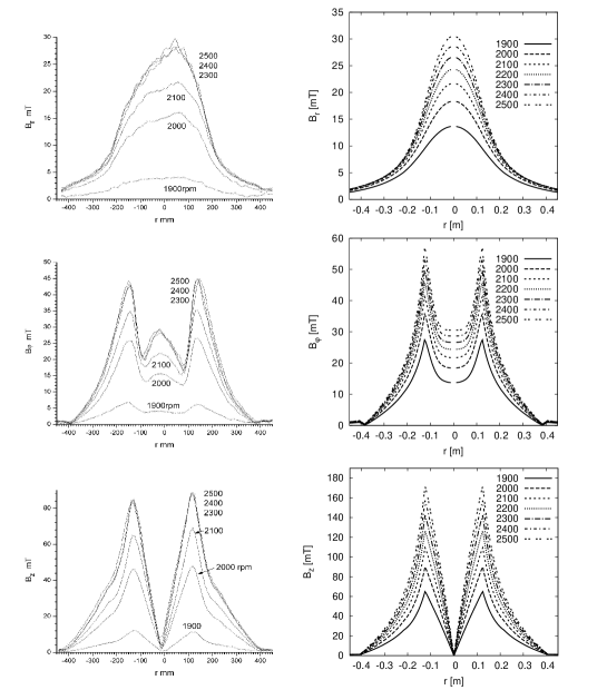
Figure 13: Radial dependencies of the three field components measured at the lower port in Run 2 from Feb 2005 (left), and corresponding numerical predictions (right).

4.4 Axial field distribution

While the radial field distribution has turned out not to change greatly from the kinematic regime to the saturation regime, the axial field is affected significantly by the back-reaction. The braking of the azimuthal velocity component, which accumulates downstream from the propeller, results in a deteriorated self-excitation capability of the flow in the lower parts of the dynamo and therefore in an upward shift of the entire magnetic field structure. This is illustrated in figure 14. First, figure 14a reiterates run 1 from June 2002 (as in figure 5), enhanced now by the signals of the sensors H2 and H6. Evidently, the ratios between the amplitudes of the upper sensor H2 and the lower sensors H4 and H6 grow with increasing rotation rates. Figure 14b shows the measured axial magnetic field amplitudes (from the same June 2002 campaign) at the upper and lower ports and their ratio in dependence on the rotation rate. The typical decrease of the ratio of lower to upper fields is also reflected in the numerical model.

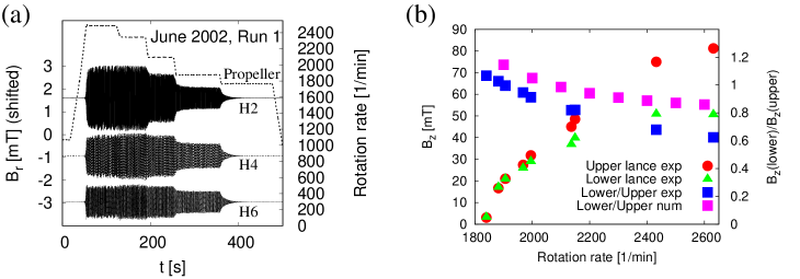
Figure 14: Upward shift of the field pattern in the saturated regime. (a) Run 1 from June 2002 (see figure 5), enhanced by the signals of H2 and H6. The amplitude ratios between the upper sensor H2 and the lower sensors H4 and H6 increase markedly for higher rotation rates (for the sake of better visibility, the signals are shifted along the ordinate axis). (b) Measured values and decreasing ratio of axial fields at the lower and upper lances. The numerical prediction for the ratio shows the same decreasing trend, although not as strong as the measured values.

4.5 Turbulence properties and magnetic field spectra

Apart from the back-reaction effects on the large scale flow structure, the effect on the fluctuations is also important. In figure 15 two spectra are shown, one from a Hall sensor which is located on the lower measurement level in the central cylinder, about 2 cm from the wall. The other spectrum results from the data of the mentioned pressure sensor, which is also mounted on the lower level. The data were recorded during run 1 of the May 2004 campaign.

Not surprisingly, the key feature of the magnetic spectrum is its peak at the eigenfrequency $f_{0}$. Yet, there are further peaks at the triple and at the five-fold frequency. Neither of these peaks is seen in the pressure spectrum. Here, we detect a dominant peak at $2f_{0}$ and some smaller peak at the $4f_{0}$. Obviously, the magnetic eigenfield with the angular mode $m=1$ produces a Lorentz force with a dominant $m=0$ part, but also with an $m=2$ part. The latter part influences the velocity and is also mirrored by the pressure peak at $2f_{0}$. Then, this $m=2$ mode of the velocity induces, together with the dominant magnetic $m=1$ mode, a new contribution with $m=3$ in the magnetic field. The product of $m=1$ and $m=3$ modes of the magnetic field produces the $m=4$ mode in the pressure. All the arguments for $m$ transfer to the multiples of the frequency since the measurement is done at a fixed position.

Concerning the inertial range of the spectrum, we have plotted a typical $f^{-11/3}$ law for the magnetic field in the inertial range and a $f^{-7/3}$ law for the pressure for comparison, without claiming perfect coincidences. Between the main field frequency $f$ and the propeller frequency $f_{prop}$ there seems to be a region with a $f^{-1}$ scaling.

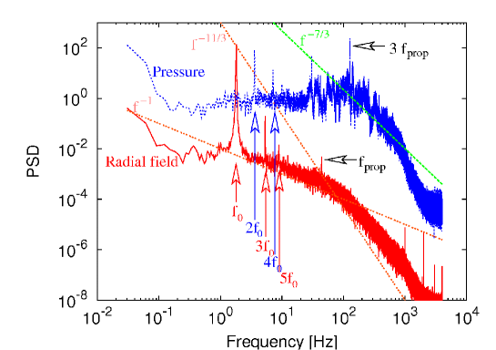
Figure 15: Spectra of the radial magnetic field and the pressure, both measured on the lower level in the inner cylinder. The pressure sensor was flash mounted to the wall. The data are for a rotation rate of 2530 rpm. The peaks are multiples of the eigenfrequency $f_{0}$ of the magnetic field. There are also peaks at the motor rotation rate and its triple value (because of three wings).

Another interesting result concerns the turbulence level. For this purpose we have analyzed the data from the June 2002 campaign. Specifically, we have used the data from the Hall sensors positioned at the upper and lower port, in the middle of the back-flow region. The sensors measure a dominant sine signal from the magnetic eigenfield whose amplitude is shown in figure 16a. The deviation from the dominant sine signal is then attributed to the flow turbulence, whose level (in per cent) is given in figure 16b. The first observation to make here is the reduced turbulence level at the upper sensors which might be due to some calming of the flow when it goes upward. The second, and more interesting observation is the general minimum of the turbulence level around 2100 rpm, for which we have no explanation up to present.

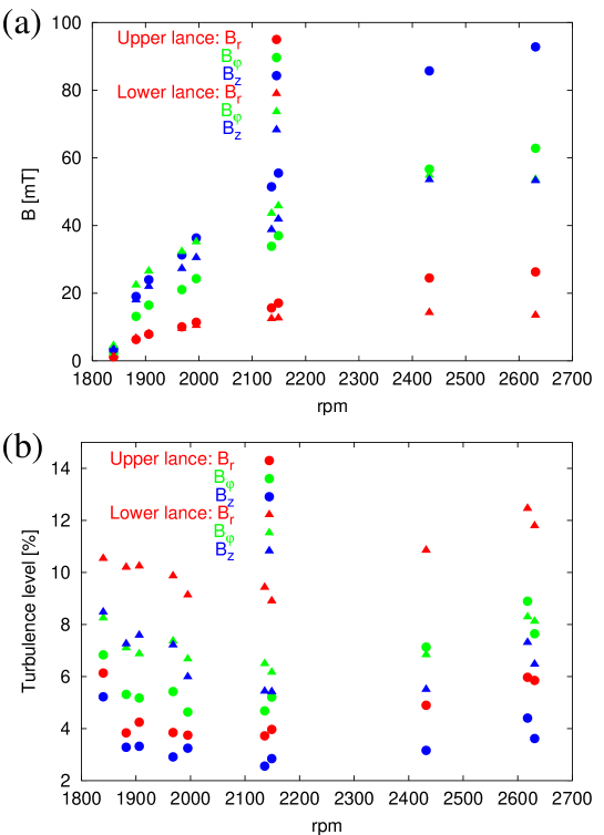
Figure 16: Amplitudes (a) and turbulence levels (b) measured in the middle of the back-flow cylinder at the lower and upper port

5 Synopsis, conclusions, prospects

Let us summarize the main results of the Riga dynamo experiments: In the kinematic regime the measured growth rates, frequencies and the spatial field structure were in close correspondence with the numerical predictions of a 2D code, in particular, when a correction for the resistive effects of the inner stainless steel walls was made. This is, actually, not a trivial point. Before the experiment was really performed, some unrecognized influence of the (low level) turbulence on the self-excitation threshold, or a greater sensitivity to the precise boundary and interface conditions, could not be ruled out entirely. Now, we can conclude that the “elementary cell” of a dynamo works robustly in the laboratory, and that its kinematic behaviour is predictable with an error margin of a few per cent.

In contrast to that, the understanding of the saturation regime is a much more involved. We have shown that a rather simple back-reaction model, which computes the selective breaking of the azimuthal flow component along the streamlines, comes close to explaining the observed back-reaction effect, such as the continuing increase of the frequency and the upward shift of the field pattern. However, there are features which are not explained by this simple model: the developing maximum of $B_{\varphi}$ at $r=0$ (see figure 13) is just a case in point. A further yet unexplained feature is the minimum of the turbulence level for some medium degree of supercriticality, as evidenced in figure 16.

After a complete disassembly, reconstruction, and refurbishment the Riga dynamo was started again with short campaigns in June 2016 and April 2017. Part of the results were published by Gailitis and Lipsbergs (2017), and further details will be discussed elsewhere. If the attainment of the old performance parameters can be confirmed, a significant modification of the flow structure is planned for the future. This is motivated by the numerical finding that a specific ”de-optimization” of the flow field in the Riga dynamo could lead to a vacillation between two states with different kinetic and magnetic energies (Stefani, Gailitis & Gerbeth 2011).

In concert with the complementary and nearly contemporaneous Karlsruhe experiment, the Riga dynamo experiment has pioneered a couple of further activities for studying dynamo action, and related magnetic instabilities, in the liquid metal lab. Important new results were, among others, the observation of magnetic field reversals in the French VKS experiment (Berhanu et al. 2010), and the experimental demonstration of the helical (Stefani et al. 2006) and azimuthal (Seilmayer et al. 2014) magnetorotational instability as well as the current-driven Tayler instability (Seilmayer et al. 2012). A comparative survey of these, and further dynamo related experiments, can be found in the review papers by Stefani, Gailitis & Gerbeth (2008) and Stefani et al. (2017).

References

- Berhanu et al. (2007) Berhanu, M. et al. 2007 Magnetic field reversals in an experimental turbulent dynamo. EPL 77, 59001.
- Christen, Hänel & Will (1998) Christen,M., Hänel, H. & Will, G. 1998 Entwicklung der Pumpe für den hydrodynamischen Kreislauf des Rigaer ”Zylinderexperimentes. In Beiträge zu Fluidenergiemaschinen 4 (ed. W.H. Faragallah & G. Grabow) pp. 111-119, Faragallah-Verlag und Bildarchiv, Sulzbach/Ts.
- Gailitis (1967) Gailitis, A. 1967 Self-excitation conditions for a laboratory model of a geomagnetic dynamo. Magnetohydrodynamics 3, No. 3, 23–29.
- Gailitis & Freibergs (1976) Gailitis, A. & Freibergs, Ya. 1976 Theory of a helical MHD dynamo. Magnetohydrodynamics 12, 127–129.
- Gailitis & Freibergs (1980) Gailitis, A. & Freibergs, Ya. 1980 Nonuniform model of a helical dynamo. Magnetohydrodynamics 16, 116–121.
- Gailitis et al. (1987) Gailitis, A. Karasev, B.G., Kirillov, I.R., Lielausis, O.A., Luzhanskii, S.M., Ogorodnikov, A.P. & Preslitskii, G.V. 1987 Experiment with a liquid-metal model of an MHD dynamo. Magnetohydrodynamics 23, 349–353.
- Gailitis (1996) Gailitis, A. 1996 Design of a liquid sodium MHD dynamo experiment. Magnetohydrodynamics 32, 58–62.
- Gailitis et al. (2000) Gailitis, A., Lielausis, O., Dement’ev, S., Platacis, E., Cifersons, A., Gerbeth, G., Gundrum, T., Stefani, F., Christen, M., Hänel, H. & Will, G. 2000 Detection of a flow induced magnetic field eigenmode in the Riga dynamo facility. Phys. Rev. Lett. 84, 4365–4368.
- Gailitis et al. (2001) Gailitis, A., Lielausis, O., Platacis, E., Dement’ev, S., Cifersons, A., Gerbeth, G., Gundrum, T., Stefani, F., Christen, M., & Will, G. 2001 Magnetic field saturation in the Riga dynamo experiment. Phys. Rev. Lett. 86, 3024–3027.
- Gailitis et al. (2001a) Gailitis, A., Lielausis, O., Platacis, E., Gerbeth, G. & Stefani, F. 2001 On the results of the Riga dynamo experiments. Magnetohydrodynamics 37, 71–79.
- Gailitis et al. (2002) Gailitis, A., Lielausis, O., Platacis, E., Gerbeth, G. & Stefani, F. 2002 Laboratory experiments on hydromagnetic dynamos. Rev. Mod. Phys. 74, 973-990.
- Gailitis et al. (2002a) Gailitis, A., Lielausis, O., Platacis, E., Dement’ev, S., Cifersons, A., Gerbeth, G., Gundrum, T., Stefani, F., Christen, M., & Will, G. 2002 Dynamo experiments at the Riga sodium facility. Magnetohydrodynamics 38, 5-14.
- Gailitis et al. (2002b) Gailitis, A., Lielausis, O., Platacis, E. Gerbeth, G. & Stefani, F. 2002 On back-reaction effects in the Riga dynamo experiment. Magnetohydrodynamics 38, 15-26.
- Gailitis et al. (2003) Gailitis, A., Lielausis, O., Platacis, E.: Gerbeth, G. & Stefani, F. 2003 The Riga dynamo experiment. Surv. Geopyhs. 24, 247-267.
- Gailitis et al. (2004) Gailitis, A., Lielausis, O., Platacis, E., Gerbeth, G. & Stefani, F. 2004 Riga dynamo experiment and its theoretical background. Phys. Plasmas 11, 2838-2843.
- Gailitis et al. (2008) Gailitis, A., Gerbeth, G., Gundrum, Th., Lielausis, O., Platacis, E. & Stefani, F. 2008 History and results of the Riga dynamo experiments. C.R. Phys. 9, 721-728.
- Gailitis & Lipsbergs (2017) Gailitis, A. & Lipsbergs, G. 2017 2016 year experiments at Riga dynamo facility, Magnetohydrodynamics 53, 349-356.
- Kenjereš et al. (2006) Kenjereš, S., Hanjalić, K., Renaudier, S., Stefani, F., Gerbeth, G. & Gailitis, A. 2006 Coupled fluid-flow and magnetic-field simulation of the Riga dynamo experiment. Phys. Plasmas 13, 122308.
- Kenjereš & Hanjalić (2007) S. Kenjereš, S. & Hanjalić, K. 2007 Numerical simulation of a turbulent magnetic dynamo. Phys. Rev Lett. 98, 104501.
- Müller & Stieglitz (2002) Müller, U. & Stieglitz, R. 2002 The Karlsruhe dynamo experiment. Nonl. Proc. Geophys. 9, 165-170.
- Müller, Stieglitz & Horanyi (2004) Müller, U., Stieglitz, R. & Horanyi, S. 2004 A two-scale hydromagnetic dynamo experiment. J. Fluid Mech. 498, 31-71.
- Müller, Stieglitz & Horanyi (2006) Müller, U., Stieglitz, R. & Horanyi, S. 2006 Complementary experiments at the Karlsruhe dynamo test facility. J. Fluid Mech. 552, 419-440.
- Steenbeck, Krause & Rädler (1966) Steenbeck, M., Krause, F. & Rädler, K.-H. 1966 Berechnung der mittleren Lorentz-Feldstärke für ein elektrisch leitendendes Medium in turbulenter, durch Coriolis-Kräfte beeinflußter Bewegung. Z. Naturforsch. 21a, 369–376.
- Steenbeck et al. (1967) Steenbeck, M., Kirko, I.M., Gailitis, A., Klawina, A.P., Krause, F., Laumanis, I.J. & Lielausis, O.A. 1967 Der experimentelle Nachweis einer elektromtorischen Kraft längs eines äußeren Magnetfeldes, induziert durch die Strömung flüssigen Metalls (-Effekt). Mber. Dt. Ak. Wiss. 9, 714–719.
- Seilmayer et al. (2012) Seilmayer, M. et al. 2012 Experimental evidence for a transient Tayler instability in a cylindrical liquid-metal column. Phys. Rev. Lett. 108, 244501.
- Seilmayer et al. (2014) Seilmayer, M. et al. 2014 Experimental evidence for nonaxisymmetric magnetorotational instability in a rotating liquid metal exposed to an azimuthal magnetic field. Phys. Rev. Lett. 113, 024505.
- Stefani, Gailitis & Gerbeth (1999) Stefani, F., Gerbeth, G. & Gailitis, A. 1999 Velocity profile optimization for the Riga dynamo experiment. In Transfer Phenomena in Magnetohydrodynamic and Electroconducting Flows, (ed. A. Alemany, Ph. Marty & J. P. Thibault), pp. 31-44, Kluwer.
- Stefani et al. (2006) Stefani, F. et al. 2006 Experimental evidence for magnetorotational instability in a Taylor-Couette flow under the influence of a helical magnetic field. Phys. Rev. Lett. 97, 184502.
- Stefani, Gailitis & Gerbeth (2008) Stefani, F., Gailitis, A., Gerbeth, G. 2008 Magnetohydrodynamic experiments on cosmic magnetic fields. ZAMM 88, 930-954.
- Stefani, Giesecke & Gerbeth (2009) Stefani, F., Giesecke, A., Gerbeth, G. 2009 Numerical simulations of liquid metal experiments on cosmic magnetic fields. Theor. Comp. Fluid Dyn. 23, 405-429.
- Stefani, Gailitis & Gerbeth (2011) Stefani, F., Gailitis, A. & Gerbeth, G. 2011 Energy oscillations and a possible route to chaos in a modified Riga dynamo. Astron. Nachr. 332, 4–10.
- Stefani et al. (2017) Stefani, F. et al. 2017 Magnetic field dynamos and magnetically triggered flow instabilities. IOP Conf. Ser.: Mater. Sci. Eng. 228, 012002.
- Stieglitz & Müller (2001) Stieglitz, R., Müller, U 2001 Experimental demonstration of a homogeneous two- scale dynamo. Phys. Fluids 13, 561–564.