Complexity of viscous dissipation in turbulent thermal convection

Abstract

Using direct numerical simulations of turbulent thermal convection for Rayleigh number ($\mathrm{Ra}$) between $10^{6}$ and $10^{8}$ and unit Prandtl number, we derive scaling relations for viscous dissipation in the bulk and in the boundary layers. We show that contrary to the general belief, the total viscous dissipation in the bulk is larger, albeit marginally, than that in the boundary layers. The bulk dissipation rate is similar to that in hydrodynamic turbulence with log-normal distribution, but it differs from $(U^{3}/d)$ by a factor of $\mathrm{Ra}^{-0.18}$. Viscous dissipation in the boundary layers are rarer but more intense with a stretched-exponential distribution.

Physics of hydrodynamic turbulence is quite complex, involving strong nonlinearity and boundary effects. To simplify, researchers have considered hydrodynamic turbulence in box away from the walls. The turbulence in such a geometry is statistically homogeneous and isotropic. The physics of such idealised flows too remain primarily unsolved, yet their energetics is reasonably well understood. Here, the energy supplied at large length scales cascades to intermediate scales, and then to dissipative scales Kolmogorov (1941a, b). Thus, under steady state, the energy supplied by the external force equals the energy cascade rate, $\Pi_{u}$, and the viscous dissipation rate, $\epsilon_{u}$. From dimensional analysis it has been deduced that $\epsilon_{u}\approx U^{3}/L$, where $U$ is the large-scale velocity, $L$ is the large length scale, and the prefactor is approximately unity McComb (1990); Lesieur (2008).

Thermal convection is a very important problem of science and engineering. Here too researchers have considered an idealised system called Rayleigh–Bénard convection (RBC) in which a fluid is confined between two horizontal thermal plates separated by a vertical distance of $d$; the bottom plate is hotter than the top one Ahlers, Grossmann, and Lohse (2009); Lohse and Xia (2010); Verma, Kumar, and Pandey (2017). The kinematic viscosity ($\nu$) and thermal diffusivity ($\kappa$) are treated as constants. Additionally, the density of the fluid is considered to be a constant except for the buoyancy term of the fluid equation. The governing equations of RBC are as follows:

$$\partial_{t}\mathbf{u}+(\mathbf{u}\cdot\nabla)\mathbf{u} = -\nabla\sigma/\rho_{0}+\alpha g\theta\hat{z}+\nu\nabla^{2}\mathbf{u},$$ (1)

$$\partial_{t}\theta+(\mathbf{u}\cdot\nabla)\theta = (\Delta/d)u_{z}+\kappa\nabla^{2}\theta,$$ (2)

$$\nabla\cdot\mathbf{u} = 0,$$ (3)

where $\mathbf{u}$ and $\sigma$ are the velocity and pressure fields respectively, $\theta$ is temperature fluctuation over the conduction state, $\rho_{0}$ and $\alpha$ are respectively the mean density and thermal expansion coefficient of the fluid, $g$ is acceleration due to gravity, and $\Delta$ is the temperature difference between the hot and cold plates. RBC is specified by two nondimensional parameters—Rayleigh number $\mathrm{Ra}=(\alpha g\Delta d^{3})/(\nu\kappa)$, which is a measure of buoyancy, and the Prandtl number $\mathrm{Pr}=\nu/\kappa$ (see supplementary material).

For thermal convection, walls and their associated boundary layers play an important role, hence turbulence in thermal convection is more complex than hydrodynamic turbulence. In this Letter, we focus on the properties of the viscous dissipation in RBC. Verzicco and Camussi (2003) and Zhang, Zhou, and Sun (2017) computed the viscous dissipation rates in the bulk and in the boundary layers in RBC, and found them to be of the same order. Here, we perform a detailed analysis of these quantities and their probability distributions, both numerically and phenomenologically. We will show that the walls of thermally-driven turbulence introduce interesting and generic features in the viscous dissipation.

Shraiman and Siggia (1990) derived an interesting exact relation that relates the viscous dissipation rate, $\epsilon_{u}$, to the heat flux:

$$\epsilon_{u}=\left\langle\epsilon_{u}(\mathbf{r})\right\rangle=\left\langle\frac{\nu}{2}\left(\frac{\partial u_{i}}{\partial x_{j}}+\frac{\partial u_{j}}{\partial x_{i}}\right)^{2}\right\rangle\\ =\frac{\nu^{3}}{d^{4}}\frac{\mathrm{(Nu-1)Ra}}{\mathrm{Pr}^{2}}=\frac{U^{3}}{d}\frac{\mathrm{(Nu-1)Ra}}{\mathrm{Re}^{3}\mathrm{Pr}^{2}},$$ (4)

where $\langle\,\rangle$ denotes the volume average over the entire domain, and $u_{i}$ with $i=(x,y,z)$ is the $i$th the component of the velocity field. The Nusselt number, $\mathrm{Nu}$, is the ratio of the total heat flux and the conductive heat flux, and $\mathrm{Re}=UL/\nu$ is the Reynolds number. When the boundary layer is either absent (as in periodic box) or weak (as in the ultimate regime proposed by Kraichnan Kraichnan (1962)), $\mathrm{Nu}\sim(\mathrm{RaPr})^{1/2}$ and $\mathrm{Re}\sim(\mathrm{Ra/Pr})^{1/2}$ (See Refs.Grossmann and Lohse (2000, 2001); Verma et al. (2012); Verma, Kumar, and Pandey (2017)). Substitution of these relations in Eq. (4) yields $\epsilon_{u}\sim U^{3}/d$, similar to hydrodynamic turbulence. In this Letter we focus on $\mathrm{Pr}\sim 1$, hence we ignore the Prandtl number dependence.

The scaling however is different for realistic RBC for which boundary layers near the plates play an important role. Scaling arguments Malkus (1954); Castaing et al. (1989); Grossmann and Lohse (2000, 2002), experiments Castaing et al. (1989); Qiu and Tong (2002); Brown, Funfschilling, and Ahlers (2007); Funfschilling et al. (2005); Nikolaenko et al. (2005); Ahlers, Grossmann, and Lohse (2009) and numerical simulations Verzicco and Camussi (2003); Stringano and Verzicco (2006); Scheel, Kim, and White (2012); Scheel and Schumacher (2014); Pandey et al. (2016); Pandey and Verma (2016) reveal that $\mathrm{Re}\sim\mathrm{Ra}^{1/2}$ and $\mathrm{Nu}\sim\mathrm{Ra}^{0.3}$, substitution of which in Eq. (4) yields $\epsilon_{u}\neq U^{3}/d$, rather

$$\epsilon_{u}\sim\frac{U^{3}}{d}\mathrm{Ra}^{-0.2}\sim\frac{\nu^{3}}{d^{4}}\mathrm{Ra}^{1.3},$$ (5)

because $U\sim\mathrm{Re}\sim\mathrm{Ra}^{1/2}$. This is due to the relative suppression of the nonlinear interactions in RBC, as Pandey et al. (2016); Pandey and Verma (2016); Verma, Kumar, and Pandey (2017) showed that in RBC, the ratio of the nonlinear term and viscous term scales as $(UL/\nu)\mathrm{Ra}^{-0.15}$. The aforementioned suppression of nonlinear interactions leads to weaker energy cascade $\Pi(k)$, and hence lower viscous dissipation than the corresponding hydrodynamic turbulence.

In RBC, the viscous dissipation rates in the bulk and in the boundary layers are very different. In the following discussion, using scaling arguments and the exact relation given by Eq. (4), we will quantify the total viscous dissipation rates in the bulk and boundary layers, $\tilde{D}_{u,\mathrm{bulk}}$ and ${\tilde{D}_{u,\mathrm{BL}}}$, as well as the corresponding average viscous dissipation rates, $\epsilon_{u,\mathrm{bulk}}$ and $\epsilon_{u,\mathrm{BL}}$, which are obtained by dividing the total dissipation rates by their respective volumes.

Grossmann and Lohse’s model Grossmann and Lohse (2000, 2001) assumes that $\epsilon_{u,\mathrm{bulk}}\sim U^{3}/d\sim\mathrm{Ra}^{3/2}$. We find that the average viscous dissipation in the bulk scales similar to the viscous dissipation rate in the entire volume, i.e.,

$$\epsilon_{u,\mathrm{bulk}}\sim\frac{U^{3}}{d}\mathrm{Ra}^{-0.18}.$$ (6)

Since the fluid flow in the boundary layers is laminar, we expect $\epsilon_{u,\mathrm{BL}}\sim\nu U^{2}/\delta_{u}^{2}$, where $\delta_{u}$ is the thickness of the viscous boundary layer. Hence, the ratio of the two dissipation rates is

$$\frac{\epsilon_{u,\mathrm{BL}}}{\epsilon_{u,\mathrm{bulk}}} \sim \mathrm{Ra}^{0.18}\left(\frac{\nu U^{2}}{\delta_{u}^{2}}\right)/\left(\frac{U^{3}}{d}\right)$$ (7)

$$\sim \frac{1}{\mathrm{Re}}\left(\frac{d}{\delta_{u}}\right)^{2}\mathrm{Ra}^{0.18}\sim\left(\frac{d}{\delta_{u}}\right)^{2}\mathrm{Ra}^{-0.32}.$$

Note however that the volume of the boundary layers is much less than that of the bulk. For simplicity, we assume that the fluid is contained in a cube of dimension $d$, then the ratio of the volumes of the boundary layer and bulk is

$$\frac{V_{\mathrm{BL}}}{V_{\mathrm{bulk}}}\sim\frac{\delta_{u}d^{2}}{(d-\delta_{u})^{3}}\sim\frac{\delta_{u}}{d},$$ (8)

because $\delta_{u}\ll d$ for $\mathrm{Pr}\sim 1$. Using the above relations, we can deduce the scaling of the ratio of the total viscous dissipation rates in the boundary layer and in the bulk as

$$\frac{\tilde{D}_{u,\mathrm{BL}}}{\tilde{D}_{u,\mathrm{bulk}}} \sim \frac{\epsilon_{u,\mathrm{BL}}}{\epsilon_{u,\mathrm{bulk}}}\times\frac{V_{\mathrm{BL}}}{V_{\mathrm{bulk}}}\sim\frac{d}{\delta_{u}}\mathrm{Ra}^{-0.32}.$$ (9)

According to Prandtl–Blassius theory Schlichting and Gersten (2000),

$$\frac{\delta_{u}}{d}\sim\mathrm{Re}^{-1/2}\sim\mathrm{Ra}^{-1/4},$$ (10)

which yields $\tilde{D}_{u,\mathrm{BL}}/\tilde{D}_{u,\mathrm{bulk}}\sim\mathrm{Ra}^{-0.07}$. Thus, in RBC, the total viscous dissipation in the boundary layer and bulk are comparable to each other. For very large $\mathrm{Ra}$, the bulk dissipation outweighs the dissipation in the boundary layer. This is contrary to the general belief that the viscous dissipation occurs primarily in the plumes of the boundary layers.

In this Letter, using numerical simulations we show that $\delta_{u}/d$ differs slightly from Eq. (10), and

$$\frac{\delta_{u}}{d}\sim\mathrm{Re}^{-0.44}\sim(\mathrm{Ra}^{1/2})^{-0.44}\sim\mathrm{Ra}^{-0.22},$$ (11)

using which we find

$$\frac{\tilde{D}_{u,\mathrm{BL}}}{\tilde{D}_{u,\mathrm{bulk}}}\sim\mathrm{Ra}^{-0.10}.$$ (12)

Thus,

$$\epsilon_{u,\mathrm{BL}} \sim \frac{\nu U^{2}}{\delta_{u}^{2}}\sim\frac{\nu^{3}}{d^{4}}\mathrm{Ra}^{1.44},$$ (13)

$$\tilde{D}_{u,\mathrm{BL}} \sim \epsilon_{u,\mathrm{BL}}\,\delta_{u}d^{2}\sim\frac{\nu^{3}}{d}\mathrm{Ra}^{1.22},$$ (14)

$$\tilde{D}_{u,\mathrm{bulk}} \sim \epsilon_{u,\mathrm{bulk}}\,d^{3}\sim\frac{\nu^{3}}{d}\mathrm{Ra}^{1.32}.$$ (15)

Interestingly, $\tilde{D}_{u,\mathrm{BL}}\sim d^{2}\nu U^{2}/\delta_{u}\sim(\nu^{3}/d)\mathrm{Ra}^{5/4}$, as assumed in Grossmann and Lohse’s model Grossmann and Lohse (2000, 2001).

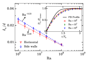
Figure 1: Plot of normalized boundary layer thickness $\delta_{u}/d$ vs. $\mathrm{Ra}$ for horizontal and vertical plates. Best fits are depicted as dashed and dotted lines. Inset shows the comparison of horizontal velocity profiles near the bottom plate with the Prandtl–Blasius profile (solid black line).

Table 1: Details of our direct numerical simulations performed in a unit box for $\mathrm{Pr}=1$: the Rayleigh Number (Ra), the kinematic viscosity ($\nu$), the Reynolds Number (Re), the ratio of the Kolmogorov length scale ($\eta$) to the average mesh width $\Delta x_{\mathrm{avg}}$, the Nusselt Number (Nu), the Nusselt number deduced from $\epsilon_{u}$ using Eq. (4) ($\mathrm{Nu_{S}}$), number of mesh points in the viscous boundary layer ($N_{\mathrm{BL}}$), volume fraction of the boundary layer region ($V_{\mathrm{BL}}/V$), and the ratio $\tilde{D}_{u,\mathrm{BL}}/\tilde{D}_{u,\mathrm{bulk}}$.

$\mathrm{Ra}$	$\nu(=\kappa)$	$\mathrm{Re}$	$\eta/\Delta x_{\mathrm{avg}}$	$\mathrm{Nu}$	$\mathrm{Nu_{S}}$	$N_{\mathrm{BL}}$	$V_{\mathrm{BL}}/V$	$\tilde{D}_{u,\mathrm{BL}}/\tilde{D}_{u,\mathrm{bulk}}$
$\mathrm{1\times 10^{6}}$	$0.001$	$\mathrm{150}$	$4.92$	$\mathrm{8.40}$	$8.34$	$10$	$0.14$	$0.81$
$\mathrm{2\times 10^{6}}$	$0.0007071$	$\mathrm{212}$	$3.89$	$10.1$	$10.3$	$8$	$0.12$	$0.67$
$\mathrm{5\times 10^{6}}$	$0.0004472$	$\mathrm{342}$	$2.87$	$\mathrm{13.3}$	$13.5$	$7$	$0.099$	$0.65$
$\mathrm{1\times 10^{7}}$	$0.00032$	$\mathrm{460}$	$2.32$	$\mathrm{16.0}$	$15.9$	$6$	$0.086$	$0.63$
$\mathrm{2\times 10^{7}}$	$0.0002236$	$\mathrm{654}$	$1.84$	$\mathrm{20.0}$	$20.0$	$5$	$0.074$	$0.61$
$\mathrm{5\times 10^{7}}$	$0.0001414$	$\mathrm{1080}$	$1.36$	$\mathrm{25.5}$	$26.0$	$4$	$0.062$	$0.57$
$\mathrm{1\times 10^{8}}$	$0.0001$	$\mathrm{1540}$	$1.09$	$\mathrm{32.8}$	$32.0$	$4$	$0.054$	$0.56$

We perform direct numerical simulation of RBC and verify the aforementioned scaling. The simulations were performed using a finite volume code OpenFOAM Jasak et al. (2007) for $\mathrm{Pr}=1$ and Ra between $10^{6}$ and $10^{8}$ in a three-dimensional cube of unit dimension. We impose no-slip boundary condition at all the walls, isothermal condition at the top and bottom walls, and adiabatic condition at the sidewalls (see supplementary material). Second-order Crank-Nicolson scheme is used for time-stepping. The values of $\nu$ and $\kappa$ used in the simulations are shown in Table 1, while keeping the temperature difference between the horizontal plates $\Delta=1$ for all the runs.

We employ $256^{3}$ non-uniform grid points and solve the governing equations of RBC. The grid is finer near the walls so as to adequately resolve the boundary layer. We ensure that minimum 4 grid points are in the boundary layer, thereby satisfying the criterion set by Grötzbach (1983). The ratio of the Kolmogorov length scale $\eta$ to the average mesh width $\Delta x_{\mathrm{avg}}$ remains greater than unity for each simulation run implying that the smallest length scales are being adequately resolved in our simulations. We observe that the Nusselt numbers computed numerically using $\langle u_{z}\theta\rangle$ match quite closely with those computed using $\epsilon_{u}$ and Eq. (4). See Table 1 for the comparison of these two Nusselt numbers. Also, to validate our code, we compute Nu for $\mathrm{Pr=6.8}$ fluid and verify that it matches quite well with the experimental value of Nu Zhou et al. (2012). We further remark that our simulations capture the large-scale quantities—volume-averaged viscous dissipation and Nusselt number—quite well; such quantities are not affected significantly by discretization errors at very small scales. Note that spectral method is more accurate but more complex than a finite volume method; yet a sufficiently-resolved finite volume code is quite appropriate for studying large-scale quantities.

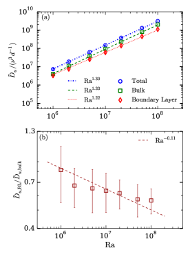
Figure 2: (a) Plots of the viscous dissipation rates $\tilde{D}_{u}$—total, bulk, and in the boundary layer—vs. $\mathrm{Ra}$. (b) Plot of the dissipation rate ratio, $\tilde{D}_{u,\mathrm{BL}}/\tilde{D}_{u,\mathrm{bulk}}$, vs. Ra that varies as $\mathrm{Ra}^{-0.11}$.

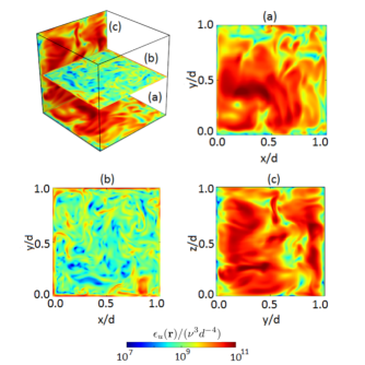
Figure 3: For $\mathrm{Ra}=10^{8}$: Spatial distribution of normalized viscous dissipation rate $\epsilon_{u}({\bf r})/(\nu^{3}d^{-4})$ in planes (a) in the bottom boundary layer at $z=2\delta_{u}/3$, (b) in the bulk at $z=0.5d$, and (c) in one of the sidewall boundary layers at $x=2\delta_{u}/3$.

First we compute the thickness of the boundary layer, $\delta_{u}$, for all our runs. For the same, we compute the root mean square horizontal velocity in each horizontal plane and estimate $\delta_{u}$ as the vertical height of the intersection of the tangent to the profile at its local maximum with the slope of the profile at the plates Qiu and Xia (1998); Scheel, Kim, and White (2012); Shi, Emran, and Schumacher (2012). Similar computations are performed for the side walls. In Fig. 1 we plot $\delta_{u}$ for the horizontal and side walls. The best fit curves of the data yield

At thermal plates: $$\delta_{u}/d=0.35\mathrm{Ra}^{-0.20},$$ (16)

At sidewalls: $$\delta_{u}/d=0.62\mathrm{Ra}^{-0.23},$$ (17)

Average: $$\delta_{u}/d=0.52\mathrm{Ra}^{-0.22},$$ (18)

with the errors in the exponents and prefactors being $\approx 0.002$ and 0.01 respectively. In Fig. 1, we plot the horizontal and sidewall boundary layer thicknesses against Ra. These results, a key ingredient of our scaling arguments [see Eq. (11)], are consistent with earlier works Verzicco and Camussi (1999, 2003); Scheel, Kim, and White (2012). As shown in the inset of Fig. 1, near the wall, the velocity profiles differ slightly from the Prandtl–Blasius profile, a result consistent with those of Scheel, Kim, and White (2012) and Shi, Emran, and Schumacher (2012); such deviations are attributed to the perpetual emission of plumes from the thermal boundary layers.

We compute the ratio $V_{\mathrm{BL}}/V$, where $V$ is the total volume, using $\delta_{u}$ and Eq. (8). In Table 1, we list this ratio for various Ra’s. Clearly, the boundary layer occupies much less volume than the bulk, and the ratio decreases with Ra as $\delta_{u}/d\propto\textrm{Ra}^{-0.22}$ [see Eq. (11)].

After this, from the numerical data we compute the total dissipation rates in the bulk and in the boundary layer by computing $\int d\tau\epsilon_{u}(\mathbf{r})$ over the respective volumes. In Fig. 2(a), we plot these values for various Ra’s. Best fit curves for these data sets yield

$$\tilde{D}_{u,\mathrm{bulk}} \approx 0.05\frac{\nu^{3}}{d}\mathrm{Ra}^{1.33},$$ (19)

$$\tilde{D}_{u,\mathrm{BL}} \approx 0.2\frac{\nu^{3}}{d}\mathrm{Ra}^{1.22},$$ (20)

which are consistent with the scaling arguments presented in Eqs. (14, 15). The ratio of the above quantities, plotted in Fig. 2(b) and listed in Table 1, is

$$\frac{\tilde{D}_{u,\mathrm{BL}}}{\tilde{D}_{u,\mathrm{bulk}}}\approx 4\mathrm{Ra}^{-0.11},$$ (21)

which is consistent with the scaling of Eq. (12). Note that the above ratio, listed in Table 1, decreases from 0.81 to 0.56 as Ra is increased from $10^{6}$ to $10^{8}$. Thus, bulk dissipation dominates the dissipation in the boundary layer, which is contrary to the belief that viscous dissipation primarily takes place in the boundary layer. It is however important to keep in mind that the scaling arguments take inputs from numerical simulations, such as Eq. (18) and Nusselt number scaling.

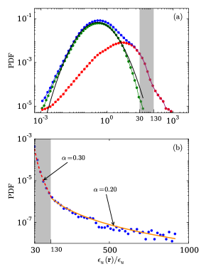
Figure 4: For $\mathrm{Ra}=10^{8}$ and $\mathrm{Pr}=1$: (a) Probability distribution functions (PDF) of normalized local dissipation rate $\epsilon_{u}$ in the bulk (green), in the boundary layer (red), and in the entire volume (blue). The bulk $\epsilon_{u}$ has a log-normal distribution (solid black line) with $\sigma=1.2$ and $\mu=0.4$. (b) Semilog plot of the PDF of $\epsilon_{u}$ indicates strong tail for $\epsilon_{u,\mathrm{BL}}$ that fits well with a stretched exponential curve with $\alpha=0.30$ (dashed red line) in the shaded region, and with $\alpha=0.20$ (solid orange line) outside the region. The shaded region is also shown in (a) for comparison.

Thus, both scaling arguments and numerical simulations show that the bulk dissipation is weaker than that in hydrodynamic turbulence, for which $\tilde{D}_{u,\mathrm{bulk}}\sim U^{3}/d\sim\mathrm{Ra}^{3/2}$. We also compute the total dissipation rate in volume $V_{i}=(1/4)^{3}V$ located deep inside the bulk, and observe similar weak scaling with Ra (see supplementary material). Further, the viscous dissipation in the bulk dominates that in the boundary layer, albeit marginally. The boundary layer however occupies much smaller volume than the bulk. Hence, $\epsilon_{u}({\bf r})$ in the boundary layer is much more intense than in the bulk, which is illustrated in Fig. 3. Here we show density plots of normalized viscous dissipation rate $\epsilon_{u}({\bf r})/(\nu^{3}d^{-4})$ for three planes—in the bottom and a side boundary layer, and in the bulk.

To quantify the asymmetry of the dissipation rate in the bulk and in the boundary layer, for $\mathrm{Ra}=10^{8}$, we compute the probability distribution function (PDF) of local viscous dissipation, $\epsilon_{u}({\bf r})$, over the full volume, the bulk, and the boundary layer. These PDFs, plotted in Fig. 4, reveal many important features. Note that $\epsilon_{u}({\bf r})=d\tilde{D}_{u}/d\tau$ with $d\tau$ as the local volume. For $\epsilon_{u}({\bf r})/\epsilon_{u}<20$, we observe that $\epsilon_{u,\mathrm{bulk}}({\bf r})\gg\epsilon_{u,\mathrm{BL}}({\bf r})$, thus average dissipation rate in the bulk is relatively weak. But for $\epsilon_{u}({\bf r})/\epsilon_{u}>20$, the viscous dissipation in the boundary layer dominates the bulk dissipation.

In addition, the PDF of $\epsilon_{u,\mathrm{bulk}}$ is log-normal, similar to Obukhov’s predictions Obukhov (1962) for the hydrodynamic turbulence. See Fig. 4(a) for an illustration. This is consistent with the results of Kumar, Chatterjee, and Verma (2014) and Verma, Kumar, and Pandey (2017), who showed similarities between turbulence in RBC and in hydrodynamics. The PDF of $\epsilon_{u,\mathrm{BL}}$ however is given by a stretched exponential—$P(\epsilon_{u})\sim\beta\exp(-m\epsilon_{u}^{*\alpha})/\sqrt{\epsilon_{u}^{*}}$ with $\alpha\approx 0.20$ for $\epsilon_{u}(\mathbf{r})/\epsilon_{u}>130$ and $\alpha\approx 0.30$ for $30<\epsilon_{u}(\mathbf{r})/\epsilon_{u}<130$ [see Fig. 4(b)]. Here $\epsilon^{*}_{u}$ correspond to those values of $\epsilon_{u}$, which are larger than the abscissa of the most probable value. This result indicates that the extreme dissipation takes place inside the boundary layer. We also carry out the PDF analysis of $\epsilon_{u,\mathrm{BL}}$ for $\mathrm{Ra}=10^{6}$ and $10^{7}$ and observe similar findings (see supplementary material). Our detailed work is consistent with earlier results Verzicco and Camussi (2003); Zhang, Zhou, and Sun (2017). Emran and Schumacher (2008) reported similar PDF for the thermal dissipation rate.

We remark that by conducting a similar analysis for Pr = 6.8 and moderate Rayleigh numbers, we observe nearly identical scaling behaviour and distribution of viscous dissipation rate (see supplementary material). Thus, it can be inferred that our findings are robust.

A combination of scaling and PDF results reveals that the local viscous dissipation in the bulk, $\epsilon_{u,\mathrm{bulk}}({\bf r})$ is weak, but they add up to a significant sum due to a larger volume. On the contrary, boundary layer exhibits extreme dissipation in a smaller volume. Interestingly, the total dissipation rate in the bulk and in the boundary layers are comparable, with bulk dominating the boundary layer marginally.

Our findings clearly contrast the homogeneous-isotropic hydrodynamic turbulence and thermally-driven turbulence. The dissipation in thermal convection has two components—$\epsilon_{u,\mathrm{bulk}}$ similar to hydrodynamic turbulence, but distinctly weaker by a factor of $\mathrm{Ra}^{-0.18}$; and $\epsilon_{u,\mathrm{BL}}$, which is unique to the flows with walls. We believe that a similar approach could be employed to analyse the thermal dissipation rate and heat transport.

See supplementary material for a similar analysis of viscous dissipation for a larger Prandtl number $\mathrm{Pr=6.8}$ and the Rayleigh number dependence of the probability distribution function.

We thank S. Fauve, R. Lakkaraju, M. Anas, and R. Samuel for useful discussions. Our numerical simulations were performed on Shaheen II at Kaust supercomputing laboratory, Saudi Arabia, under the project k1052. This work was supported by the research grants PLANEX/PHY/2015239 from Indian Space Research Organisation, India, and by the Department of Science and Technology, India (INT/RUS/RSF/P-03) and Russian Science Foundation Russia (RSF-16-41-02012) for the Indo-Russian project.

References

- Kolmogorov (1941a) A. N. Kolmogorov, “The local structure of turbulence in incompressible viscous fluid for very large Reynolds numbers,” Dokl Acad Nauk SSSR 30, 301–305 (1941a).
- Kolmogorov (1941b) A. N. Kolmogorov, “Dissipation of Energy in Locally Isotropic Turbulence,” Dokl Acad Nauk SSSR 32, 16–18 (1941b).
- McComb (1990) W. D. McComb, The physics of fluid turbulence, Oxford engineering science series (Clarendon Press, Oxford, 1990).
- Lesieur (2008) M. Lesieur, Turbulence in Fluids (Springer-Verlag, Dordrecht, 2008).
- Ahlers, Grossmann, and Lohse (2009) G. Ahlers, S. Grossmann, and D. Lohse, “Heat transfer and large scale dynamics in turbulent Rayleigh-Bénard convection,” Rev. Mod. Phys. 81, 503–537 (2009).
- Lohse and Xia (2010) D. Lohse and K. Q. Xia, “Small-scale properties of turbulent Rayleigh–Bénard convection,” Annu. Rev. Fluid Mech. 42, 335–364 (2010).
- Verma, Kumar, and Pandey (2017) M. K. Verma, A. Kumar, and A. Pandey, “Phenomenology of buoyancy-driven turbulence: recent results,” New J. Phys. 19, 025012 (2017).
- Verzicco and Camussi (2003) R. Verzicco and R. Camussi, “Numerical experiments on strongly turbulent thermal convection in a slender cylindrical cell,” J. Fluid Mech. 477, 19–49 (2003).
- Zhang, Zhou, and Sun (2017) Y. Zhang, Q. Zhou, and C. Sun, “Statistics of kinetic and thermal energy dissipation rates in two-dimensional turbulent Rayleigh–Bénard convection,” J. Fluid Mech. 814, 165–184 (2017).