Hypothesis testing of scientific Monte Carlo calculations

Abstract

The steadily increasing size of scientific Monte Carlo simulations and the desire for robust, correct, and reproducible results necessitates rigorous testing procedures for scientific simulations in order to detect numerical problems and programming bugs. However, the testing paradigms developed for deterministic algorithms have proven to be ill suited for stochastic algorithms. In this paper we demonstrate explicitly how the technique of statistical hypothesis testing, which is in wide use in other fields of science, can be used to devise automatic and reliable tests for Monte Carlo methods, and we show that these tests are able to detect some of the common problems encountered in stochastic scientific simulations. We argue that hypothesis testing should become part of the standard testing toolkit for scientific simulations.

I Introduction

Scientific computing, i.e., the process of obtaining numerical results from scientific theories using algorithms, relies on correct and reproducible implementations of computer programs. In condensed matter and statistical physics, these computer programs were traditionally small, often implemented by a single researcher, and tested and debugged by hand until no more problems could be found.

Over time, the size and complexity of programs in this field has grown rapidly. For example, computer programs for complex many-body problems, such as finding the ground state energy of an interacting solid Kim et al. (2012) or evaluating response functions of correlated quantum impurity models Gaenko et al. (2017); Parcollet et al. (2015), now span hundreds of thousands of lines that are developed and maintained by large and constantly changing teams. For such programs, manual testing becomes inefficient and expensive.

This challenge is not unique to scientific computing, and software engineering has responded by establishing automated testing practices. The corresponding arsenal of methods includes, in order of increasing granularity: contract programming, where invariants in the program state are verified continuously during execution Meyer (1992); unit tests, which ensure the correctness of small sections of the code Binder (2000); as well as integration and system tests, which check that implementations yield correct non-trivial results for predefined benchmark problems British Computer Society Working Group on Testing (1986).

These techniques have permeated scientific software engineering Dubois (2005), and they are by now standard in many computational science packages. Combined with continuous testing, i.e., the automatic execution of tests after a change to the code base, they have led to a massive improvement of the quality and resilience of scientific software Sanders and Kelly (2008).

Nevertheless, there is a large part of computational and statistical physics where such tests were so far not practical, namely the field of stochastic Monte Carlo simulations. In this domain, results make use of random or pseudo-random number generators, and are therefore intrinsically stochastic in nature. Agreement with a reference result has to be “within error bars” only.

As far as we are aware, most practitioners of these techniques therefore either enforce a deterministic procedure (e.g., a simulation with a fixed seed of the pseudo-random number generator or an otherwise fixed sequence of updates on a given configuration) or resort to “visual inspection” of the results to determine agreement between simulation and reference, neither of which is optimal. The former breaks whenever the sequence or ratio of updates are changed, and therefore is prone to false negatives, i.e., failed tests even though the results are correct. The latter relies on human intervention and is therefore neither reliable nor automatable.

In this paper, we show how tools of statistics Stuart et al. (2010), known for more than a century and in wide use in many fields, should be used to construct automated tests for physics simulations. Our formulations are general and applicable to any stochastic simulation. While we are not aware of applications to physics so far, we emphasize that similar applications have been pioneered both in the field of image synthesis Ševčíková et al. (2006) and urban simulations Subr and Arvo (2007).

In the remainder of this paper we will introduce the concept of statistical testing or “hypothesis testing” in Sec. II and III, with applications to the two-dimensional Ising model. Sec. IV shows an application to the Anderson impurity model, and Sec. V summarizes our conclusions.

II Scalar Tests

II.1 One-sample test for the mean

The basic idea of statistical hypothesis testing in the context of Monte Carlo is straight-forward: one first chooses a model for which an exact benchmark result $y$ exists. The null hypothesis, $H_{0}$, is that there is no significant difference between this reference result and the expectation value $\mathrm{E}[\hat{X}]$ of a simulation with the estimator $\hat{X}$ Subr and Arvo (2007). The alternate hypothesis, $H_{1}$, is that this is not the case:

$$H_{0} :\mathrm{E}[\hat{X}]=y$$ (1a)

$$H_{1} :\mathrm{E}[\hat{X}]\neq y.$$ (1b)

We first discuss the scalar case. Let $\hat{X}$ be a “simple” Monte Carlo estimator, i.e., an average $\langle X\rangle$ over $N$ independent random variables identically distributed according to $X$. (In the case of sampling on a Markov chain, one has to correct the number $N^{\prime}$ of Monte Carlo samples by the integrated autocorrelation time: $N=N^{\prime}/\tau_{\mathrm{int},X}$.) We then find:

$$\frac{\langle X\rangle-y}{\sigma_{X}/\sqrt{N}}\sim t_{N-1},$$ (2)

where $\sim$ is shorthand for “is distributed according to”, $t_{\nu}$ is Student’s $t$ distribution for $\nu$ degrees of freedom and $\sigma_{X}^{2}$ is the variance of $X$.

Following standard practice Neyman and Pearson (1933), we turn Eq. (2) into a likelihood estimate for $H_{0}$, known as Student’s $t$ test. We compute the two-sided $p$-value as $p=2P^{-1}(-|z|)$, where $P^{-1}$ is the inverse of the cumulative distribution function of the right-hand side and $z$ is the observed left-hand side in Eq. (2). Finally, we compare $p$ with a significance level $\alpha\in(0,1)$ and reject the null hypothesis (1a) if $p<\alpha$. In other words, the $p$ value is the probability of observing $z$ or a “more unlikely” event given $H_{0}$, and we reject the $H_{0}$ if that probability becomes smaller than $\alpha$.

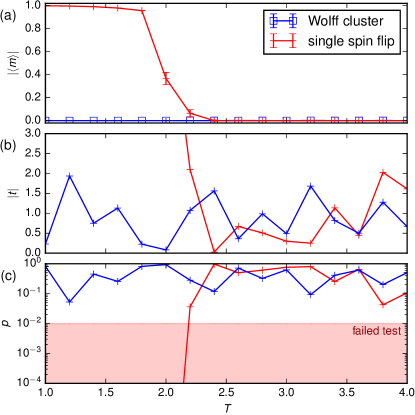
Figure 1: Scalar one-sample test against $\langle m\rangle=0$ for single spin-flip updates (red curves) and Wolff cluster updates (blue curves) in a classical two-dimensional Ising model with length $L=16$: (a) result for $\langle m\rangle$ from $N^{\prime}=10^{6}$ Monte Carlo sweeps (a sweep is either a set of $L^{2}$ single spin flips or a single cluster update); (b) $|t|$ score as the left-hand side of Eq. 2; and (c) $p$ values from a two-tailed test of the $t$ score against the Student $t_{N-1}$ distribution (the shaded area indicates $p<\alpha=0.01$ and thus a failed test).

Let us illustrate the procedure with a simple example, the ferromagnetic Ising model Landau and Binder (2005)

$$\mathcal{H}=-\sum_{\langle ij\rangle}\sigma_{i}\sigma_{j},$$ (3)

where $\langle ij\rangle$ runs over all pairs of directly neighboring Ising spins $\sigma_{i}\in\{1,-1\}$ on a $L\times L$ square lattice with periodic boundary conditions and $L=16$. Since the system is finite and there is no external magnetic field, $\langle m\rangle=0$. We perform a Markov chain Monte Carlo simulation Metropolis et al. (1953) for Eq. (3) for two different types of updates: (a) a set of single spin flips $\sigma_{i}\to-\sigma_{i}$, and (b) Wolff cluster updates Wolff (1989). In both cases, the magnetization estimator is constructed as $\hat{m}=\langle\sum_{i}\sigma_{i}\rangle/L^{2}$.

Fig. 1 shows the temperature-dependent magnetization curves obtained by the simulation. From Fig. 1(a), we immediately see that the single spin flip updates (red curve) produce a spurious spin polarization at low temperature for the parameters chosen. This is to be expected, since in order to restore $\langle m\rangle=0$, all spins must be flipped, which due to the exponentially divergent autocorrelation time $\tau\propto\exp(L)$ requires far more updates than performed in our test. Figure 1(b) shows the $|t|$ score or deviation in units of the standard error computed from Eq. 2. Figure 1(c) shows the $p$ value as result of a two-tailed test with the Student distribution, which amounts to $p=2P^{-1}(-|t|)$. If we choose a significance level of $\alpha=0.01$, we see that the test fails for all temperatures below the critical temperature, $T<2.2$. In contrast, the Wolff updates, which circumvent the problem of divergent autocorrelation times by updating clusters of spins, pass the test for all temperatures.

The spurious spin polarization is already obvious from a fleeting inspection of Fig. 1(a), and a formal verification of Eq. (1b) may seem superfluous. However, we emphasize that the formal procedure can easily be turned into an automated test and run as part of an automated test suite. This extends the test coverage from the deterministic parts of the algorithm to the stochastic updates and the magnetization estimator and its autocorrelation effects.

The choice of significance level $\alpha$ is a trade-off between the probability of two kinds of errors:

$$\alpha =P(H_{0}\mathrm{\,rejected}\,|\,H_{0}\mathrm{\,is\,true})$$ (4a)

$$\beta =P(H_{0}\mathrm{\,accepted}\,|\,H_{0}\mathrm{\,is\,false}),$$ (4b)

known as type-I and type-II errors, or false positives and false negatives, respectively. We empirically find that the rather conservative $\alpha\approx 0.01$ provides such a good trade-off for a single test. In the case of a test suite of $K$ tests, one can either substitute $\alpha\to\alpha^{\prime}\approx\alpha/K$ to keep the probability of a type-I error constant or keep the threshold as-is to keep the probability of a type-II error constant. The former scheme is suited for automatized stochastic unit tests, the latter strategy is advantageous when combined with test refinement. In such a scheme, we choose a window $p\in[\alpha,\beta)$ corresponding to ambiguous test results and re-run these cases with double the number of samples until they are either accepted or rejected.

II.2 Two-sample test; biased estimator

In many cases, exact benchmark results may not be available or cumbersome to obtain. In these cases, we can also compare two stochastic results: the estimator $\hat{X}$ to be tested and a trusted estimator $\hat{Y}$. This corresponds to replacing $y$ with $\mathrm{E}[\hat{Y}]$ in Eqs. 1:

$$H_{0} :\mathrm{E}[\hat{X}]=\mathrm{E}[\hat{Y}]$$ (5a)

$$H_{1} :\mathrm{E}[\hat{X}]\neq\mathrm{E}[\hat{Y}]$$ (5b)

In the scalar case, with $\hat{X}$ and $\hat{Y}$ averages over $N_{X}$ and $N_{Y}$ independent random variables distributed according to $X$ and $Y$, we find the analogue of Eq. (2),

$$\frac{\langle X\rangle-\langle Y\rangle}{\sigma/N_{\mu}}\sim t_{N_{X}+N_{Y}-2},$$ (6)

with $N_{\mu}^{-1}=N_{X}^{-1}+N_{Y}^{-1}$ and the pooled variance

$$\sigma^{2}=\frac{(N_{X}-1)\sigma_{X}^{2}+(N_{Y}-1)\sigma_{Y}^{2}}{N_{X}+N_{Y}-2}.$$ (7)

The rest of the test proceeds exactly the same as for the one-sample test (Sec. II.1).

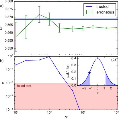
Figure 2: Scalar two-sample test for the Binder cumulant $U_{4}$ in the Ising model obtained from Markov chain Monte Carlo with Wolff cluster updates at temperature $T=2.3$ for system length $L=32$. (a) Sample mean of $U_{4}$ of an erroneous implementation for different simulation times $N$, and the result of a correct reference simulation; (b) corresponding $p$ values computed using Eq. (6); (c) illustration of the $p$ value for $N^{\prime}=10^{3}$ ($N=123$ after the removal of autocorrelation and variance pooling) as the shaded area under the probability density function (p.d.f.) of the corresponding $t$ distribution.

As an example, we reexamine data from the Ising model, this time on a $32\times 32$ square lattice. We verify the estimator for the Binder cumulant Binder (1981)

$$\hat{U}_{4}=\frac{\langle m^{4}\rangle}{1-3\langle m^{2}\rangle^{2}}.$$ (8)

The Student $t^{2}$ test is sensitive to non-Gaussian distributed errors, which occur in the computation of Eq. (8) due to non-linear error propagation. To remedy this, we use the jackknife resampling procedure, which replaces Eq. (8) with a simple average $\langle U_{4}^{\prime}\rangle$ over pseudovalues $U_{4}^{\prime}$, removing the linear order of the bias and restoring the validity of Eq. (6) Efron (1982). Alternatively, one could abandon the the Student test altogether in favor of the parametric bootstrap method Efron (1982). However, we will see that the jackknife method suffices in our case.

To simulate a common programming error, we have artificially broken periodic boundary conditions on the corners of the lattice (they are reduced to having two neighbors each). Fig. 2(a) compares this erroneous implementation (green curve) with a simulation result where the error is not present. As evident from Fig. 2(b), as we increase the number of Monte Carlo sweeps $N^{\prime}$, the error bars shrink and the null hypothesis (5a) is rejected more and more strongly.

III Data series tests

III.1 Tests for the mean

While tests for scalar quantities (Sec. II) are useful, we empirically find that it is often easier to identify problems when comparing functions and data series. In the case of a one-sample test, this corresponds to the benchmark result $y$ being a vector of $n$ elements rather than a scalar. Consequently, the Monte Carlo estimator $\hat{X}$ is vector-valued. Again assuming independent and identically distributed results, Eq. (2) is replaced by Hotelling (1931)

$$N(\langle X\rangle-x_{0})^{\mathrm{T}}\Sigma_{X}^{-1}(\langle X\rangle-x_{0})\sim\frac{n(N-1)}{N-n}F_{n,N-n}\;,$$ (9)

where $\langle X\rangle$ is the sample mean, $\Sigma_{X}$ is the sample covariance matrix, and $F_{a,b}$ is the Fisher–Snedecor distribution with parameters $a$, $b$. One proceeds in a similar way to the Student’s $t$-test. The observed left-hand side of Eq. (9) is again used as the test statistic and checked against the right-hand side distribution. However, since the $F$ distribution is not symmetric for low $n$ (cf. Fig. 3(c)), one uses two one-sided tests instead of a two-sided test and subsequently obtains two $p$-values, which we will call $p_{<}$ and $p_{>}$. This is known as Hotelling’s $T^{2}$ test.

In the case where we compare the estimator to a trusted result $\langle Y\rangle$, we proceed similar as in Sec. II.2 and replace Eq. (9) with:

$$\begin{split}&N_{\mu}(\langle X\rangle-\langle Y\rangle)^{\mathrm{T}}\Sigma^{-1}(\langle X\rangle-\langle Y\rangle)\\ &\qquad\sim\frac{n(N_{X}+N_{Y}-2)}{N_{X}+N_{Y}-n-1}F_{n,N_{X}+N_{Y}-n-1}\;,\end{split}$$ (10)

where $\Sigma$ is the pooled covariance obtained by replacing all variances $\sigma_{a}^{2}$ with covariance matrices $\Sigma_{a}$ in Eq. (7).

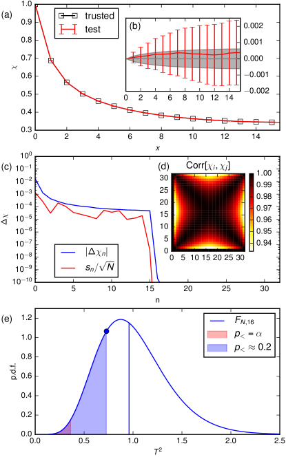
Figure 3: Vector-valued two-sample test on the spin correlation function $\chi_{x,0}$ (cf. Eq. (11)). (a) Simulation result for Wolff updates (black curve) and single spin-flip updates (red curve); (b) deviation of spin-flip from Wolff update (the shaded region are the Wolff result error bars); (c) Projected deviations and errors (numerator and denominator in the l.h.s. of Eq. (14)); (d) correlation matrix (12); (e) p.d.f. of the corresponding $F$ distribution in Eq. (14) with the mean as vertical blue line and $p_{<}$-value as blue shaded area to the left of the observed $T^{2}$ score (blue dot) as well as test failure threshold as red-shaded area.

In order to illustrate the procedure, we revisit our Ising model example for $L=32$ and $T=2.3$ (close to the critical temperature) and examine the spin correlation function

$$\begin{split}\chi_{x,y}&=\langle\sigma_{0,0}\sigma_{x,y}\rangle\\ &=\frac{1}{L^{2}}\langle\sum_{k,q}\sum_{x^{\prime},y^{\prime}}\mathcal{F}_{x,y;k,q}^{-1}|\mathcal{F}_{k,q;x^{\prime},y^{\prime}}\sigma_{x^{\prime},y^{\prime}}|^{2}\rangle,\end{split}$$ (11)

where $(x,y)$ denote row and column of the lattice site, and $\mathcal{F}$ denotes the discrete Fourier transform used in the actual estimator. Fig. 3(a) shows $\chi_{x0}$ for the Wolff cluster update (black curve), which we take as the trusted result, and for a set of spin-flip updates (red curve). The inset Fig. 3(b) shows the deviation of the red curve from the black one, where the shaded region marks the error bars of the Wolff update result. We see significant correlation of the error bars, which underscores the importance of a proper treatment of the covariance matrix (cf. Fig. 3(d)).

III.2 Cross-correlated data

A common complication with the $T^{2}$ test are perfect correlation or anti-correlation within the dataset (duplicates), which implies a singular covariance matrix in Eq. (9). In our example, the symmetry of the system implies $\chi_{x,y}=x_{L-x,y}$, thus half of the points yielded by the estimator (11) are just copies of the other half. We can confirm this by examining the correlation matrix:

$$\mathrm{Corr}[\chi_{x,0},\chi_{x^{\prime},0}]=\frac{\mathrm{Cov}[\chi_{x,0},\chi_{x^{\prime},0}]}{\sqrt{\mathrm{Var}[\chi_{x,0}]\mathrm{Var}[\chi_{x^{\prime},0}]}},$$ (12)

plotted in Fig. 3(d), which is one on the anti-diagonal.

This can be solved by first diagonalizing $\Sigma$ and retaining only the non-zero eigenvalues (a relative threshold of $10^{-14}$ seems to be practical for most cases we studied):

$$\Sigma=\mathcal{P}\;\mathrm{diag}(s_{1}^{2},\ldots,s_{m}^{2})\;\mathcal{P}^{\mathrm{T}},$$ (13)

where $\mathcal{P}$ is the $n\times m$ projection to the non-zero eigenvalues $s_{1}^{2},\ldots,s_{m}^{2}$. This is shown in Fig. 3(c), where there is sharp drop of $s_{n}$ (red curve) in magnitude after $m=15$. Eq. (9) is then amended to:

$$\sum_{i=1}^{m}\frac{|\sum_{k=1}^{n}\mathcal{P}_{ki}(\langle X_{k}\rangle-y_{k})|^{2}}{s_{i}^{2}/N}\sim\frac{m(N-1)}{N-m}F_{m,N-m}.$$ (14)

Note the reduction in the degrees of freedom from $n$ to $m$, which corresponds to discarding the $n-m$ correlated data points. Note also that for $n=m$ Eq. (9) and Eq. (14) are equivalent, such that in practical calculations, one can always use Eq. (14). Finally, we perform a $T^{2}$ test against the appropriate $F$ distribution and find that the null hypothesis is accepted with $p\approx 0.2$ (Fig. 3(e)).

III.3 Error bars

By using the sample mean and covariance as input rather than the individual samples, one can interpret Hotelling’s $t^{2}$ test as statistical test on the error bars $\sigma_{0}$ :

$$H_{0} :\sigma=\sigma_{0}$$ (15a)

$$H_{1}^{-} :\sigma<\sigma_{0}$$ (15b)

$$H_{1}^{+} :\sigma>\sigma_{0}$$ (15c)

For a scalar estimator (Sec. II), we can distinguish $H_{0}$ from $H_{1}^{-}$: error bars being “too small” (15b) is equivalent to the result being inconsistent with the benchmark (Eq. (1b)). However, we cannot test against $H_{1}^{+}$, since we may have accidentally hit the benchmark accurately. Using a data series, we can also distinguish it from $H_{1}^{+}$, formalizing the rule that “roughly two-thirds of the data should fall within one-sigma error-bars”. This is reflected in the fact that for $n>1$, the $F$ distribution turns from a one-tailed to a two-tailed distribution, and becomes more symmetric around $1$ as $n$ gets larger. We can make use of this by testing the lower tail as score for $H_{1}^{+}$ and the upper tail as score for $H_{1}^{-}$.

This procedure is illustrated at the example of the estimator for $\chi_{i,0}$ (Sec. III). If we ignore the cross-correlation (Fig. 3d) and interpret the error bars in Fig. 3b as uncorrelated errors, it is evident from visual inspection that they are too large. We can confirm this numerically by (erroneously) plugging the diagonal elements $\Sigma_{ii}$ of the covariance matrix instead of its eigenvalues $s_{i}$ into Eq. (14). We then find a $T^{2}$ score of $0.03$ and an acceptance of the lower alternate hypothesis $H_{1}^{+}$ (15b) with $p=1-10^{-16}$.

IV Example: Anderson impurity model

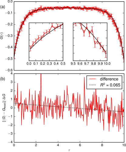
Figure 4: (a) Green’s function $G(\tau)$ for AIM parameters as in main text: Monte Carlo result (red) and exact result with an artificially introduced shift of the half bin size, i.e., $G(\tau-0.02)$, (black) modeling a binning error; (b) deviation from the exact result in multiples of the standard error as well as a linear regression (black dashed line) $0.539-0.098\tau$ with a goodness of fit of $R^{2}\approx 0.065$.

To illustrate our method on a research example, we examine the single-orbital Anderson impurity model Anderson (1961) (AIM) which characterizes a few discrete and potentially correlated impurity states coupled to a non-interacting bath. The model is in wide use in nano- and transport science Hanson et al. (2007); Brako and Newns (1981) and as an auxiliary model in the dynamical mean field theory Georges et al. (1996), and in many parameter regimes quantum Monte Carlo methods are the standard tools for obtaining its properties Gull et al. (2011). Its Hamiltonian is

$$\begin{split}\mathcal{H}=&\;Uc_{\uparrow}^{\dagger}c_{\downarrow}^{\dagger}c_{\downarrow}c_{\uparrow}-\mu\sum_{\sigma}c_{\sigma}^{\dagger}c_{\sigma}\\ &+\sum_{p\sigma}(V_{p\sigma}f_{p\sigma}^{\dagger}c_{\sigma}+\mathrm{h.c.})+\sum_{p\sigma}\epsilon_{p}f_{p\sigma}^{\dagger}f_{p\sigma}.\end{split}$$ (16)

Here, $c_{\sigma}$ annihilates a fermion of spin-$\sigma$ on the impurity and $f_{p\sigma}$ annihilates a bath fermion of momentum $p$ and spin $\sigma$. Impurity interactions are characterized by $U,$ $\mu$ denotes a chemical potential, $V$ a spin- and momentum dependent hybridization term, and $\epsilon_{p}$ a momentum-dependent bath dispersion. In the context of the AIM, a truncation of the bath to a few states and subsequent exact diagonalization of the finite system is particularly suitable for testing. While the complexity of solving the model with Monte Carlo methods is the same as for a model without bath truncation, one empirically finds that the truncated model shares much of the physics of the AIM and can thus be used to generate non-trivial, analytically accessible test cases for Monte Carlo simulations.

Our example consists of two momenta and correspondingly two bath sites with energies of $\epsilon_{p}=\pm 0.5$ and a hybridization strength $V=1$, as well as $U=5$, $\mu=U/2$, and temperature $T=1/10$. Stochastic results were obtained using continuous-time quantum Monte Carlo in the hybridization expansion Werner and Millis (2006); Gull et al. (2011).

The imaginary time Green’s function $G(\tau)=-\langle Tc(\tau)c^{\dagger}(0)\rangle,$ which is the fundamental quantity of interest in this model and which is directly related to the interacting spectral function, is shown in Fig. 4. In order to mimic the effect of a typical binning programming error, we have shifted the exact result (black) by half a bin $G(\tau)\to G(\tau-0.02)$. The top panel shows that the Monte Carlo result (red) is still consistent with the exact result in this case when gauged by visual inspection. This is reinforced by the bottom panel, where the deviation from the exact result in multiples of the standard error is plotted (red). Overall we find the expected result, even though a linear fit of the data (shown as black dashed line) shows a slight downward slope indicative of a problem.

However, Hotelling’s $T^{2}$ test finds a test statistic of $T^{2}\approx 1.28$ and therefore a rejection of the null hypothesis in favor of $H_{1}^{+}$ with $p\approx 0.0026$ (about three sigma). This is because by using all $n=250$ data points, the test becomes sensitive to a small increase of the values outside of error bars. Systematically increasing the statistics would eventually expose the deviation to visual inspection.

V Conclusions

In this paper, we have shown how hypothesis testing can be used to develop tests for code correctness of Monte Carlo codes in statistical and condensed matter physics. We also have shown how these tests are sensitive to different types of simulation problems, and how they can therefore be used as diagnostic tools to ensure the correctness of simulations.

The mathematical framework for hypothesis testing has been known for over 100 years and statistical tests are in wide use across many scientific fields. Despite this, the technique is not used on a routine basis for testing scientific simulation results. With the advent of automatic testing and unit test frameworks, which have permeated most of software engineering and to some extent also scientific computing, our techniques add to the testing toolkits that can be used to systematically ensure correctness and reproducibility of stochastic physics simulations. These tests integrate well into existing testing frameworks and can validate parts of the programs that are otherwise difficult to test.

Hypothesis testing allows to gain and keep trust in complex codes as they undergo modifications, and to uncover problems that are difficult to uncover by other means, e.g. manual visual inspection. This both increases the speed of scientific software development and the trust in results produced by complex computer programs.

In our opinion hypothesis testing should be widely adopted in statistical simulation codes and should become a standard tool in scientific software development. While implementing these tests carries a small overhead, we argue that rigorous, frequent, and automatic testing is necessary for today’s codes, especially in light of the replication crisis Baker (2016) observed in other fields of science.

The code for the stochastic solvers and the hypothesis testing post-processing scripts are available from the authors upon request. An open-source software implementation of hypothesis testing is scheduled for inclusion in the upcoming version of the ALPS core libraries.Gaenko et al. (2017)