Planar screening by charge polydisperse counterions

Abstract

We study how a neutralising cloud of counterions screens the electric field of a uniformly charged planar membrane (plate), when the counterions are characterised by a distribution of charges (or valence), $n(q)$. We work out analytically the one-plate and two-plate cases, at the level of non-linear Poisson-Boltzmann theory. The (essentially asymptotic) predictions are successfully compared to numerical solutions of the full Poisson-Boltzmann theory, but also to Monte Carlo simulations. The counterions with smallest valence control the long-distance features of interactions, and may qualitatively change the results pertaining to the classic monodisperse case where all counterions have the same charge. Emphasis is put on continuous distributions $n(q)$, for which new power-laws can be evidenced, be it for the ionic density or the pressure, in the one- and two-plates situations respectively. We show that for discrete distributions, more relevant for experiments, these scaling laws persist in an intermediate but yet observable range. Furthermore, it appears that from a practical point of view, hallmarks of the continuous $n(q)$ behaviour is already featured by discrete mixtures with a relatively small number of constituents.

I Introduction

Polydispersity refers to non-uniformity in some property. For soft matter, it can pertain to size, surface features, charges, electrolytic content etc., and lead to baffling complexity in structural or dynamical properties ILMR ; TaAr95 . Not only can some structures be destabilised vdLBD13 , nucleation AuFr01 or compressibility BCCD11 be suppressed, but also fractionation may ensue Bart00 ; SoWi11 or super-lattices appear ElMF93 ; BCGJ16 . In the limit of a continuous mixture of hard sphere, it was shown that optimal packing yields the formation of macroscopic aggregates, in a scenario that bears similarities with Bose-Einstein condensation ZBTC99 ; BlCu01 .

The present paper is devoted to charged fluids, and to the physics of screening by a polydisperse ensemble of counterions, having different valence. There is a number of reasons for investigating such problems. First of all, multivalent ions of distinct charges are routinely found in a wealth of situations. One may think here of spermine and spermidine ions in biological systems AnRe80 . Also, the upsurge of interest for nanocolloidal systems provides a motivation for our work, where the presence of distinct species with specific charges should be accounted for exp1 ; exp2 . A specific feature of a linear description, à la Debye and Hückel Levin02 , of the kind of polydispersity we are interested in, is entirely subsumed into the so-called Debye length, which is a very coarse measure of the dispersion in ionic valences. Yet, non-linear effects, overlooked at the Debye-Hückel level, deeply affect the structure of the electric double-layer in the vicinity of charged macromolecules UhGK01 ; TeTr04 ; TrTe06 : the sole Debye length is not sufficient to characterise screening, and thus interactions between charged bodies. Our analysis is worked out at the level of the non-linear Poisson-Boltzmann theory, where it is interesting to note that the problem of mixed valences has been investigated in the pioneering paper of Gouy Gouy10 . Yet, exact results are scarce, even in the planar geometry to which we restrict our study. To complement the analytical derivation, Monte Carlo simulation results will also be reported.

To magnify non-linear effects, we will be interested in a counterion only system (the limit of a completely deionised solution deionised ), and analyse screening of planar charged bodies. A number of new analytical results can then be derived. In this very geometry, parallel like-charged plates interact at long-distances in a universal fashion, provided only one type of counterion is present in the solution (mono-disperse case). It can indeed be readily shown that the corresponding pressure behaves like $P\sim\pi kT/(2\ell_{\rm B}d^{2})$ where $d$ is the inter-plate distance, and $\ell_{\rm B}$ is the Bjerrum length defined below, scaling like the elementary charge squared Andelman06 . Thus, the previous large-$d$ result is universal, independent of the charge on the plates. This result can be generalised to any polydisperse counterionic mixture, under the proviso that there is a lower bound $q_{\text{min}}>0$ in the valence distribution. Here, the ions with smaller valence are less attracted to the charged plates, and are those mediating the interaction force. Those ions with valence larger than $q_{\text{min}}$ screen the plates’ bare charge, reducing its effective value, which however does not enter the large-$d$ behaviour. We thus expect the universal asymptotic $P\propto q_{\text{min}}^{-2}d^{-2}$ to be valid as well for a mixture, be it discrete or continuous, as long as $q_{\text{min}}>0$. We will see in particular that whenever $q_{\text{min}}=0$, the situation changes completely, and that new power-law regimes emerge, with a $d$-exponent smaller than 2 that can be tuned continuously. This is a consequence of less efficient screening, resulting in a severe enhancement of effective interactions. In a sense to be specified though, these interactions keep some level of universality.

The paper is organized as follows. We present in Sections II and III the results for the one-plate and two-plates geometries. These are tested against numerical simulations, of two distinct types: numerical resolution of Poisson-Boltzmann theory on the one hand, and Monte Carlo simulations on the other hand. The numerical techniques used are sketched in the appendix. Finally, our main results are recovered and extended in a heuristic and rather direct way in section IV. A significant part of the analytical treatment (with the notable exception of the statements that do not pertain to asymptotic results) is devoted not only to continuous distributions $n(q)$, but furthermore, to distributions having a vanishing minimum charge $q_{\text{m}in}$. The reason is that the behaviour of $n(q)$ for $q\to 0$ is at the root of new scaling laws for the long-distance ionic profiles, or interplate pressures. Indeed, those counterions with a large valency will be more attracted to the charged plates, while the others are less localised, and play a more important role in large scale features. Yet, the corresponding “continuous models” might be viewed as somewhat artificial, since any physical system exhibiting polydispersity in counterion charge will have $q_{\text{m}in}>0$. In section IV, we shall address that legitimate concern, and show that the newly found power-laws can be observed over an intermediate range if $q_{\text{m}in}>0$ or in discrete systems. In addition, we will present numerical data illustrating the fact that in some cases, a small number of species is sufficient for a system to exhibit the continuous polydispersity asymptotics. Some attention will also be paid to universal features that may characterize density profiles and equations of state.

II One-wall geometry

We consider a hard wall of dielectric constant $\epsilon^{\prime}$ localised in the half-space $x<0$. The Cartesian $(y,z)$ coordinates are unbounded. The surface of the wall at $x=0$ carries a constant surface charge density $\sigma e$ ($e$ is a unit charge and say $\sigma>0$). Mobile particles, confined in the half-space $x>0$, are immersed in a medium of dielectric constant $\epsilon$. We assume for simplicity that $\epsilon^{\prime}=\epsilon$, i.e. there are no electrostatic image charges. Particles can have various charges, with sign opposite to that of the plate: they are counterions. Let $\rho(x)$ be the particle charge density (per unit surface of the wall) at distance $x$ from the wall. The condition of overall electroneutrality reads

$$\sigma e+\int_{0}^{\infty}{\rm d}x\,\rho(x)=0.$$ (1)

The mean electrostatic potential $\psi(x)$ fulfils the Poisson equation

$$\frac{{\rm d}^{2}\psi(x)}{{\rm d}x^{2}}=-\frac{4\pi}{\epsilon}\rho(x).$$ (2)

Integrating this equation over $x$ from $0$ to $\infty$, the requirement of electroneutrality (1) is consistent with the couple of boundary conditions (BCs)

$$\psi^{\prime}(0)=-\frac{4\pi\sigma e}{\epsilon},\qquad\psi^{\prime}(\infty)=0.$$ (3)

II.1 Monodisperse case

We first recapitulate briefly the monodisperse results Andelman06 where all mobile ions possess the same charge, say $-e<0$ (i.e. their valence is $q=1$). Denoting by $n(x)$ the particle number density at $x$, the charge density is simply $\rho(x)=-en(x)$.

The statistical mechanics of the system is described by the mean-field Poisson-Boltzmann (PB) theory Gouy10 ; Chapman13 , provided Coulombic coupling is small enough NJMN05 ; SaTr11 ; Rque03 . In the PB approach, the density of particles at a given point is proportional to the corresponding Boltzmann weight of the mean electrostatic potential,

$$n(x)=f_{0}\,{\rm e}^{\beta e\psi(x)},$$ (4)

where $f_{0}$ is a normalisation constant and $\beta$ denotes the inverse temperature. Introducing the reduced potential

$$\phi(x)=\beta e\psi(x),\qquad n(x)=f_{0}\,{\rm e}^{\phi(x)},$$ (5)

this mean-field assumption applied to (2) leads to the PB equation

$$\frac{{\rm d}^{2}\phi(x)}{{\rm d}x^{2}}=4\pi\ell_{\rm B}f_{0}\,{\rm e}^{\phi(x)},$$ (6)

where $\ell_{\rm B}\equiv\beta e^{2}/\epsilon$ is the Bjerrum length. Note that the shift of $\phi$ by a constant only renormalizes $f_{0}$. We fix the potential gauge by setting

$$\phi(0)=0$$ (7)

at the wall. Once a gauge has been chosen, $f_{0}$ is directly related to the contact density of counterions, $n(0)$. The BCs (3) read for the reduced potential as follows

$$\phi^{\prime}(0)=-4\pi\ell_{\rm B}\sigma,\qquad\phi^{\prime}(\infty)=0.$$ (8)

Since $\phi^{\prime}(x)\leq 0$ and with regard to the gauge (7), it holds that $\phi(x)\leq 0$. Due to the absence of the neutralising bulk background (like in jellium models), the bulk particle density vanishes and so $\phi(x)$ goes to $-\infty$ at asymptotically large $x$. This is the reason why an approach à la Debye-Hückel necessarily fails here, since it relies on linearising the problem around a point of reference, taken usually for a one macroion problem as the bulk surrounding electrolyte. Here, we have no electrolyte, only counterions.

Multiplying the PB equation (6) by $\phi^{\prime}(x)$, it can be rewritten as Andelman06

$$\frac{1}{2}\frac{{\rm d}}{{\rm d}x}\left[\phi^{\prime}(x)\right]^{2}=4\pi\ell_{\rm B}f_{0}\,\frac{{\rm d}}{{\rm d}x}{\rm e}^{\phi(x)},\qquad\frac{1}{2}\left[\phi^{\prime}(x)\right]^{2}=4\pi\ell_{\rm B}f_{0}\,{\rm e}^{\phi(x)},$$ (9)

where the integration constant equals to 0 due to the BCs $\phi^{\prime}(x)\to 0$ and ${\rm e}^{\phi(x)}\to 0$ in the limit $x\to\infty$. The gauge (7) and the first BC in (8), when considered in (9), fix the normalization constant to $f_{0}=2\pi\ell_{\rm B}\sigma^{2}$. The resulting first-order differential equation

$$\phi^{\prime}(x)=-4\pi\ell_{\rm B}\sigma{\rm e}^{\phi(x)/2}$$ (10)

with the BC $\phi(0)=0$ is solvable by the method of the separation of variables:

$$\phi(x)=-2\ln\left(1+\widetilde{x}\right),$$ (11)

where $\widetilde{x}$ is the dimensionless distance given by

$$\widetilde{x}\equiv\frac{x}{\mu},\qquad\mu=\frac{1}{2\pi\ell_{\rm B}\sigma}$$ (12)

$\mu$ being the Gouy-Chapman length. The electric potential goes to $-\infty$ at asymptotically large distances from the wall logarithmically. The particle number density behaves as

$$n(x)=f_{0}\,{\rm e}^{\phi(x)}=2\pi\ell_{\rm B}\sigma^{2}\frac{1}{(1+\widetilde{x})^{2}}\mathop{\sim}_{x\to\infty}\frac{1}{2\pi\ell_{\rm B}}\frac{1}{x^{2}}.$$ (13)

The value of the number density at $x=0$, $n(0)=2\pi\ell_{\rm B}\sigma^{2}$, is in agreement with the contact theorem Henderson78 ; Henderson79 ; Choquard80 ; Carnie81 ; Totsuji81 ; Wennerstrom82 ; Mallarino15 . We further see that the large-distance decay of the particle number density is universal, independent of the surface charge density $\sigma e$: the only restriction is that $\sigma\neq 0$. This well known but remarkable result illustrates in a particular strong form a phenomenon of saturation, considered as a hallmark of Poisson-Boltzmann theory: upon increasing the charge of a field-creating macroion, one eventually reaches a regime where the electrostatic signature becomes independent of the macroion charge BoTA02 ; TeTr03 . Here, not only is saturation observed at finite $x$ increasing $\sigma$ (and thus letting $\mu\to 0$), but it is also met – and this is specific to one dimensional geometry – at any finite $\sigma$ for $x\to\infty$. In both cases, this is a signature of efficient screening. We will see below that these properties are lost for certain classes of polydisperse counterionic systems, where screening is impeded by counterions of a too small valence.

II.2 Polydisperse case

We now consider counterions with charges $-qe$, where $q$ is constrained to the interval $[0,1]$. The upper bound is arbitrary and rather than some $q_{\text{max}}$, we take it to be unity for the sake of convenience. We stress here that when results are rescaled with the mean value $\langle q\rangle$, they become independent of the choice of $q_{\text{max}}$. The model is defined by a density distribution (per unit surface) $n(q)$ of particles with the charge $-qe$. The distribution $n(q)$ might be discrete, i.e. it is a sum of $\delta$-functions, or continuous; for the next treatment, we consider that $n(q)$ is continuous at least close to $q=0$. We define the (normalised) moments of the $n(q)$-distribution as follows

$$\langle q^{j}\rangle\equiv\frac{\int_{0}^{1}{\rm d}q\,q^{j}n(q)}{\int_{0}^{1}{\rm d}q\,n(q)},\qquad j=1,2,\ldots.$$ (14)

Within the PB theory, the density of particles with charge $q$ at distance $x$ from the wall, $n(q,x)$, is expressed as

$$n(q,x)\,=\,f(q)\,{\rm e}^{q\phi(x)},$$ (15)

where $f(q)$ is a positive normalisation function; it was equal to $f_{0}\,\delta(q-1)$ in the monodisperse system. From this relation, the total particle number density at $x$ is given by

$$n(x)=\int_{0}^{1}{\rm d}q\,n(q,x)=\int_{0}^{1}{\rm d}q\,f(q){\rm e}^{q\phi(x)}.$$ (16)

The charge density at $x$ is expressible as

$$\rho(x)=\int_{0}^{1}{\rm d}q\,(-eq)n(q,x)\,=\,-e\,\int_{0}^{1}{\rm d}q\,qf(q){\rm e}^{q\phi(x)}=-e\,\frac{n^{\prime}(x)}{\phi^{\prime}(x)}.$$ (17)

The number density distribution $n(q)$ is given by

$$n(q)=\int_{0}^{\infty}{\rm d}x\,n(q,x)=f(q)\int_{0}^{\infty}{\rm d}x\,{\rm e}^{q\phi(x)}.$$ (18)

This equation relates the density distribution $n(q)$ and the normalisation function $f(q)$, provided that the reduced potential $\phi(x)$ is known. The overall electroneutrality of the system leads to a constraint for $n(q)$:

$$\sigma\,=\,\int_{0}^{\infty}{\rm d}x\,\frac{\rho(x)}{-e}\,=\,\int_{0}^{1}{\rm d}q\,q\,n(q).$$ (19)

Here, it is worth pointing to a subtlety, that lies in the difference between $f(q)$ and $n(q)$. In a “particle” based model, such as a Monte Carlo simulation, one chooses the identity of the counterion, thereby fixing the function $n(q)$. Then, $f(q)$ follows in a non-trivial way, from measuring the equilibrium density profiles of $q$-species. On the other hand, in a “field” based formulation such as PB theory, one needs to know $f(q)$ to be able to write the differential equation to be solved. Starting from $n(q)$, this requires the knowledge of the potential $\phi(x)$, which is precisely the object we are looking for. This difficulty is essentially absent in the monodisperse case; it is the main complication to be addressed when considering polydisperse mixtures.

Inserting $\rho(x)$ (17) into the Poisson equation, we get the polydisperse PB equation

$$\frac{{\rm d}^{2}\phi(x)}{{\rm d}x^{2}}\,=\,4\pi\ell_{\rm B}\,\int_{0}^{1}{\rm d}q\,q\,f(q)\,{\rm e}^{q\phi(x)}.$$ (20)

The gauge (7) and the BCs (8) remain unchanged, i.e.

$$\phi(0)=0,\qquad\phi^{\prime}(0)=-4\pi\ell_{\rm B}\sigma,\qquad\phi^{\prime}(\infty)=0.$$ (21)

As before, $\phi(x)$ goes to $-\infty$ at asymptotically large $x$. The problem of the polydisperse PB formulation, alluded to above, is that the available information about the charge mixture is encoded in the density distribution of the charged particle $n(q)$, and not in the normalisation function $f(q)$. But the natural (or at least analytically convenient) formulation is in fact inverse: with a prescribed normalisation function $f(q)$, one should solve the PB equation (respecting the corresponding BCs) for the reduced potential and then obtain the density distribution $n(q)$ of the charged particles by using the $n-f$ relation (18). We explain in the appendix how this complication was circumvented for numerical purposes. As far as analytical results are concerned, the “implicit” formulation of Eq. (20) is not an issue.

As in the monodisperse case, the PB equation (20) can be integrated into

$$\left[\phi^{\prime}(x)\right]^{2}=8\pi\ell_{\rm B}\int_{0}^{1}{\rm d}q\,f(q){\rm e}^{q\phi(x)}.$$ (22)

The integration constant is again equal to $0$ due to the BCs $\phi^{\prime}(x)\to 0$ and ${\rm e}^{\phi(x)}\to 0$ in the limit $x\to\infty$. The gauge and the BC at $x=0$ imply the constraint

$$\int_{0}^{1}{\rm d}q\,f(q)=2\pi\ell_{\rm B}\sigma^{2},$$ (23)

which is equivalent to the fact that, according to the contact theorem Henderson78 ; Henderson79 ; Choquard80 ; Carnie81 ; Totsuji81 ; Wennerstrom82 ; Mallarino15 , the contact density $n(0)=2\pi\ell_{\rm B}\sigma^{2}$. Equation (22) can be rewritten as follows

$$\left[\phi^{\prime}(x)\right]^{2} = 8\pi\ell_{\rm B}\int_{0}^{1}{\rm d}q\,f(q){\rm e}^{-q[-\phi(x)]}$$ (24)

$$= 8\pi\ell_{\rm B}\int_{0}^{-\phi(x)}\frac{{\rm d}p}{[-\phi(x)]}f\left(\frac{p}{-\phi(x)}\right){\rm e}^{-p}.$$

In the polydisperse case, we define the dimensionless distance as

$$\widetilde{x}\equiv\frac{x}{\mu},\qquad\mu=\frac{1}{2\pi\ell_{\rm B}\sigma\langle q\rangle}.$$ (25)

Note that this definition is consistent with that used in the monodisperse case (12) for which $\langle q\rangle=1$. We know that in the limit $x\to\infty$ the function $-\phi(x)\to\infty$. This means that at asymptotically large distances only the leading small-$q$ term of the positive distribution function $f(q)$ matters in Eq. (24). It is also clear that $f(q)\to 0$ for $q\to 0$. From Eq. (18) indeed, this is the only way to ensure a non-divergent surface density $n(q)$ for $q\to 0$. Let us then suppose that

$$f(q)\mathop{\sim}_{q\to 0}2\pi\ell_{\rm B}\sigma^{2}a\,q^{\alpha},$$ (26)

where $a>0$ and $\alpha\geq 0$ are some dimensionless parameters; the presence of the prefactor $2\pi\ell_{\rm B}\sigma^{2}$ is motivated by the constraint (23). Considering this small-$q$ behaviour, we show in Appendix A that it is possible to work out the long-distance asymptotic for all quantities of interest (charge density, ionic density, electrostatic potential), where novel scaling laws – explicitly dependent on exponent $\alpha$ – do emerge.

A meaningful way to present the results is to introduce $\gamma=(\alpha-3)/2$, which turns out to characterise the small-$q$ behaviour of the charge distribution:

$$\frac{n(q)}{\sigma}\mathop{\sim}_{q\to 0}cq^{\gamma},$$ (27)

which defines the parameters $c>0$ and $\gamma>-1$. The results derived in Appendix A then translate into

$$\phi(\widetilde{x})\mathop{\sim}_{\widetilde{x}\to\infty}-\left[c\frac{2^{2\gamma+5}}{\sqrt{\pi}}\frac{\gamma+3}{\gamma+2}\Gamma\left(\gamma+\frac{5}{2}\right)\right]^{\frac{1}{\gamma+3}}(\widetilde{x}/\langle q\rangle)^{\frac{1}{\gamma+3}},$$ (28)

$$n(\widetilde{x})\mathop{\sim}_{\widetilde{x}\to\infty} 2\pi\ell_{\rm B}\sigma^{2}\left[c\frac{2^{\gamma+2}}{\sqrt{\pi}}\frac{1}{(\gamma+2)(\gamma+3)^{\gamma+2}}\Gamma\left(\gamma+\frac{5}{2}\right)\right]^{\frac{2}{\gamma+3}}\frac{1}{(\widetilde{x}/\langle q\rangle)^{2\left(\frac{\gamma+2}{\gamma+3}\right)}},$$ (29)

$$\frac{\rho(\widetilde{x})}{(-e)}\mathop{\sim}_{\widetilde{x}\to\infty}2\pi\ell_{\rm B}\sigma^{2}\left[c\frac{2^{\gamma+2}}{\sqrt{\pi}}\frac{(\gamma+2)^{\gamma+2}}{(\gamma+3)^{2\gamma+5}}\Gamma\left(\gamma+\frac{5}{2}\right)\right]^{\frac{1}{\gamma+3}}\frac{1}{(\widetilde{x}/\langle q\rangle)^{\frac{2\gamma+5}{\gamma+3}}}.$$ (30)

In particular, when $n(q)$ goes to a nonzero constant $c$ in the limit $q\to 0$, which corresponds to $\gamma=0$, we have

$$\phi(\widetilde{x})\mathop{\sim}_{\widetilde{x}\to\infty}-6^{2/3}c^{1/3}(\widetilde{x}/\langle q\rangle)^{1/3},\quad n(\widetilde{x})\mathop{\sim}_{\widetilde{x}\to\infty}2\pi\ell_{\rm B}\sigma^{2}\frac{1}{6^{2/3}}c^{2/3}\frac{1}{(\widetilde{x}/\langle q\rangle)^{4/3}},$$

$$\frac{\rho(\widetilde{x})}{(-e)}\mathop{\sim}_{\widetilde{x}\to\infty}2\pi\ell_{\rm B}\sigma^{2}\left(\frac{2}{9}\right)^{2/3}c^{1/3}\frac{1}{(\widetilde{x}/\langle q\rangle)^{5/3}}.$$ (31)

As we have seen, the non-universal large-distance behaviour of the quantities like the reduced potential and particle/charge densities for the charge mixtures within the PB theory can be related to the small-$q$ behaviour of the density distribution $n(q)$. If there is e.g. a gap in $q$ and the function $f(q)$, or equivalently $n(q)$, is zero up to some positive threshold $q_{\min}$, the integral in (22) is dominated by $\exp[q_{\min}\phi(x)]$ at large distances from the wall, and we basically recover the monodisperse relation of type (9). It is always the population with smallest valence which sets the large distance asymptotic, and non-trivial effects emerge when this population has a vanishing charge ($q_{\text{min}}=0$). A similar remark holds for the two-plate problem to be discussed below. Yet, even a discrete charge distribution may exhibit, transiently, the power-laws brought to the fore here, see section IV.3 below.

II.3 Numerical PB results for a simple polydisperse model

As emphasised above, a physical problem is posed specifying the distribution $n(q)$, rather than the normalisation function $f(q)$, which is unknown without having solved the PB equation, the formulation of which requires the knowledge of $f(q)$. This question will be addressed in the remainder (see the appendix), but to circumvent this complication and test the premises of our analytical approach, we have chosen the specific form

$$f(q)=2\pi\ell_{\rm B}\sigma^{2}aq^{\alpha}\qquad q\in[0,1],$$ (32)

with integer $\alpha=2,3,4,\ldots$. This function represents an extension of the small-$q$ asymptotic (26) to the whole $q$-interval. The constraint (23) fixes the prefactor $a$ to

$$a=\alpha+1.$$ (33)

The PB equation reads as

$$\phi^{\prime}(\widetilde{x})\langle q\rangle=-2\sqrt{\alpha+1}\left[\int_{0}^{1}{\rm d}q\,q^{\alpha}{\rm e}^{q\phi(\tilde{x})}\right]^{1/2}.$$ (34)

The advantage of the chosen model is that the function inside the integral on the rhs is explicitly integrable:

$$\int_{0}^{1}{\rm d}q\,q^{\alpha}{\rm e}^{q\phi} = \frac{{\rm e}^{\phi}(\phi^{2}-2\phi+2)-2}{\phi^{3}}\qquad\mbox{for $\alpha=2$,}$$ (35)

$$= \frac{{\rm e}^{\phi}(\phi^{3}-3\phi^{2}+6\phi-6)+6}{\phi^{4}}\qquad\mbox{for $\alpha=3$,}$$

$$= \frac{{\rm e}^{\phi}(\phi^{4}-4\phi^{3}+12\phi^{2}-24\phi+24)-24}{\phi^{5}}\qquad\mbox{for $\alpha=4$,}$$

etc. This allows us to solve numerically the PB equation in a particularly straightforward manner.

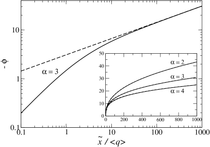
Figure 1: Log-log plot of the (minus) potential $-\phi$ vs. the reduced distance $\widetilde{x}/\langle q\rangle$ for $\alpha=3$. The solid curve corresponds to the numerical treatment of the PB equation with the normalisation function $f(q)$ defined by Eq. (32), the dashed line corresponds to the asymptotic formula (95). Inset: same results on a linear scale, for $\alpha=2,3$ and 4. The dashed and continuous lines are essentially superimposed.

For $\alpha=2,3,4$, the numerical results for the electric potential $\phi$ versus distance are presented by the solid curve in Fig. 1. For comparison, the analytically obtained asymptotic formula for the potential (95) are represented by the dashed lines. We see that the asymptotic regime is already reached at $\widetilde{x}/\langle q\rangle\sim 100$.

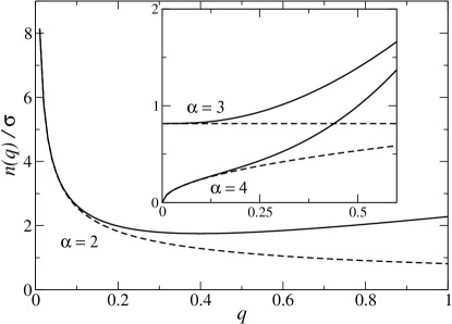
Figure 2: Plot of the particle density distribution $n(q)/\sigma$ vs. valence $q$ for $\alpha=2,3,4$. For each $\alpha$, the solid curve corresponds to the numerical solution of the PB equation with the normalisation function $f(q)$ defined by Eq. (32), while the dashed curve is for the asymptotic formula (101).

Having at our disposal the function $\phi(\widetilde{x})$, we calculate the particle density distribution $n(q)/\sigma$, which corresponds to our model (32), by using the formula (98). For $\alpha=2,3,4$, the numerical solution of the PB equation is represented by the solid curve in Fig. 2. The dashed curves appearing in this figure correspond to the asymptotic $q\to 0$ formula (101). As $q\to 0$, the density distribution diverges for $\alpha=2$, attains a finite value for $\alpha=3$ and goes to 0 for $\alpha=4$. We see that the agreement of the numerical and analytical calculations in the small-$q$ region is good. This confirms our previous assumption that the small-$q$ asymptotics of the functions $n(q)$ and $f(q)$ are related by Eq. (99) with the asymptotic large-$\widetilde{x}$ potential (95) inserted.

III Symmetric two-wall geometry

Now we consider a symmetric pair of parallel hard walls of dielectric constant $\epsilon$ at distance $d$. Each of the surfaces at $x=-d/2$ and $x=d/2$ carries a constant surface charge density $\sigma e$ with $\sigma>0$. The charged particles, confined to the slit $-d/2<x<d/2$, are immersed in a medium of the same dielectric constant as the walls, i.e. $\epsilon$. The electroneutrality condition reads as

$$2\sigma e+\int_{-d/2}^{d/2}{\rm d}x\,\rho(x)=0.$$ (36)

Integrating the Poisson equation (2) from $-d/2$ to $d/2$, the condition (36) is consistent with the couple of BCs

$$\psi^{\prime}\left(-\frac{d}{2}\right)=-\frac{4\pi\sigma e}{\epsilon},\qquad\psi^{\prime}\left(\frac{d}{2}\right)=\frac{4\pi\sigma e}{\epsilon}.$$ (37)

The problem is symmetric with respect to the sign reversal of the $x$-coordinate, i.e. $\psi(x)=\psi(-x)$, $n(x)=n(-x)$, $\rho(x)=\rho(-x)$. Consequently, $\psi^{\prime}(x)=-\psi^{\prime}(-x)$, $n^{\prime}(x)=-n^{\prime}(-x)$, $\rho^{\prime}(x)=-\rho^{\prime}(-x)$, so the derivatives of these quantities vanish at $x=0$. In particular,

$$\psi^{\prime}(0)=0.$$ (38)

This BC formally corresponds to having an uncharged hard wall at $x=0$.

For the subsequent analysis, it turns out that two equivalent formulations are of particular interest. They correspond to each other through a $x\to d/2-x$ transformation, with a additional shift of potential to enforce the chosen gauge.

• (i) In analogy with the one-plate problem, we shift the reference to the surface of one of the walls, say the one at $x=-d/2$, and consider the asymmetric configuration of one charged hard wall at $x=0$ with uniform surface charge density $\sigma e$, and one uncharged ($\sigma^{\prime}=0$) plain hard wall at $x=d/2$. The gauge condition and the corresponding BCs for the reduced potential read as

  $$\phi(0)=0,\qquad\phi^{\prime}(0)=-4\pi\ell_{\rm B}\sigma,\qquad\phi^{\prime}(d/2)=0.$$ (39)

  Both $\phi(x)$ and $\phi^{\prime}(x)$ are negative (or 0) in the whole interval $[0,d/2]$. In the monodisperse case, we set $n(x)=f_{0}\,{\rm e}^{\phi(x)}$ for the particle density and the resulting PB equation can be integrated into

  $$\left[\phi^{\prime}(x)\right]^{2}=8\pi\ell_{\rm B}f_{0}\,\left[{\rm e}^{\phi(x)}-1\right]+(4\pi\ell_{\rm B}\sigma)^{2}.$$ (40)

  Since the confining surfaces are planar, the particle densities at contact with the surfaces obey the contact theorem Henderson78 ; Henderson79 ; Choquard80 ; Carnie81 ; Totsuji81 ; Wennerstrom82 ; Mallarino15

  $$n(0)=2\pi\ell_{\rm B}\sigma^{2}+\beta P,\qquad n\left(\frac{d}{2}\right)=\beta P,$$ (41)

  where $P$ is the pressure. Equivalently,

  $$\beta P=f_{0}\,-2\pi\ell_{\rm B}\sigma^{2},\qquad\beta P=f_{0}\,{\rm e}^{\phi(d/2)}.$$ (42)

  In the polydisperse case with $n(x)=\int_{0}^{1}{\rm d}q\,f(q){\rm e}^{q\phi(x)}$, the PB equation can be integrated into

  $$\left[\phi^{\prime}(x)\right]^{2}=8\pi\ell_{\rm B}\int_{0}^{1}{\rm d}q\,f(q)\left[{\rm e}^{q\phi(x)}-1\right]+(4\pi\ell_{\rm B}\sigma)^{2}.$$ (43)

  The pressure can be written

  $$\beta P\,=\,\int_{0}^{1}{\rm d}q\,f(q)-2\pi\ell_{\rm B}\sigma^{2}\,=\,\int_{0}^{1}{\rm d}q\,f(q){\rm e}^{q\phi(d/2)}.$$ (44)

• (ii) Next, we shift the reference to the midpoint between the walls and consider the configuration of one uncharged ($\sigma^{\prime}=0$) hard wall at $x=0$ and the charged wall at $x=d/2$ with the (surface charge density $\sigma e$). The gauge condition and the corresponding BCs read as

  $$\phi(0)=0,\qquad\phi^{\prime}(0)=0,\qquad\phi^{\prime}(d/2)=4\pi\ell_{\rm B}\sigma.$$ (45)

  Both $\phi(x)$ and $\phi^{\prime}(x)$ are positive (or 0) in the interval $[0,d/2]$. In the monodisperse case, the PB equation is integrated into

  $$\left[\phi^{\prime}(x)\right]^{2}=8\pi\ell_{\rm B}f_{0}\,\left[{\rm e}^{\phi(x)}-1\right].$$ (46)

  The pressure is expressible as

  $$\beta P=f_{0}\,=\,f_{0}\,{\rm e}^{\phi(d/2)}-2\pi\ell_{\rm B}\sigma^{2}.$$ (47)

  On the other hand, the polydisperse PB equation can be integrated into

  $$\left[\phi^{\prime}(x)\right]^{2}=8\pi\ell_{\rm B}\int_{0}^{1}{\rm d}q\,f(q)\left[{\rm e}^{q\phi(x)}-1\right],$$ (48)

  and the pressure is given by

  $$\beta P=\int_{0}^{1}{\rm d}q\,f(q)\,=\,\int_{0}^{1}{\rm d}q\,f(q){\rm e}^{q\phi(d/2)}-2\pi\ell_{\rm B}\sigma^{2}.$$ (49)

Note that the explicit form of the normalisation function $f(q)$ depends on the formulation, while $\beta P$ does not.

III.1 Monodisperse case

In the monodisperse case with particles of charge $-e$, the solution is well known. For completeness, it is reminded here. We use formulation (ii) with the gauge and BCs of type (45). The PB equation (46), written as

$$\phi^{\prime}(x)=2K\sqrt{{\rm e}^{\phi(x)}-1},\qquad K=\sqrt{2\pi\ell_{\rm B}f_{0}},$$ (50)

has the explicit solution

$$\phi(x)=-2\ln\cos(Kx).$$ (51)

The BC at $x=d/2$ implies the transcendental equation for the screening parameter $K$:

$$Kd\tan\left(K\frac{d}{2}\right)=2\pi\ell_{\rm B}\sigma d\equiv\widetilde{d}.$$ (52)

In the limit $\widetilde{d}\to 0$, $Kd$ is small and one can expand Eq. (52) in powers of $Kd$ to obtain the small-distance behaviour of the pressure $\beta P=f_{0}$,

$$\tilde{P}\equiv\frac{\beta P}{2\pi\ell_{\rm B}\sigma^{2}}=\frac{2}{\widetilde{d}}-\frac{1}{3}+\frac{2}{45}\widetilde{d}+\cdots.$$ (53)

In the large-distance limit $\widetilde{d}\to\infty$, we have $Kd\to\pi$. The pressure

$$\beta P~{}\mathop{\sim}_{d\to\infty}~{}\frac{\pi}{2\ell_{\rm B}}\,\frac{1}{d^{2}}$$ (54)

is then independent of the surface charge density $\sigma e$. It is interesting to compare this result to the one-plate density, as given by Eq. (13). In the present salt-free problem, the superposition of the two 1-plate densities $n_{1}(x)+n_{1}(d-x)$ is never a good approximation to the complete two-plates profiles. Yet, following that incorrect route to compute the pressure, we get the correct scaling in $1/d^{2}$ for the pressure, with a prefactor $4/(\pi\ell_{\rm B})$ instead of $\pi/(2\ell_{\rm B})$ as given by Eq. (54). The ratio of both is thus ${\cal R}=\pi^{2}/8\simeq 1.23$, and can be seen as a quantitative measure of (pressure enhancing) non-linear effects. It will be seen that this ratio is significantly larger in the polydisperse case.

Both short- and large-distance expansions can be derived systematically in alternative ways, without solving explicitly the model. Since these alternative techniques are important for the polydisperse case, we shall review them in the following.

III.1.1 Short-distance expansion

We still use formulation (ii) with the gauge and BCs of type (45) and the PB equation (46). Since the electric potential measured from the midpoint $x=0$ has the symmetry $\phi(x)=\phi(-x)$, its small-$x$ expansion reads as

$$\phi(x)=a_{1}x^{2}+a_{2}x^{4}+\cdots.$$ (55)

Inserting this expansion into the PB equation (46), the expansion coefficients are given by

$$a_{1}=2(\pi\ell_{\rm B}f_{0}),\qquad a_{2}=\frac{2}{3}(\pi\ell_{\rm B}f_{0})^{2},$$ (56)

etc. The normalisation condition

$$2\sigma=\int_{-d/2}^{d/2}{\rm d}x\,n(x)=2f_{0}\,\int_{0}^{d/2}{\rm d}x\,{\rm e}^{\phi(x)}$$ (57)

together with the small-$d$ expansion of the integral

$$\int_{0}^{d/2}{\rm d}x\,{\rm e}^{a_{1}x^{2}+a_{2}x^{4}+\cdots}=\frac{d}{2}+\frac{1}{12}(\pi\ell_{\rm B}f_{0})d^{3}+\frac{1}{60}(\pi\ell_{\rm B}f_{0})^{2}d^{5}+\cdots$$ (58)

can be used to derive a small-$d$ expansion for $f_{0}$:

$$f_{0}=\frac{2\sigma}{d}-\frac{2}{3}\pi\ell_{\rm B}\sigma^{2}+\frac{8}{45}(\pi\ell_{\rm B})^{2}\sigma^{3}d+\cdots.$$ (59)

With regard to the relation $\beta P=f_{0}$, we end up with the short-distance expansion (53).

III.1.2 Large-distance expansion

With the same gauge and BCs as in the previous part, the PB equation (46) can be re-expressed via the separation of variables as

$$\frac{{\rm d}\phi}{\sqrt{{\rm e}^{\phi}-1}}=\sqrt{8\pi\ell_{\rm B}f_{0}}\,{\rm d}x,$$ (60)

which implies

$$\int_{0}^{\phi(d/2)}\frac{{\rm d}\phi}{\sqrt{{\rm e}^{\phi}-1}}=\sqrt{8\pi\ell_{\rm B}f_{0}}\,\frac{d}{2}.$$ (61)

In the limit $d\to\infty$ we have $\phi(d/2)\to\infty$ and the integral on the lhs equals to $\pi$. This leads to $f_{0}=\pi/(2\ell_{\rm B}d^{2})$ which is equivalent to the anticipated result (54). Note that this approach does not need the explicit PB solution, which is an interesting feature.

III.2 Polydisperse case

With the valence density distribution $n(q)$, the definition of the moments (14) and of the dimensionless distance $\widetilde{x}=2\pi\ell_{\rm B}\sigma\langle q\rangle x$ remain unchanged. Electro-neutrality reads

$$\int_{0}^{1}{\rm d}q\,q\,n(q)=2\sigma.$$ (62)

The normalisation function $f(q)$ in the PB equation is related to the number density distribution of charges $n(q)$ via

$$n(q)=f(q)\int_{-d/2}^{d/2}{\rm d}x\,{\rm e}^{q\phi(x)}=2f(q)\int_{0}^{d/2}{\rm d}x\,{\rm e}^{q\phi(x)},$$ (63)

where we took into account the reflection symmetry of the potential with respect to the midpoint between the walls, $\phi(x)=\phi(-x)$.

III.2.1 Short-distance expansion

As before, we consider the formulation (ii) with the gauge and BCs of type (45), the PB equation (48) and the pressure (49). Around $x=0$, the reduced potential is searched in the form

$$\phi(x)=a_{1}x^{2}+a_{2}x^{4}+\cdots.$$ (64)

Inserting this expansion into the PB equation (48) and comparing the $x$-powers on both sides, the expansion coefficients are given by

$$a_{1} = 2\pi\ell_{\rm B}\int_{0}^{1}{\rm d}q\,qf(q),$$ (65)

$$a_{2} = \frac{2}{3}(\pi\ell_{\rm B})^{2}\left[\int_{0}^{1}{\rm d}q\,qf(q)\right]\left[\int_{0}^{1}{\rm d}q\,q^{2}f(q)\right],$$ (66)

and so on. The relation (63) implies

$$n(q)=f(q)\left[d+\frac{1}{12}a_{1}qd^{3}+\frac{1}{80}\left(a_{2}q+\frac{1}{2}a_{1}^{2}q^{2}\right)d^{5}+\cdots\right].$$ (67)

In the lowest small-$d$ order, it follows from (67) that $f(q)$ and $n(q)$ are related via

$$f(q)=\frac{n(q)}{d}.$$ (68)

The corresponding pressure reads

$$\beta P=\int_{0}^{1}{\rm d}q\,f(q)=\frac{1}{d}\int_{0}^{1}{\rm d}q\,n(q).$$ (69)

To leading order, both $f(q)$ and $\beta P$ are proportional to $1/d$. This is nothing but the ideal gas law, valid under extreme confinement, where the entropy cost for squeezing the ions in a narrow slit overweights Coulombic contributions.

In the next order, we find from (67) that

$$f(q)=\frac{n(q)}{d}-\frac{a_{1}}{12}\,q\,n(q)\,d.$$ (70)

The coefficient $a_{1}$ is expressed in terms of the function $f(q)$ in Eq. (65). To compute it, it is sufficient to take the $f-n$ relation (68) from the preceding order, i.e.

$$a_{1}=2\pi\ell_{\rm B}\int_{0}^{1}{\rm d}q\,q\frac{n(q)}{d}.$$ (71)

Thus we get, in the $d^{0}$ order

$$f(q)=\frac{n(q)}{d}-\frac{\pi\ell_{\rm B}}{6}qn(q)\left[\int_{0}^{1}{\rm d}q\,qn(q)\right]$$ (72)

and

$$\beta P=\frac{1}{d}\int_{0}^{1}{\rm d}q\,n(q)-\frac{\pi\ell_{\rm B}}{6}\left[\int_{0}^{1}{\rm d}q\,qn(q)\right]^{2}.$$ (73)

In the next order, the relation (67) implies that

$$f(q)=\frac{n(q)}{d}-\frac{a_{1}}{12}qn(q)d+\left(\frac{a_{1}^{2}}{1440}q^{2}-\frac{a_{2}}{80}q\right)n(q)d^{3}.$$ (74)

The coefficient $a_{1}$ in Eq. (65) is calculated using the function $f(q)$ from the preceding $f-n$ relation (72),

$$a_{1}=\frac{2\pi\ell_{\rm B}}{d}\int_{0}^{1}{\rm d}q\,qn(q)-\frac{1}{3}(\pi\ell_{\rm B})^{2}\left[\int_{0}^{1}{\rm d}q\,qn(q)\right]\left[\int_{0}^{1}{\rm d}q\,q^{2}n(q)\right],$$ (75)

while to obtain the coefficient $a_{2}$ (66) at the correct order it is sufficient to take the function $f(q)$ from the $f-n$ relation (68),

$$a_{2}=\frac{2}{3}\frac{(\pi\ell_{\rm B})^{2}}{d^{2}}\left[\int_{0}^{1}{\rm d}q\,qn(q)\right]\left[\int_{0}^{1}{\rm d}q\,q^{2}n(q)\right].$$ (76)

In the $d^{1}$ order, we arrive at

$$f(q) = \frac{n(q)}{d}-\frac{\pi\ell_{\rm B}}{6}\left[\int_{0}^{1}{\rm d}q\,qn(q)\right]qn(q)+\frac{7}{360}(\pi\ell_{\rm B})^{2}d\left[\int_{0}^{1}{\rm d}q\,qn(q)\right]$$ (77)

$$\times\left[\int_{0}^{1}{\rm d}q\,q^{2}n(q)\right]qn(q)+\frac{1}{360}(\pi\ell_{\rm B})^{2}d\left[\int_{0}^{1}{\rm d}q\,qn(q)\right]^{2}q^{2}n(q)$$

and

$$\beta P = \frac{1}{d}\int_{0}^{1}{\rm d}q\,n(q)-\frac{\pi\ell_{\rm B}}{6}\left[\int_{0}^{1}{\rm d}q\,qn(q)\right]^{2}$$ (78)

$$+\frac{1}{45}(\pi\ell_{\rm B})^{2}d\left[\int_{0}^{1}{\rm d}q\,qn(q)\right]^{2}\left[\int_{0}^{1}{\rm d}q\,q^{2}n(q)\right].$$

Taking into account the electroneutrality condition (62), the pressure can be rewritten in terms of the moments (14) and the dimensionless distance $\widetilde{d}=2\pi\ell_{\rm B}\sigma\langle q\rangle d$ as

$$\tilde{P}\equiv\frac{\beta P}{2\pi\ell_{\rm B}\sigma^{2}}=\frac{2}{\widetilde{d}}-\frac{1}{3}+\frac{2}{45}\widetilde{d}\frac{\langle q^{2}\rangle}{\langle q\rangle^{2}}.$$ (79)

Notice that the first two terms of this small-$\widetilde{d}$ expansion do not depend on the number distribution $n(q)$. For the monodisperse case with the distribution $n(q)=2\sigma\delta(q-1)$ and the moments $\langle q^{j}\rangle=1$ for all $j=1,2,\ldots$ we recover the previous result (53). For the uniform distribution $n(q)=4\sigma$ with the moments $\langle q^{j}\rangle=1/(j+1)$ $(j=1,2,\ldots)$, the third term on the rhs of (79) is modified by the factor $\langle q^{2}\rangle/\langle q\rangle^{2}=4/3$.

The method presented in this part works not only for continuous distributions $n(q)$, but also for discrete distributions like $n(q)=\sum_{\alpha=1}^{Q}n_{\alpha}\delta(q-q_{\alpha})$ involving counterions of the same sign.

III.2.2 Large-distance expansion

For simplicity, let us restrict ourselves to the interesting case having uniform density distribution ($n(q)=4\sigma$ with $q\in[0,1]$ so that $\langle q\rangle=1/2$), both because of its simplicity and because it is, loosely speaking, “maximally” distinct from the discrete cases studied previously.

We switch to the formulation (i) with the gauge and BCs of type (39). The PB equation (43) is rewritten as

$$\left[\phi^{\prime}(x)\right]^{2}=8\pi\ell_{\rm B}\left[\int_{0}^{1}{\rm d}q\,f(q){\rm e}^{q\phi(x)}-\beta P\right]$$ (80)

and the pressure is given by (44). Other choices of distribution with $q_{\text{max}}\neq 1$ can be recast into Eq. (80) with $\ell_{B}$ and $q$ replaced by $\ell_{B}q^{2}_{\text{max}}$ and $q/q_{\text{max}}$ respectively. We keep in mind that both $\phi(x)$ and $\phi^{\prime}(x)$ are negative or equal to 0 on the whole interval $[0,d/2]$.

We assume that for large distance $d$ the potential behaves like in the one-wall case (93) with the same exponent $\beta=1/3$,

$$\phi(\widetilde{x})\sim-b\left(\frac{\widetilde{x}}{\langle q\rangle}\right)^{1/3}.$$ (81)

Here, the prefactor $b$, which differs from its one-wall counterpart, is as-yet undetermined and the dimensionless distance is $\widetilde{x}=2\pi\ell_{\rm B}\sigma\langle q\rangle x$. As in the one-wall problem, we expect that for large $d$, the relation (63) between $n(q)$ and $f(q)$ is determined for small $q$ by the asymptotic form of $\phi(x)$. Inserting (81) into (63) results in

$$\frac{f(q)}{2\pi\ell_{\rm B}\sigma^{2}}\,=\,\frac{4\langle q\rangle}{\widetilde{d}}\,h(u),\qquad u=bq\left(\frac{\widetilde{d}}{2\langle q\rangle}\right)^{1/3},$$ (82)

where

$$h(u)\,=\,\frac{u^{3}/3}{2-{\rm e}^{-u}(2+2u+u^{2})}\,\mathop{\sim}_{u\to 0}\,1+\frac{3}{4}u+\frac{21}{80}u^{2}+\cdots$$ (83)

On the other hand, when $\widetilde{d}$ (and thus $u$) is large, we get

$$h(u)\mathop{\sim}_{u\to\infty}u^{3}/6\quad\hbox{and}\quad\frac{f(q)}{2\pi\ell_{\rm B}\sigma^{2}}\mathop{\sim}_{u\to\infty}b^{3}q^{3}/3,$$ (84)

Note that for large but finite $\widetilde{d}$, the value of

$$\frac{f(0)}{2\pi\ell_{\rm B}\sigma^{2}}=\frac{4\langle q\rangle}{\widetilde{d}}=\frac{2}{\widetilde{d}}$$ (85)

does not vanish. This is at variance with the one-wall case formulated in an unconstrained half-space, where $f(q)\propto q^{3}$ for small $q$ (we are indeed addressing the situation where $n(q)$ goes to a constant for $q\to 0$, so that $\gamma=0$ and $\alpha=3$). The pressure is given by

$$\tilde{P}\equiv\frac{\beta P}{2\pi\ell_{\rm B}\sigma^{2}} = \displaystyle\int_{0}^{1}{\rm d}q\,\frac{f(q)}{2\pi\ell_{\rm B}\sigma^{2}}\exp\left[-bq\left(\frac{\widetilde{d}}{2\langle q\rangle}\right)^{1/3}\right]$$ (86)

$$\displaystyle\mathop{\sim}_{\tilde{d}\to\infty} \frac{2}{b}\left(\frac{2\langle q\rangle}{\widetilde{d}}\right)^{4/3}\int_{0}^{\infty}{\rm d}u\,{\rm e}^{-u}h(u).$$

At large distances, $d$ appears under the combination $\widetilde{d}/\langle q\rangle=2\pi\ell_{B}\sigma d$, which is independent of the valence distribution, and in particular independent of $\langle q\rangle$. This simply stems from the fact at large-$d$, screening is mediated by those ions of smallest valence, irrespective of the details of the complete distribution. We have already met that statement above. What makes the present situation of interest is that these ions have a vanishing valence. Should this not be the case, one would recover the monodisperse phenomenology, with as asymptotic decay of pressure in $1/d^{2}$.

To obtain the prefactor $b$, Eq. (80) tells us that for large $\widetilde{d}$ we have

$$\int_{0}^{-b\left(\frac{\tilde{d}}{2\langle q\rangle}\right)^{1/3}}\frac{{\rm d}\phi}{\sqrt{\int_{0}^{1}{\rm d}q\,\frac{f(q)}{2\pi\ell_{\rm B}\sigma^{2}}{\rm e}^{q\phi}-\frac{\beta P}{2\pi\ell_{\rm B}\sigma^{2}}}}=-\frac{\widetilde{d}}{\langle q\rangle}.$$ (87)

With the aid of the substitution

$$\phi=-b\left(\frac{\widetilde{d}}{2\langle q\rangle}\right)^{1/3}\varphi$$ (88)

the powers of $\widetilde{d}$ correctly cancel on both sides of this equality, confirming the adequacy of the assumption (81), and we arrive at the equation

$$\int_{0}^{1}\frac{{\rm d}\varphi}{\int_{0}^{\infty}{\rm d}u\,({\rm e}^{-u\varphi}-{\rm e}^{-u})h(u)}=\left(\frac{2}{b}\right)^{3/2}.$$ (89)

It implies that $b=3.18623$. Considering this value in (86) leads to the large-distance asymptotic

$$\tilde{P}\equiv\frac{\beta P}{2\pi\ell_{\rm B}\sigma^{2}}\mathop{\sim}_{\widetilde{d}\to\infty}\frac{1.766}{(\widetilde{d}\,)^{4/3}}.$$ (90)

The corresponding exponent, $4/3$, is significantly smaller than that holding in the monodisperse case (where $P\propto d^{-2}$) as yet another signature of less efficient screening, with therefore an enhanced inter-plate repulsion at large distances.

III.3 Comparison to numerical results

We now test our analytical predictions. Once the polydispersity function $n(q)$ has been chosen, we a) solve iteratively the PB equation and b) perform Monte Carlo simulations (MC) at a small enough Coulombic coupling ($\Xi=2\pi\langle q\rangle^{3}\ell_{B}^{2}\sigma<1$) NJMN05 ; SaTr11 ; Rque03 , which should enforce the validity of the mean-field PB approach. For a realistic system of polyvalent ions, this constraint can be met if the surface charge density or/and Bjerrum length is sufficiently small, so that each species-defined coupling parameter, by using that species valency rather the average one when defining the coupling parameters, is smaller than one. Both treatments are summarised in the appendix. They are very different, one consisting in solving an (implicit) differential equation, and the other one being particle based, with an exact treatment of Coulomb forces between each pair of charged bodies (wall-wall, ion-wall and ion-ion).

All results presented below are for the two-plates case. We start with the flat polydisperse distribution where $n(q)$ is a constant (thus equal to $4\sigma$). Fig. 3 shows $f(q)$ and the pressure, predicted to behave at large $d$ as $d^{-4/3}$. It can be seen that both PB resolutions and MC methods coincide, and corroborate the analytical predictions. At any finite $d$, the small $q$ limit of $f$ is finite, as given by Eq. (82).

It can be seen that upon increasing $d$, $f$ evolves towards the single plate behaviour $f\propto q^{3}$. It is also interesting to note that whereas the mono- and polydisperse systems exhibit distinct pressure regimes at large $d$, they share very close pressure at smaller distances. This “coincidence” is made possible by the relevant choice of measuring distances in unit of the Gouy length $(2\pi\ell_{\rm B}\sigma\langle q\rangle)^{-1}$ in both cases, but is otherwise all the less trivial as it also holds beyond mean-field, at arbitrary Coulombic couplings TrST16 . At large distances, the asymptotic prediction in $d^{-4/3}$ for the pressure is well obeyed.

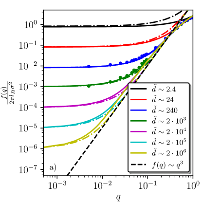
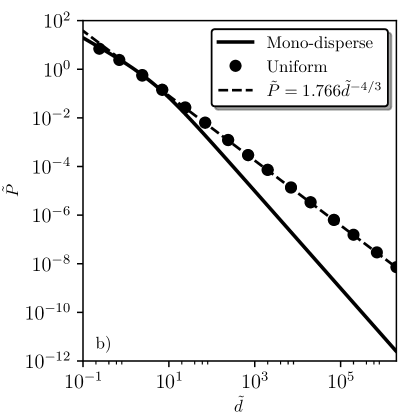
Figure 3: Flat polydispersity situation ($\gamma=0$, $\alpha=3$), meaning that $n(q)$ is uniform in the interval $[0,1]$, for the two-plates situation. a) Plot of the normalisation function $f(q)$, at different inter-plate distances. The circles are the estimates of $f(q)$ from the MC simulations. The solid lines show numerical results from the poly-disperse PB treatment and finally, the dot-dashed lines are for the analytic results using Eq. (82). This is complemented by the dashed black line indicating the analytic asymptotic Eq. (84). b) Equation of state. The black solid line is for the mono-disperse PB, black circles show the numerical results for the poly-disperse PB and the black dashed line is for the analytic prediction Eq. (90).

IV Discussion

In the present section, we first summarise our main findings and present a more heuristic derivation. This allows to generalise some of the two-plates results, that will then be tested against both Poisson-Boltzmann numerical solutions, and Monte Carlo simulations. We will also extend the analysis to a broader class of polydisperse distributions. Finally, we address a central question, establishing the connection between our continuous mixture results, and the properties that characterise discrete mixtures. Indeed, in any physically relevant system, $n(q)$ is discrete, with the result that the minimum charge cannot vanish. Yet, physics is governed, at large distances, by the small-$q$ features of $n(q)$, and more precisely, the new power-law regimes reported in previous sections are ruled by the vicinity of $q=0$. This raises a legitimate concern, and we explain in which sense the continuous limit is relevant to the discrete case.

IV.1 One-plate : summary of continuous distribution phenomenology

Our treatment elaborates on the one-plate situation, screened by counterions only. Some emphasis was put on the long-range behaviour, that is governed, expectedly, by the population of counterions having the smallest valence ($q_{\text{m}in}$). When $q_{\text{m}in}>0$, the system ultimately behaves like a monodisperse one, having counterions of valence $q_{\text{m}in}$. The one-plate density thus behaves at large distances $x$ like $x^{-2}$ and likewise, the two-plate pressure scales with distance $d$ like $d^{-2}$. Both function are furthermore independent of the plate’s bare charge $\sigma e$.

The situation changes when polydispersity is considered. We have introduced an important characteristics of polydispersity, through the exponent $\gamma$ specifying the low-$q$ behaviour of the valence distribution $n(q)$: $n(q)\propto\sigma q^{\gamma}$ for small $q$, where the surface charge density $\sigma$ is kept for dimensional reasons. We have $\gamma>-1$ to ensure normalisability. Decreasing $\gamma$ leads to an increase in the population of small $q$ counterions. These are less sensitive to the electric field of the plate, that they consequently screen less. Thus, the resulting one-plate electrostatic potential $\phi$ becomes longer range than in the monodisperse case, and behaves (in absolute value) like $x^{1/(\gamma+3)}$. Formally, the monodisperse case is recovered for $\gamma\to\infty$ (where the small $q$ regime is completely depleted), for which our formula yields $\phi\propto x^{0}$, hinting at a logarithmic dependence. For a given choice of index $\gamma$, we have shown that the counterionic number density $n(x)$ behaves (again at large $x$) like $x^{-2(\gamma+2)/(\gamma+3)}$, while the charge density displays a different scaling: $\rho(x)\propto x^{-(2\gamma+5)/(\gamma+3)}$. Again, when $\gamma\to\infty$, monodisperse phenomenology is recovered, with common asymptotic dependences for $n$ and $\rho$ in $x^{-2}$. The fact that the power-law exponent is $\gamma$ dependent immediately implies that the saturation feature discussed in section II is lost: when increasing $\sigma$, both $n(x)$ and $|\rho(x)|$ increase without bound: $n(x)\propto\sigma^{2/(\gamma+3)}$ and $|\rho(x)|\propto\sigma^{1/(\gamma+3)}$.

IV.2 Heuristic derivation of two plates scaling laws, and comparison to numerical results

The above one-plate considerations allow to recover some of our two-plates results, and to generalise them beyond the case $\gamma=0$ that was worked out in detail in section III. We again focus on the large-distance asymptotic, where in the vicinity of a given plate, the electrostatic potential is to a good approximation provided by its one-plate limit and thus behaves like $x^{1/(\gamma+3)}$. For finite $\gamma$, the key to the large-$d$ physics is that there is always a population of counterions that is too weakly charged to “feel” the electric potential. They have valence $q$ smaller than some $d$-dependent threshold $q^{*}$, that we can simply estimate by the following argument: $q^{*}\Delta\phi=1$, where $\Delta\phi$ is the potential difference between the plate-contact, and the mid-plate point. Thus, we get the crossover valence $q^{*}\propto d^{-1/(\gamma+3)}$. A relevant quantity is the total density of the corresponding essentially “free” counterions, $n_{f}$ given by $\int_{0}^{q^{*}}n(q)dq\propto(q^{*})^{1+\gamma}\propto d^{-(\gamma+1)/(\gamma+3)}$. These ions are the main contributors to the force/pressure between the two plates; having a surface density $n_{f}$ and a flat ($x$-independent) profile, their volume density is simply given by $n_{f}/d$, a quantity that gives the inter-plate pressure. We get here

$$P\,\propto\,\frac{n_{f}}{d}\,\propto\,d^{-2(\gamma+2)/(\gamma+3)}.$$ (91)

In the flat polydisperse $\gamma=0$ case, we recover the prediction $P\propto d^{-4/3}$ derived in section III, and confirmed by PB and MC simulations. Interestingly, we also retrieve the same functional dependence for the inter-plate pressure as the one-wall number density [same exponent $2(\gamma+2)/(\gamma+3)$, see Eq. (29)]. As a consequence, we can, along the same lines as in the monodisperse case, define a non-linear dimensionless ratio $\cal R_{\gamma}$, by comparing the true PB pressure at large $d$ to the superposition of the two one-plate densities at $d/2$. We have shown above that ${\cal R}_{\infty}=\pi^{2}/8$ (monodisperse situation). Computing $\cal R_{\gamma}$ requires the knowledge of all prefactors, which the present scaling analysis does not provide. Yet, the explicit results of section III for $\gamma=0$ yield ${\cal R}_{0}\simeq(3/2)^{2/3}\,1.766/2\simeq 1.157$, slightly smaller than ${\cal R}_{\infty}$, but again larger than unity. Assuming that ${\cal R}_{\gamma}$ remains close to 1 for other values, this would mean that the error incurred by computing the two-plate pressure at large $d$ from the superposition of the one-plate densities, results in an underestimation, but not larger than 25%.

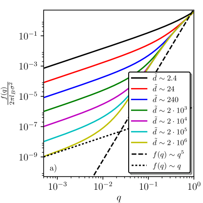
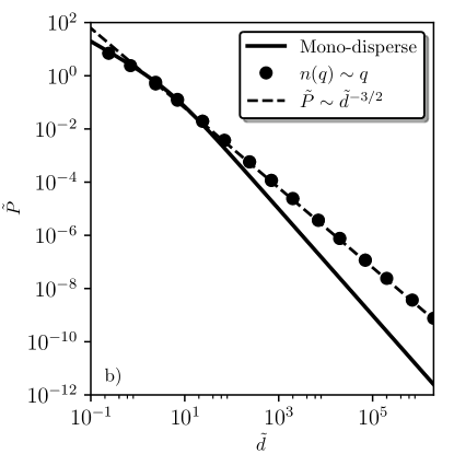
Figure 4: Skew distribution of counterions with $\gamma=1$, meaning that small $q$ ions are less numerous than ions with a larger $q$ (small$-q$ depleted distribution.) a) Plot of the normalisation function $f(q)$, at different distances. It can be seen that increasing $d$, $f$ adopts its one-plate shape in $q^{2\gamma+3}=q^{5}$ (see black dashed line), except below the threshold $q^{*}$ where it shows the same behaviour as the parent $n(q)$ (here linear in $q$) (see black dotted line). (Colored lines) as Fig. 3. b) Equation of state, which clearly shows a long-range $\tilde{d}^{-3/2}$-dependence, as predicted by Eq. (91). The symbols and curves have the same meaning as in Fig. 3.

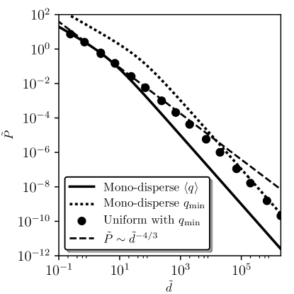
Figure 5: Poisson-Boltzmann equation of state for a uniform $n(q)$ with $q$ in the range $[0.05,1]$. Black circles show the numerical results for the poly-disperse PB. The two continuous curves show the PB monodisperse predictions, with two distinct Gouy lengths: (black solid line) for $\mu^{-1}=2\pi\ell_{\rm B}\sigma\langle q\rangle$, which is relevant at small distances, and (black dotted line) for $\mu^{-1}=2\pi\ell_{\rm B}\sigma q_{\text{m}in}$. These two curves have an asymptotic $1/d^{2}$ decay. An intermediate asymptotic with exponent $4/3$ sets in (dashed line).

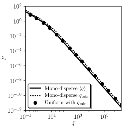
Figure 6: Same as Fig. 5, for a uniform $n(q)$ with $q$ in the range $[0.5,1]$

In Fig. 4, we show numerical PB results for $\gamma=1$, with thus less small $q$ counterions than the $\gamma=0$ distribution discussed earlier. As a consequence, the pressure exhibits a faster decay with $d$, predicted to be $d^{-3/2}$, see Eq. (91). This is fully confirmed in Fig. 4. In addition, we have tested a number of expectations, shaped on our previous analysis. First of all, all distribution $n(q)$ having non-vanishing $n(0)$ should display the same large-distance pressure, that of the $\gamma=0$ class. This was checked for the choice $n(q)\propto(q_{\rm max}-q)$ (results not shown). Second, all distributions depleted near the origin ($n(q)=0$ for some range $q<q_{\text{m}in}$) should asymptotically behave like a monodisperse system, with counterion valence $q_{\text{m}in}$. Yet, if $q_{\text{m}in}$ is not too large, the system should require large distances $d$ before “realising” that $q_{\text{m}in}$ is actually non vanishing. We should thus expect a cross-over between the finite $\gamma$ behaviour in some intermediate $d$-range, and the $\gamma=\infty$ ultimate decay. This is what Fig. 5 clearly illustrates. On the other hand, if $q_{\text{m}in}$ and the maximum valence $q_{\text{m}ax}$ are not separated enough, the behaviour is of course close to its monodisperse counterpart. Fig. 6 shows that it is already the case when $q_{\text{m}ax}/q_{\text{m}in}=2$. Finally, we show in Fig. 7 that for quite a large class of polydispersities, although the large-$d$ asymptotic may be $n(q)$-dependent, the behaviour of pressure at smaller distances is made rather universal, using properly scaled quantities TrST16 . The data collapse reported is quite striking at short distances. For large $d$, the collapse is necessarily broken, since the different distributions studied correspond to distinct types, with various $\gamma$ exponents. The corresponding decays range from $d^{-4/3}$ to $d^{-2}$, including $d^{-3/2}$. It is at this point relevant to stress that this collapse holds beyond the mean-field regime which has been under scrutiny here, as revealed in Fig. 8 by Monte Carlo simulations for two strong coupling cases at various counterion mixtures. The negative pressures seen at these high coupling parameters are a consequence of the now well-known ion-ion correlations, which is omitted in our mean-field treatment. Surprisingly, these correlations do not break the collapse. These ion-ion correlations, that increase with the coupling parameter, can turn repulsive electrostatic interactions between two equally charged surfaces into attractive ones. Even though the chosen coupling parameters are above realistic values for an aqueous electrolyte system (to be sure that the system is indeed dominated by ion-ion correlation effects), we emphasize that the same data-collapse holds for more experimentally relevant coupling parameters TrST16 . In addition, we address the possibility of a broader universality, including the tail of the equation of state, in the following subsection.

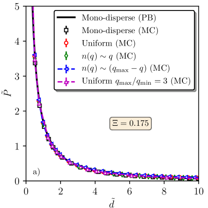
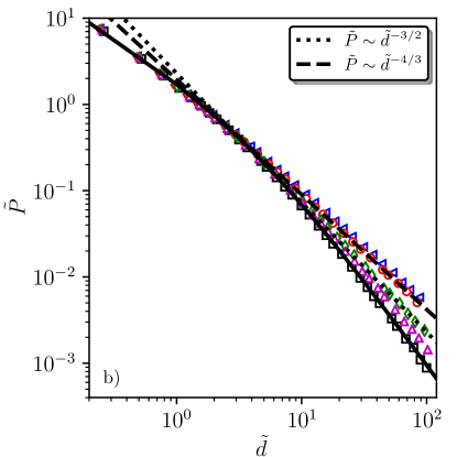
Figure 7: Equation of state versus distance (where $\widetilde{d}$ is defined as $2\pi\ell_{\rm B}\sigma\langle q\rangle\,d$)), for various valence distributions: mono-disperse, uniform, skewed $n(q)\sim q$ (up to an upper cutoff), skewed $n(q)\sim(q_{\rm max}-q)$ (up to an upper cutoff), and uniform in $[q_{\rm min},q_{\rm max}]$ with $q_{\rm min}\neq 0$. The MC simulations are run at a coupling constant $\Xi=0.175$.

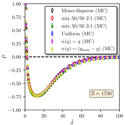
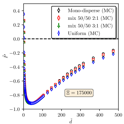
Figure 8: Monte Carlo reduced pressure versus normalized separation, for strongly coupled systems ($\Xi=1750$ and $175000$) for which the Poisson-Boltzmann theory analysed in this paper would completely fail. Significantly different distributions $n(q)$ are considered : monodisperse, bidisperse with $q_{\text{m}in}/q_{\text{m}ax}=1/2$, $q_{\text{m}in}/q_{\text{m}ax}=1/3$, continuous ($q_{\text{m}in}$=0, $\gamma=0$), and skewed (as in Fig. 7).

IV.3 From continuous to discrete distribution of charges

So far, we only considered continuous distributions of charges $n(q)$, and we established the connection between the behaviour of $n(q)$ for $q\to 0$, and the long-range pressure or ionic profiles. This may seem rather academic since any real physical system will exhibit some discreteness in $n(q)$. Our treatment thus raises a two-pronged question: first, how “close to continuous” should a discrete $n(q)$ be to exhibit the predicted behaviour? Second, since the tail of the density profile (one-plate case), or the long-distance equation of state (two plates) is necessarily ruled by the smallest charges in the system, how can the continuous power-laws derived for $q_{\text{m}in}=0$ be observed in a discrete system having necessarily $q_{\text{m}in}>0$? We note here that if a species with a strictly vanishing charge is present in the mixture, it is simply discarded by the analytical treatment worked out here.

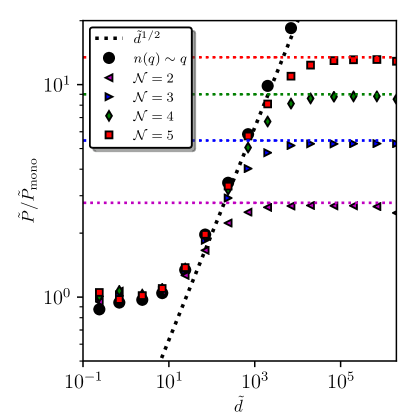
Figure 9: Normalized pressure $\tilde{P}/\tilde{P}_{\text{m}ono}$ as obtained from the poly-disperse Poisson-Boltzmann, where $\tilde{P}_{\text{m}ono}$ is associated to a monodisperse system, with thus long-distance decay in $\tilde{d}^{-2}$. Five discrete $n(q)$ are considered with different number of species $\cal N$. The 1-2 system has charges 1/2 and 1 (${\cal N}=2$, $q_{\text{m}in}=1/2$), the 1-3 system features charges 1/3, 2/3 and 1 (${\cal N}=3$, $q_{\text{m}in}=1/3$) etc, and the 1-5 system is with charges 1/5, 2/5,… 1. In all cases, the distribution is skewed, so that $n(q)\propto q$. As more and more species are added in the mixture, a transient asymptotic sets in (dotted line), which exactly matches the continuous limiting distribution (obtained for ${\cal N}\to\infty$, see the bullets). The value of the horizontal plateaus is given in the text.

Fig. 9 shows a rather striking result, establishing the proximity between the discrete and continuous cases. The pressure arising in the Poisson-Boltzmann framework is computed for a number of mixtures, having $\cal N$ different species, with equispaced charges (like with a mixture of ions having integer charge values), and such that the number density of a constituent scales like $q$ itself (skewed distribution). This means that the index $\gamma$ introduced above is unity, and we expect a large distance pressure in $d^{-3/2}$ for the continuous mixture with $q_{\text{m}in}=0$ (see Eq. (91)). Since we show $P$ normalised by the monodisperse reference case, the continuous power-law for $P/P_{\text{m}ono}$ should be in $d^{1/2}$ (dotted line), in good agreement with the disc symbols on the figure. On the other hand, all discrete mixtures should asymptotically behave, scaling-wise, like their monodisperse counterpart, at distances when only $q_{\text{m}in}$ does remain in the solution. This means that $P/P_{\text{m}ono}$ in Fig. 9 is expected to flatten at large $d$, and converge towards a simple value: from our choice of units, $\langle q\rangle^{2}/q_{\text{m}in}^{2}$ (e.g., $9/4$ for ${\cal N}=2)$, in perfect agreement with the numerical data. Yet, the most interesting feature is that for ${\cal N}=5$ already, the “continuous” power-law is clearly visible, not asymptotically of course, but transiently (and for about a decade in distance). Fig. 9 thereby shows how the continuous limit results are recovered upon increasing ${\cal N}$, and that an arguably small value of ${\cal N}$ is sufficient to exhibit some of the hallmarks of continuous systems.

Fig. 10 illustrates a similar effect, with the distinction that all distributions shown share the same value of $q_{\text{m}in}$, even the continuous case. Here, we chose a “flat” situation where $n(q)$ is the same for all $q$ values. The first message conveyed is that all curves are reasonably close (and all the closer as we are displaying data on a log scale), so that discreteness effects are not paramount. While the ${\cal N}=20$ charges case is arguably close to the continuous limit, considering ${\cal N}=2-3$ peaks is already sufficient to observe the main trend. The second message pertains to the transient asymptotic. In Fig. 10, the dashed line with slope $-4/3$ is the prediction derived in this work (corresponding to $\gamma=0$ and $q_{\text{m}in}=0$). While all distributions yield a large $d$ tail in $d^{-2}$ since $q_{\text{m}in}\neq 0$, the “continuous/$q_{\text{m}in}=0$” power-law in $d^{-4/3}$ does hold approximately in a finite distance range, over 4 decades. The salient features of Fig. 9 and 10 explain why the analytical derivations proposed here have relevance for discrete systems as well.

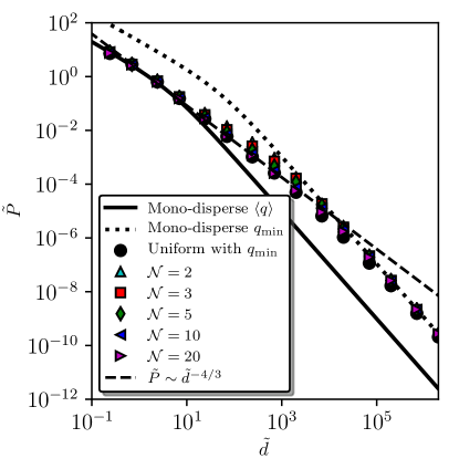
Figure 10: Illustration of quasi-universality for different distributions exhibiting the same value of $q_{min}$. Five discrete distributions are considered, with equidistributed charges starting at $q_{\text{m}in}=0.05$ and such that $\langle q\rangle=1/2$, and ${\cal N}=2$, 3, 5, 10 and 20 charges. The pressure is compared to those of the corresponding continuous model ${\cal N}\to\infty$, and of the two limiting monodisperse regimes: one with $n(q)=\delta(q-1/2)$ (lower bound shown by the continuous line), and the other for $n(q)=\delta(q-0.05)$ (upper bound, dotted line).

Appendix A One-plate geometry : long-range features

In this appendix, we establish the connection between the small $q$-behaviour of function $f(q)$ as encoded in Eq. (26), with the long-distance regime of densities (charge, and number densities, that do differ in general). Injecting (26) into (24), we get

$$\left[\phi^{\prime}(\widetilde{x})\right]^{2}=\frac{4}{\langle q\rangle^{2}}a\Gamma(\alpha+1)\frac{1}{[-\phi(\widetilde{x})]^{\alpha+1}},\qquad\widetilde{x}\to\infty,$$ (92)

where $\Gamma$ denotes the Gamma function. The solution of this asymptotic equation is searched in the form

$$\phi(\widetilde{x})\mathop{\sim}_{\widetilde{x}\to\infty}-b\left(\frac{\widetilde{x}}{\langle q\rangle}\right)^{\beta}.$$ (93)

Inserting this ansatz into Eq. (92), the exponent $\beta$ and the prefactor $b$ are determined self-consistently as

$$\beta=\frac{2}{\alpha+3},\qquad b^{\alpha+3}=a\Gamma(\alpha+1)(\alpha+3)^{2}.$$ (94)

The large-distance behaviour of the electric potential reads

$$\phi(\widetilde{x})\mathop{\sim}_{\tilde{x}\to\infty}-\left[a\Gamma(\alpha+1)(\alpha+3)^{2}\right]^{\frac{1}{\alpha+3}}(\widetilde{x}/\langle q\rangle)^{\frac{2}{\alpha+3}}.$$ (95)

The logarithmic dependence found in the monodisperse case for $\phi$ changes to an asymptotic power-law behaviour with non-universal index and prefactor, depending on the model’s parameters $a$ and $\alpha$. This is the consequence of a less efficient screening with counterions having a small $q$. As we shall see below, large-$\beta$ values correspond to systems with enhanced population with $q$ near 0, with resulting impeded screening. The asymptotic number density profile of particles reads as

$$n(\widetilde{x}) = \int_{0}^{1}{\rm d}q\,f(q){\rm e}^{q\phi(\tilde{x})}\mathop{\sim}_{\tilde{x}\to\infty}2\pi\ell_{\rm B}\sigma^{2}a\frac{\Gamma(\alpha+1)}{[-\phi(\widetilde{x})]^{\alpha+1}}$$ (96)

$$= 2\pi\ell_{\rm B}\sigma^{2}\frac{[a\Gamma(\alpha+1)]^{\frac{2}{\alpha+3}}}{(\alpha+3)^{2\left(\frac{\alpha+1}{\alpha+3}\right)}}\frac{1}{(\widetilde{x}/\langle q\rangle)^{2\left(\frac{\alpha+1}{\alpha+3}\right)}}.$$

Similarly, the asymptotic charge density profile reads as

$$\frac{\rho(\widetilde{x})}{(-e)} = \int_{0}^{1}{\rm d}q\,qf(q){\rm e}^{q\phi(\tilde{x})}\mathop{\sim}_{\widetilde{x}\to\infty}2\pi\ell_{\rm B}\sigma^{2}a\frac{\Gamma(\alpha+2)}{[-\phi(\widetilde{x})]^{\alpha+2}}$$ (97)

$$= 2\pi\ell_{\rm B}\sigma^{2}\frac{[a\Gamma(\alpha+1)]^{\frac{1}{\alpha+3}}(\alpha+1)}{(\alpha+3)^{2\left(\frac{\alpha+2}{\alpha+3}\right)}}\frac{1}{(\widetilde{x}/\langle q\rangle)^{2\left(\frac{\alpha+2}{\alpha+3}\right)}}.$$

It is easy to check that these asymptotic behaviours fulfil the exact relation $\rho(\widetilde{x})/(-e)=n^{\prime}(\widetilde{x})/\phi^{\prime}(\widetilde{x})$, see Eq. (17). We conclude that the non-universal large-$x$ behaviour of the reduced potential, the number and charge density profiles are determined by the small-$q$ behaviour of the normalisation function $f(q)$. This was expected, since those counterions with the smallest $q$ are the least sensitive to the created electric field, and thus the most delocalised.

Let us rewrite the $n-f$ relation (18) in terms of the dimensionless $\widetilde{x}$,

$$\frac{n(q)}{\sigma}=\frac{f(q)}{2\pi\ell_{\rm B}\sigma^{2}}\int_{0}^{\infty}\frac{{\rm d}\widetilde{x}}{\langle q\rangle}\,{\rm e}^{q\phi(\tilde{x})}.$$ (98)

In the limit $q\to 0$, we can use the small-$q$ asymptotic (26) in Eq. (98) to write down

$$\frac{n(q)}{\sigma}\mathop{\sim}_{q\to 0}aq^{\alpha}\int_{0}^{\infty}\frac{{\rm d}\widetilde{x}}{\langle q\rangle}\,{\rm e}^{q\phi(\tilde{x})}.$$ (99)

The integral on the rhs of this equation diverges as $q\to 0$ due to the integration of unity over an infinite support. We do not know the functional form of the reduced potential $\phi$ at small $\widetilde{x}$, but we do know its asymptotic form (95) at large $\widetilde{x}$. Since the integral diverges, any integration on a finite interval does not affect the leading divergent term. Based on this fact we make an assumption which will be later verified numerically on a specific model: to study the small-$q$ divergence of the integral in (99) it is sufficient to insert there the asymptotic large-$\widetilde{x}$ formula for the potential (95). If this assumption is correct, we obtain

$$\int_{0}^{\infty}\frac{{\rm d}\widetilde{x}}{\langle q\rangle}\,{\rm e}^{q\phi(\tilde{x})}\mathop{\sim}_{q\to 0}\frac{1}{2}\frac{1}{\sqrt{a\Gamma(\alpha+1)}}\Gamma\left(\frac{\alpha+3}{2}\right)q^{-\frac{\alpha+3}{2}}.$$ (100)

Consequently,

$$\frac{n(q)}{\sigma}\mathop{\sim}_{q\to 0}\frac{1}{2}\sqrt{\frac{a}{\Gamma(\alpha+1)}}\Gamma\left(\frac{\alpha+3}{2}\right)q^{\frac{\alpha-3}{2}}.$$ (101)

We see that in the $q\to 0$ limit, the density distribution goes to a nonzero constant when $\alpha=3$, it vanishes when $\alpha>3$ and diverges for $\alpha<3$. Since the surface density of particles must be finite, the density distribution should be integrable for small $q$ and we have the restriction $\alpha>1$.

The crucial relation (101) relates the small-$q$ behaviour of the density function of particles $n(q)$, which is given from the outset in the direct formulation of the problem, to the small-$q$ behaviour of the normalisation function $f(q)$ (26). It turns convenient to introduce a parameter $\gamma$ through

$$\alpha=2\gamma+3,\qquad a=c^{2}\frac{2^{2\gamma+5}}{\sqrt{\pi}}\frac{\Gamma\left(\gamma+\frac{5}{2}\right)}{(\gamma+2)\Gamma(\gamma+3)}.$$ (102)

Indeed, $\gamma$ characterises the behaviour of $n(q)$ at small $q$, which is physically more relevant that the behaviour of $f(q)$, see the main text.

Appendix B Computational aspects

B.1 Poisson-Boltzmann resolution

The polydisperse Poisson-Boltzmann equation, Eq. (43), was solved numerically through a real-valued variable-coefficient ordinary differential equation (ODE) solver with an initial guess of $f_{g}(q)$-distribution aimed to target a particular $n_{t}(q)$-distribution. For each such $f_{g}(q)$ guess, a new corresponding $n_{g}(q)$-distribution is found through Eq. (63). A new guess for the correct $f_{t}(q)$-distribution is then generated by a mixing of the new distribution $f_{g,{\rm new}}(q)$ with the old one, $f_{g,{\rm old}}(q)$. The new $f_{g,{\rm new}}(q)$-distribution is found from a re-distribution of the old $f_{g,{\rm old}}(q)$ through

$$f_{g,{\rm new}}(q)=f_{g,{\rm old}}(q)\frac{n_{t}(q)}{n_{g}(q)}.$$ (103)

Mixing of $f_{g,{\rm old}}(q)$ and $f_{g,{\rm new}}(q)$ is then done with a small fraction of the new guess compared to the old. However, such a mixing of $f(q)$ runs into the risk of creating unrealistic negative values of pressures and imaginary electrostatic potentials (see e.g. Eq. (44)). To avoid such negative pressures a renormalisation of the total distribution $f(q)$ is performed using Eq. (44) such that the pressure at contact matches the pressure calculated from the mid-plane. Such a scheme usually reaches a convergence just after a few iterations. Consistency was then checked by calculating the pressure through the two pressure routes, at contact and across the mid-plane according to Eq. (44).

Alternatively one can solve the second order ODE, instead of the redefined first order ODE, for the poly-disperse case according to Eq. (20), but at the expense of time to convergence. Both routes yield however the same results. A typical calculation was based on a discretisation of $q$, $n(q)$, and $f(q)$ into 1000 bins as well as discretisation of the $x$ axis (usually by some fractions of $\ell_{\rm B}$). We verified that our solutions did not depend on these discretizations/binnings by increasing or decreasing the number of bins/steps.

B.2 Monte Carlo simulations

We have performed Monte-Carlo simulations in a quasi-2D geometry. Long-ranged electrostatic interactions are handled with Ewald summation techniques corrected for quasi-2D-dimensionality by introducing a vacuum slab in the $z$-direction perpendicular to the surfaces Berkowitz ; Mazars . We verified that our vacuum slab is sufficiently wide, so as not to influence the results. All simulations consisted of 512 point charges while the surfaces are modelled as structureless infinite plates with uniform surface charge densities equal to $\sigma e$. Simulations were performed both for discrete mixtures of charges as well as for quasi-continuous distributions of charges, $q\in[q_{\rm min},q_{\rm max}]$. Standard displacement trials were performed with an acceptance ratio of around 30%. Pressures were estimated using the contact densities and the contact theorem as well as across the mid-plane, and were collected over $10^{5}$ Monte Carlo cycles. These two approaches yielded the same pressures within statistical noise/errors. Estimates of $f(q)$ for each mixture was done by measuring the contact values at the wall for each $q$-values (via a discretisation). To be able to compare with our Poisson-Boltzmann calculations, we have performed the simulations at sufficiently low coupling parameter ($\Xi=0.175$). To show quasi-universality also beyond mean-field we have performed simulations at higher coupling parameters ($\Xi=1750$ and $\Xi=175000$).

References

- (1)
- (2) Ivlev A., Löwen H., Morfill G. and Royall C. P., Complex Plasmas and Colloidal Dispersions: Particle-resolved studies of Classical Liquids and Solids (World Scientific, Singapore, 2012).
- (3) Tata B R V and Arora A K, 1995 J. Phys.: Cond. Matter 20 3817
- (4) van der Linden M. N., van Blaaderen A., and Dijkstra M., 2013 J. Chem. Phys. 138 114903
- (5) Auer S. and Frenkel D., 2001 Nature 413 711
- (6) Berthier L., Chaudhuri C., Coulais C., Dauchot O., and Sollich P.. 2011 Phys. Rev. Lett. 106 120601
- (7) Bartlett P., 2000 J. Phys.: Condens. Matter 12 A275
- (8) Sollich P., and Wilding N. B., 2011 Soft Matter 7, 4472
- (9) Eldridge M. D., Madden P. A. and Frenkel D., 1993 Nature 365 35
- (10) Botet R., Cabane B., Goehring L., Li J. and Artzner F., 2016 Faraday Discuss. 186, 229
- (11) Zhang J., Blaak R., Trizac E., Cuesta J. A. and Frenkel D., 1999 J. Chem. Phys. 110 5318
- (12) Blaak R. and Cuesta J. A., 2001 J. Chem. Phys. 115 964
- (13) Anderson C. F. and Record Jr M. T., 1980, Biophys. Chem. 11 353
- (14) Durand-Vidal S., Turq P., Marang L,, Pagnoux C. and Rosenholm J. B., 2005 Coll. Surfaces A: Physicochem Eng. Aspects, 267 117
- (15) Ryzhkova A. V.,Skarabot M. and I. Musevic M., 2015 Phys. Rev. E 91, 042505
- (16) Levin Y., 2002 Rep. Prog. Phys. 65 1577
- (17) Ulander J., Greberg H., and Kjellander R., 2001 J. Chem. Phys. 115 7144
- (18) Téllez G., and Trizac E., 2004 Phys. Rev. E 70 011404
- (19) Téllez G., and Trizac E., 2006 Phys. Rev. Lett. 96, 038302
- (20) Gouy G L, 1910 J. Phys. 9 457
- (21) Tracy C. A. and Widom H., 1997 Physica A 244, 402
- (22) Palberg T., Medebach M., Garbow N., Evers M., Barreira Fontecha A., Reiber H. and Bartsch E., 2004 J. Phys.: Condens. Matt. 16, S4039
- (23) Andelman D, in Soft Condensed Matter Physics in Molecular and Cell Biology, Chapter 6, pp 98-122, edited by Poon W C K and Andelman D (Taylor & Francis, New York, 2006)
- (24) Chapman D L, 1913 Philos. Mag. 25 475
- (25) Naji A., Jungblut S., Moreira A. G., and Netz R. R., 2005 Physica A 352 131
- (26) Šamaj L. and Trizac E., 2011 Phys. Rev. Lett. 106, 078301
- (27) It should be kept in mind that the accuracy of PB theory deteriorates upon increasing the electrostatic coupling strength , and that increases with counterion valence.
- (28) Henderson D. and Blum L., 1978 J. Chem. Phys. 69 5441
- (29) Henderson D., Blum L. and Lebowitz J. L, 1979 J. Electroanal. Chem. 102 315
- (30) Choquard P., Favre P. and Gruber C., 1980 J. Stat. Phys. 23 405
- (31) Carnie S. L. and Chan D. Y. C., 1981 J. Chem. Phys. 74 1293
- (32) Totsuji H., 1981 J. Chem. Phys. 75 871
- (33) Wennerström H., Jönsson B. and Linse P., 1982 J. Chem. Phys. 76 4665
- (34) Mallarino J.-P., Téllez G. and Trizac E., 2015 Mol. Phys. 113 2409
- (35) Bocquet L., Trizac E. and Aubouy M., 2002 J. Chem. Phys. 117 8138
- (36) Téllez G. and Trizac E., 2003 Phys. Rev. E 68, 061401
- (37) Trizac E. and Šamaj L., Lecture notes for the International School on Physics Enrico Fermi, Physics of Complex Colloids, Varenna 2012, organized by C. Bechinger, F. Sciortino, and Primoz Ziherl; Proceedings of Course CLXXXIV; arXiv:1210.5843
- (38) Trulsson M., Šamaj L. and Trizac E., 2017 Europhys. Lett. 118 16001
- (39) Yeh I.-C. and Berkowitz M. L., 1999 J. Chem. Phys. 111, 3155
- (40) Mazars M., Caillol J.-M., Weis J.-J., and Levesque D., 2001 Condens. Matter Phys. 4, 697