Floquet Weyl semimetals in light-irradiated type-II and hybrid line-node semimetals

Abstract

Type-II Weyl semimetals have recently attracted intensive research interest because they host Lorentz-violating Weyl fermions as quasiparticles. The discovery of type-II Weyl semimetals evokes the study of type-II line-node semimetals (LNSMs) whose linear dispersion is strongly tilted near the nodal ring. We present here a study on the circularly polarized light-induced Floquet states in type-II LNSMs, as well as those in hybrid LNSMs that have a partially overtilted linear dispersion in the vicinity of the nodal ring. We illustrate that two distinct types of Floquet Weyl semimetal (WSM) states can be induced in periodically driven type-II and hybrid LNSMs, and the type of Floquet WSMs can be tuned by the direction and intensity of the incident light. We construct phase diagrams of light-irradiated type-II and hybrid LNSMs which are quite distinct from those of light-irradiated type-I LNSMs. Moreover, we show that photoinduced Floquet type-I and type-II WSMs can be characterized by the emergence of different anomalous Hall conductivities.

I Introduction

Topological semimetals represent a new class of topological matter, which is characterized by a gapless bulk with a nontrivial band topology. A Weyl semimetal (WSM) is a kind of topological semimetal that supports Weyl fermions as low-energy excitations. According to the electronic band structures, WSMs can be divided into three distinct types: a type-I WSM that has a pointlike Fermi surface WanX11PRB ; YangKY11PRB ; Huang15NatCommun ; Weng15PRX , a type-II WSM whose Fermi surface consists of an electron pocket and a hole pocket touching at the Weyl nodes SoluyanovAA15Nature ; XuY15PRL , and a hybrid WSM in which one Weyl node belongs to type I whereas its chiral partner belongs to type II LiFY16PRB . Earlier research interests were mainly concentrated on type-I WSMs since real type-I WSM materials had been theoretically proposed Huang15NatCommun ; Weng15PRX and experimentally confirmed in inversion-symmetry-breaking TaAs-class crystalsXuSY15Science ; LvBQ15PRX ; XuSY15NatPhys ; Yang15NatPhys . When Lorentz invariance is broken, Weyl cones may be tipped over and transformed into type II. Recently, promising materials such as MoTe₂ and WTe₂ have been proposed to be type-II WSMsSoluyanovAA15Nature ; WangC16PRB ; BrunoFY16PRB ; WuY16PRB ; FengB16PRB ; SunY15PRB ; WangZ16PRL , and experimental confirmations of MoTe₂ have been reportedDengK16NatPhys ; Huang16NatMaterials . Additionally, it was reported that we can convert TaAs and WTe₂ into hybrid WSMs by doping with magnetic ions and creating magnetic orders in them LiFY16PRB .

Another kind of topological semimetal is the so-called line-node semimetal (LNSM). Unlike WSMs in which the conduction band touches the valence band at discrete points in momentum space, in LNSMs the conduction band and the valence band touch along lines. In analogy to WSMs, according to the tilting degree of the band spectra around the nodal rings, LNSMs can also be classified into type-I, type-II, and hybrid categories. To date, type-I LNSMs have been intensively studied both theoretically Heikkila11JETP ; Burkov11PRB ; Chiu11PRB ; ChanYH16PRB ; Chiu15PRB ; Fang15PRB ; Ali14PRB ; Xie15APL ; Kim15PRL ; Yu15PRL ; Bian16PRB ; Weng16JPCM ; Huang16PRB ; Mullen15PRL ; Bian16NatComm ; Schoop16NatCommun and experimentally Xie15APL ; Bian16NatComm ; Schoop16NatCommun ; Neupane16PRB ; Wu16NatPhys ; Hu16PRL ; Takane16PRB , however, research on type-II LNSMs is just beginning Hyart16PRB ; Volovik17JLTP ; LiS17PRB ; ZhangX17JPCL ; HeJ17Arxiv ; GaoY17Arxiv . The very recent angle-resolved photoemission spectroscopy measurements on Mg₃Bi₂ suggest it to be a promising candidate material for a type-II LNSM Chang17Arxiv . As far as we know, the hybrid LNSM, characterized by a partially overtilted linear dispersion in the vicinity of the nodal ring, has yet to be proposed and studies are lacking. Type-I LNSMs exhibit intriguing physical phenomena such as a three-dimensional (3D) quantum Hall effect Mullen15PRL , 3D flat Landau levels Rhim15PRB , $n^{1/4}$ dependence of the plasmon frequency on the charge concentration in the long-wavelength limit Rhim16NJP ; Yan16PRB , and a quasitopological electromagnetic response Ramamurthy17PRB . Owing to peculiar band spectra, type-II and hybrid LNSMs are expected to display more intriguing phenomena.

Application of light offers a powerful method to manipulate electronic states, and even change the band topology in solids WangY13Science ; Mahmood16NatPhys ; SieEJ15NatureMater ; KimJ14Science . A typical example is the Floquet topological insulator Lindner11NatPhys ; Titum17PRB ; Titum15PRL , which is a direct consequence of changing the band topology by means of light. Moreover, photoinduced topological states in other two-dimensional systems, such as graphene Oka09PRB ; KitagawaT11PRB ; GuZ11PRL ; Piskunow14PRB and siliceneEzawa13PRL , have been studied. Recently, light-driven semimetals have attracted much attentionWangR14EPL ; Chan16PRL ; Ebihara16PRB ; Chan16PRB ; YanZ16PRL ; Narayan16PRB ; Taguchi16PRB1 ; Ezawa17PRB ; YanZ17PRB1 ; YaoS17PRB ; YanZ17PRB2 ; Klinovaja17PRL ; Bomantara16PRBE ; Chan17PRB . It was found that a Floquet WSM phase can be generated from a light-driven Dirac semimetal due to time-reversal symmetry breaking WangR14EPL ; Chan16PRL ; Ebihara16PRB ; Chan16PRB . Later, it was shown that circularly polarized light can drive a type-I LNSM into a WSM, accompanied by photovoltaic anomalous Hall conductivity Chan16PRB ; YanZ16PRL ; Narayan16PRB ; Taguchi16PRB1 ; Ezawa17PRB . A Floquet WSM phase with multi-Weyl points was also proposed in crossing LNSMsYanZ17PRB1 ; YaoS17PRB ; YanZ17PRB2 .

In this paper, we present a systematic study on Floquet states in periodically driven type-II [Fig. 1(a₃)] and hybrid [Fig. 1(a₂)] LNSMs by means of light. We show that Floquet WSMs can be created by applying circularly polarized light. When the incident light propagates along the $x$ axis or along the $z$ axis, a type-II LNSM is converted into a type-II WSM [Figs. 1(b₃) and 1(d₃)], while for a driven hybrid LNSM, depending on the tilt direction, the photoinduced Floquet WSM could be of type I [Fig. 1(b₂)] or type II [Fig. 1(d₂)]. When the applied light propagates along the $y$ axis, only the positions of the nodal rings change [Figs. 1(c₂) and 1(c₃)]. Surprisingly, by rotating incident light on the $x$-$z$ plane, both type-I and type-II WSMs can be realized by tuning the driving angle and amplitude [Figs. 1(e₂) and 1(e₃)]. For the sake of comparison, we also give the Floquet states of driven type-I LNSMs by circularly polarized light [Figs. 1(a₁)-1(e₁)] which show different features from those of type-II and hybrid LNSMs. We summarize all the results in three distinct phase diagrams in ($A_{L}$, $\psi$) space, where $A_{L}$ and $\psi$ are the amplitude and the incident angle, respectively. Lastly, by use of the Kubo formula, the anomalous Hall effect of photoinduced Floquet WSMs is also investigated.

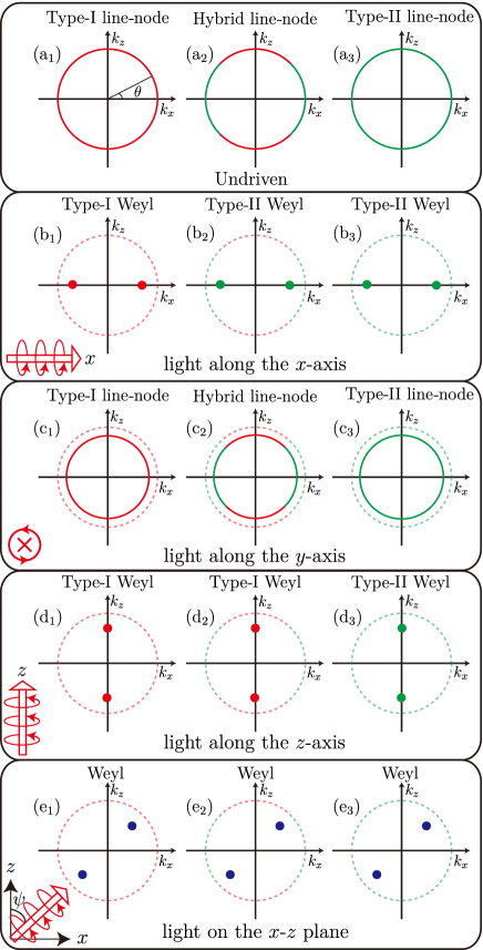
Figure 1: (Color online) Schematics of driven type-I, hybrid, and type-II LNSMs. (a) Nodal rings of undriven LNSMs. (b) and (d) correspond to the case where the incident light travels along the $x$ axis and $z$ axis, respectively. The dots colored with red (or green) denote type-I (or II) Weyl nodes. Nodal rings are gapped out and Weyl nodes are created along the propagation direction of light. (c) The incident light along the $y$ axis only shifts the nodal rings. (e) The light propagates on the $x$-$z$ plane, with $\psi$ defining the incident angle away from the $z$ axis. Nodal rings are gapped out and pairs of Weyl nodes appear along the propagation direction. We label the Weyl nodes with blue color as their type depends on the model parameters, the incident angle and the strength of light. The dashed lines in (b)-(e) correspond to nodal rings in the undriven cases.

II Model

To study periodically driven LNSMs, we start with a simple two band model of LNSMs with a single nodal ring. The model Hamiltonian of undriven LNSMs is written asKim15PRL ; Yu15PRL ; WengH15PRB ; Chan16PRB

$$H_{0}=c_{i}k_{i}^{2}\sigma_{0}+\left(m_{0}-m_{i}k_{i}^{2}\right)\sigma_{z}+v_{y}k_{y}\sigma_{y},$$ (1)

where $m_{0},m_{i}(i=x,y,z)$ and $c_{i}$ are model parameters, $v_{y}$ is the velocity along the $y$-axis, $k_{i}$ are the crystal momenta, $\sigma_{i}$ are Pauli matrices and $\sigma_{0}$ is the identity matrix. We use Einstein’s summation convention that repeated indices indicate the summation is implied. This model respects both the time-reversal and inversion symmetries, thus can be applied to spinless LNSM systemsKim15PRL ; WengH15PRB ; Yu15PRL . The eigenvalues are obtained by diagonalizing the Hamiltonian (1),

$$E_{\pm}^{0}\left(\mathbf{k}\right)=c_{i}k_{i}^{2}\pm\sqrt{\left(m_{0}-m_{i}k_{i}^{2}\right)^{2}+v_{y}^{2}k_{y}^{2}}.$$ (2)

Under the band inversion condition $m_{0,x,y,z}>0$, a nodal ring appears along an ellipse defined by $m_{x}k_{x}^{2}+m_{z}k_{z}^{2}=m_{0}$ at $k_{y}=0$. The nodal ring is located at $\mathbf{k}_{0}=\left(\sqrt{m_{0}/m_{x}}C_{\theta},0,\sqrt{m_{0}/m_{z}}S_{\theta}\right),$ where $C_{\theta}=\cos\theta$, $S_{\theta}=\sin\theta$, and $\theta$ is the polar angle shown in Fig. 1(a₁). Linearizing the eigenvalues around the nodal ring we get the energy dispersion

$$E_{\pm}^{0}\left(\mathbf{q}=\mathbf{k}-\mathbf{k}_{0}\right) =\bm{w}\cdot\mathbf{q}\pm\sqrt{\left(\xi_{x}q_{x}+\xi_{z}q_{z}\right)^{2}+\xi_{y}^{2}q_{y}^{2}}$$

$$=T\left(\mathbf{q}\right)\pm U\left(\mathbf{q}\right),$$ (3)

where $\xi_{x}^{2}=4m_{0}m_{x}C_{\theta}^{2}$, $\xi_{y}^{2}=v_{y}^{2}$, $\xi_{z}^{2}=4m_{0}m_{z}S_{\theta}^{2}$, and $\bm{w}=2\left(c_{x}C_{\theta}\sqrt{m_{0}/m_{x}},0,c_{z}S_{\theta}\sqrt{m_{0}/m_{z}}\right)$. The first $T$ term of Eq. (3) describes the tilt of the energy dispersion, and the second $U$ term of Eq. (3) denotes the splitting of the energy band. Around point $\mathbf{k}_{0}$ on the nodal ring, we obtain a two dimensional Dirac cone when the small vector $\mathbf{q}$ is confined on the transverse plane formed by the inplane normal line to the nodal ring and the line along the $k_{y}$ axis. From Eq. (3), we can see that the tilt is most effective when $\mathbf{q}$ is along the direction of normal vector $\mathbf{k}_{n}=(m_{x}k_{0x},m_{z}k_{0z})$, then the tilt radio can be defined by SoluyanovAA15Nature ; LiS17PRB

$$F_{\theta}=\left|\frac{T(\hat{\mathbf{k}}_{n})}{U(\hat{\mathbf{k}}_{n})}\right|=\left|\frac{c_{x}C_{\theta}^{2}+c_{z}S_{\theta}^{2}}{m_{x}C_{\theta}^{2}+m_{z}S_{\theta}^{2}}\right|,$$ (4)

where $\hat{\mathbf{k}}_{n}=\mathbf{k}_{n}/|\mathbf{k}_{n}|$ is the normal unit vector on the $k_{x}-k_{z}$ plane. The nodal ring is of type-I when $F_{\theta}<1$ for all the values of $\theta$, and of type-II when $F_{\theta}>1$ for all the values of $\theta$. At the intersection points between the nodal ring and the $x$-axis, the tilt ratios are $F_{0,\pi}=\left|c_{x}/m_{x}\right|$. For the intersection points between the nodal ring and the $z$-axis, the tilt ratios become $F_{\pi/2,3\pi/2}=\left|c_{z}/m_{z}\right|$. When $\left|c_{x}/m_{x}\right|>1$, $\left|c_{z}/m_{z}\right|>1$, and $c_{x}c_{z}>0$, it is easy to find that $F_{\theta}$ is always greater than $1$, then the system is a type-II LNSM [Fig. 1(a₃)]. While for $\left|c_{x}/m_{x}\right|<1$ and $\left|c_{z}/m_{z}\right|<1$, $F_{\theta}$ is always smaller than $1$, then the system is a type-I LNSM [Fig. 1(a₁)]. For the rest cases, depending on $\theta$, $F_{\theta}$ on the nodal ring may be greater or smaller than 1, we call it a hybrid LNSM [Fig. 1(a₂)].

The above analytical results can be illustrated more clearly by plotting the bulk spectra in Figs. 2(a)-2(c). As shown in Fig. 2(a), the tilt is weak, the band touching forms a type-I nodal ring. In Fig. 2(c), the tilt is strong enough such that both bands radiate the same direction, and their intersection makes a type-II nodal ring. Figure 2(b) shows band spectrum for a hybrid LNSM, we can see that the tilt ratio $F_{\theta}$ is smaller than 1 near the $k_{z}$-axis, and the ratio $F_{\theta}$ is greater than 1 near the $k_{x}$-axis.

III Floquet states

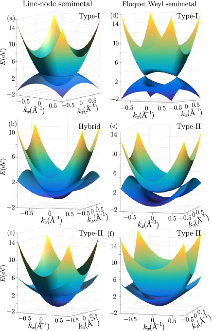
Figure 2: (Color online) (a)-(c) are the energy spectra of undriven type-I, hybrid, and type-II LNSMs with (a) $\left|c_{x}/m_{x}\right|=\left|c_{z}/m_{z}\right|<1$, (b) $\left|c_{x}/m_{x}\right|>1$ and $\left|c_{z}/m_{z}\right|<1$, and (c) $\left|c_{x}/m_{x}\right|=\left|c_{z}/m_{z}\right|>1$, where we take $k_{y}=0$. (d)-(f) are the energy spectra of Floquet WSMs in light-driven type-I, type-II, and hybrid LNSMs along the $x$ axis.

To study the interaction of LNSMs with light, we consider a time-dependent vector potential $\mathbf{A}\left(t\right)=\mathbf{A}\left(t+T\right)$, which is a periodic function with a period of $T=2\pi/\omega$. The driven Hamiltonian $H\left(t\right)$ is obtained by using the Peierls substitution, $\mathbf{k}\rightarrow\mathbf{k}-\mathbf{A}(t)$. In this paper, we focus on the low-energy physics of LNSMs near the nodal ring. Making use of Floquet theoryShirley65PRB ; Sambe73PRA ; Gesztesy81JPMG in the high-frequency limit, the periodically driven system can be described by a static effective Hamiltonian asMaricq82PRB ; Grozdanov88PRB ; Rahav03PRA ; Rahav03PRL ; Goldman14PRX ; Eckardt15NJP ; Bukov15AdvPhys

$$H_{\text{eff}}=H_{0,0}+\frac{\left[H_{0,-1},H_{0,1}\right]}{\hbar\omega}+O\left(A_{L}^{4}\right),$$ (5)

where $\omega$ and $A_{L}$ describe the frequency and amplitude of light, and $H_{m,n}=\frac{1}{T}\int_{0}^{T}H(t)e^{i(m-n)\omega t}dt$ are the discrete Fourier components of the Hamiltonian.

III.1 Light propagating along the $x$ axis

When a light propagates along the $x$ axis, $\mathbf{A}$ is given by $\mathbf{A}=A_{L}\left(0,\cos\omega t,\eta\sin\omega t\right)$, where $\eta=\pm 1$ indicates the chiralities of the circularly polarized light. From Eq. (5), the Floquet correction is

$$\Delta H^{x}=-\frac{A_{L}^{2}}{2}\left(m_{y}+m_{z}\right)\sigma_{z}-Lm_{z}k_{z}\sigma_{x},$$ (6)

with $L=2\eta A_{L}^{2}v_{y}/(\hbar\omega)$. We obtain a term coupling the momentum $k_{z}$ and $\sigma_{x}$, which gaps out the nodal ring except at two Weyl points $\pm\mathbf{k}_{0}=(\pm\sqrt{\tilde{m}_{0}/m_{z}},0,0)$ with $\tilde{m}_{0}=m_{0}-A_{L}^{2}\left(m_{y}+m_{z}\right)/2$. Linearizing the eigenvalues of Hamiltonian around $\mathbf{k}_{0}$, we have the energy dispersion

$$E_{\pm}\left(\mathbf{q}\right) =\frac{2c_{x}\sqrt{\tilde{m}_{0}}}{\sqrt{m_{x}}}q_{x}\pm\sqrt{4\tilde{m}_{0}m_{x}q_{x}^{2}+\left(Lm_{z}q_{z}\right)^{2}+v_{y}^{2}q_{y}^{2}}$$

$$=T(\mathbf{q})\pm U(\mathbf{q}),$$ (7)

where $\mathbf{q}=\mathbf{k}-\mathbf{k}_{0}$. The energy dispersion near $-\mathbf{k}_{0}$ is $E_{\pm}\left(\mathbf{q}\right)=-T(\mathbf{q})\pm U(\mathbf{q})$. The band is tilted along the $x$ axis, and then the tilt ratio of the Weyl points is given by

$$F_{x}=\left|\frac{T\left(q_{x}\right)}{U\left(q_{x}\right)}\right|=\frac{c_{x}}{m_{x}}.$$ (8)

Interestingly, the type of the pair of Weyl nodes only depends on the ratio $c_{x}/m_{x}$ and has nothing to do with the intensity and the frequency of the applied light.

The results above show that when light traveling along the $x$ axis gaps out the nodal ring and leaves a pair of Weyl nodes, the system enters into a WSM phase. However, the type of the Weyl nodes is independent of the intensity and the frequency of the incident light, which implies that a type-II Floquet WSM state arises by driving the type-II LNSM with light along the $x$ axis [Fig. 1(b₃)] since $c_{x}/m_{x}>1$ for the type-II LNSM. For the driven hybrid LNSM, the type of induced Weyl nodes depends on the specific value of $c_{x}/m_{x}$ [Fig. 1(b₂)], that is to say, a type-I WSM state arises if $c_{x}/m_{x}<1$ and a type-II WSM state appears if $c_{x}/m_{x}>1$.

The bulk band spectra of the driven hybrid LNSM with $c_{x}/m_{x}>1$ and the driven type-II LNSM are shown in Figs. 2(e) and 2(f), respectively. It can be seen that the type-II Weyl nodes are separated along the propagation direction of the incident light, as predicted. For comparison, we also plot the band spectrum of the driven type-I LNSM [Fig. 2(d)] showing the type-I Weyl nodes, which were revealed in previous studiesYanZ16PRL ; Narayan16PRB ; Taguchi16PRB1 ; Ezawa17PRB .

III.2 Light propagating along the $y$ axis

When the incident light propagates along the $y$ axis, $\mathbf{A}$ is given by $\mathbf{A}=A_{L}\left(\eta\sin\omega t,0,\cos\omega t\right)$, and it produces the following correction,

$$\Delta H^{y}=-\frac{A_{L}^{2}}{2}\left(m_{x}+m_{z}\right)\sigma_{z}.$$ (9)

The correction term can be absorbed in the second term of Eq. (1) by renormalizing the parameter $m_{0}\rightarrow m_{0}-A_{L}^{2}\left(m_{x}+m_{z}\right)/2$. It means that the incident light propagating along the $y$ axis only shifts the nodal rings instead of gapping them out [Figs. 1(c₁)-1(c₃)].

III.3 Light propagating along the $z$ axis

For light propagating along the $z$ axis, we have $\mathbf{A}=A_{L}\left(\cos\omega t,\eta\sin\omega t,0\right)$. Then the effective Hamiltonian gains additional terms,

$$\Delta H^{z}=-\frac{A_{L}^{2}}{2}\left(m_{x}+m_{y}\right)\sigma_{z}+Lm_{x}k_{x}\sigma_{x}.$$ (10)

In this case, the light gaps out the nodal ring except at two Weyl points $\pm\mathbf{k}_{0}=(0,0,\pm\sqrt{\tilde{m}_{0}^{\prime}/m_{z}})$ with $\tilde{m}_{0}^{\prime}=m_{0}-A_{L}^{2}\left(m_{x}+m_{y}\right)/2$, which is similar to the case of light propagating along the $x$ axis. Linearizing the eigenvalues of Hamiltonian around $\mathbf{k}_{0}$, we have the energy dispersion

$$E_{\pm}\left(\mathbf{q}\right) =\frac{2c_{z}\sqrt{\tilde{m}_{0}^{\prime}}}{\sqrt{m_{z}}}q_{z}\pm\sqrt{4\tilde{m}_{0}^{\prime}m_{z}q_{z}^{2}+\left(Lm_{x}q_{x}\right)^{2}+v_{y}^{2}q_{y}^{2}}$$

$$=T(\mathbf{q})\pm U(\mathbf{q}).$$ (11)

Thus the tilt ratio is

$$F_{z}=\left|\frac{T\left(q_{z}\right)}{U\left(q_{z}\right)}\right|=\frac{c_{z}}{m_{z}}.$$ (12)

We can conclude that, in the presence of light propagating along the $z$ axis, a LNSM evolves into a WSM with a pair of Weyl nodes separated along the propagating direction. The type of Weyl nodes is only determined by the ratio $c_{z}/m_{z}$ [Figs. 1(d₁)-1(d₃)].

III.4 Light propagating on the $x$-$z$ plane

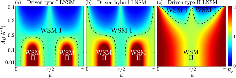
Figure 3: (Color online) Phase diagrams of driven LNSMs in the $(A_{L},\psi)$ phase space. The color bar indicates the tilt ratio $F_{\psi}$. The phase boundaries are marked by the dashed lines, corresponding to $F_{\psi}=1$. The model parameters are taken to be (a) $-c_{x}=c_{y}=c_{z}=3.5\text{ eV \r{A}}^{2}$, (b) $-c_{x}=c_{y}=3.5\text{ eV \r{A}}^{2}$ and $c_{z}=4.5\text{ eV \r{A}}^{2}$, (c) $c_{x}=c_{y}=4.5\text{ eV \r{A}}^{2}$ and $c_{z}=8\text{ eV \r{A}}^{2}$. The common parameters are $m_{x}=m_{y}=m_{z}=4\text{ eV \r{A}}^{2}$, $m_{0}=1\text{ eV}$, $v_{y}=1\text{ eV \r{A}}$, and $\hbar\omega=0.1\text{ eV}$.

We rotate the propagation direction of the incident light on the $x$-$z$ plane with $\mathbf{A}=A_{L}\left(C_{\psi}\cos\omega t,\eta\sin\omega t,-S_{\psi}\cos\omega t\right)$, where $C_{\psi}=\cos\psi$, $S_{\psi}=\sin\psi$, and $\psi$ defines the incident angle off the $z$ axis. When $\psi=0,$ the propagation direction is along the $z$ axis, which is just the case in Sec. III.3. When $\psi=\pi/2,$ the incident direction is along the $x$-axis, which is the case discussed in Sec. III.1. For generic $\psi$, the light induces the following Floquet correction,

$$\Delta H^{xz} =-\frac{A_{L}^{2}}{2}\left(C_{\psi}^{2}m_{x}+m_{y}+S_{\psi}^{2}m_{z}\right)\sigma_{z}$$

$$+L\left(C_{\psi}m_{x}k_{x}-S_{\psi}m_{z}k_{z}\right)\sigma_{x}.$$ (13)

The second term of Eq. (13) is proportional to $\sigma_{x}$, giving rise to a pair of Weyl nodes at

$$\pm\mathbf{k}_{0}=\pm\left(\sqrt{\frac{m_{z}}{m_{x}}}S_{\psi},0,\sqrt{\frac{m_{x}}{m_{z}}}C_{\psi}\right)\sqrt{\frac{\tilde{m}_{0}^{\prime\prime}}{C_{\psi}^{2}m_{x}+S_{\psi}^{2}m_{z}}},$$ (14)

where $\tilde{m}_{0}^{\prime\prime}=m_{0}-A_{L}^{2}\left(C_{\psi}^{2}m_{x}+m_{y}+S_{\psi}^{2}m_{z}\right)/2$. Using the same procedure in Secs. III.1 and III.3, the tilt ratio of the Weyl nodes can be expressed as

$$F_{\psi}=\frac{\lambda_{x}^{2}+\lambda_{z}^{2}}{\sqrt{L^{2}P_{1}^{2}+4m_{x}m_{z}\tilde{m}_{0}^{\prime\prime}P_{2}^{2}/K}},$$ (15)

where $P_{1}=C_{\psi}m_{x}\lambda_{x}-S_{\psi}m_{z}\lambda_{z}$, $P_{2}=S_{\psi}\lambda_{x}+C_{\psi}\lambda_{z}$, and $K=m_{x}C_{\psi}^{2}+m_{z}S_{\psi}^{2}$. We can see that, in this case, the tilt ratio depends on the intensity, frequency, and incident angle of the light, which is quite different from previous cases in which the type of induced Weyl nodes is only determined by the parameters of the original Hamiltonian of LNSMs. This allows us to control the type of Floquet WSMs by tuning the intensity and incident angle of the applied light [Figs. 1(e₁)-1(e₃)]. It implies that we can have a type-I Floquet or a type-II WSM by driving a type-II LNSM with an appropriate light.

Figures 3(a)-3(c) show the phase diagrams in ($A_{L}$, $\psi$) space for driven type-I, hybrid, and type-II LNSMs obtained by monitoring the tilt ratio of the Weyl nodes. The phase diagrams show peculiar features for distinct types of LNSMs. When the light intensity is weak, the driven type-I LNSM [Fig. 3(a)] supports the type-I WSM phase near $\psi=0$, $\pi/2$, and $\pi$, and the type-II WSM phase near $\psi=\pi/4$ and $3\pi/4$. However, for the driven hybrid LNSM, the type-I WSM phase only occupies a small region near $\psi=\pi/2$ in the phase diagram, and the rest of the phase diagram is occupied by the type-II WSM phase [Fig. 3(b)]. This is because we choose a hybrid LNSM with $c_{z}/m_{z}>1$ and $c_{x}/m_{x}<1$. In contrast to the driven type-I and hybrid LNSMs, the driven type-II LNSM hosts only the type-II WSM phase at weak light intensity [Fig. 3(c)]. As the intensity increases, the type-I WSM phase dominates the phase diagrams for all types of driven LNSMs.

Now, we discuss the possibility of an experimental realization of Floquet WSMs in periodically driven LNSMs. Let us consider the realistic parameters $v_{y}=0.6\text{ eV \r{A}}$, $m_{x,y,z}=10\text{ eV \r{A}}^{2}$, and $m_{0}\approx 0.3$ eV for a candidate type-II LNSM material K₄P₃ LiS17PRB . We choose the photon energy to be $\hbar\omega\approx$ 150 meV, which is close to the typical values in recent optical pump-probe experiments. The amplitude of light $A_{L}$ for the onset of a type-I Floquet WSM is about $0.05\text{ \r{A}}^{-1}$, and the corresponding electric field strength $E_{0}=\hbar\omega A_{L}/e$ is $5\times 10^{7}$ V/m, which is within experimental accessibility WangY13Science ; Mahmood16NatPhys , while a type-II WSM phase in the driven system can appear even at very weak light intensity.

IV Photoinduced anomalous hall effect

The photoinduced phase transition from LNSMs to WSMs is accompanied by an anomalous Hall effect since time-reversal breaking WSMs exhibit nonzero, nonquantized Hall conductivity YangKY11PRB ; Burkov14PRL . In this section, we study the photovoltaic anomalous Hall effect of Floquet WSM states in driven LNSMs. We will concentrate on the case in which the incident light propagates along the $x$ axis. The Weyl nodes are located along the $x$-axis, thus the nontrivial component of Hall conductivity is $\sigma_{zy}^{\text{AHE}}$, which can be obtained by use of the Kubo formulaTaguchi16PRB1 ; Oka09PRB

$$\sigma_{zy}^{\text{AHE}} =-i\hbar e^{2}\int\frac{d^{3}\mathbf{k}}{\left(2\pi\right)^{3}}\sum_{\alpha\neq\beta}\frac{f[\epsilon_{F}-E_{\beta}\left(\mathbf{k}\right)]-f[\epsilon_{F}-E_{\alpha}\left(\mathbf{k}\right)]}{E_{\beta}\left(\mathbf{k}\right)-E_{\alpha}\left(\mathbf{k}\right)}$$

$$\times\frac{\left\langle\psi_{\alpha}\left(\mathbf{k}\right)\left|v_{z}\left(\mathbf{k}\right)\right|\psi_{\beta}\left(\mathbf{k}\right)\right\rangle\left\langle\psi_{\beta}\left(\mathbf{k}\right)\left|v_{y}\left(\mathbf{k}\right)\right|\psi_{\alpha}\left(\mathbf{k}\right)\right\rangle}{E_{\beta}\left(\mathbf{k}\right)-E_{\alpha}\left(\mathbf{k}\right)+i\delta},$$ (16)

where $f$ is the Fermi distribution function, $v_{z,y}\left(\mathbf{k}\right)=\left[\partial H\left(\mathbf{k}\right)/\partial k_{z,y}\right]/\hbar$ are the velocity operators along the $z$ and $y$ axes, $\delta$ is an infinitesimal quantity, $E_{\alpha}\left(\mathbf{k}\right)$ is the $\alpha$th band of the effective Hamiltonian, and $\psi_{\alpha}(\mathbf{k})$ is the corresponding eigenvector. The anomalous Hall conductivity is easily obtained when the Fermi energy is located at the Weyl nodes ($\epsilon_{F}=0$) and the temperature is zero. For ideal type-I WSMs, the anomalous Hall conductivity is $\sigma_{\text{type-I}}^{\text{AHE}}=e^{2}Q/(h\pi)$Burkov11PRL ; Burkov11PRB , where $2Q$ is the distance between the Weyl nodes in momentum space. For type-II WSMs, due to the strong tilt of the Weyl nodes, the anomalous Hall conductivity is found to be related to the tilt ratio Zyuzin16JETPL .

For arbitrary Fermi energy $\epsilon_{F}$ and temperature $T$, the anomalous Hall conductivity can be numerically calculated by using Eq. (16). As shown in Fig. 4, we calculate the anomalous Hall conductivity in photoinduced Floquet type-I and type-II WSMs, which correspond to the case shown in Figs. 2(d) and 2(f), respectively. For the Floquet type-I WSM at low temperatures [Fig. 4(a)], the anomalous Hall conductivity reaches its maximum near $\epsilon_{F}=0$, and reduces at finite Fermi energies, whereas for the Floquet type-II WSM at low temperatures [Fig. 4(b)], the maximum value of the anomalous Hall conductivity occurs at a Fermi energy $\epsilon_{F}=-1\text{ eV}$ due to the imbalance between the electron and hole pockets. Note that, the Hall conductivity of the type-I Floquet WSM is asymmetric with respect to the Fermi energy, which is attributed to the weak tilt of the energy dispersion. Because of the anisotropy of the band structure caused by the strong tilt in the energy dispersion, $\sigma_{zy}^{\text{AHE}}$ in the Floquet type-II WSM is highly asymmetric with respect to the Fermi energy.

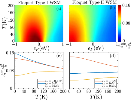
Figure 4: (Color online) The anomalous Hall conductivity $\sigma_{zy}^{\text{AHE}}$ as functions of the Fermi energy $\epsilon_{F}$ and temperature $T$ for (a) the Floquet type-I WSM and (b) the Floquet type-II WSM. The anomalous Hall conductivities $\sigma_{zy}^{\text{AHE}}$ as a function of the temperature $T$ at different Fermi energies $\epsilon_{F}$ for (c) the type-I WSM and (d) the type-II WSM. The common parameters are $m_{x}=m_{y}=m_{z}=4\text{ eV \r{A}}^{2}$, $m_{0}=1\text{ eV}$, $v_{y}=1\text{ eV \r{A}}$, $\hbar\omega=0.1\text{ eV}$, and $A_{L}=0.3\text{ \r{A}}^{-1}$. The parameters for the Floquet type-I WSM are $c_{x}=c_{y}=c_{z}=2\text{ eV \r{A}}^{2}$, and for the Floquet type-II WSM are $c_{x}=c_{y}=c_{z}=8\text{ eV \r{A}}^{2}$.

We plot the anomalous Hall conductivities of the Floquet type-I and type-II WSMs as a function of the temperature $T$ with different Fermi energies in Figs. 4(c) and 4(d). When the Fermi energy is located at the Weyl nodes, i.e., $\epsilon_{F}=0$, the Hall conductivity $\sigma_{zy}^{\text{AHE}}$ for the Floquet type-I WSM decreases with increasing temperature, however, it increases as temperature increases for the Floquet type-II WSM. When the Fermi energy is located below the energy of Weyl nodes, $\epsilon_{F}=-0.5\text{ eV}$ for the type-I Floquet WSM and $\epsilon_{F}=-1\text{ eV}$ for the type-II Floquet WSM, $\sigma_{zy}^{\text{AHE}}$ decreases as the temperature increases. When the Fermi energy is located above the energy of Weyl nodes $\epsilon_{F}=0.5\text{ eV}$, $\sigma_{zy}^{\text{AHE}}$ increases as the temperature increases for both type-I and type-II Floquet WSMs. It is necessary to point out that the results are obtained in the low-temperature regime, and we ignore the high-temperature case where $\sigma_{zy}^{\text{AHE}}$ finally decreases to zero.

V Conclusion

In this paper, we identify a different type of LNSM, a hybrid LNSM, and investigate the effect of off-resonant circularly polarized light on type-II and hybrid LNSMs within the framework of Floquet theory. We show that both of them can support photoinduced Floquet WSM phases. Remarkably, we can manipulate distinct types of WSM states by tuning the incident angle and amplitude of light. Type-II and hybrid LNSMs, along with type-I LNSMs, provide highly controllable platforms for creating WSM states. We also study the anomalous Hall effect of driven LNSMs, which can be used to characterize different types of photoinduced LNSM-WSM transitions.

In comparison with other proposals for realizing artificial WSM phases, such as a magnetically doped topological insulator multilayer Burkov11PRL , driving LNSMs with circularly polarized light is a promising alternative way to realize distinct types of WSM phases without fine tuning, and it does not introduce disorder. The Floquet WSM states in periodically driven LNSMs are ready to be realized, considering the Floquet-Bloch states have been successfully observed on the surface of the topological insulator Bi₂Se₃ by the use of time- and angle-resolved photoemission spectroscopy Mahmood16NatPhys ; WangY13Science . The anomalous Hall effect associated with Floquet WSMs can be detected by transport measurements.

References

- (1) X. Wan, A. M. Turner, A. Vishwanath, and S. Y. Savrasov, Phys. Rev. B 83, 205101 (2011).
- (2) K.-Y. Yang, Y.-M. Lu, and Y. Ran, Phys. Rev. B 84, 075129 (2011).
- (3) S.-M. Huang, S.-Y. Xu, I. Belopolski, C.-C. Lee, G. Chang, B. Wang, N. Alidoust, G. Bian, M. Neupane, C. Zhang, S. Jia, A. Bansil, H. Lin, and M. Z. Hasan, Nat. Commun. 6, 7373 (2015).
- (4) H. Weng, C. Fang, Z. Fang, B. A. Bernevig, and X. Dai, Phys. Rev. X 5, 011029 (2015).
- (5) A. A. Soluyanov, D. Gresch, Z. Wang, Q. Wu, M. Troyer, X. Dai, and B. A. Bernevig, Nature (London) 527, 495 (2015).
- (6) Y. Xu, F. Zhang, and C. Zhang, Phys. Rev. Lett. 115, 265304 (2015).
- (7) F.-Y. Li, X. Luo, X. Dai, Y. Yu, F. Zhang, and G. Chen, Phys. Rev. B 94, 121105(R) (2016).
- (8) S.-Y. Xu, I. Belopolski, N. Alidoust, M. Neupane, G. Bian, C. Zhang, R. Sankar, G. Chang, Z. Yuan, C.-C. Lee, S.-M. Huang, H. Zheng, J. Ma, D. S. Sanchez, B. Wang, A. Bansil, F. Chou, P. P. Shibayev, H. Lin, S. Jia, and M. Z. Hasan, Science 349, 613 (2015).
- (9) B. Q. Lv, H. M. Weng, B. B. Fu, X. P. Wang, H. Miao, J. Ma, P. Richard, X. C. Huang, L. X. Zhao, G. F. Chen, Z. Fang, X. Dai, T. Qian, and H. Ding, Phys. Rev. X 5, 031013 (2015).
- (10) S.-Y. Xu, N. Alidoust, I. Belopolski, Z. Yuan, G. Bian, T.-R. Chang, H. Zheng, V. N. Strocov, D. S. Sanchez, G. Chang, C. Zhang, D. Mou, Y. Wu, L. Huang, C.-C. Lee, S.-M. Huang, B. Wang, A. Bansil, H.-T. Jeng, T. Neupert, A. Kaminski, H. Lin, S. Jia, and M. Z. Hasan, Nat. Phys. 11, 748 (2015).
- (11) L. X. Yang, Z. K. Liu, Y. Sun, H. Peng, H. F. Yang, T. Zhang, B. Zhou, Y. Zhang, Y. F. Guo, M. Rahn, D. Prabhakaran, Z. Hussain, S.-K. Mo, C. Felser, B. Yan, and Y. L. Chen, Nat. Phys. 11, 728 (2015).
- (12) C. Wang, Y. Zhang, J. Huang, S. Nie, G. Liu, A. Liang, Y. Zhang, B. Shen, J. Liu, C. Hu, Y. Ding, D. Liu, Y. Hu, S. He, L. Zhao, L. Yu, J. Hu, J. Wei, Z. Mao, Y. Shi, X. Jia, F. Zhang, S. Zhang, F. Yang, Z. Wang, Q. Peng, H. Weng, X. Dai, Z. Fang, Z. Xu, C. Chen, and X. J. Zhou, Phys. Rev. B 94, 241119(R) (2016).
- (13) F. Y. Bruno, A. Tamai, Q. S. Wu, I. Cucchi, C. Barreteau, A. de la Torre, S. McKeown Walker, S. Riccó, Z. Wang, T. K. Kim, M. Hoesch, M. Shi, N. C. Plumb, E. Giannini, A. A. Soluyanov, and F. Baumberger, Phys. Rev. B 94, 121112(R) (2016).
- (14) Y. Wu, D. Mou, N. H. Jo, K. Sun, L. Huang, S. L. Bud’ko, P. C. Canfield, and A. Kaminski, Phys. Rev. B 94, 121113(R) (2016).
- (15) B. Feng, Y.-H. Chan, Y. Feng, R.-Y. Liu, M.-Y. Chou, K. Kuroda, K. Yaji, A. Harasawa, P. Moras, A. Barinov, W. Malaeb, C. Bareille, T. Kondo, S. Shin, F. Komori, T.-C. Chiang, Y. Shi, and I. Matsuda, Phys. Rev. B 94, 195134 (2016).
- (16) Y. Sun, S.-C. Wu, M. N. Ali, C. Felser, and B. Yan, Phys. Rev. B 92, 161107 (2015).
- (17) Z. Wang, D. Gresch, A. A. Soluyanov, W. Xie, S. Kushwaha, X. Dai, M. Troyer, R. J. Cava, and B. A. Bernevig, Phys. Rev. Lett. 117, 056805 (2016).
- (18) K. Deng, G. Wan, P. Deng, K. Zhang, S. Ding, E. Wang, M. Yan, H. Huang, H. Zhang, Z. Xu, J. Denlinger, A. Fedorov, H. Yang, W. Duan, H. Yao, Y. Wu, S. Fan, H. Zhang, X. Chen, and S. Zhou, Nat. Phys. 12, 1105 (2016).
- (19) L. Huang, T. M. McCormick, M. Ochi, Z. Zhao, M.-T. Suzuki, R. Arita, Y. Wu, D. Mou, H. Cao, J. Yan, N. Trivedi, and A. Kaminski, Nat. Mater. 15, 1155 (2016).
- (20) T. T. Heikkilä and G. E. Volovik, JETP Lett. 93, 59 (2011).
- (21) A. A. Burkov, M. D. Hook, and L. Balents, Phys. Rev. B 84, 235126 (2011).
- (22) C.-K. Chiu, J. C. Y. Teo, A. P. Schnyder, and S. Ryu, Rev. Mod. Phys. 88, 035005 (2016).
- (23) Y.-H. Chan, C.-K. Chiu, M. Y. Chou, and A. P. Schnyder, Phys. Rev. B 93, 205132 (2016).
- (24) C.-K. Chiu and A. P. Schnyder, Phys. Rev. B 90, 205136 (2014).
- (25) C. Fang, Y. Chen, H.-Y. Kee, and L. Fu, Phys. Rev. B 92, 081201(R) (2015).
- (26) M. N. Ali, Q. D. Gibson, T. Klimczuk, and R. J. Cava, Phys. Rev. B 89, 020505 (2014).
- (27) L. S. Xie, L. M. Schoop, E. M. Seibel, Q. D. Gibson, W. Xie, and R. J. Cava, APL Mater. 3, 083602 (2015).
- (28) Y. Kim, B. J. Wieder, C. L. Kane, and A. M. Rappe, Phys. Rev. Lett. 115, 036806 (2015).
- (29) R. Yu, H. Weng, Z. Fang, X. Dai, and X. Hu, Phys. Rev. Lett. 115, 036807 (2015).
- (30) G. Bian, T.-R. Chang, H. Zheng, S. Velury, S.-Y. Xu, T. Neupert, C.-K. Chiu, S.-M. Huang, D. S. Sanchez, I. Belopolski, N. Alidoust, P.-J. Chen, G. Chang, A. Bansil, H.-T. Jeng, H. Lin, and M. Z. Hasan, Phys. Rev. B 93, 121113(R) (2016).
- (31) H. Weng, X. Dai, and Z. Fang, J. Phys. Condens. Matter 28, 303001 (2016).
- (32) H. Huang, J. Liu, D. Vanderbilt, and W. Duan, Phys. Rev. B 93, 201114(R) (2016).
- (33) K. Mullen, B. Uchoa, and D. T. Glatzhofer, Phys. Rev. Lett. 115, 026403 (2015).
- (34) G. Bian, T.-R. Chang, R. Sankar, S.-Y. Xu, H. Zheng, T. Neupert, C.-K. Chiu, S.-M. Huang, G. Chang, I. Belopolski, D. S. Sanchez, M. Neupane, N. Alidoust, C. Liu, B. Wang, C.-C. Lee, H.-T. Jeng, C. Zhang, Z. Yuan, S. Jia, A. Bansil, F. Chou, H. Lin, and M. Z. Hasan, Nat. Commun. 7, 10556 (2016).
- (35) L. M. Schoop, M. N. Ali, C. Straber, A. Topp, A. Varykhalov, D. Marchenko, V. Duppel, S. S. P. Parkin, B. V. Lotsch, and C. R. Ast, Nat. Commun. 7, 11696 (2016).
- (36) M. Neupane, I. Belopolski, M. M. Hosen, D. S. Sanchez, R. Sankar, M. Szlawska, S.-Y. Xu, K. Dimitri, N. Dhakal, P. Maldonado, P. M. Oppeneer, D. Kaczorowski, F. Chou, M. Z. Hasan, and T. Durakiewicz, Phys. Rev. B 93, 201104(R) (2016).
- (37) Y. Wu, L.-L.Wang, E. Mun, D. D. Johnson, D. Mou, L. Huang, Y. Lee, S. L. Bud’ko, P. C. Canfield, and A. Kaminski, Nat. Phys. 12, 667 (2016).
- (38) J. Hu, Z. Tang, J. Liu, X. Liu, Y. Zhu, D. Graf, K. Myhro, S. Tran, C. N. Lau, J. Wei, and Z. Mao, Phys. Rev. Lett. 117, 016602 (2016).
- (39) D. Takane, Z. Wang, S. Souma, K. Nakayama, C. X. Trang, T. Sato, T. Takahashi, and Y. Ando, Phys. Rev. B 94, 121108(R) (2016).
- (40) T. Hyart and T. T. Heikkilä, Phys. Rev. B 93, 235147 (2016).
- (41) G. E. Volovik, and K. Zhang, J. Low Temp. Phys. 189, 276 (2017).
- (42) S. Li, Z.-M. Yu, Y. Liu, S. Guan, S.-S. Wang, X. Zhang, Y. Yao, and S. A. Yang, Phys. Rev. B 96, 081106(R) (2017).
- (43) X. Zhang, L. Jin, X. Dai, and G. Liu, J. Phys. Chem. Lett. 8, 4814 (2017).
- (44) J. He, X. Kong, W. Wang, and S.-P. Kou, arXiv:1709.08287.
- (45) Y. Gao, Y. Chen, Y. Xie, P.-Y. Chang, M. L. Cohen, and S. Zhang, Phys. Rev. B 97, 121108 (2018).
- (46) T.-R. Chang, I. Pletikosic, T. Kong, G. Bian, A. Huang, J. Denlinger, S. K. Kushwaha, B. Sinkovic, H.-T. Jeng, T. Valla, W. Xie, and R. J. Cava, arXiv:1711.09167.
- (47) J.-W. Rhim and Y. B. Kim, Phys. Rev. B 92, 045126 (2015).
- (48) J.-W. Rhim and Y. B. Kim, New. J. Phys. 18, 043010 (2016).
- (49) Z. Yan, P.-W. Huang, and Z. Wang, Phys. Rev. B 93, 085138 (2016).
- (50) S. T. Ramamurthy and T. L. Hughes, Phys. Rev. B 95, 075138 (2017).
- (51) Y. H. Wang, H. Steinberg, P. Jarillo-Herrero, and N. Gedik, Science 342, 453 (2013).
- (52) F. Mahmood, C.-K. Chan, Z. Alpichshev, D. Gardner, Y. Lee, P. A. Lee, and N. Gedik, Nat. Phys. 12, 306 (2016).
- (53) E. J. Sie, J. W. McIver, Y.-H. Lee, L. Fu, J. Kong, and N. Gedik, Nat. Mater. 14, 290 (2015).
- (54) J. Kim, X. Hong, C. Jin, S.-F. Shi, C.-Y. S. Chang, M.-H. Chiu, L.-J. Li, and F. Wang, Science 346, 1205 (2014).
- (55) N. H. Lindner, G. Refael, and V. Galitski, Nat. Phys. 7, 490 (2011).
- (56) P. Titum, N. H. Lindner, and G. Refael, Phys. Rev. B 96, 054207 (2017).
- (57) P. Titum, N. H. Lindner, M. C. Rechtsman, and G. Refael, Phys. Rev. Lett. 114, 056801 (2015).
- (58) T. Oka, and H. Aoki, Phys. Rev. B 79, 081406(R) (2009).
- (59) T. Kitagawa, T. Oka, A. Brataas, L. Fu, and E. Demler, Phys. Rev. B 84, 235108 (2011).
- (60) Z. Gu, H. A. Fertig, D. P. Arovas, and A. Auerbach, Phys. Rev. Lett. 107, 216601 (2011).
- (61) P. M. Perez-Piskunow, G. Usaj, C. A. Balseiro, and L. E. F. Foa Torres, Phys. Rev. B 89, 121401 (2014).
- (62) M. Ezawa, Phys. Rev. Lett. 110, 026603 (2013).
- (63) R. Wang, B. Wang, R. Shen, L. Sheng, and D. Y. Xing, Europhys. Lett. 105, 17004 (2014).
- (64) C.-K. Chan, P. A. Lee, K. S. Burch, J. H. Han, and Y. Ran, Phys. Rev. Lett. 116, 026805 (2016).
- (65) S. Ebihara, K. Fukushima, and T. Oka, Phys. Rev. B 93, 155107 (2016).
- (66) C.-K. Chan, Y.-T. Oh, J. H. Han, and P. A. Lee, Phys. Rev. B 94, 121106(R) (2016).
- (67) Z. Yan and Z. Wang, Phys. Rev. Lett. 117, 087402 (2016).
- (68) A. Narayan, Phys. Rev. B 94, 041409(R) (2016).
- (69) K. Taguchi, D.-H. Xu, A. Yamakage, and K. T. Law, Phys. Rev. B 94, 155206 (2016).
- (70) M. Ezawa, Phys. Rev. B 95, 205201 (2017).
- (71) Z. Yan and Z. Wang, Phys. Rev. B 96, 041206(R) (2017).
- (72) S. Yao, Z. Yan, and Z. Wang, Phys. Rev. B 96, 195303 (2017).
- (73) Z. Yan, R. Bi, H. Shen, L. Lu, S.-C. Zhang, and Z. Wang, Phys. Rev. B 96, 041103(R) (2017).
- (74) J. Klinovaja, P. Stano, and D. Loss, Phys. Rev. Lett. 116, 176401 (2016).
- (75) R. W. Bomantara and J. B. Gong, Phys. Rev. B 94, 235447 (2016); R. W. Bomantara, G. N. Raghava, L. W. Zhou, and J. B. Gong, Phys. Rev. E 93, 022209 (2016).
- (76) C.-K. Chan, N. H. Lindner, G. Refael, and P. A. Lee, Phys. Rev. B 95, 041104 (2017).
- (77) H. Weng, Y. Liang, Q. Xu, R. Yu, Z. Fang, X. Dai, and Y. Kawazoe, Phys. Rev. B 92, 045108 (2015).
- (78) J. H. Shirley, Phys. Rev. 138, B979 (1965).
- (79) H. Sambe, Phys. Rev. A 7, 2203 (1973).
- (80) F. Gesztesy and H. Mitter, J. Phys. A: Math. Gen. 14, L79 (1981).
- (81) M. M. Maricq, Phys. Rev. B 25, 6622 (1982).
- (82) T. P. Grozdanov and M. J. Raković, Phys. Rev. A 38, 1739 (1988).
- (83) S. Rahav, I. Gilary, and S. Fishman, Phys. Rev. A 68, 013820 (2003).
- (84) S. Rahav, I. Gilary, and S. Fishman, Phys. Rev. Lett. 91, 110404 (2003).
- (85) N. Goldman and J. Dalibard, Phys. Rev. X 4, 031027 (2014).
- (86) A. Eckardt and E. Anisimovas, New. J. Phys. 17, 093039 (2015).
- (87) M. Bukov, L. D’Alessio, and A. Polkovnikov, Adv. Phys. 64, 139 (2015).
- (88) A. A. Burkov, Phys. Rev. Lett. 113, 187202 (2014).
- (89) A. A. Burkov and L. Balents, Phys. Rev. Lett. 107, 127205 (2011)
- (90) A. A. Zyuzin and R. P. Tiwari, JETP Lett. 103, 717 (2016).