What breaks parity-time-symmetry? — pseudo-Hermiticity and resonance between positive- and negative-action modes

Abstract

It is generally believed that Parity-Time (PT)-symmetry breaking occurs when eigenvalues or both eigenvalues and eigenvectors coincide. However, we show that this well-accepted picture of PT-symmetry breaking is incorrect. Instead, we demonstrate that the physical mechanism of PT-symmetry breaking is the resonance between positive- and negative-action modes. It is proved that PT-symmetry breaking occurs when and only when this resonance condition is satisfied, and this mechanism applies to all known PT-symmetry breakings observed in different branches of physics. The result is achieved by proving a remarkable fact that in finite dimensions, a PT-symmetric Hamiltonian is necessarily pseudo-Hermitian, regardless whether it is diagonalizable or not.

It is a fundamental assumption of quantum physics that observables are Hermitian operators. Bender and collaborators Bender and Boettcher (1998); Bender et al. (2002); Bender (2007) proposed to relax this assumption by considering Parity-Time (PT)-symmetric operators. Since its conception, PT-symmetry has been found important applications in many branches of physics Jones (1999); Mostafazadeh (2002a); Heiss (2004); Bender (2007); El-Ganainy et al. (2007); Makris et al. (2008, 2010); Schomerus (2010); Chong et al. (2011); Ge et al. (2012); Ramezani et al. (2012), including classical physics Klaiman et al. (2008); Schindler et al. (2011); Peng et al. (2014); Hodaei et al. (2017) and quantum physics Dorey et al. (2007); Musslimani et al. (2008); Longhi (2009); Lin et al. (2011); Szameit et al. (2011); Regensburger et al. (2012); Sarma et al. (2014); Ablowitz and Musslimani (2016); Zhang et al. (2016a); Jahromi et al. (2017). PT-symmetry is also observed in many laboratory experiments Guo et al. (2009); Rüter et al. (2010); Feng et al. (2011); Bittner et al. (2012); Liertzer et al. (2012).

Among all the current research topics actively pursued in the field, the breaking of PT-symmetry is arguably the most prominent one. The question needs to be answered is when and how PT-symmetry breaking occurs as system parameters vary. In this aspect, the role of exceptional points (EPs), which are defined by Kato Kato (1966) to be points in the parameter space where two or more eigenvalues of the system coincide, has been noticed. In most of the existing literature, PT-symmetry breaking is described as the process of two real eigenvalues of the Hamiltonian coinciding on the real axis at EPs and then moving off the real axis in opposite direction to generate a complex conjugate pair of eigenvalues. It is often stated or implied that EPs are the locations for PT-symmetry breaking Brandstetter et al. (2014); Heiss (2004, 2012). Recently, some researchers Klaiman et al. (2008); Ge (2016); Feng et al. (2017); Ashida et al. (2017); El-Ganainy et al. (2018) emphasized that in order to break the PT-symmetry at EPs, the eigenvectors need to coalesce as well. This condition of coalescence of both eigenvalues and eigenvectors is exactly equivalent to the condition that the Hamiltonian $H$ is not diagonalizable at the EPs.

In this paper, we show that these well-known pictures of PT-symmetry breaking are incorrect. To motivate the discussion, we use the following example to show that (i) PT-symmetry breaking occurs at some EPs, but does not at all EPs, and (ii) when PT-symmetry breaking occurs at EPs, the Hamiltonian can be either non-diagonalizable (coalescence of both eigenvalues and eigenvectors) or diagonalizable (coalescence of eigenvalues only). Let’s consider the Hamiltonian

$$H=\left(\begin{array}[]{cccc}-3&c&0&0\\ c&-3&0&0\\ b-ci&7i+a&4-ia&ib\\ -7i+a&b+ic&-ib&4+ia\end{array}\right)\thinspace,$$ (1)

where $a,b$ and $c$ are real numbers. For the parity transformation that switches the first row with the second row, and the third row with the fourth row, $H$ is PT-symmetric. Its eigenvalues are $(-3\pm c,4\pm\sqrt{-a^{2}+b^{2}})$. In the parameter space, EPs locate at $c=0$ and $a=\pm b$, and the corresponding coincident eigenvalues are $-3$ and $4$, respectively. Obviously, PT-symmetry breaking occurs at the EPs with $a=\pm b$. Two of the eigenvalues $(4\pm\sqrt{-a^{2}+b^{2}})$ move towards each other when $b^{2}$ approaches $a^{2}$ from the right on the real axis, and become a complex conjugate pair when $b^{2}$ is less than $a^{2}.$ On the other hand, there is no PT-symmetry breaking at the EPs with $c=0,$ i.e., the eigenvalues $(-3\pm c)$ are always real in the neighborhood of $c=0$ on the real axis.

This example also shows that non-diagonalizable Hamiltonian at EPs (coalescence of both eigenvalues and eigenvectors) is a sufficient but not necessary condition for PT-symmetry breaking. In Fig. 1, the parameter space for $a$ and $b$ is plotted for a fixed $c.$ When $(a,b)$ are in the shaded regions, the eigenvalues $(4\pm\sqrt{-a^{2}+b^{2}})$ are a complex conjugate pair, and when $(a,b)$ are in the un-shaded regions, the eigenvalues $(4\pm\sqrt{-a^{2}+b^{2}})$ are real. The points on the two lines $a=\pm b$ are EPs. It is easy to verify that at the EPs defined by $a=\pm b\neq 0$, $H$ is not diagonalizable. But at the EP $(a=0,b=0)$, $H$ is diagonalizable. When the parameters vary along Path 1 (blue line), PT-symmetry breaking occurs at $EP_{1}$, where $H$ is not diagonalizable. But when the parameters vary along Path 2 (red curve), PT-symmetry breaking occurs at $EP_{2}$, where $H$ is diagonalizable. This shows that PT-symmetry breaking can happen at EPs where the Hamiltonian can be either diagonalizable or non-diagonalizable.

This example will be analyzed in details as Example 1 after the development of our general theory.

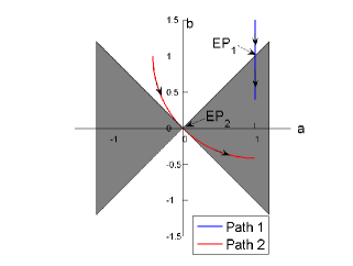
Figure 1: Parameter space for eigenvalues $(4\pm\sqrt{-a^{2}+b^{2}})$ of $H$. In the shaded regions, the eigenvalues are a complex conjugate pair. When the parameters vary along Path 1 (blue line), PT-symmetry breaking occurs at $EP_{1}$, where $H$ is not diagonalizable. But when the parameters vary along Path 2 (red line), there is no PT-symmetry breaking at $EP_{2}$, where $H$ is diagonalizable.

In general, for a finite dimensional system, EP is a necessary but not sufficient condition for PT-symmetry breaking, and EP with coalescence of both eigenvalues and eigenvectors is a sufficient but not a necessary condition. What is a necessary and sufficient condition for PT-symmetry breaking?

In this paper, we will give such a condition. We will first prove a remarkable fact that all PT-symmetric Hamiltonians in the finite dimensions are pseudo-Hermitian Lee and Wich (1969); Mostafazadeh (2002a, b, c). (See Eq. (7) for definition). As a result, an action can be assigned to each eigenmode of a PT-symmetric system. It is shown that if an EP is caused by the resonance between two eigenmodes with the same sign of action, then there is no PT-symmetry breaking at this EP. Otherwise, i.e., if a positive-action mode resonates with a negative-action mode at an EP, then PT-symmetry breaking will occur along a curve passing through this EP in the parameter space. Therefore, resonance between positive- and negative-action modes is a necessary and sufficient condition and thus the physical mechanism for PT-symmetry breaking.

Our result is built upon the mathematical work on the stability of G-Hamiltonian system by Krein, Gel’fand and Lidskii Krein (1950); Gel’fand and Lidskii (1955); Yakubovich and Starzhinskii (1975) in 1950s. It turns out that the definitions of G-Hamiltonian Krein (1950); Gel’fand and Lidskii (1955); Yakubovich and Starzhinskii (1975) and pseudo-Hermitian Lee and Wich (1969); Mostafazadeh (2002a, b, c) are identical for finite dimensions. It is probably more appropriate to adopt the jargon of “G-Hamiltonian”, since it appeared earlier than “pseudo-Hermitian”. However, to be more accessible to the physics community, we will use both. By proving the fact that all finite dimensional PT-symmetric systems are pseudo-Hermitian (or G-Hamiltonian), we are able to borrow the results established by Krein, Gel’fand and Lidskii. Especially, the action we defined for the eigenmodes is the same as the Krein signature for the eigenmodes of G-Hamiltonian systems; and the resonance between positive- and negative-action modes is the same as the well-known Krein collision.

There is another fact that needs to be pointed out. Shortly after the concept of PT-symmetry introduced by Bender et al. Bender and Boettcher (1998), Mostafazadeh proved that a diagonalizable PT-symmetric Hamiltonian is pseudo-Hermitian Mostafazadeh (2002a, b, c). We note that Mostafazadeh’s result is different from ours, which states that a finite dimensional PT-symmetric Hamiltonian is always pseudo-Hermitian, whether it is diagonalizable or not. The difference is significant, because, as we pointed out previously, PT-symmetry breaking occurs at EPs where the Hamiltonian can be either diagonalizable or non-diagonalizable. Apparently, our result is more suitable for the investigation of the the mechanism of PT-symmetry breaking.

We start our investigation from the definitions of PT-symmetry and pseudo-Hermiticity (or G-Hamiltonian property) for the linear system specified by a Hamiltonian $H$,

$$\dot{\bm{x}}=-iH\bm{x}=A\bm{x}\thinspace,$$ (2)

where $A$ is defined to be a shorthand notation of $-iH.$

The Hamiltonian $H$ is called PT-symmetric if

$$PTH-HPT=0\thinspace,$$ (3)

where $P$ is a linear operator satisfying $P^{2}=I$ and $T$ is the complex conjugate operator Bender (2007). In finite dimensions, which will be the focus of the present study, $H$, $A$ and $P$ can be represented by matrices, and the PT-symmetric condition Eq. (3) is equivalent to

$$P\bar{H}-HP=0\textrm{ \thinspace\thinspace or\thinspace\thinspace\ }PA+\bar{A}P=0\thinspace,$$ (4)

Here, $\bar{H}$ and $\bar{A}$ denote the complex conjugates of $H$ and $A$, respectively. The PT-symmetry condition can be understood as follows. In terms of a $P$-reflected variable $\bm{y}\equiv P\bm{x}$, Eq. (2) is

$$\dot{\bm{y}}=PAP^{-1}\bm{y}\thinspace.$$ (5)

In general Eq. (2) is not $P$-symmetric, i.e., $PAP^{-1}\neq A$. However, we can check the effect of applying an additional $T$-reflection, i.e. $t\rightarrow-t$ and $i\rightarrow-i$. Then Eq. (5) becomes

$$\dot{\bar{\bm{y}}}=-\overline{PAP^{-1}}\bar{\bm{y}}\thinspace.$$ (6)

If $-\overline{PAP^{-1}}=A$, which is equivalent to PT-symmetric condition Eq. (3) or Eq. (4), then Eq. (5) in terms of $\bar{\bm{y}}$ is identical to Eq. (2) in terms of $\bm{x}.$ Thus, PT-symmetry is an invariant property of the system under the reflections of both parity and time.

We next define pseudo-Hermiticity or G-Hamiltonian property for the finite-dimensional linear system Eq. (2). A Hamiltonian $H$ is called pseudo-Hermitian if there exist a non-singular Hermitian matrix $G$ and Hermitian matrix $S$ such that

$$H=-G^{-1}S\thinspace;$$ (7)

or equivalently if there exist a non-singular Hermitian matrix $G$ and Hermitian matrix $S$ such that such that $A$ satisfying

$$A=iG^{-1}S\thinspace.$$ (8)

A matrix that can be decomposed as in Eq. (8) is called G-Hamiltonian Yakubovich and Starzhinskii (1975). It is easy to verify that $A$ is G-Hamiltonian or $H$ is pseudo-Hermitian if and only if there exists a non-singular Hermitian matrix $G$ such that

$$A^{*}G+GA=0\thinspace,$$ (9)

where $A^{*}$ is the conjugate transpose of the matrix $A$. As mentioned previously, the concept of G-Hamiltonian was introduced by Krein, Gel’fand and Lidskii Krein (1950); Gel’fand and Lidskii (1955); Yakubovich and Starzhinskii (1975) in 1950s, and pseudo-Hermiticity was introduced by Lee and Wick independently in 1969 Lee and Wich (1969). For finite dimensional systems, the condition for $H$ to be pseudo-Hermitian is identical to that for $A$ to be G-Hamiltonian. We will use both terminologies. Note that the eigenvalues of $A$ are related to those of $H$ by a simple factor of $-i.$

PT-symmetry and pseudo-Hermiticity (or G-Hamiltonian property) are two important geometric or physical properties of the system under investigation. We now establish a connection between PT-symmetry and pseudo-Hermiticity in finite dimensions. First, we give the following necessary and sufficient condition for a matrix to be G-Hamiltonian.

Theorem 1.

For a matrix $A\in C^{n\times n}$, it is G-Hamiltonian if and if only it is similar to $-\bar{A}$, where $\bar{A}$ is its complex conjugate .

Proof.

Necessity is easy to prove. If a matrix is G-Hamiltonian, i.e. satisfying Eq. (9), then $A=-G^{-1}A^{*}G$. Thus matrix $A$ is similar to $-A^{*}$, and also to $-\bar{A}$. We use construction to prove the sufficiency. For a matrix $A\in C^{n\times n}$, it can be written as

$$A=Q^{-1}JQ\thinspace,$$ (10)

where $J$ is its Jordan canonical form and $Q$ is a reversible matrix. It’s well known that its Jordan canonical form consists of several Jordan blocks $J(\lambda)$, where

$$J(\lambda)==\left(\begin{array}[]{cccc}\lambda&1\\ &\ddots&\ddots\\ &&\lambda&1\\ &&&\lambda\end{array}\right)_{m\times m}\thinspace.$$ (11)

When $m=1$, the Jordan block $J(\lambda)$ is reduced to $\lambda$. If $A$ is similar to $-\bar{A}$, then its eigenvalues are symmetric with imaginary axis, and they are either pure imaginary numbers or complex number pairs of the form $\lambda=a+bi$ and $-\bar{\lambda}=-a+bi$, where $a$ and $b$ are real numbers. Accordingly, there are two kinds of matrix blocks

$$F_{1}=J(ia)=\left(\begin{array}[]{cccc}ia&1\\ &\ddots&\ddots\\ &&ia&1\\ &&&ia\end{array}\right)_{m\times m}$$ (12)

and

$$F_{2}=\left(\begin{array}[]{cc}J(a+bi)&0\\ 0&J(-a+bi)\end{array}\right)_{2l\times 2l}.$$ (13)

The Jordan matrix can now be expressed as $J=Diag(M_{1},M_{2},\cdots,M_{k}),$ where $M_{j}$ is in the form of $F_{1}$ or $F_{2}$. In the following, we prove that both types of matrix blocks are G-Hamiltonian. For the first type of matrix block $F_{1}$, if $m$ is odd, the corresponding Hermitian matrix is

$$G=\left(\begin{array}[]{ccccc}&&&&K_{1}\\ &&&K_{1}\\ &&\iddots\\ &K_{1}\\ 1\end{array}\right)\text{,}\thinspace\text{where}\thinspace K_{1}=\left(\begin{array}[]{cc}0&1\\ -1&0\end{array}\right)\thinspace.$$ (14)

For $F_{1}$ with even order and $F_{2}$, the corresponding Hermitian matrix is

$$G=\left(\begin{array}[]{cccc}&&&K_{2}\\ &&K_{2}\\ &\iddots\\ K_{2}\end{array}\right)\thinspace,\text{where}\thinspace K_{2}=\left(\begin{array}[]{cc}0&i\\ -i&0\end{array}\right).$$ (15)

Then for the matrix blocks $M_{j}$, they can be written as $M_{j}=iG_{j}^{-1}S_{j}$. We construct $G^{{}^{\prime}}$ and $S^{{}^{\prime}}$ using $G_{j}$ and $S_{j}$ respectively as follows

$$G^{{}^{\prime}} =Diag(G_{1},G_{2},\cdots,G_{k}),$$ (16)

$$S^{{}^{\prime}} =Diag(S_{1},S_{2},\cdots,S_{k}),$$

and the Jordan canonical form is $J=iG^{{}^{\prime}-1}S^{{}^{\prime}}$. Then we have

$$A=Q^{-1}JQ=Q^{-1}iG^{{}^{\prime}-1}S^{{}^{\prime}}Q=iQ^{-1}G^{{}^{\prime}-1}Q^{-*}Q^{*}S^{{}^{\prime}}Q\thinspace.$$ (17)

Let

$$G =Q^{*}G^{{}^{\prime}}Q$$ (18)

$$S =Q^{*}S^{{}^{\prime}}Q\thinspace,$$ (19)

we obtain

$$A=iG^{-1}S\thinspace,$$ (20)

where $G$ and $S$ are Hermitian matrix, and $G$ is non-singular. ∎

The theorem is proved by constructing a non-singular Hermitian matrix $G$ for a matrix $A$ similar to $-\bar{A}$, but $G$ is not unique. Usually, we can find more than one non-singular Hermitian matrices $G$ for a given matrix $A$.

Because for a PT-symmetric Hamiltonian $H$ satisfying Eq. (4), $A$ is indeed similar to $-\bar{A}$, we have the following important conclusion.

Corollary 2.

For finite dimensional systems, a PT-symmetric Hamiltonian $H$ is also pseudo-Hermitian.

We would like to emphasize again that this fact holds regardless whether $H$ is diagonalizable or not, and some interesting PT-symmetry breaking occurs at EPs where $H$ is not diagonalizable.

The fact that a PT-symmetric system is also pseudo-Hermitian or G-Hamiltonian can be utilized to investigate the mechanism of PT-symmetry breaking. The dynamics of G-Hamiltonian system has been thoroughly developed by Krein, Gel’fand and Lidskii Krein (1950); Gel’fand and Lidskii (1955); Yakubovich and Starzhinskii (1975) in 1950s, and the results can be directly applied to PT-symmetric systems. Specifically, G-Hamiltonian theory gives a comprehensive description on how a stable system becomes unstable as the system varies. In terms of the eigenvalues of the Hamiltonian $H$, this description is about how real eigenvalues of $H$ evolve into conjugate pairs of complex eigenvalues, in another word, how PT-symmetry breaking happens. Let’s briefly summarize the main results of G-Hamiltonian theory. (i) The eigenvalues of a G-Hamiltonian matrix $A$ are symmetric with respect to imaginary axis. They are either pure imaginary numbers or complex pairs. (ii) Let $\psi$ be an eigenmode (or eigenvector) of $A$, an action of $\psi$ can be defined as Zhang et al. (2016b)

$$Ac[\psi]\equiv\left\langle\mathbf{\psi},\psi\right\rangle=\psi^{*}G\psi\thinspace.$$

Mathematically, this is known as the Krein signature Krein (1950); Gel’fand and Lidskii (1955); Yakubovich and Starzhinskii (1975). It is called action because it has the dimension of [energy]$\times$[time]. (ii) The eigenvalues of $A$ can be classified according to the actions of the corresponding eigenvectors. An $r$-fold eigenvalue $\lambda$ ($Re(\lambda)=0$) of $A$ with its eigen-subspace $V_{\lambda}$ is called the first kind if all eigenmodes of $\lambda$ have positive actions, i.e., $Ac[\mathbf{y}]>0$ for any $\mathbf{y}\neq 0$ in $V_{\lambda}$. It is called the second kind if all eigenmodes of $\lambda$ have negative actions. If there exists a zero-action eigenmode, then $\lambda$ is called an eigenvalue of mixed kind Yakubovich and Starzhinskii (1975). If an eigenvalue is the first kind or the second kind, it’s called definite. (iii) The number of each kind of eigenvalue is determined by the Hermitian matrix $G$. Let p be the number of positive eigenvalues and q be the number of negative eigenvalues of the matrix $G$, then any G-Hamiltonian matrix has p eigenvalues of first kind and q eigenvalues of second kind (counting multiplicity). (iv) The G-Hamiltonian matrix is strongly stable if and only if all of its eigenvalues lie on the imaginary axis and are definite. Here, strongly stable means that all eigenvalues of G-Hamiltonian matrix in an open neighborhood of the parameter space lie on the imaginary axis. As a result, a G-Hamiltonian system becomes unstable when and only when a positive-action mode resonates with a negative-action mode. This is a process known as the Krein collision.

Applying these results to PT-symmetric systems, we see that PT-symmetry breaking can happen only when a multiple eigenvalue appears as a result of two eigenmodes resonate, which occurs at an EP. However, if two eigenmodes with the same sign of action resonate at an EP, then there is no PT-symmetry breaking. PT-symmetry breaking is triggered only when a positive-action mode resonates with a negative-action mode. In the following, we use some examples to illustrate these facts.

Example 1: Let’s study in details the PT-symmetry breaking for the PT-symmetric Hamiltonian given by Eq. (1). The associated coefficient matrix $A=-iH$ is G-Hamiltonian with

$$G=\left(\begin{array}[]{cccc}1&i&1&0\\ -i&1&0&1\\ 1&0&0&i\\ 0&1&-i&0\end{array}\right)\thinspace.$$ (21)

This can be directly verified by showing that Eq. (9) is satisfied. The eigenvalues of $G$ are $(\left(3\pm\sqrt{5}\right)/2,\left(-1\pm\sqrt{5}\right)/2)$, three of which are positive and one is negative. Thus, three eigenvalues of $A$ have positive action (or Krein signatures) and the other one has negative action. We calculate the eigenmodes of $A$ numerically and plot the changing process in Fig. 2, where three eigenmodes with positive action are marked by $M_{+}$ and the other one with negative action is marked by $M_{-}$. As shown in Fig. 2(a), we fix $a=1$ and $c=-1$, and vary the parameter $b$ from $2$ to $1/2$. When $b=2$, the eigenvalues of $A$ are all on the imaginary axis. When $b=a=1$, two eigenmodes with different signs of actions resonant on the imaginary axis. As $b$ decreasing the two eigenvalues move off from the imaginary axis and PT-breaking occurs. In Fig. 2(b), we plot the changing process of eigenmodes of $A$ by varying $c$ from $-1$ to $1$ and fixing the other parameters $a=1$ and $b=2$. As $c$ varying, two eigenmodes with opposite signs of actions are locked on the imaginary axis and the other two with positive action move towards each other. When $c=0$, the traveling two eigenmodes collide at the EP. But when increasing $c$ to $1$, they still stay on the imaginary axis and there is no PT-symmetry breaking. These figures demonstrate that at the EP $b=a=1$ where two eigenmodes with different signs of action resonant, PT-symmetry breaking occurs, and at the EP $c=0$ where the collided eigenmodes have the same sign of actions, PT-symmetry breaking does not occur. Meanwhile, we find that at the EPs $b=a=1$, $H$ is not diagonalizable.

On the other hand, we parameterize $a$ and $b$ as $a=1+\sqrt{2}\cos(t)$ and $b=1+\sqrt{2}\sin(t)$, the Hamiltonian becomes

$$H^{{}^{\prime}} =\left(\begin{array}[]{cccc}-3&c&0&0\\ c&-3&0&0\\ 1+\sqrt{2}\sin(t)-ci&7i+1+\sqrt{2}\cos(t)&4-i(1+\sqrt{2}\cos(t))&i(1+\sqrt{2}\sin(t))\\ -7i+1+\sqrt{2}\cos(t)&1+\sqrt{2}\sin(t)+ic&-i(1+\sqrt{2}\sin(t))&4+i(1+\sqrt{2}\cos(t))\end{array}\right).$$ (26)

When varying $t$ form $\pi$ to $3\pi/2$, we obtain the changing process expressed by the red curve in Fig. 1. When $t=5\pi/4$, two eigenmodes with different actions collide on the axis and PT-breaking occurs. The Krein collision process is similar to the process given in Fig. 2(a). At this EP $b=a=0$, $H$ is diagonalizable, i.e., the corresponding eigenvalues resonant, but the eigenvectors don’t.

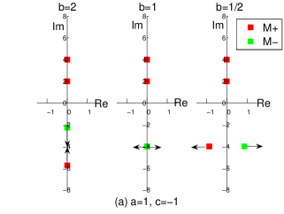
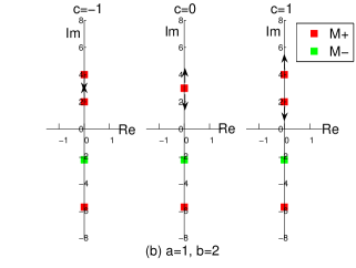
Figure 2: (a) PT-symmetry breaking at the EP when a positive-action eigenmode (red) resonates with a negative eigenmode (green) . (b) No PT-symmetry breaking at the EP when two positive-action eigenmodes (red) resonate.

Example 2: Consider the system of coupled oscillators

$$\ddot{x}+\omega^{2}x+2\gamma\dot{x} =-\varepsilon y\thinspace,$$ (27)

$$\ddot{y}+\omega^{2}y-2\gamma\dot{y} =-\varepsilon x\thinspace,$$ (28)

where $\omega$, $\varepsilon$ and $\gamma$ are real. This is a balanced loss-gain system studied in Bender et al. (2013). Similar and higher dimension examples can be found in refs. Schindler et al. (2011) and Bender et al. (2014), respectively. In terms of canonical coordinate $\bm{x}=(x,y,\dot{x},\dot{y}),$ the system is

$$\dot{\bm{x}} =A\bm{x}$$ (29)

$$A =\left(\begin{array}[]{cccc}0&0&1&0\\ 0&0&0&1\\ -\omega^{2}&-\varepsilon&-2\gamma&0\\ -\varepsilon&-\omega^{2}&0&2\gamma\end{array}\right)\thinspace,$$ (34)

Note that Eq. (29) is a real non-canonical Hamiltonian system. The coefficient matrix $A$ is PT-symmetric, i.e., it satisfies Eq. (4) with

$$P=\left(\begin{array}[]{cccc}0&-1&0&0\\ -1&0&0&0\\ 0&0&0&1\\ 0&0&1&0\end{array}\right)\thinspace.$$ (35)

According to the Corollary 2, $A$ is G-Hamiltonian. We can verify that the following non-singular Hermitian matrix

$$G=\left(\begin{array}[]{cccc}0&-2i\gamma&0&i\\ 2i\gamma&0&i&0\\ 0&-i&0&0\\ -i&0&0&0\end{array}\right)\thinspace$$ (36)

satisfies Eq. (9). The eigenvalues of G in Eq. (36) are $\lambda=\pm\gamma\pm\sqrt{1+\gamma^{2}}$, two of which are positive and the other two are negative. Thus two eigenvalues of $A$ have positive actions (or Krein signatures) and the other two have negative actions. Let’s use numerically calculated examples to observe the breaking of PT-symmetry through the resonance between a positive- and a negative-action mode. We plot the process in Fig. 3 for the case of $\omega=2$ and $\gamma=1$. When $\varepsilon=3.7$, the eigenvalues of $A$ are all imaginary numbers, two of which have positive action (marked by $M_{1+}$ and $M_{2+}$) and the other two have negative action (marked by $M_{1-}$ and $M_{2-}$) in Fig. 3(a). Fig. 3(b) shows that when we decrease $\varepsilon$, $M_{1+}$ and $M_{2-}$ move towards each other, and so do $M_{1-}$ and $M_{2+}$ . Decreasing $\varepsilon$ to $2\sqrt{3}$, eigenmodes $M_{1+}$ and $M_{2-}$ collide on the imaginary axis, and eigenmodes $M_{1-}$ and $M_{2+}$ also collide, as shown in Fig. 3(c). Because the resonance are between modes with different sign of actions, the eigenvalues of $A$ split into pairs symmetric with respect to the imaginary axis and the PT-symmetry is broken. Fig. 3(d) shows that the four eigenvalues of $A$ move out of imaginary axis when $\varepsilon=3.2$. These figures shows that PT-symmetry breaking is triggered at EPs where a positive-actions mode resonates with a negative-action mode. At this EP, $A$ is not diagonalizable.

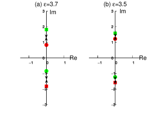
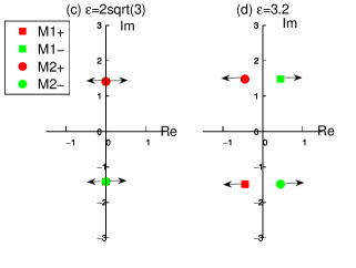
Figure 3: PT-symmetry breaking is triggered at the EP where a positive-actions mode resonates with a negative-action mode. The process is shown for $\omega=2$, $\gamma=1$ and $\varepsilon$ varying from $3.7$ to $3.2$. The EP is at $\varepsilon=2\sqrt{3}$, as shown in (c).

In addition to these two examples, we have verified this mechanism of PT-symmetry breaking for all other PT-symmetric systems that we are aware of.

This research is supported by the National Natural Science Foundation of China (NSFC-11775219, 11775222, 11505186, 11575185 and 11575186), the Fundamental Research Funds for the Central Universities (Grant no. 2017RC033), National Key Research and Development Program (2016YFA0400600, 2016YFA0400601 and 2016YFA0400602), ITER-China Program (2015GB111003, 2014GB124005), the Geo-Algorithmic Plasma Simulator (GAPS) Project, and the U.S. Department of Energy (DE-AC02-09CH11466).

References

- Bender and Boettcher (1998) C. M. Bender and S. Boettcher, Phys. Rev. Lett. 80, 5243 (1998).
- Bender et al. (2002) C. M. Bender, D. C. Brody, and H. F. Jones, Phys. Rev. Lett. 89, 270401 (2002).
- Bender (2007) C. M. Bender, Rep. Prog. Phys. 70, 947 (2007).
- Jones (1999) H. Jones, Phys. Lett. A 262, 242 (1999).
- Mostafazadeh (2002a) A. Mostafazadeh, J. Math. Phys. 43, 205 (2002a).
- Heiss (2004) W. Heiss, J. Phys. A: Math. Gen. 37, 2455 (2004).
- El-Ganainy et al. (2007) R. El-Ganainy, K. Makris, D. Christodoulides, and Z. H. Musslimani, Opt. Lett. 32, 2632 (2007).
- Makris et al. (2008) K. G. Makris, R. El-Ganainy, D. Christodoulides, and Z. H. Musslimani, Phys. Rev. Lett. 100, 103904 (2008).
- Makris et al. (2010) K. G. Makris, R. El-Ganainy, D. N. Christodoulides, and Z. H. Musslimani, Phys. Rev. A 81, 063807 (2010).
- Schomerus (2010) H. Schomerus, Phys. Rev. Lett. 104, 233601 (2010).
- Chong et al. (2011) Y. Chong, L. Ge, and A. D. Stone, Phys. Rev. Lett. 106, 093902 (2011).
- Ge et al. (2012) L. Ge, Y. Chong, and A. D. Stone, Phys. Rev. A 85, 023802 (2012).
- Ramezani et al. (2012) H. Ramezani, T. Kottos, V. Kovanis, and D. N. Christodoulides, Phys. Rev. A 85, 013818 (2012).
- Klaiman et al. (2008) S. Klaiman, U. Günther, and N. Moiseyev, Phys. Rev. Lett. 101, 080402 (2008).
- Schindler et al. (2011) J. Schindler, A. Li, M. C. Zheng, F. M. Ellis, and T. Kottos, Phys. Rev. A 84, 040101 (2011).
- Peng et al. (2014) B. Peng, Ş. K. Özdemir, F. Lei, F. Monifi, M. Gianfreda, G. L. Long, S. Fan, F. Nori, C. M. Bender, and L. Yang, Nat. Phys. 10, 394 (2014).
- Hodaei et al. (2017) H. Hodaei, A. U. Hassan, S. Wittek, H. Garcia-Gracia, R. El-Ganainy, D. N. Christodoulides, and M. Khajavikhan, Nature 548, 187 (2017).
- Dorey et al. (2007) P. Dorey, C. Dunning, and R. Tateo, J. Phys. A: Math. Theor. 40, R205 (2007).
- Musslimani et al. (2008) Z. Musslimani, K. G. Makris, R. El-Ganainy, and D. N. Christodoulides, Phys. Rev. Lett. 100, 030402 (2008).
- Longhi (2009) S. Longhi, Phys. Rev. Lett. 103, 123601 (2009).
- Lin et al. (2011) Z. Lin, H. Ramezani, T. Eichelkraut, T. Kottos, H. Cao, and D. N. Christodoulides, Phys. Rev. Lett. 106, 213901 (2011).
- Szameit et al. (2011) A. Szameit, M. C. Rechtsman, O. Bahat-Treidel, and M. Segev, Phys. Rev. A 84, 021806 (2011).
- Regensburger et al. (2012) A. Regensburger, C. Bersch, M.-A. Miri, G. Onishchukov, D. N. Christodoulides, and U. Peschel, Nature 488, 167 (2012).
- Sarma et al. (2014) A. K. Sarma, M.-A. Miri, Z. H. Musslimani, and D. N. Christodoulides, Phys. Rev. E 89, 052918 (2014).
- Ablowitz and Musslimani (2016) M. J. Ablowitz and Z. H. Musslimani, Nonlinearity 29, 915 (2016).
- Zhang et al. (2016a) Z. Zhang, Y. Zhang, J. Sheng, L. Yang, M.-A. Miri, D. N. Christodoulides, B. He, Y. Zhang, and M. Xiao, Phys. Rev. Lett. 117, 123601 (2016a).
- Jahromi et al. (2017) A. K. Jahromi, A. U. Hassan, D. N. Christodoulides, and A. F. Abouraddy, Nat. Commun. 8, 1359 (2017).
- Guo et al. (2009) A. Guo, G. Salamo, D. Duchesne, R. Morandotti, M. Volatier-Ravat, V. Aimez, G. Siviloglou, and D. Christodoulides, Phys. Rev. Lett. 103, 093902 (2009).
- Rüter et al. (2010) C. E. Rüter, K. G. Makris, R. El-Ganainy, D. N. Christodoulides, M. Segev, and D. Kip, Nat. Phys. 6, 192 (2010).
- Feng et al. (2011) L. Feng, M. Ayache, J. Huang, Y.-L. Xu, M.-H. Lu, Y.-F. Chen, Y. Fainman, and A. Scherer, Science 333, 729 (2011).
- Bittner et al. (2012) S. Bittner, B. Dietz, U. Günther, H. Harney, M. Miski-Oglu, A. Richter, and F. Schäfer, Phys. Rev. Lett. 108, 024101 (2012).
- Liertzer et al. (2012) M. Liertzer, L. Ge, A. Cerjan, A. Stone, H. Türeci, and S. Rotter, Phys. Rev. Lett. 108, 173901 (2012).
- Kato (1966) T. Kato, “Perturbation theory for linear operators,” (Springer-Verlag, Berlin, 1966) p. 64.
- Brandstetter et al. (2014) M. Brandstetter, M. Liertzer, C. Deutsch, P. Klang, J. Schöberl, H. Türeci, G. Strasser, K. Unterrainer, and S. Rotter, Nat. Commun. 5, 4034 (2014).
- Heiss (2012) W. Heiss, J. Phys. A: Math. Theor. 45, 444016 (2012).
- Ge (2016) L. Ge, Phys. Rev. A 94, 013837 (2016).
- Feng et al. (2017) L. Feng, R. El-Ganainy, and L. Ge, Nat. Photonics 11, 752 (2017).
- Ashida et al. (2017) Y. Ashida, S. Furukawa, and M. Ueda, Nat. Commun. 8, 15791 (2017).
- El-Ganainy et al. (2018) R. El-Ganainy, K. G. Makris, M. Khajavikhan, Z. H. Musslimani, S. Rotter, and D. N. Christodoulides, Nat. Phys. 14, 11 (2018).
- Lee and Wich (1969) T. D. Lee and G. C. Wich, Nucl. Phys. B 9, 209 (1969).
- Mostafazadeh (2002b) A. Mostafazadeh, J. Math. Phys. 43, 2814 (2002b).
- Mostafazadeh (2002c) A. Mostafazadeh, J. Math. Phys. 43, 3944 (2002c).
- Krein (1950) M. Krein, Doklady Akad. Nauk. SSSR N.S. 73, 445 (1950).
- Gel’fand and Lidskii (1955) I. M. Gel’fand and V. B. Lidskii, Uspekhi Mat. Nauk 10, 3 (1955).
- Yakubovich and Starzhinskii (1975) V. Yakubovich and V. Starzhinskii, Linear Differential Equations with Periodic Coefficients, Vol. I (Wiley, 1975).
- Zhang et al. (2016b) R. Zhang, H. Qin, R. C. Davidson, J. Liu, and J. Xiao, Phys. Plasmas 23, 072111 (2016b).
- Bender et al. (2013) C. M. Bender, M. Gianfreda, Ş. K. Özdemir, B. Peng, and L. Yang, Phys. Rev. A 88, 062111 (2013).
- Bender et al. (2014) C. M. Bender, M. Gianfreda, and S. Klevansky, Phys. Rev. A 90, 022114 (2014).