On the average condition number of tensor rank decompositions

Abstract.

We compute the expected value of powers of the geometric condition number of random tensor rank decompositions. It is shown in particular that the expected value of the condition number of $n_{1}\times n_{2}\times 2$ tensors with a random rank-$r$ decomposition, given by factor matrices with independent and identically distributed standard normal entries, is infinite. This entails that it is expected and probable that such a rank-$r$ decomposition is sensitive to perturbations of the tensor. Moreover, it provides concrete further evidence that tensor decomposition can be a challenging problem, also from the numerical point of view. On the other hand, we provide strong theoretical and empirical evidence that tensors of size $n_{1}\leavevmode\nobreak\ \times\leavevmode\nobreak\ n_{2}\leavevmode\nobreak\ \times\leavevmode\nobreak\ n_{3}$ with all $n_{1},n_{2},n_{3}\geq 3$ have a finite average condition number. This suggests there exists a gap in the expected sensitivity of tensors between those of format $n_{1}\times n_{2}\times 2$ and other order-3 tensors. For establishing these results, we show that a natural weighted distance from a tensor rank decomposition to the locus of ill-posed decompositions with an infinite geometric condition number is bounded from below by the inverse of this condition number. That is, we prove one inequality towards a so-called condition number theorem for the tensor rank decomposition.

Keywords tensor rank decomposition; CPD; condition number; ill-posed problems; inverse distance to ill-posedness; average complexity;

Subject class Primary 49Q12, 53B20, 15A69; Secondary 14P10, 65F35, 14Q20 49Q12 Sensitivity analysis 53B20 Local Riemannian geometry 15A69 Multilinear algebra, tensor products 14P10 Semialgebraic sets and related spaces 65F35 Matrix norms, conditioning, scaling 14Q20 Effectivity, complexity (computation in AG)

1. Introduction

Whenever data depends on several variables, it may be stored as a $d$-array

$$\mathfrak{A}=\begin{bmatrix}a_{i_{1},i_{2},\ldots,i_{d}}\end{bmatrix}_{i_{1},i_{2},\ldots,i_{d}=1}^{n_{1},n_{2},\ldots,n_{d}}\in\mathbb{R}^{n_{1}\times n_{2}\times\cdots\times n_{d}}.$$

For the purpose of our exposition, this $d$-array is informally called a tensor. Due to the curse of dimensionality, plainly storing this data in a tensor is neither feasible nor insightful. Fortunately, the data of interest often admit additional structure that can be exploited. One particular tensor decomposition is the tensor rank decomposition, or canonical polyadic decomposition (CPD). It was proposed by [32] and expresses a tensor $\mathfrak{A}\in\mathbb{R}^{n_{1}\times n_{2}\times\cdots\times n_{d}}$ as a minimum-length linear combination of rank-$1$ tensors:

(CPD) $$\mathfrak{A}=\mathfrak{A}_{1}+\mathfrak{A}_{2}+\cdots+\mathfrak{A}_{r},\quad\text{where}\quad\mathfrak{A}_{i}=\mathbf{a}_{i}^{1}\otimes\mathbf{a}_{i}^{2}\otimes\cdots\otimes\mathbf{a}_{i}^{d},$$

and where $\otimes$ is the tensor product:

(1.1) $$\mathbf{a}^{1}\otimes\mathbf{a}^{2}\otimes\cdots\otimes\mathbf{a}^{d}=\begin{bmatrix}a_{i_{1}}^{(1)}a_{i_{2}}^{(2)}\cdots a_{i_{d}}^{(d)}\end{bmatrix}_{i_{1},i_{2},\ldots,i_{d}=1}^{n_{1},n_{2},\ldots,n_{d}}\in\mathbb{R}^{n_{1}\times n_{2}\times\cdots\times n_{d}},\quad\text{where $\mathbf{a}^{k}=[a_{i}^{(k)}]_{i=1}^{n_{k}}$.}$$

The smallest $r$ for which the expression CPD is possible is called the rank of $\mathfrak{A}$. In several applications, the CPD of a tensor reveals domain-specific information that is of interest, such as in psychometrics [36], chemical sciences [43], theoretical computer science [11], signal processing [15, 16, 42], statistics [2, 41] and machine learning [3]. In most of these applications, the data that the tensor represents is corrupted by measurement errors, which will cause the CPD computed from the measured data to differ from the CPD of the true, uncorrupted data.

For measuring the sensitivity of a computational problem to perturbations in the data, a standard technique in numerical analysis is investigating the condition number [12, 31]. Earlier theoretical work by the authors introduced two related condition numbers for the computational problem of computing a CPD from a given tensor; see [45, 8]. Let us recall the definition of the geometric condition number of the tensor rank decomposition of [8]. The set of rank-1 tensors $\mathcal{S}\subset\mathbb{R}^{n_{1}\times\cdots\times n_{d}}$ is a smooth manifold, called Segre manifold. The set of tensors of rank at most $r$ is given as the image of the addition map $\Phi:\mathcal{S}^{\times r}\to\mathbb{R}^{n_{1}\times\cdots\times n_{d}},(\mathfrak{A}_{1},\ldots,\mathfrak{A}_{r})\to\mathfrak{A}_{1}+\cdots+\mathfrak{A}_{r}$. The condition number of $\mathfrak{A}$ is defined locally at the decomposition $(\mathfrak{A}_{1},\ldots,\mathfrak{A}_{r})$ as

$$\kappa(\mathfrak{A},(\mathfrak{A}_{1},\ldots,\mathfrak{A}_{r})):=\lim\limits_{\epsilon\to 0}\,\sup\limits_{\mathfrak{B}\text{ has rank }r,\atop\|\mathfrak{A}-\mathfrak{B}\|<\epsilon}\,\frac{\|\Phi^{-1}(\mathfrak{A})-\Phi^{-1}(\mathfrak{B})\|}{\|\mathfrak{A}-\mathfrak{B}\|},$$

where $\Phi^{-1}$ is the local inverse of $\Phi$ with $\Phi^{-1}(\mathfrak{A})={(\mathfrak{A}_{1},\ldots,\mathfrak{A}_{r})}$. If such a local inverse does not exist, we define $\kappa(\mathfrak{A},(\mathfrak{A}_{1},\ldots,\mathfrak{A}_{r})):=+\infty$. The norms are the Euclidean norms induced by the ambient spaces of the domain and image of $\Phi$. As $\mathfrak{A}$ depends uniquely on $(\mathfrak{A}_{1},\ldots,\mathfrak{A}_{r})$ we write $\kappa(\mathfrak{A}_{1},\ldots,\mathfrak{A}_{r})$ for the condition number.

The topic of this paper is the first inquiry into a probabilistic analysis of the condition number of the CPD; see, e.g., [12, 18]. In particular, we focus on the average analysis and compute the expected value of powers of the condition number for random rank-$1$ tuples $(\lambda_{1}\mathfrak{A}_{1},\ldots,\lambda_{r}\mathfrak{A}_{r})$ of length $r$, where the $\lambda_{i}\in\mathbb{R}\setminus\{0\}$ are arbitrary and $\mathfrak{A}_{i}:=\mathbf{a}_{i}^{1}\otimes\cdots\otimes\mathbf{a}_{i}^{d}$ in which the $\mathbf{a}_{i}^{j}\leavevmode\nobreak\ \in\leavevmode\nobreak\ \mathbb{R}^{n_{j}}$ have independently and identically distributed (i.i.d.) standard normal entries. This distribution is very relevant for scientific research, as samples from it are often employed to test the effectiveness of algorithms for computing CPDs. In [8, Proposition 7.1] we have shown that the condition number is invariant under scaling of the rank-one tensors $\mathfrak{A}_{i}$. For this reason, we assume, without loss of generality, that $\lambda_{1}=\cdots=\lambda_{r}=1$ in the remainder of this paper. One of the main results we will prove is the following statement.

Corollary 1.1.

Let $(\mathfrak{A}_{1},\ldots,\mathfrak{A}_{r})\in\mathcal{S}^{\times r}$ be a random rank-$1$ tuple in $\mathbb{R}^{n_{1}\times n_{2}\times n_{3}}$, where $n_{1}\geq n_{2}\geq n_{3}\geq 2$ and $r\geq 2$. Then, we have $\mathbb{E}\,\bigl{[}\kappa(\mathfrak{A}_{1},\ldots,\mathfrak{A}_{r})^{c}\bigr{]}=\infty$, for all $c\geq n_{3}-1$.

In particular, the corollary implies that the expected value of the condition number—without a power—of random rank-$1$ tuples in $\mathbb{R}^{n_{1}\times n_{2}\times 2}$ is $\infty$. This result provides further concrete evidence that the problem of computing a CPD can have a high condition number with a nonnegligible probability. See, for example, the curve $n=2$ in Figure 5.2 which shows the complementary cumulative distribution function of the condition number of random rank-$1$ tuples of length $7$ in $\mathbb{R}^{7\times 7\times 2}$. It shows that there is a $10\%$ chance the condition number is greater than $10^{4}$, and a $1\%$ chance that it is greater than $4\cdot 10^{5}$. In many applications where the CPD is employed, the measurement errors are not sufficiently small to compensate such high condition numbers.

Corollary 1.1 is a contribution to a body of research illustrating that computing CPDs can be a very challenging problem. The result of [34] is often cited in this regard. Håstad reduces 3SAT to computing the rank of a tensor, which shows that the latter problem is NP-complete in the Turing machine computational model. However, this does not entail that computing a typical CPD is a difficult problem. Another oft-cited result by [19] relates to the difficulty of approximating CPDs; they proved that the problem of computing the best rank-$2$ approximation is ill-posed on an open set in $\mathbb{R}^{n_{1}\times n_{2}\times n_{3}}$. Further evidence originates from the sensitivity to perturbations of the CPD: [45] illustrated numerically that the norm-balanced condition number can blow up near the ill-posed locus of [19]; subsequently [8] proved that the geometric condition number will diverge to infinity when approaching the ill-posed locus. Recall from [9, Theorem 1] that the condition number appears in estimates of the rate of convergence and radii of attraction of Riemannian Gauss–Newton methods for computing a best rank-$r$ approximation of a tensor, such as the ones in [9, 10]. Corollary 1.1 thus not only shows that computing CPDs is a difficult problem, but also reinforces the result about the high computational complexity of computing low-rank approximations. Nevertheless, the present article is the first to study average complexity.

There are two new key insights that this paper offers. The first is decidedly negative: the average condition number of random rank-$1$ tuples of length $r$ in $\mathbb{R}^{n_{1}\times n_{2}\times 2}$ is infinite, implying that it is probable to sample a CPD with a high condition number; see Section 5.2. However, the second one is considerably more positive: our inability to reduce the value of $c$ in Corollary 1.1 to $c=1$, or even any value less than $n_{3}-1$, in our analysis, should, in combination with the empirical evidence in Section 5.2 and the impossibility result in Proposition 3.7, be taken as clear evidence for the following conjecture.

Conjecture 1.2.

There exists an integer $2\leq r^{\star}\leq\frac{n_{1}n_{2}n_{3}}{n_{1}+n+2+n_{3}-2}$ such that for all $1\leq r\leq r^{\star}$ and $n_{1}\geq n_{2}\geq n_{3}\geq 3$ the expected condition number of random rank-$1$ tuples of length $r$ in $\mathbb{R}^{n_{1}\times n_{2}\times n_{3}}$ is finite.

This would suggest there exists a gap in sensitivity (which is one measure of complexity, as explained above) between $n_{1}\times n_{2}\times 2$ tensors or pairs of $n_{1}\times n_{2}$ matrices, where the average condition number is proved to be $\infty$, and more general $n_{1}\times n_{2}\times n_{3}$ tensors with $n_{1},n_{2},n_{3}>2$, where all empirical and theoretical evidence points to a finite average condition number. This is similar to the gap in classic complexity between order-$2$ tensors and order-$d$ tensors with $d\geq 3$ for computing the tensor rank. It is noteworthy that increasing the size of the tensor seems to decrease the complexity of computing the CPD.

Statement of the technical contributions

We proved in [8, Theorem 1.3] that the condition number of the CPD is equal to the distance to ill-posedness in an auxiliary space: according to the theorem the condition number of the CPD $\kappa(\mathfrak{A}_{1},\ldots,\mathfrak{A}_{r})$ at a decomposition $(\mathfrak{A}_{1},\ldots,\mathfrak{A}_{r})\in\mathcal{S}^{\times r}$ is equal to the inverse distance of the tuple of tangent spaces $(\mathrm{T}_{\mathfrak{A}_{1}}{\mathcal{S}},\ldots,\mathrm{T}_{\mathfrak{A}_{r}}{\mathcal{S}})$ to ill-posedness:

(1.2) $$\kappa(\mathfrak{A}_{1},\ldots,\mathfrak{A}_{r})=\frac{1}{\mathrm{dist}_{\mathrm{P}}((\mathrm{T}_{\mathfrak{A}_{1}}{\mathcal{S}},\ldots,\mathrm{T}_{\mathfrak{A}_{r}}{\mathcal{S}}),\Sigma_{\mathrm{Gr}})},$$

where $\Sigma_{\mathrm{Gr}}$ and the distance $\mathrm{dist}_{\mathrm{P}}$ are defined as follows. Let $n:=\dim\mathcal{S}$ and write $\Pi:=n_{1}\cdots n_{d}$ for the dimension of $\mathbb{R}^{n_{1}\times\cdots\times n_{d}}$. Denote by $\mathrm{Gr}(\Pi,n)$ the Grassmann manifold of $n$-dimensional linear spaces in the space of tensors $\mathbb{R}^{n_{1}\times\cdots\times n_{d}}\cong\mathbb{R}^{\Pi}$. Then, the tuple of tangent spaces to $\mathcal{S}$ at the decomposition $(\mathfrak{A}_{1},\ldots,\mathfrak{A}_{r})$ is an element in the product of Grassmannians: $(\mathrm{T}_{\mathfrak{A}_{1}}{\mathcal{S}},\ldots,\mathrm{T}_{\mathfrak{A}_{r}}{\mathcal{S}})\in\mathrm{Gr}(\Pi,n)^{\times r}$. The set $\Sigma_{\mathrm{Gr}}$ in 1.2 is then defined as the $r$-tuples of linear spaces that are not in general position. In formulas:

(1.3) $$\Sigma_{\mathrm{Gr}}:=\left\{(W_{1},\ldots,W_{r})\in\mathrm{Gr}(\Pi,n)^{\times r}\mid\dim(W_{1}+\cdots+W_{r})<rn\right\}.$$

The distance measure in 1.2 is the projection distance on $\mathrm{Gr}(\Pi,n)$. It is defined as $\|\mathrm{pr}_{V}-\mathrm{pr}_{W}\|$, where $\mathrm{pr}_{V}$ and $\mathrm{pr}_{W}$ are the orthogonal projections on the spaces $V$ and $W$ respectively, and $\|\cdot\|$ is the spectral norm. This distance is extended to $\mathrm{Gr}(\Pi,n)^{\times r}$ in the usual way:

(1.4) $$\mathrm{dist}_{\mathrm{P}}((V_{1},\ldots,V_{r}),(W_{1},\ldots,W_{r})):=\sqrt{\sum_{i=1}^{r}\|\pi_{V_{i}}-\pi_{W_{i}}\|^{2}}.$$

The decomposition $(\mathfrak{A}_{1},\ldots,\mathfrak{A}_{r})$ whose corresponding tangent space lies in $\Sigma_{\mathrm{Gr}}$ is ill-posed in the following sense. It was shown in [8, Corollary 1.2] that whenever there is a smooth curve $\gamma(t)=(\mathfrak{A}_{1}(t),\ldots,\mathfrak{A}_{r}(t))$ such that $\mathfrak{A}=\sum_{i=1}^{r}\mathfrak{A}_{i}(t)$ is constant, even though $\gamma^{\prime}(0)\leavevmode\nobreak\ \neq\leavevmode\nobreak\ 0$, then all of the decompositions $(\mathfrak{A}_{1}(t),\ldots,\mathfrak{A}_{r}(t))$ of $\mathfrak{A}$ are ill-posed decompositions. Note that in this case, the tensor $\mathfrak{A}$ thus has a family of decompositions running through $(\mathfrak{A}_{1}(0),\ldots,\mathfrak{A}_{r}(0))$. We say that $\mathfrak{A}$ is not locally $r$-identifiable. Tensors are expected to admit only a finite number of decompositions, generically (for the precise statements see, e.g., [1, 13, 6, 14]). Therefore, tensors that are not locally $r$-identifiable are very special as their parameters cannot be identified uniquely. Ill-posed decompositions are exactly those that, using only first-order information, are indistinguishable from decompositions that are not locally $r$-identifiable.

In this article, we relate the condition number to a metric on the data space $\mathcal{S}^{\times r}$; see Theorem 1.3. Following [20], we then use this result and show in Theorem 1.4 that the expected value of the condition number is infinite whenever the ill-posed locus in $\mathcal{S}^{\times r}$ is of codimension 1. To describe the condition number as an inverse distance to ill-posedness on $\mathcal{S}^{\times r}$ we need to consider an angular distance. This is why the main theorem of this article, Theorem 1.3, is naturally stated in projective space.

Theorem 1.3.

Denote by $\pi:\mathbb{R}^{n_{1}\times\cdots\times n_{d}}\backslash\{0\}\to\mathbb{P}(\mathbb{R}^{n_{1}\times\cdots\times n_{d}})$ the canonical projection onto projective space. We put $\mathbb{P}\mathcal{S}:=\pi(\mathcal{S})$ and for tensors $\mathfrak{A}\in\mathbb{R}^{n_{1}\times\cdots\times n_{d}}$ we denote the corresponding class in projective space by $[\mathfrak{A}]:=\pi(\mathfrak{A})$. Let $(\mathfrak{A}_{1},\ldots,\mathfrak{A}_{r})\in\mathcal{S}^{\times r}$. Then,

$$\kappa(\mathfrak{A}_{1},\ldots,\mathfrak{A}_{r})\geq\frac{1}{\mathrm{dist}_{\mathrm{w}}(([\mathfrak{A}_{1}],\ldots,[\mathfrak{A}_{r}]),\Sigma_{\mathbb{P}})},$$

where

$$\Sigma_{\mathbb{P}}=\left\{([\mathfrak{A}_{1}],\ldots,[\mathfrak{A}_{r}])\in(\mathbb{P}\mathcal{S})^{\times r}\mid\kappa(\mathfrak{A}_{1},\ldots,\mathfrak{A}_{r})=\infty\right\}$$

and the distance $\mathrm{dist}_{\mathrm{w}}$ is defined in Definition 2.1.

This characterization of a condition number as an inverse distance to ill-posedness is a called condition number theorem in the literature and it provides a geometric interpretation of complexity of a computational problem. [20] advocates this characterization as it may be used to “compute the probability distribution of the distance from a ‘random’ problem to the set [of ill-posedness].” Condition number theorems were, for instance, derived for matrix inversion [35, 23, 21], polynomial zero finding [33, 21], and computing eigenvalues [46, 21]. For a comprehensive overview see [12, pages 10, 16, 125, 204]. We use the above condition number theorem to derive a result on the average condition number of CPDs.

Theorem 1.4.

Let $(\mathfrak{A}_{1},\ldots,\mathfrak{A}_{r})\in\mathcal{S}^{\times r}$, $r\geq 2$, be a random rank-1 tuple in $\mathbb{R}^{n_{1}\times\cdots\times n_{d}}$. Let $e\geq c\geq 1$. If $\Sigma_{\mathbb{P}}$ contains a manifold of codimension $0$ or $c$ in $\mathcal{S}^{\times r}$, then $\mathbb{E}\,\bigl{[}\kappa(\mathfrak{A}_{1},\ldots,\mathfrak{A}_{r})^{e}\bigr{]}=\infty.$

In Section 3, we prove that for the format $n_{1}\times n_{2}\times n_{3}$, $n_{1}\geq n_{2}\geq n_{3}\geq 2$, the ill-posed locus $\Sigma_{\mathbb{P}}$ contains a submanifold that is of codimension $n_{3}-1$ in $\mathcal{S}^{\times r}$. Hence, the aforementioned Corollary 1.1 is obtained as a consequence of Theorem 1.4.

Remark 1.

The statement of Corollary 1.1 can easily be strengthened as follows. It is known from dimensionality arguments about fibers of projections of projective varieties that there exists an integer critical value $r^{\star}\leq\frac{\dim\mathbb{R}^{n_{1}\times\cdots\times n_{d}}}{\dim\mathcal{S}}$ such that every tensor of rank $r>r^{\star}$ has at least a $1$-dimensional variety of rank decompositions in $\mathcal{S}^{\times r}$; see, e.g., [1, 30, 37]. Specifically, $r^{\star}$ is the smallest value such that the dimension of the projective $(r^{\star}+1)$-secant variety of $\mathbb{P}(\mathcal{S})$ is strictly less than $(r^{\star}+1)\dim\mathcal{S}-1$. It follows then from [8, Corollary 1.2] that the condition number $\kappa(\mathfrak{A}_{1},\ldots,\mathfrak{A}_{r})=\infty$ for all decompositions $(\mathfrak{A}_{1},\ldots,\mathfrak{A}_{r})$ when $r>r^{\star}$. For smaller values of $r$, we can only prove the statement in Corollary 1.1.

Structure of the article

The rest of this paper is structured as follows. In the next section, we recall some preliminary material on Riemannian geometry. We start by proving the main contribution in Section 3, namely Theorem 1.4, because its proof is less technical. Section 4 is devoted to the proof of the condition number theorem, namely Theorem 1.3. In Section 5, we present some numerical experiments and computer algebra computations illustrating the main contributions. Finally, the paper is concluded in Section 6.

Acknowledgements

We thank C. Beltrán for pointing out Lemma 3.2 to us, so that we could use Theorem 1.3 to obtain Theorem 1.4. We like to thank P. Bürgisser for carefully reading through the proof of Proposition 4.3. Anna Seigal is thanked for discussions relating to Lemma 3.6, which she discovered independently. Some parts of this work are also part of the PhD thesis [7] of the first author.

2. Preliminaries and notation

We denote the standard Euclidean inner product on $\mathbb{R}^{m}$ by $\langle\cdot,\cdot\rangle$. The real projective space of dimension $m-1$ is denoted by $\mathbb{P}(\mathbb{R}^{m})$ and the unit sphere of dimension $m-1$ is denoted by $\mathbb{S}(\mathbb{R}^{m})$. Points in linear spaces are typeset in bold-face lower-case symbols like $\mathbf{a},\mathbf{x}$. Points in projective space or other manifolds are typeset in lower-case letters like $a,x$. The orthogonal complement of a point $\mathbf{x}\in\mathbb{R}^{m}$ is $\mathbf{x}^{\perp}:=\{\mathbf{y}\in\mathbb{R}^{m}\mid\langle\mathbf{x},\mathbf{y}\rangle=0\}$. We write $\mathcal{S}$ for the Segre manifold in $\mathbb{R}^{n_{1}\times\cdots\times n_{d}}$. If it is necessary to clarify the parameters, we also write $\mathcal{S}_{n_{1},\ldots,n_{d}}$ . Throughout this paper, $n$ denotes the dimension of $\mathcal{S}$:

(2.1) $$n:=\dim\mathcal{S}_{n_{1},\ldots,n_{d}}=1-d+\sum_{i=1}^{d}n_{i};$$

see [30, 37]. The projective Segre map is

(2.2) $$\sigma:\mathbb{P}(\mathbb{R}^{n_{1}})\times\cdots\times\mathbb{P}(\mathbb{R}^{n_{d}})\to\mathbb{P}\mathcal{S},\;([\mathbf{a}^{1}],\ldots,[\mathbf{a}^{d}])\mapsto[\mathbf{a}^{1}\otimes\cdots\otimes\mathbf{a}^{d}];$$

see [37, Section 4.3.4.].

Let $(M,g)$ be a Riemannian manifold. For $x\in M$ we write $\mathrm{T}_{x}{M}$ for the tangent space of $M$ at $x$. For $\gamma:(-1,1)\to M$ a smooth curve in $M$ we will use the shorthand notations $\gamma^{\prime}(0):=\frac{\mathrm{d}}{\mathrm{d}t}|_{t=0}\gamma(t)$ for the tangent vector in $\mathrm{T}_{\gamma(0)}{M}$ and $\gamma^{\prime}(t):=\frac{\mathrm{d}}{\mathrm{d}t}\gamma(t)$. Recall that the Riemannian distance between two points $p,q\in M$ is $\mathrm{dist}_{M}(p,q)=\inf\left\{l(\gamma)\mid\gamma(0)=p,\gamma(1)=q\right\}$. The infimum is over all piecewise differentiable curves $\gamma:[0,1]\to M$ and the length of a curve is $l(\gamma)=\int_{0}^{1}g(\gamma^{\prime}(t),\gamma^{\prime}(t))^{\frac{1}{2}}\,\mathrm{d}t$. The distance $\mathrm{dist}_{M}$ makes $M$ a metric space [22, Proposition 2.5].

We use the symbol $|\omega|$ to denote the density on $M$ given by $g$ [38, Proposition 16.45]. For densities with finite volume, i.e., $\int_{M}|\omega|<\infty$, this defines the uniform distribution:

$$\operatorname*{\mathrm{Prob}}_{X\text{ uniformly in }M}\{X\in N\}:=\frac{1}{\int_{M}|\omega|}\,\int_{N}|\omega|\quad\text{ where }N\subset M.$$

A particularly important manifold in the context of this article is the projective space $\mathbb{P}(\mathbb{R}^{m})$. An atlas for $\mathbb{P}(\mathbb{R}^{m})$ is, for instance, given by the affine charts $(U_{i},\varphi_{i})$ with $U_{i}=\{(x_{0}:\ldots:x_{m})\mid x_{i}\neq 0\}$ and $\varphi_{i}(x_{0}:\ldots:x_{m})=(\tfrac{x_{0}}{x_{i}},\ldots,\tfrac{x_{i-1}}{x_{i}},\tfrac{x_{i+1}}{x_{i}},\ldots,\tfrac{x_{m}}{x_{i}})$. A Riemannian structure on $\mathbb{P}(\mathbb{R}^{n})$ is the Fubini–Study metric; see, e.g., [12, Section 14.2.2]: the tangent space to $x$ can be identified with

(2.3) $$\mathrm{T}_{x}{\mathbb{P}(\mathbb{R}^{n})\cong\mathbf{x}^{\perp}},\quad\text{ where $\mathbf{x}\in x$ is a representative;}$$

and through this identification the Fubini–Study metric is $g(\mathbf{y}_{1},\mathbf{y}_{2}):=\frac{\langle\mathbf{y}_{1},\mathbf{y}_{2}\rangle}{\|\mathbf{x}\|}$. The Fubini–Study distance $d_{\mathbb{P}}$ is the distance associated to the Fubini–Study metric. For points $x,y\in\mathbb{P}(\mathbb{R}^{n})$ the formula is

$$d_{\mathbb{P}}(x,y)=\frac{|\langle\mathbf{x},\mathbf{y}\rangle|}{\|\mathbf{x}\|\|\mathbf{y}\|},\quad\text{ where $\mathbf{x}\in x$, $\mathbf{y}\in y$ are representatives.}$$

For the Fubini–Study distance in $\mathbb{P}(\mathbb{R}^{n_{1}})\times\cdots\times\mathbb{P}(\mathbb{R}^{n_{d}})$ we write

(2.4) $$\mathrm{dist}_{\mathbb{P}}((x_{1},\ldots,x_{d}),(y_{1},\ldots,y_{d})):=\sqrt{\sum_{i=1}^{d}d_{\mathbb{P}}(x_{i},y_{i})^{2}}.$$

Figure 2.1. The picture depicts relative errors in the weighted distance, where ${x}^{1}\in\mathbb{P}(\mathbb{R}^{n_{1}})$ and ${x}^{2}\in\mathbb{P}(\mathbb{R}^{n_{2}})$ with $n_{1}>n_{2}$. The relative errors of the tangent directions $\Delta{x}^{1}$ and $\Delta{x}^{2}$ are both equal to $\tan\phi$, but the contribution to the weighted distance marked in red is larger for the large circle, which corresponds to the smaller projective space $\mathbb{P}(\mathbb{R}^{n_{2}})$.

The weighted distance, which is the protagonist of Theorem 1.3, is introduced next.

Definition 2.1 (Weighted distance).

The weighted distance between two points $p=(p_{1},\ldots,p_{d})$ and $q=(q_{1},\ldots,q_{d})\in\mathbb{P}(\mathbb{R}^{n_{1}})\times\cdots\times\mathbb{P}(\mathbb{R}^{n_{d}})$ is defined as

$$d_{\mathrm{w}}(p,q):=\sqrt{\sum_{i=1}^{d}(n-n_{i})d_{\mathbb{P}}(p_{i},q_{i})^{2}},$$

where, as before, $n=\dim\mathcal{S}$. The weighted distance on $\mathcal{S}^{\times r}$ then is defined as

$$\mathrm{dist}_{\mathrm{w}}((\mathfrak{A}_{1},\ldots,\mathfrak{A}_{r}),(\mathfrak{B}_{1},\ldots,\mathfrak{B}_{r})):=\sqrt{\sum_{i=1}^{r}d_{\mathrm{w}}(\sigma^{-1}(\mathfrak{A}_{i}),\sigma^{-1}(\mathfrak{B}_{i}))^{2}},$$

where $\sigma^{-1}$ is the inverse of the projective Segre map from 2.2.

For $n_{1}>n_{2}$ the relative errors in the factor $\mathbb{P}(\mathbb{R}^{n_{2}})$ weigh more than relative errors in the factor $\mathbb{P}(\mathbb{R}^{n_{1}})$ when the measure is the weighted distance $d_{\mathrm{w}}$; this is illustrated in Figure 2.1.

3. The expected value of the condition number

Before proving Theorem 1.4, we need four auxiliary lemmata. The first provides a deterministic lower bound of the condition number.

Lemma 3.1.

Let $r\geq 1$. For rank-1 tuples $(\mathfrak{A}_{1},\ldots,\mathfrak{A}_{r})$ in $\mathbb{R}^{n_{1}\times\cdots\times n_{d}}$ we have $\kappa(\mathfrak{A}_{1},\ldots,\mathfrak{A}_{r})\geq 1$.

Proof.

The condition number equals the inverse of the smallest singular value of a matrix all of whose columns are of unit length by [8, Theorem 1.1]. The result follows from the min-max characterization of the smallest singular value. ∎

The next lemma is a basic computation in Riemannian geometry.

Lemma 3.2.

Let $M$ be a Riemannian manifold, and $N$ a codimension $c$ submanifold of $M$. Let $\mathrm{dist}_{M}$ denote the Riemannian distance on $M$ and $|\omega|$ be the density on $M$. Then,

$$\int_{x\in M}\left(\frac{1}{\mathrm{dist}_{M}(x,N)}\right)^{c}\,|\omega|=\infty.$$

Proof.

Let $m,k$ be the dimensions of $M,N$ and let $y\in N$ be any point. Let $\epsilon>0$. From the definition of being a submanifold, there exists an open neighborhood $U$ of $y$ in $M$ and a diffeomorphism $\phi:U\to B_{\epsilon}(\mathbb{R}^{k})\times B_{\epsilon}(\mathbb{R}^{m-k})$, such that $N\cap U=\phi^{-1}(B_{\epsilon}(\mathbb{R}^{k})\times\{0\})$, where $B_{\epsilon}(\mathbb{R}^{m})$ is the open ball of radius $\epsilon$ in $\mathbb{R}^{m}$. By compactness, choosing $\epsilon$ small enough, we can assume that there is a positive constant $C$ such that the derivative of $\phi$ satisfies $\|\mathrm{d}_{x}\phi\|\leq C$, $\|\mathrm{d}_{x}\phi^{-1}\|\leq C$, and $|\det(\mathrm{d}_{x}\phi)|\geq C$ for all $x\in U$. In particular, the length $L$ of a curve in $U$ and the length $L^{\prime}$ of its image under $\phi$ satisfy $L\leq CL^{\prime}$. Writing $(\mathbf{x}_{1},\mathbf{x}_{2}):=\phi(x)$ for the image of $x$ under $\phi$ we thus have $\mathrm{dist}_{M}(x,N)\leq C\|\mathbf{x}_{2}\|.$ The change of variables theorem, i.e., [44, Theorem 3-13], gives

$$\int_{x\in U}\left(\frac{1}{\mathrm{dist}_{M}(x,N)}\right)^{c}\,|\omega| =\int_{x\in U}\left(\frac{1}{\mathrm{dist}_{M}(x,N)}\right)^{m-k}\,|\omega|$$

$$\geq\frac{1}{C^{m-k+1}}\int_{(\mathbf{x}_{1},\mathbf{x}_{2})\in B_{\epsilon}(\mathbb{R}^{k})\times B_{\epsilon}(\mathbb{R}^{m-k})}\frac{1}{\|\mathbf{x}_{2}\|^{m-n}}\,\mathrm{d}\mathbf{x}_{1}\mathrm{d}\mathbf{x}_{2}.$$

Up to positive constants, using Fubini’s theorem, i.e., [44, Theorem 3-10], and passing to polar coordinates, this last integral equals

$$\int_{\mathbf{x}_{1}\in B_{\epsilon}(\mathbb{R}^{k})}\int_{0}^{\epsilon}\frac{t^{m-k-1}}{t^{m-k}}\,\mathrm{d}t\,dv=\infty.$$

The lower bound for the integral in the lemma then follows from

$$\int_{x\in M}\left(\frac{1}{\mathrm{dist}_{M}(x,N)}\right)^{c}\,|\omega|\geq\int_{x\in U}\left(\frac{1}{\mathrm{dist}_{M}(x,N)}\right)^{c}\,|\omega|$$

This finishes the proof. ∎

Inspecting Theorem 1.3, we see that combining it with the above lemma contains the key idea for proving that the expected value of the condition number can be infinite. However, to use these results in our proof of Theorem 1.4, we need to ensure that Lemma 3.2 applies. Theorem 1.3 uses the weighted distance from Definition 2.1 and it is not immediately evident whether it is induced by a Riemannian metric on $\mathbb{P}(\mathbb{R}^{n_{1}})\times\cdots\times\mathbb{P}(\mathbb{R}^{n_{d}})$. Fortunately, the next lemma shows that it is.

Lemma 3.3.

Let $\langle\cdot,\cdot\rangle$ be the Fubini–Study metric. We define the weighted inner product $\langle\cdot,\cdot\rangle_{\mathrm{w}}$ on the tangent space at $p\in\mathbb{P}(\mathbb{R}^{n_{1}})\times\cdots\times\mathbb{P}(\mathbb{R}^{n_{d}})$ as follows. For $\mathbf{u},\mathbf{v}\in\mathrm{T}_{p}{(\mathbb{P}(\mathbb{R}^{n_{1}})\times\cdots\times\mathbb{P}(\mathbb{R}^{n_{d}}))}$, $\mathbf{u}=(\mathbf{u}^{1},\ldots,\mathbf{u}^{d})$, $\mathbf{v}=(\mathbf{v}^{1},\ldots,\mathbf{v}^{d})$, we define $\langle\mathbf{u},\mathbf{v}\rangle_{\mathrm{w}}:=\sum_{i=1}^{d}(n-n_{i})\langle\mathbf{u}^{i},\mathbf{v}^{i}\rangle$. Then, the distance on $\mathbb{P}(\mathbb{R}^{n_{1}})\times\cdots\times\mathbb{P}(\mathbb{R}^{n_{d}})$ corresponding to $\langle\cdot,\cdot\rangle_{\mathrm{w}}$ is $d_{\mathrm{w}}$.

Proof.

Let $\gamma(t)=(\gamma_{1}(t),\ldots,\gamma_{d}(t))$ be a piecewise continuous curve in $\mathbb{P}(\mathbb{R}^{n_{1}})\times\cdots\times\mathbb{P}(\mathbb{R}^{n_{d}})$ connecting $p,q\in\mathbb{P}(\mathbb{R}^{n_{1}})\times\cdots\times\mathbb{P}(\mathbb{R}^{n_{d}})$, such that the distance between $p,q$ given by $\langle\cdot,\cdot\rangle_{\mathrm{w}}$ is

$$\int_{0}^{1}\langle\gamma^{\prime}(t),\gamma^{\prime}(t)\rangle_{\mathrm{w}}^{\frac{1}{2}}\,\mathrm{d}t=\int_{0}^{1}\left(\sum_{i=1}^{d}(n-n_{i})\langle\gamma_{i}^{\prime}(t),\gamma_{i}^{\prime}(t)\rangle\right)^{\frac{1}{2}}\,\mathrm{d}t.$$

Because $(n-n_{i})\langle\gamma_{i}^{\prime}(t),\gamma_{i}^{\prime}(t)\rangle=\langle\sqrt{n-n_{i}}\,\gamma_{i}^{\prime}(t),\sqrt{n-n_{i}}\,\gamma_{i}^{\prime}(t)\rangle$ and because we have the identity of tangent spaces $\mathrm{T}_{\gamma_{i}(t)}{\mathbb{P}(\mathbb{R}^{n_{i}})}=\mathrm{T}_{\gamma_{i}(t)}{\mathbb{S}(\mathbb{R}^{n_{i}})}$ for all $i$ and $t$, we may view $\gamma$ as the shortest path between two points on a product of $d$ spheres with radii $\sqrt{n-n_{1}},\ldots,\sqrt{n-n_{d}}$. The length of this path is $d_{\mathrm{w}}(p,q)$. ∎

Let $\sigma$ be the projective Segre map from 2.2. By [37, Section 4.3.4.], $\sigma$ is a diffeomorphism and we define a Riemannian metric $g$ on $\mathbb{P}\mathcal{S}$ to be the pull-back metric of $\langle\cdot,\cdot\rangle_{\mathrm{w}}$ under $\sigma^{-1}$; see [38, Proposition 13.9]. Then, by construction, we have the following result.

Corollary 3.4.

The weighted distance $\mathrm{dist}_{\mathrm{w}}$ on $\mathbb{P}\mathcal{S}^{\times r}$ is given by the Riemannian metric $g$.

The last technical lemma we need is the following.

Lemma 3.5.

Consider the projective Segre map $\sigma:\mathbb{P}(\mathbb{R}^{n_{1}})\times\cdots\times\mathbb{P}(\mathbb{R}^{n_{d}})\to\mathbb{P}\mathcal{S}$ from 2.2. For any point $p=([\mathbf{a}_{1}],\ldots,[\mathbf{a}_{d}])\in\mathbb{P}(\mathbb{R}^{n_{1}})\times\cdots\times\mathbb{P}(\mathbb{R}^{n_{d}})$ we have $|\det(\mathrm{d}_{p}\sigma)|=1$.

Proof.

We denote by $\mathbf{e}_{i}^{j}$ the $i$th standard basis vector of $\mathbb{R}^{n_{j}}$; i.e., $\mathbf{e}_{i}^{j}$ has zeros everywhere except for the $i$th entry, where it has a 1. To ease notation, let us assume $\mathbf{e}_{i}^{j}$ to be a row vector. Because each $\mathbb{P}(\mathbb{R}^{n_{j}})$ is an orbit of $[\mathbf{e}_{1}^{j}]$ under the orthogonal group, it suffices to show the claim for $p=([\mathbf{e}_{1}^{1}],\ldots,[\mathbf{e}_{1}^{d}])$. By 2.3, an orthonormal basis for the tangent space $\mathrm{T}_{[\mathbf{e}_{1}^{j}]}{\mathbb{P}(\mathbb{R}^{n_{j}})}$ is $\{\mathbf{e}_{2}^{j},\ldots,\mathbf{e}_{n_{j}}^{j}\}$. Hence, an orthonormal basis for $\mathrm{T}_{p}{(\mathbb{P}(\mathbb{R}^{n_{1}})\times\cdots\times\mathbb{P}(\mathbb{R}^{n_{d}}))}$ is

$$\bigcup_{j=1}^{d}\{(\underbrace{0,\ldots,0}_{j-1\text{ times}},\mathbf{e}_{i}^{j},\underbrace{0,\ldots,0}_{d-j+1\text{ times}})\mid 2\leq i\leq n_{j}\}.$$

Fix $1\leq j\leq d$ and $2\leq i\leq n_{j}$. Then, by the product rule, we have

$$\mathrm{d}_{p}\sigma(0,\ldots,0,\mathbf{e}_{j},0,\ldots,0)=\mathbf{e}_{1}^{1}\otimes\cdots\otimes\mathbf{e}_{1}^{j-1}\otimes\mathbf{e}_{i}^{j}\otimes\mathbf{e}_{1}^{j+1}\otimes\cdots\otimes\mathbf{e}_{1}^{d}.$$

It is easily verified that $\{\mathbf{e}_{1}^{1}\otimes\cdots\otimes\mathbf{e}_{1}^{j-1}\otimes\mathbf{e}_{i}^{j}\otimes\mathbf{e}_{1}^{j+1}\otimes\cdots\otimes\mathbf{e}_{1}^{d}\mid 1\leq j\leq d,2\leq i\leq n_{j}\}$ is an orthonormal basis of $\mathrm{T}_{\sigma(p)}{\mathbb{P}\mathcal{S}}$ (for instance, by using Lemma A.1 below). This shows that $\mathrm{d}_{p}\sigma$ maps an orthonormal basis to an orthonormal basis. Hence, $|\det(\mathrm{d}_{p}\sigma)|=1$. ∎

Remark 2.

In fact, the proof of the foregoing lemma shows more than $|\det(\mathrm{d}_{p}\sigma)|=1$. Namely, it shows that $\sigma$ is an isomety in the sense of Definition 4.1.

Now we have gathered all the ingredients to prove Theorem 1.4.

Proof of Theorem 1.4.

First, we use that the condition number is scale invariant. That is, for all $t_{1},\ldots,t_{r}\in\mathbb{R}\backslash\{0\}$ we have by [8, Proposition 4.4]:

$$\kappa(t_{1}\mathfrak{A}_{1},\ldots,t_{r}\mathfrak{A})=\kappa(\mathfrak{A}_{1},\ldots,\mathfrak{A}).$$

This implies that the random variable under consideration is independent of the scaling of the factors $\mathbf{a}_{i}^{j}$ and, consequently, we have (see, e.g., [12, Remark 2.24])

$$\operatorname*{\mathbb{E}}\limits_{\mathbf{a}_{i}^{j}\in\mathbb{R}^{m_{j}},1\leq j\leq d,1\leq i\leq r\atop\text{ standard normal i.i.d.}}\,\bigl{[}\kappa(\mathfrak{A}_{1},\ldots,\mathfrak{A}_{r})^{c}\bigr{]}=\operatorname*{\mathbb{E}}\limits_{\mathbf{a}_{i}^{j}\in\mathbb{P}(\mathbb{R}^{m_{j}}),1\leq j\leq d,1\leq i\leq r\atop\text{ uniformly i.i.d.}}\,\bigl{[}\kappa(\mathfrak{A}_{1},\ldots,\mathfrak{A}_{r})^{c}\bigr{]}.$$

Let $|\omega|$ denote the density on $\mathcal{S}^{\times r}=\mathcal{S}_{n_{1},\ldots,n_{d}}^{\times r}$. By Lemma 3.5, the Jacobian of the change of variables via the projective Segre map $\sigma$ is constant and equal to 1. Hence,

$$\operatorname*{\mathbb{E}}\limits_{\mathbf{a}_{i}^{j}\in\mathbb{P}(\mathbb{R}^{m_{j}}),1\leq j\leq d,1\leq i\leq r\atop\text{ uniformly i.i.d.}}\,\bigl{[}\kappa(\mathfrak{A}_{1},\ldots,\mathfrak{A}_{r})^{c}\bigr{]}=\frac{1}{C}\int_{(\mathfrak{A}_{1},\ldots,\mathfrak{A}_{r})\in\mathbb{P}\mathcal{S}^{\times r}}\kappa(\mathfrak{A}_{1},\ldots,\mathfrak{A}_{r})^{c}\,|\omega|,$$

where $C=\int_{\mathbb{P}\mathcal{S}^{\times r}}|\omega|<\infty$, because $\mathbb{P}\mathcal{S}^{\times r}$ is compact. For brevity, we write $\mathfrak{p}=(\mathfrak{A}_{1},\ldots,\mathfrak{A}_{r})$. Then, by Theorem 1.3 we have

$$\int_{\mathfrak{p}\in\mathbb{P}\mathcal{S}^{\times r}}\kappa(\mathfrak{p})^{c}\,|\omega|\geq\int_{\mathfrak{p}\in\mathbb{P}\mathcal{S}^{\times r}}\left(\frac{1}{\mathrm{dist}_{\mathrm{w}}(\mathfrak{p},\Sigma_{\mathbb{P}})}\right)^{c}\,|\omega|.$$

We cannot directly apply Lemma 3.6 here, because the weighted distance $\mathrm{dist}_{\mathrm{w}}$ is not given by the product Fubini–Study metric. However, from the definitions of the weighted distance and the Fubini–Study distance 2.4, we find $\mathrm{dist}_{\mathrm{w}}(\mathfrak{p},\Sigma_{\mathbb{P}})\leq\sqrt{n}\,\mathrm{dist}_{\mathbb{P}}(\mathfrak{p},\Sigma_{\mathbb{P}}))$. Therefore, we have

$$\int_{\mathfrak{p}\in\mathbb{P}\mathcal{S}^{\times r}}\left(\frac{1}{\mathrm{dist}_{\mathrm{w}}(\mathfrak{p},\Sigma_{\mathbb{P}})}\right)^{c}\,|\omega|\geq n^{-\frac{c}{2}}\int_{\mathfrak{p}\in\mathbb{P}\mathcal{S}^{\times r}}\left(\frac{1}{\mathrm{dist}_{\mathbb{P}}(\mathfrak{p},\Sigma_{\mathbb{P}})}\right)^{c}\,|\omega|.$$

By assumption, there is a manifold $U\subset\Sigma_{\mathbb{P}}$ of codimension $c$ in $\mathcal{S}^{\times r}$ Applying Lemma 3.2 to this manifold we have

$$\int_{\mathfrak{A}_{1},\ldots,\mathfrak{A}_{r}\in\mathbb{P}\mathcal{S}}\left(\frac{1}{\mathrm{dist}_{\mathbb{P}}((\mathfrak{A}_{1},\ldots,\mathfrak{A}_{r}),\Sigma_{\mathbb{P}})}\right)^{c}\,|\omega|\geq\int_{\mathfrak{A}_{1},\ldots,\mathfrak{A}_{r}\in\mathbb{P}\mathcal{S}}\left(\frac{1}{\mathrm{dist}_{\mathbb{P}}((\mathfrak{A}_{1},\ldots,\mathfrak{A}_{r}),U)}\right)^{c}\,|\omega|=\infty.$$

Putting all the equalities and inequalities together, we therefore get

$$\operatorname*{\mathbb{E}}\limits_{\mathbf{a}_{i}^{j}\in\mathbb{R}^{m_{j}},1\leq j\leq d,1\leq i\leq r\atop\text{ standard normal i.i.d.}}\,\bigl{[}\kappa(\mathfrak{A}_{1},\ldots,\mathfrak{A}_{r})^{c}\bigr{]}=\infty.$$

By Lemma 3.1, the condition number satisfies $\kappa(\mathfrak{A}_{1},\ldots,\mathfrak{A}_{r})\geq 1$ for every $(\mathfrak{A}_{1},\ldots,\mathfrak{A}_{r})\in\mathcal{S}^{\times r}$. This together with the foregoing equation implies for $c\leq e$:

$$\operatorname*{\mathbb{E}}\limits_{\mathbf{a}_{i}^{j}\in\mathbb{R}^{m_{j}},1\leq j\leq d,1\leq i\leq r\atop\text{ standard normal i.i.d.}}\,\bigl{[}\kappa(\mathfrak{A}_{1},\ldots,\mathfrak{A}_{r})^{e}\bigr{]}=\infty.$$

The proof is finished. ∎

Next, we investigate a particular corollary of the foregoing result. We will show that for third-order tensors $\mathbb{R}^{n_{1}\times n_{2}\times n_{3}}$, $n_{1}\geq n_{2}\geq n_{3}\geq 2$, the expected value of $(n_{3}-1)$th power of the condition number of random rank-$r$ tensors is indeed $\infty$. The following is the key ingredient.

Lemma 3.6.

Let $\mathcal{S}$ be the Segre manifold in $\mathbb{R}^{n_{1}\times n_{2}\times n_{3}}$, $n_{1}\geq n_{2}\geq n_{3}\geq 2$, and let $\Sigma_{\mathbb{P}}\subset(\mathbb{P}\mathcal{S})^{\times r}$ be the ill-posed locus. Then, there is a subvariety $\mathcal{V}\subset\Sigma_{\mathbb{P}}$ of codimension $n_{3}-1$ in $(\mathbb{P}\mathcal{S})^{\times r}$.

Proof.

Consider the regular map

$$\psi:\left(\mathbb{P}(\mathbb{R}^{n_{1}})\times\mathbb{P}(\mathbb{R}^{n_{2}})\times\mathbb{P}(\mathbb{R}^{n_{3}}))^{\times r-1}\times\mathbb{P}(\mathbb{R}^{n_{1}}\right)\times\mathbb{P}(\mathbb{R}^{n_{2}}) \to(\mathbb{P}\mathcal{S})^{\times r}$$

$$\bigl{(}([\mathbf{a}_{i}],[\mathbf{b}_{i}],[\mathbf{c}_{i}])_{i=1}^{r-1},([\mathbf{a}_{r}],[\mathbf{b}_{r}])\bigr{)} \mapsto\bigl{(}([\mathbf{a}_{i}\otimes\mathbf{b}_{i}\otimes\mathbf{c}_{i}])_{i=1}^{r-1},[\mathbf{a}_{r}\otimes\mathbf{b}_{r}\otimes\mathbf{c}_{1}]\bigr{)}.$$

The image of $\psi$, write $\mathcal{V}=\operatorname{Im}(\psi)$, is a projective variety by [30, Theorem 3.13]. Because the projective Segre map from 2.2 is a bijection, the fiber of $\psi$ at any point in $\mathcal{V}$ consists of precisely one point. As a result, by [30, Theorem 11.12], $\dim\mathcal{V}$ equals the dimension of the source, which is seen to be $r(\dim\mathbb{P}\mathcal{S})-n_{3}+1$, i.e., $\operatorname{codim}(\mathcal{V})=n_{3}-1$.

Next, we show that $\mathcal{V}\subset\Sigma_{\mathbb{P}}$, which then concludes the proof. Let $[\mathfrak{A}_{i}]=[\mathbf{a}_{i}\otimes\mathbf{b}_{i}\otimes\mathbf{c}_{i}]$ be such that $([\mathfrak{A}_{1}],\ldots,[\mathfrak{A}_{r}])\in\mathcal{V}$. Thus, $[\mathbf{c}_{r}]=[\mathbf{c}_{1}]$. Consider the (affine) tangent spaces

$$\mathrm{T}_{\mathfrak{A}_{1}}{\mathcal{S}}=\mathrm{T}_{\mathbf{a}_{1}\otimes\mathbf{b}_{1}\otimes\mathbf{c}_{1}}{\mathcal{S}} =\mathbb{R}^{n_{1}}\otimes\mathbf{b}_{1}\otimes\mathbf{c}_{1}+\mathbf{a}_{1}\otimes(\mathbf{b}_{1})^{\perp}\otimes\mathbf{c}_{1}+\mathbf{a}_{1}\otimes\mathbf{b}_{1}\otimes(\mathbf{c}_{1})^{\perp},\text{ and }$$

$$\mathrm{T}_{\mathfrak{A}_{r}}{\mathcal{S}}=\mathrm{T}_{\mathbf{a}_{r}\otimes\mathbf{b}_{r}\otimes\mathbf{c}_{1}}{\mathcal{S}} =(\mathbf{a}_{r})^{\perp}\otimes\mathbf{b}_{r}\otimes\mathbf{c}_{1}+\mathbf{a}_{r}\otimes\mathbb{R}^{n_{2}}\otimes\mathbf{c}_{1}+\mathbf{a}_{r}\otimes\mathbf{b}_{r}\otimes(\mathbf{c}_{1})^{\perp}.$$

They intersect at least in the $1$-dimensional subspace $\{\alpha\,\mathbf{a}_{r}\otimes\mathbf{b}_{1}\otimes\mathbf{c}_{1}\mid\alpha\in\mathbb{R}\}$. This means that

$$\mathrm{dist}_{\mathrm{P}}((\mathrm{T}_{\mathfrak{A}_{1}}{\mathcal{S}},\ldots,\mathrm{T}_{\mathfrak{A}_{r}}{\mathcal{S}}),\Sigma_{\mathrm{Gr}})=0;$$

hence, by 1.2, $\kappa(\mathfrak{A}_{1},\ldots,\mathfrak{A}_{r})=\infty$ and so $([\mathfrak{A}_{1}],\ldots,[\mathfrak{A}_{r}])\in\Sigma_{\mathbb{P}}$. ∎

We can now wrap up the proof of Corollary 1.1.

Proof of Corollary 1.1.

Lemma 3.6 shows there is a subvariety $\mathcal{V}\subset\Sigma_{\mathbb{P}}$ with codimension equal to $n_{3}-1$. Let $p$ be any smooth point in this subvariety, and consider a neighborhood $U$ of $p$ in $(\mathbb{P}\mathcal{S})^{\times r}$ such that all points in $U$ are smooth points of $\mathcal{V}$. Then, $U$ is a submanifold of $\Sigma_{\mathbb{P}}$ that has codimension $n_{3}-1$ in $\mathcal{S}^{\times r}$. Hence, Theorem 1.4 applies and Corollary 1.1 is proven. ∎

Lemma 3.6 still leaves some doubt over the precise codimension of $\Sigma_{\mathbb{P}}$ in other tensor formats than $n_{1}\times n_{2}\times 2$. It might be possible to sharpen Corollary 1.1. Namely, if there exists a submanifold $\mathcal{M}$ of codimension $k<n_{3}-1$ in $(\mathbb{P}\mathcal{S})^{\times r}$ with $\mathcal{M}\subset\Sigma_{\mathbb{P}}$, then we also have $\mathbb{E}[\kappa(\mathfrak{A}_{1},\ldots,\mathfrak{A}_{r})^{k}]=\infty$. For small tensors, we can compute the codimension of the ill-posed locus using computer algebra software. Employing Macaulay2 [26], we were able to show that Lemma 3.6 cannot be improved for small tensors with rank $r=2$.

Proposition 3.7.

Let $\mathcal{S}$ be the Segre manifold in $\mathbb{R}^{n_{1}\times n_{2}\times n_{3}}$, $10\geq n_{1}\geq n_{2}\geq n_{3}\geq 2$, and let $\Sigma_{\mathbb{P}}\subset(\mathbb{P}\mathcal{S})^{\times 2}$ be the ill-posed locus. There is no subvariety $\mathcal{V}\subset\Sigma_{\mathbb{P}}$ of codimension $k<n_{3}-1$.

Proof.

It is an exercise to verify that the Segre manifold $\mathcal{S}$ is covered by the charts $(U_{i,j},\phi_{i,j})$, defined uniquely as follows: $U_{i,j}:=\operatorname{Im}(\phi_{i,j}^{-1})$ and

$$\phi_{i,j}:\, \mathbb{R}^{n_{1}-1}\times\mathbb{R}^{n_{2}-1}\times\mathbb{R}^{n_{3}}\to\mathbb{R}^{n_{1}\times n_{2}\times n_{3}},$$

$$(\mathbf{x},\mathbf{y},\mathbf{z})\mapsto(x_{1},\ldots,x_{i-1},1,x_{i+1},\ldots,x_{n_{1}-1})\otimes(y_{1},\ldots,y_{j-1},1,y_{j+1},\ldots,y_{n_{2}-1})\otimes\mathbf{z}.$$

Let $p_{1}\in U_{i_{1},j_{1}}$ and $p_{2}\in U_{i_{2},j_{2}}$ and $\mathfrak{A}_{1}=\phi_{i_{1},j_{1}}(p_{1})$, $\mathfrak{A}_{2}=\phi_{i_{2},j_{2}}(p_{2})$. The corresponding rank-2 tensor is $\Phi(\mathfrak{A}_{1},\mathfrak{A}_{2})=\mathfrak{A}_{1}+\mathfrak{A}_{2}$. By definition of the derivative of the addition map $\Phi$, its matrix with respect to an orthonormal basis for $\phi_{i_{1},j_{1}}(U_{i_{1},j_{1}})\times\phi_{i_{2},j_{2}}(U_{i_{2},j_{2}})$ and the standard basis on $\mathbb{R}^{n_{1}\times n_{2}\times n_{3}}\simeq\mathbb{R}^{n_{1}n_{2}n_{3}}$ is the Jacobian of the transformation $\Phi\circ(\phi_{i_{1},j_{1}}\times\phi_{i_{2},j_{2}})$; see [38, pages 55–65]. For example, if $i_{1}=j_{1}=i_{2}=j_{2}$ and $n_{1}=n_{2}=n_{3}=2$, then the derivative $\mathrm{d}_{(\mathfrak{A}_{1},\mathfrak{A}_{2})}\Phi$ is represented in bases as the $8\times 8$ Jacobian matrix of the map from $(\mathbb{R}^{1}\times\mathbb{R}^{1}\times\mathbb{R}^{2})\times(\mathbb{R}^{1}\times\mathbb{R}^{1}\times\mathbb{R}^{2})\to\mathbb{R}^{8}$ taking

$$(a_{2},b_{2},c_{1},c_{2})\times(x_{2},y_{2},z_{1},z_{2})\mapsto\begin{bmatrix}1\\ a_{2}\end{bmatrix}\otimes\begin{bmatrix}1\\ b_{2}\end{bmatrix}\otimes\begin{bmatrix}c_{1}\\ c_{2}\end{bmatrix}+\begin{bmatrix}1\\ x_{2}\end{bmatrix}\otimes\begin{bmatrix}1\\ y_{2}\end{bmatrix}\otimes\begin{bmatrix}z_{1}\\ z_{2}\end{bmatrix}.$$

The ill-posed locus is then the projectivization of the locus where these Jacobian matrices have linearly dependent columns. Note that the codimension of $\Sigma_{\mathbb{P}}\in(\mathbb{P}\mathcal{S})^{\times 2}$ is the same as the codimension in $\mathcal{S}^{\times 2}$ of the affine cone over $\Sigma_{\mathbb{P}}$. The codimension of the variety where these Jacobian matrices are not injective is the number we need to compute. This variety is given by the vanishing of all maximal minors.

Let $s=n_{1}+n_{2}+n_{3}-2=\dim\mathcal{S}$. Computing all $\binom{n_{1}n_{2}n_{3}}{2s}$ maximal minors of a Jacobian matrix $J$ is too expensive. Instead we proceed as follows. Note that we can perform all computations over $\mathbb{Q}$, because the Jacobian matrix is given by polynomials with integer coefficients. By homogeneity, we can always assume that the first rank-$1$ tensor is $p_{1}=\mathbf{e}_{1}^{1}\otimes\mathbf{e}_{1}^{2}\otimes\mathbf{e}_{1}^{3}\in\mathcal{S}$, where $\mathbf{e}_{1}^{j}\in\mathbb{Q}^{n_{j}}$ is the first standard basis vector. For each chart on the second copy of $\mathcal{S}$, we then take $p_{2}\in U_{i_{2},j_{2}}$ and construct the Jacobian matrix $J$. We then multiply it with the column vector $\mathbf{k}=(k_{1},k_{2},\ldots,k_{s})\in\mathbb{Q}^{s}\setminus\{0\}$ consisting of free variables; note that $\mathbb{Q}^{s}\setminus\{0\}$ should be covered by charts $V_{i}$ for this. Now, the condition number $\kappa(p_{1},p_{2})=\infty$ if $\mathbf{v}:=J\mathbf{k}$ is zero, as then there would be a nontrivial kernel. It follows that the ideal generated by the maximal minors of $J$ is then equal to the elimination ideal obtained by eliminating the $k_{i}$’s from the ideal generated by the $n_{1}n_{2}n_{3}$ components of $\mathbf{v}$. This can be computed more efficiently in Macaulay2 than generating all maximal minors. The ideal thusly obtained is the same ideal as the one that would have been begotten by performing all computations over $\mathbb{R}$, by the elementary properties of computing Gröbner bases [17, Chapters 2–3]. Performing this computation in all charts and taking the minimum of the computed codimensions, we found in all cases the value $n_{3}-1$. ∎

4. The condition number and distance to ill-posedness

In the course of establishing that the expected value of powers of the condition number can be infinite, that is Theorem 1.4, we relied on the unproved Theorem 1.3. The overall goal of this section is to prove Theorem 1.3. We start with a short detour and recall some results from Riemannian geometry.

4.1. Isometric immersions

Recall that a smooth map $f:M\to N$ between manifolds $M,N$ is called a smooth immersion if the derivative $\mathrm{d}_{p}f$ is injective for all $p\in M$; see [38, Chapter 4]. Hence, $\dim M\leq\dim N$.

Definition 4.1.

A differentiable map $f:{M}\to{N}$ between Riemannian manifolds $(M,g)$, $(N,h)$ is called an isometric immersion if $f$ is a smooth immersion and, furthermore, for all $p\in M$ and $u,v\in\mathrm{T}_{p}{M}$ it holds that $g_{p}(u,v)=h_{f(p)}(\mathrm{d}_{p}f(u),\mathrm{d}_{p}f(v))$. If in addition $f$ is a diffeomorphism then it is called an isometry.

We will need the following lemma.

Lemma 4.2.

Let $M,N,P$ be Riemannian manifolds and $f:M\to N$ and $g:N\to P$ be differentiable maps.

1. Assume $f$ is an isometry. Then, $g\circ f$ is an isometric immersion if and only if $g$ is an isometric immersion.

2. Assume $g$ is an isometry. Then, $g\circ f$ is an isometric immersion if and only if $f$ is an isometric immersion.

3. If $f$ is an isometric immersion, then for all $p,q\in M$: $\mathrm{dist}_{M}(p,q)\geq\mathrm{dist}_{N}(f(p),f(q)).$

Proof.

Let $p\in M$. By the chain rule we have $\mathrm{d}_{p}(g\circ f)=\mathrm{d}_{f(p)}g\;\mathrm{d}_{p}f$. Hence, for all $\mathbf{u},\mathbf{v}\in\mathrm{T}_{p}{M}$ we have $\langle\mathrm{d}_{p}(g\circ f)\;\mathbf{u},\mathrm{d}_{p}(g\circ f)\;\mathbf{v}\rangle=\langle\mathrm{d}_{f(p)}g\;\mathrm{d}_{p}f\;\mathbf{u},\mathrm{d}_{f(p)}g\;\mathrm{d}_{p}f\;\mathbf{v}\rangle.$ We prove (1): If $g$ is isometric, the foregoing equation simplifies to $\langle\mathrm{d}_{p}(g\circ f)\;\mathbf{u},\mathrm{d}_{p}(g\circ f)\;\mathbf{v}\rangle=\langle\mathrm{d}_{p}f\;\mathbf{u},\mathrm{d}_{p}f\;\mathbf{v}\rangle=\langle\mathbf{u},\mathbf{v}\rangle$. Hence, $g\circ f$ is isometric. By the same argument, if $g\circ f$ is isometric, $g=g\circ f\circ f^{-1}$ is isometric. The second assertion is proved similarly. Finally, the last assertion is immediately clear from the definition of Riemannian distance. ∎

4.2. Proof of Theorem 1.3

In the introduction we recalled, in 1.2, that the condition number is equal to the inverse distance of the tuple of tangent spaces to the tuples of linear spaces not in general position. The idea to prove Theorem 1.3 is to make use of Lemma 4.2 (3) from the previous subsection. This lemma lets us to compare Riemannian distances between two manifolds. However, the projection distance from 1.4 is not given by some Riemannian metric on $\mathrm{Gr}(\Pi,n)$. In fact, up to scaling there is a unique orthogonally invariant metric on $\mathrm{Gr}(\Pi,n)$ when $\Pi\leavevmode\nobreak\ >\leavevmode\nobreak\ 4$; see [39]. A usual choice of scaling is such that the distance associated to the metric is given by $d(V,W)=\sqrt{\theta_{1}^{2}+\cdots+\theta_{n}^{2}}$, where $\theta_{1},\ldots,\theta_{n}$ are the principal angles between $V$ and $W$ [5]. Let us call this choice of metric the standard metric on $\mathrm{Gr}(\Pi,n)$. From this we construct the following distance function on $\mathrm{Gr}(\Pi,n)^{\times r}$:

(4.1) $$\mathrm{dist}_{\mathrm{R}}((V_{i})_{i=1}^{r},(W_{i})_{1}^{r}):=\sqrt{\sum_{i=1}^{r}d(V_{i},W_{i})^{2}}.$$

We can also express the projection distance in terms of the principal angles between the linear spaces $V$ and $W$: $\|\pi_{V}-\pi_{W}\|=\max_{1\leq i\leq n}|\sin\theta_{i}|$; see, e.g., [47, Table 2]. Since, for all $-\frac{\pi}{2}<\theta<\frac{\pi}{2}$ we have $|\sin(\theta)|\leq|\theta|$, this shows that

(4.2) $$\mathrm{dist}_{\mathrm{P}}((V_{i})_{i=1}^{r},(W_{i})_{i=1}^{r})\leq\mathrm{dist}_{\mathrm{R}}((V_{i})_{i=1}^{r},(W_{i})_{i=1}^{r})$$

This is an important inequality because it allows us to prove Theorem 1.3 by replacing $\mathrm{dist}_{\mathrm{P}}$ by $\mathrm{dist}_{\mathrm{R}}$. The second key result for the proof of Theorem 1.3 is the following.

Proposition 4.3.

We consider to $\mathbb{P}\mathcal{S}$ to be endowed with the weighted metric from Definition 2.1 and $\mathrm{Gr}(\Pi,n)$ to be endowed with the standard metric. Then, $\phi:\mathbb{P}\mathcal{S}\to\mathrm{Gr}(\Pi,n),[\mathfrak{A}]\mapsto\mathrm{T}_{\mathfrak{A}}{\mathcal{S}}$ is an isometric immersion in the sense of Definition 4.1.

Remark 3.

In the proposition $\phi$ is not the Gauss map $\mathbb{P}\mathcal{S}\to\mathrm{Gr}(n-1,\mathbb{P}\mathbb{R}^{\Pi}),[\mathfrak{A}]\mapsto[\mathrm{T}_{\mathfrak{A}}{\mathcal{S}}],$ which maps a tensor to a projective subspace of $\mathbb{P}\mathbb{R}^{\Pi}$ of dimension $n-1=\dim\mathbb{P}\mathcal{S}$.

Proposition 4.3 lies at the heart of this section, but its proof is quite technical and is therefore delayed until appendix A below. First, we use it to give a proof of Theorem 1.3.

Proof of Theorem 1.3.

Assume that $\mathrm{Gr}(\Pi,n)^{\times r}$ is endowed with the standard metric on $\mathrm{Gr}(\Pi,n)$. Since $\phi$ is a isometric immersion, it follows from the definitions of the product metrics on the $r$-fold products of the smooth manifolds $\mathbb{P}\mathcal{S}$ and $\mathrm{Gr}(\Pi,n)$, respectively, that the $r$-fold product

$$\phi^{\times r}:(\mathbb{P}\mathcal{S})^{\times r}\to\mathrm{Gr}(\Pi,n)^{\times r},\;([\mathfrak{A}_{1}],\ldots,[\mathfrak{A}_{r}])\mapsto(\mathrm{T}_{\mathfrak{A}_{1}}{\mathcal{S}},\ldots,\mathrm{T}_{\mathfrak{A}_{r}}{\mathcal{S}})$$

is an isometric immersion. The associated distance on $\mathrm{Gr}(\Pi,n)^{\times r}$ is $\mathrm{dist}_{R}$ from 4.1. By Lemma 4.2 (3) this implies that

$$\mathrm{dist}_{\mathrm{w}}\bigl{(}([\mathfrak{A}_{1}],\ldots,[\mathfrak{A}_{r}]),\Sigma_{\mathbb{P}}\bigr{)}\geq\mathrm{dist}_{\mathrm{R}}\bigl{(}(\mathrm{T}_{\mathfrak{A}_{1}}{\mathcal{S}},\ldots,\mathrm{T}_{\mathfrak{A}_{r}}{\mathcal{S}}),\phi^{\times r}(\Sigma_{\mathbb{P}})\bigr{)}.$$

Recall from 1.3 the definition of $\Sigma_{\mathrm{Gr}}$ and note that $\phi^{\times r}(\Sigma_{\mathbb{P}})\subset\Sigma_{\mathrm{Gr}}$ by construction. Consequently,

$$\mathrm{dist}_{\mathrm{w}}\bigl{(}([\mathfrak{A}_{1}],\ldots,[\mathfrak{A}_{r}]),\Sigma_{\mathbb{P}}\bigr{)}\geq\mathrm{dist}_{\mathrm{R}}\bigl{(}(\mathrm{T}_{\mathfrak{A}_{1}}{\mathcal{S}},\ldots,\mathrm{T}_{\mathfrak{A}_{r}}{\mathcal{S}}),\Sigma_{\mathrm{Gr}}\bigr{)},$$

so that, by 4.2,

$$\mathrm{dist}_{\mathrm{w}}\bigl{(}([\mathfrak{A}_{1}],\ldots,[\mathfrak{A}_{r}]),\Sigma_{\mathbb{P}}\bigr{)} \geq\mathrm{dist}_{\mathrm{P}}\bigl{(}(\mathrm{T}_{\mathfrak{A}_{1}}{\mathcal{S}},\ldots,\mathrm{T}_{\mathfrak{A}_{r}}{\mathcal{S}}),\Sigma_{\mathrm{Gr}}\bigr{)}.$$

By 1.2, the latter equals $\kappa(\mathfrak{A}_{1},\ldots,\mathfrak{A}_{r})^{-1}$, which proves the assertion. ∎

5. Numerical experiments

In this section, we perform a few numerical experiments in Matlab R2017b [40] for illustrating Theorems 1.3, 1.4 and 1.1.

5.1. Distance to ill-posedness

To illustrate Theorem 1.3, we performed the following experiment with tensors in $\mathbb{R}^{11}\otimes\mathbb{R}^{10}\otimes\mathbb{R}^{5}$. Note that the generic rank in that space is $23$. For each $2\leq r\leq 5$ we select an ill-posed tensor decomposition $A:=(\mathfrak{A}_{1},\ldots,\mathfrak{A}_{r})\in\mathcal{S}^{\times r}$ as explained next. First, we sample a random rank-1 tuple $(\mathfrak{A}_{1},\ldots,\mathfrak{A}_{r-1})$ in $\mathbb{R}^{11\times 10\times 5}$. Suppose that $\mathfrak{A}_{1}=\mathbf{a}_{1}^{1}\otimes\mathbf{a}_{1}^{2}\otimes\mathbf{a}_{1}^{3}$. Then, we take $\mathfrak{A}_{r}:=\mathbf{a}_{1}^{1}\otimes\mathbf{x}_{2}\otimes\mathbf{x}_{3}$, where the components of $\mathbf{x}_{i}$ are sampled from $N(0,1)$. Now,

$$\mathfrak{A}_{1}+\mathfrak{A}_{r}=\mathbf{a}_{i}^{1}\otimes(\mathbf{a}_{i}^{2}\otimes\mathbf{a}_{i}^{3}+\mathbf{x}_{2}\otimes\mathbf{x}_{3}),$$

and since a rank-$2$ matrix decomposition is never unique, it follows that $\mathfrak{A}_{1}+\mathfrak{A}_{r}$ has at least a $2$-dimensional family of decompositions, and, hence, so does $\mathfrak{A}_{1}+\cdots+\mathfrak{A}_{r}$. Then, it follows from [8, Corollary 1.2] that $\kappa(A)=\infty$ and hence $A\in\Sigma_{\mathbb{P}}$. Finally, we generate a neighboring tensor decomposition $B:=(\mathfrak{B}_{1},\ldots,\mathfrak{B}_{r})\in\mathcal{S}^{\times r}$ by perturbing $A$ as follows. Let $\mathfrak{A}_{i}=\mathbf{a}_{i}^{1}\otimes\mathbf{a}_{i}^{2}\otimes\mathbf{a}_{i}^{3}$, and then we set $\mathfrak{B}_{i}=(\mathbf{a}_{i}^{1}+10^{-2}\cdot\mathbf{x}_{i}^{1})\otimes(\mathbf{a}_{i}^{2}+10^{-2}\cdot\mathbf{x}_{i}^{2})\otimes(\mathbf{a}_{i}^{3}+10^{-2}\cdot\mathbf{x}_{i}^{3})$, where the elements of $\mathbf{x}_{i}^{k}$ are randomly drawn from $N(0,1)$.

Denote by $(0,1)\to\mathcal{S}^{\times r},t\mapsto B_{t}$ a curve between $A$ and $B$ whose length is $\mathrm{dist}_{\mathrm{w}}(A,B)$. Then, for all $t$, we have $\mathrm{dist}_{\mathrm{w}}(B_{t},\Sigma_{\mathbb{P}})\leq\mathrm{dist}_{\mathrm{w}}(A,B_{t})$ and hence, by Theorem 1.3,

(5.1) $$\frac{1}{\kappa(B_{t})}\leq\mathrm{dist}_{\mathrm{w}}(A,B_{t}).$$

We expect for small $t$ that $\mathrm{dist}_{\mathrm{w}}(A,B_{t})\approx\mathrm{dist}_{\mathrm{w}}(A,B_{t})$ and so 5.1 is a good substitute for the true inequality from Theorem 1.3.

The data points in the plots in Figure 5.1 show, for each experiment, $\mathrm{dist}_{\mathrm{w}}(A,B_{t})$ on the $x$-axis and $\frac{1}{\kappa(B_{t})}$ on the $y$-axis. Since all the data points are below the red line, it is clearly visible that 5.1 holds. Moreover, since the data points (approximately) lie on a line parallel to the red line, the plots suggest, at least in the cases covered by the experiments, that for decompositions $A=(\mathfrak{A}_{1},\ldots,\mathfrak{A}_{r})$ close to $\Sigma_{\mathbb{P}}$ the reverse of Theorem 1.3 could hold as well, i.e., $\mathrm{dist}_{\mathrm{w}}(([\mathfrak{A}_{1}],\ldots,[\mathfrak{A}_{r}]),\Sigma_{\mathbb{P}})\leq c\frac{1}{\kappa(\mathfrak{A}_{1},\ldots,\mathfrak{A}_{r})},$ for some constant $c>0$ that might dependent on $A$. For completeness, in the experiments shown in Figure 5.1, such a bound seems to hold for $c=17$, $25$, $27$, $19$ respectively in the cases $r=2$, $3$, $4$, $5$.

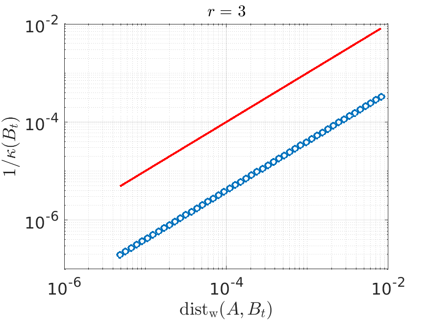
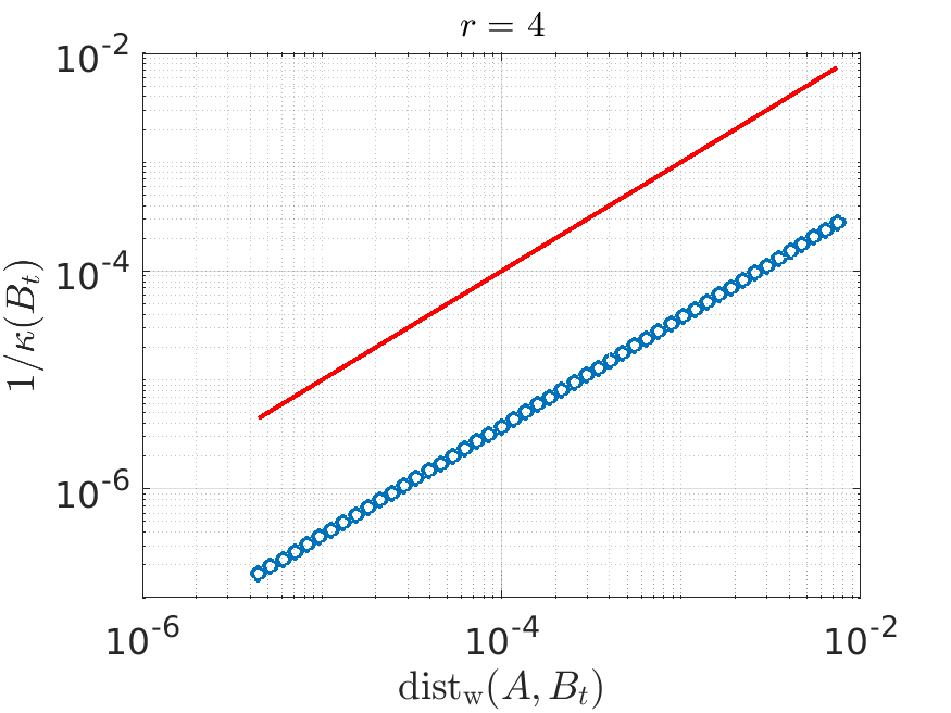
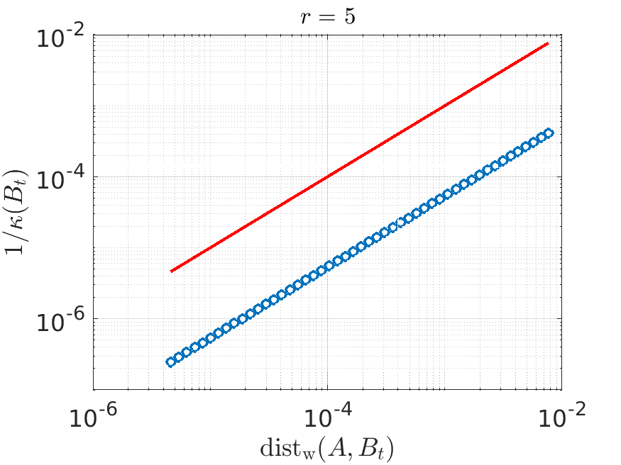
Figure 5.1. The blue data points compare the inverse condition number and the estimate of the weighted distance to the locus of ill-posed CPDs for the tensors described in Section 5. The red line illustrates where the data points would lie if the inequality in Theorem 1.3 were an equality. The gap between the red line and the blue data points is thus a measure for the sharpness of the bound in Theorem 1.3.

5.2. Distribution of the condition number

Figure 5.2. A log-log plot of the empirical complementary cumulative distribution function of the $(n-1)$th power of the condition number of random rank-$1$ tuples $(\mathfrak{A}_{1},\ldots,\mathfrak{A}_{7})$ in the space $\mathbb{R}^{7\times 7\times n}$ for $n=2,3,\ldots,7$, computed from $10^{7}$ samples. The dashed lines represent approximations of the form $a_{n}x^{-b_{n}}$ of the empirical ccdf for $i=2,3,\ldots,7$; the parameters $(a_{n},b_{n})$ for each case are given in Table 5.1.

We perform Monte Carlo experiments for providing additional numerical evidence for Theorems 1.4 and 1.1. To this end, we randomly sampled $10^{7}$ random rank-$1$ tuples $(\mathfrak{A}_{1},\ldots,\mathfrak{A}_{7})$ in $\mathbb{R}^{7\times 7\times n}$, where $n=2,3,\ldots,7$, and computed their condition numbers. We will abbreviate the random variable $\kappa(\mathfrak{A}_{1},\ldots,\mathfrak{A}_{7})$ to $\kappa$ from now onwards. These condition numbers are computed by constructing the $49n\times 7(12+n)$ block matrix $T=[U_{i}]_{i=1}^{7}$ from [8, Theorem 1.1], where the individual blocks $U_{i}$ are those from [8, equation (5.1)], and then computing the inverse of the least (i.e., the $7(12+n)$th) singular value of $T$. The outcome of this experiment is summarized in Figure 5.2, where we plot the complementary cumulative distribution function (ccdf) of the $(n-1)$th power of the condition number; recall that we know from Corollary 1.1 that $\mathbb{E}[\kappa^{n-1}]=\infty$.

It may appear at first glance that $\kappa^{n-1}$ behaves very erratically near the tails of the ccdfs in Figure 5.2. This phenomenon is entirely due to the sample error. Indeed, as we took $10^{7}$ samples, this means that in the empirical ccdf, there are $10^{k}$ data points between $10^{-7}\leq\mathrm{P}[\kappa^{n-1}>x]\leq 10^{-7+k}$. For $k=1$ or $2$, the resulting sample error is visually evident.

It is particularly noteworthy that all of the ccdfs in Figure 5.2 roughly appear to be shifted by a constant; the slope of the curves looks rather similar. In the figure, there are additional dashed lines that appear to capture the asymptotic behavior of the ccdfs of $\kappa^{n-1}$ quite well. These straight lines in the log-log plot correspond to a hypothesized model $a_{n}x^{-b_{n}}$ with $a_{n},b_{n}\geq 0$. In Table 5.1, we give the (rounded) parameter values for these dashed lines in Figure 5.2. By taking a log-transformation, fitting the model becomes a linear least squares problem, which was solved exactly. To avoid overfitting, we leave out the $9.9\cdot 10^{6}$ smallest condition numbers, that is, all data above the horizontal line $\mathrm{P}[\kappa^{n-1}>x]=10^{-2}$, as well as the $100$ largest condition numbers, i.e., the data below the horizontal line $\mathrm{P}[\kappa^{n-1}>x]=10^{-5}$. The motivation for this is as follows: the right tails of the ccdfs are corrupted by sampling errors, while for the left tails the model is clearly not valid. We are convinced that the hypothesized model is the correct one for very large condition numbers based on Theorem 1.3, which shows that a small distance from the ill-posed locus $\Sigma_{\mathbb{P}}$ the condition number grows at least like one over the distance, and the experiments from Section 5.1, which show that close to the ill-posed locus the growth of the condition number appears also to be bounded by a constant times the inverse distance to $\Sigma_{\mathbb{P}}$. In other words, close to $\Sigma_{\mathbb{P}}$, the condition number behaves, as determined experimentally, asymptotically as $\kappa(A)=\mathcal{O}\bigl{(}(\mathrm{dist}_{w}(A,\Sigma_{\mathbb{P}}))^{-1}\bigr{)}$.

$$\begin{array}[]{lrrrrrr}\hline\cr\hline\cr n&2&3&4&5&6&7\\ \hline\cr a_{n}&2328.45&447.54&656.27&1902.08&5210.73&13485.19\\ b_{n}&1.17713&1.00514&1.01091&1.01415&1.08573&1.20828\\ \hline\cr R^{2}&0.99994&0.99987&0.99975&0.99988&0.99940&0.99972\\ \hline\cr\hline\cr\end{array}$$

Table 5.1. Parameters $(n,a_{n},b_{n})$ of the model $a_{n}x^{-b_{n}}$ fitted to the empirical cumulative distribution function described in Figure 5.2. The row $R^{2}$ reports the coefficient of determination of the linear regression model $\log(a_{n})-b_{n}\log(x)$ on the log-transformed empirical data; $R^{2}=1$ means the model perfectly predicts the data.

From the above discussion, we can conclude that for sufficiently large $x$, say $x\geq\kappa_{0}$, the true cdf of $\kappa^{n-1}$, i.e., $F(x)=\mathrm{P}[\kappa^{n-1}\leq x]=1-\mathrm{P}[\kappa^{n-1}\geq x]$ is very well approximated by $1-a_{n}x^{-b_{n}}=\widetilde{F}(x).$ We can now employ the estimated cdfs to estimate the expected value of the $k$th power of the condition number $\kappa$ in the unknown cases $n=3,4,\ldots,7$ and $1\leq k\leq n-2$. We are unable to compute these cases analytically because, firstly, we do not know whether the codimension of $\overline{\Sigma_{\mathbb{P}}}$ is one, and, secondly, the techniques in this paper can prove only lower bounds on the condition number. We compute

$$\mathbb{E}[\kappa^{k}]=\mathbb{E}[(\kappa^{n-1})^{\frac{k}{n-1}}]=\int_{0}^{\infty}x^{\frac{k}{n-1}}\,\mathrm{d}F(x)=C+\int_{\kappa_{0}}^{\infty}x^{\frac{k}{n-1}}F^{\prime}(x)\mathrm{d}x\approx C^{\prime}+\int_{\kappa_{0}}^{\infty}x^{\frac{k}{n-1}}\widetilde{F}^{\prime}(x)\mathrm{d}x,$$

where in the last step we assume that the error term $E(x)=F^{\prime}(x)-\widetilde{F}^{\prime}(x)$ integrated against $x^{\frac{k}{n-1}}$ is at most a constant; this requires that the hypothesized model is asymptotically correct as $x\to\infty$, which seems reasonable based on the above experiments. So it follows that

$$\mathbb{E}[\kappa^{k}]\approx C^{\prime}+\int_{\kappa_{0}}^{\infty}a_{n}b_{n}x^{-b_{n}-1+\frac{k}{n-1}}\mathrm{d}x.$$

Note that the critical value for obtaining a finite integral is $k<(n-1)b_{n}$. Incidentally, the integral computed from the hypothesized model is finite for $n=2$, as $1<1.17713$, but we attribute this $17\%$ error of $b_{n}$ to the sample variance, as we have proved in Corollary 1.1 that the true integral is infinity. For $n\geq 3$, all of the hypothesized integrals with $1\leq k\leq n-2$ integrate to constants; the computed values $b_{n}$ would have to be off by $27\%$ before the case $n=5$ with $k=3$ integrates to infinity. This provides some indications that the expected value of the condition number $\kappa$ will be finite for $n_{1}\times n_{2}\times n_{3}$ tensors, provided that all $n_{i}\geq 3$. It is therefore unlikely that Corollary 1.1 may be improved by the techniques considered in this paper.

6. Conclusions

We presented a technique for establishing whether the average condition number of CPDs is infinite, namely Theorem 1.4. This is based on the partial condition number theorem, Theorem 1.3, that bounds the inverse condition number by a distance to the locus of ill-posed CPDs. Using this strategy, we showed that the average of powers of the condition numbers of random rank-$1$ tuples of length $r$ can be infinite in Corollary 1.1, depending on the codimension of the ill-posed locus. In particular, it was proved that the average condition number for $n_{1}\times n_{2}\times 2$ tensors is infinite. We are convinced that the inability to reduce the power in Corollary 1.1 to $1$ for $n_{1}\times n_{2}\times n_{3}$ tensors with $2\leq n_{1},n_{2},n_{3}\leq 10$, as shown in Proposition 3.7, along with the numerical experiments in Section 5.2, are a strong indication that the average condition number is finite for tensors for which $n_{1},n_{2},n_{3}\geq 3$.

The large gap in sensitivity between the case of $n_{1}\times n_{2}\times 2$ tensors and larger tensors has negative implications for the numerical stability of algorithms for computing CPDs based on a generalized eigendecomposition [[, such as those by]]LRA1993,Lorber1985,SK1990,SY1980, as is shown by [4].

The strategy presented in this article cannot prove that the average condition number is finite. However, we believe that the main components of our approach can be adapted to prove upper bounds on the average condition number, provided that one can establish a local converse to Theorem 1.3.

Appendix A Proof of Proposition 4.3

In this section we prove Proposition 4.3 to complete our study. We abbreviate $\mathbb{P}^{m-1}:=\mathbb{P}(\mathbb{R}^{m})$ in the following. Consider the following commutative diagram:

Herein, $\sigma$ as defined in 2.2 is an isometry by the definition, $\phi$ is defined as in the statement of the proposition, and $\iota$ is the Plücker embedding [25, Chapter 3.1.], which maps into the space of alternating tensors $\mathbb{P}(\wedge^{n}\mathbb{R}^{\Pi})$. Recall from [37, Section 2.6] that alternating tensors are linear combinations of alternating rank-1 tensors like

$$\mathbf{x}_{1}\wedge\cdots\wedge\mathbf{x}_{d}:=\frac{1}{d!}\sum_{\pi\in\mathfrak{S}_{d}}\operatorname{sgn}(\pi)\mathbf{x}_{\pi_{1}}\otimes\mathbf{x}_{\pi_{2}}\otimes\cdots\otimes\mathbf{x}_{\pi_{d}};$$

where $\mathfrak{S}_{d}$ is the permutation group on $\{1,\ldots,d\}$.

The image of the Plücker embedding $\mathscr{P}:=\iota(\mathrm{Gr}(\Pi,n))\subset\mathbb{P}\left(\wedge^{n}\mathbb{R}^{\Pi}\right)$ is a smooth variety called the Plücker variety. The Fubini–Study metric on $\mathbb{P}\left(\wedge^{n}\mathbb{R}^{\Pi}\right)$ makes $\mathscr{P}$ a Riemannian manifold. The Plücker embedding is an isometry; see, e.g., [28, Section 2] or [24, Chapter 3, Section 1.3].

Since $\sigma$ and $\iota$ are isometries, it follows from Lemma 4.2 that $\phi$ is an isometric immersion if and only if $\psi:=\iota\circ\phi\circ\sigma$ is an isometric immersion. We proceed by proving the latter. According to Definition 4.1, we have to prove that for all $p\in\mathbb{P}^{n_{1}-1}\times\cdots\times\mathbb{P}^{n_{d}-1}$ and for all $x,y\in\mathrm{T}_{p}{(\mathbb{P}^{n_{1}-1}\times\cdots\times\mathbb{P}^{n_{d}-1})}$ we have

$$\langle x,y\rangle_{\text{w}}=\langle(\mathrm{d}_{p}\psi)(x),(\mathrm{d}_{p}\psi)(y)\rangle.$$

However, the equality $2\langle x,y\rangle=\langle x-y,x-y\rangle-\langle x,x\rangle-\langle y,y\rangle$ shows that it suffices to prove

(A.1) $$\forall p\in\mathbb{P}^{n_{1}-1}\times\cdots\times\mathbb{P}^{n_{d}-1}:\forall x\in\mathrm{T}_{p}{(\mathbb{P}^{n_{1}-1}\times\cdots\times\mathbb{P}^{n_{d}-1})}:\langle x,x\rangle_{\text{w}}=\langle(\mathrm{d}_{p}\psi)(x),(\mathrm{d}_{p}\psi)(x)\rangle.$$

To show this, let $p\in\mathbb{P}^{n_{1}-1}\times\cdots\times\mathbb{P}^{n_{d}-1}$ and $x\in\mathrm{T}_{p}{(\mathbb{P}^{n_{1}-1}\times\cdots\times\mathbb{P}^{n_{d}-1})}$ be fixed and consider any smooth curve $\gamma:(-1,1)\to\mathbb{P}^{n_{1}-1}\times\cdots\times\mathbb{P}^{n_{d}-1}$ with $\gamma(0)=p$ and $\gamma^{\prime}(0)=x$. The action of the differential is computed as follows according to [38, Corollary 3.25]:

$$(\mathrm{d}_{p}\psi)(x)=\mathrm{d}_{0}(\psi\circ\gamma).$$

We compute the right-hand side of that equation. However, before taking derivatives, we first compute an expression for $(\psi\circ\gamma)(t)$.

Because $\mathrm{T}_{p}{(\mathbb{P}^{n_{1}-1}\times\cdots\times\mathbb{P}^{n_{d}-1})}=\mathrm{T}_{p_{1}}{\mathbb{P}^{n_{1}-1}}\times\cdots\times\mathrm{T}_{p_{d}}{\mathbb{P}^{n_{d}-1}},$ we can write $x=(x_{1},\ldots,x_{d})$ with $x_{i}\in\mathrm{T}_{p_{i}}{\mathbb{P}^{n_{i}-1}}$. For each $i$, we denote by $\mathbf{a}_{i}\in\mathbb{S}(\mathbb{R}^{n_{i}})$ a unit-norm representative for $p_{i}$, i.e., $p_{i}=[\mathbf{a}_{i}]$ with $\|\mathbf{a}_{i}\|\leavevmode\nobreak\ =\leavevmode\nobreak\ 1$ in the Euclidean norm. Letting $\mathbf{a}_{i}^{\perp}=\left\{\mathbf{u}\in\mathbb{R}^{n_{i}}\mid\langle\mathbf{u},\mathbf{a}_{i}\rangle=0\right\}$ denote the orthogonal complement of $\mathbf{a}_{i}$ in $\mathbb{R}^{n_{i}}$, we can then identify $\mathbf{a}_{i}^{\perp}=\mathrm{T}_{p_{i}}{\mathbb{P}^{n_{i}-1}}$ by 2.3. Moreover, because $\mathbf{a}_{i}$ is of unit norm, the Fubini–Study metric on $\mathrm{T}_{p_{i}}{\mathbb{P}^{n_{i}-1}}$ is given by the Euclidean inner product on the linear subspace $\mathbf{a}_{i}^{\perp}$. Now, let $\mathbf{x}_{i}$ denote the unique vector in $\mathbf{a}_{i}^{\perp}$ corresponding to $x_{i}$. The sphere $\mathbb{S}(\mathbb{R}^{n_{i}})$ is a smooth manifold, so we find a curve $\gamma_{i}:(-1,1)\to\mathbb{S}(\mathbb{R}^{n_{i}})$ with $\gamma_{i}(0)=\mathbf{a}_{i}$ and $\gamma_{i}^{\prime}(0)=\mathbf{x}_{i}$. Without loss of generality we assume that $\gamma_{i}$ is the exponential map [38, Chapter 20]. We claim that we can write $\gamma$ as $\gamma(t)=(\pi_{1}\circ\gamma_{1}(t),\ldots,\pi_{d}\circ\gamma_{d}(t))$, where $\pi_{i}:\mathbb{S}(\mathbb{R}^{n_{i}})\to\mathbb{P}^{n_{i}-1}$ is the canonical projection. Indeed, we have $\gamma(0)=([\mathbf{a}_{1}],\ldots,[\mathbf{a}_{d}])=p$ and

$$\gamma^{\prime}(0)=\bigl{(}(\pi_{1}\circ\gamma_{1})^{\prime}(0),\ldots,(\pi_{d}\circ\gamma_{d})^{\prime}(0)\bigr{)} =\bigl{(}\mathrm{P}_{(\mathbf{a}_{1}^{\perp})}\gamma_{1}^{\prime}(0),\ldots,\mathrm{P}_{(\mathbf{a}_{d}^{\perp})}\gamma_{d}^{\prime}(0)\bigr{)}$$

$$=\bigl{(}\mathrm{P}_{(\mathbf{a}_{1}^{\perp})}\mathbf{x}_{1},\ldots,\mathrm{P}_{(\mathbf{a}_{d}^{\perp})}\mathbf{x}_{d}\bigr{)}=\bigl{(}\mathbf{x}_{1},\ldots,\mathbf{x}_{d}\bigr{)}=x,$$

where $\mathrm{P}_{A}$ denotes the orthogonal projection onto the linear space $A$, where the second equality is due to [12, Lemma 14.8], and where the last step is due to the identification $\mathbf{a}_{i}^{\perp}\simeq\mathrm{T}_{p_{i}}{\mathbb{P}^{n_{i}-1}}$. This shows $(\psi\circ\gamma)(t)=\psi(\pi_{1}\circ\gamma_{1}(t),\ldots,\pi_{d}\circ\gamma_{d}(t))$. Recall that $\psi=\iota\circ\phi\circ\sigma$ and that

$$(\phi\circ\sigma\circ\gamma)(t)=\mathrm{T}_{\gamma_{1}(t)\otimes\cdots\otimes\gamma_{d}(t)}{\,}\mathcal{S}.$$

Hence, $(\psi\circ\gamma)(t)=\psi(\mathrm{T}_{\gamma_{1}(t)\otimes\cdots\otimes\gamma_{d}(t)}{\,}\mathcal{S})$. To compute the latter we must give a basis for the tangent space $\mathrm{T}_{\gamma_{1}(t)\otimes\cdots\otimes\gamma_{d}(t)}{\,}\mathcal{S}$. To do so, let us denote by $\{\mathbf{u}_{1}^{i}(t),\mathbf{u}_{2}^{i}(t),\ldots,\mathbf{u}_{n_{i}-1}^{i}(t)\}$ an orthonormal basis for the orthogonal complement of $\gamma_{i}(t)$; such a moving orthonormal basis is called an orthonormal frame. Then, by [37, Section 4.6.2] a basis for $\mathrm{T}_{\gamma_{1}(t)\otimes\cdots\otimes\gamma_{d}(t)}{\mathcal{S}}$ is given by

$$\mathcal{B}(t)=\left\{\mathfrak{A}(t)\right\}\cup\left\{\mathfrak{A}_{(i,j)}(t)\mid 1\leq i\leq d,1\leq j\leq n_{i}-1\right\},$$

where

(A.2) $$\mathfrak{A}(t):= \gamma_{1}(t)\otimes\cdots\otimes\gamma_{d}(t)\;\text{ and }\;$$

$$\mathfrak{A}_{(i,j)}(t)= \gamma_{1}(t)\otimes\cdots\otimes\gamma_{i-1}(t)\otimes\mathbf{u}_{j}^{i}(t)\otimes\gamma_{i+1}(t)\otimes\cdots\otimes\gamma_{d}(t).$$

If we let $\pi$ denote the canonical projection $\pi:\wedge^{n}\mathbb{R}^{\Pi}\to\mathbb{P}\left(\wedge^{n}\mathbb{R}^{\Pi}\right)$, then we find

(A.3) $$(\psi\circ\gamma)(t)=\iota(\mathrm{span}\,\mathcal{B}(t))=\pi\left(\mathfrak{A}(t)\wedge\Biggl{(}\bigwedge_{i=1}^{d}\bigwedge_{j=1}^{n_{i}-1}\mathfrak{A}_{(i,j)}(t)\Biggr{)}\right);$$

see [25, Chapter 3.1.C]. Note in particular that the right-hand side of A.3 is independent of the specific choice of the orthonormal bases $\mathcal{B}(t)$, because the exterior product of another basis is just a scalar multiple of the basis we chose (below we make a specific choice of $\mathcal{B}(t)$ that simplifies subsequent computations). In the following let

$$\mathbf{g}(t):=\mathfrak{A}(t)\wedge\Biggl{(}\bigwedge_{i=1}^{d}\bigwedge_{j=1}^{n_{i}-1}\mathfrak{A}_{(i,j)}(t)\Biggr{)}.$$

We are now prepared to compute the derivative of $(\psi\circ\gamma)(t)=(\pi\circ\mathbf{g})(t)=[\mathbf{g}(t)]$. According to [12, Lemma 14.8], we have

$$\mathrm{d}_{0}(\psi\circ\gamma)=\mathrm{P}_{(\mathbf{g}(0))^{\perp}}\frac{\mathbf{g}^{\prime}(0)}{\|\mathbf{g}(0)\|}.$$

We will first prove that $\|\mathbf{g}(t)\|=1$, which entails that $\mathbf{g}(t)\subset\mathbb{S}(\wedge^{n}\mathbb{R}^{\Pi})$ so that

$$\mathrm{d}_{0}(\psi\circ\gamma)=\mathrm{P}_{(\mathbf{g}(0))^{\perp}}\mathbf{g}^{\prime}(0)=\mathbf{g}^{\prime}(0)=\mathrm{d}_{0}\mathbf{g},$$

as $\mathbf{g}^{\prime}(t)$ would in this case be contained in the tangent space to the sphere over $\wedge^{n}\mathbb{R}^{\Pi}$. We now need the following standard result.

Lemma A.1.

We have the following:

1. For $1\leq k\leq d$, let $\mathbf{x}_{k},\mathbf{y}_{k}\in\mathbb{R}^{n_{k}}$, and let $\langle\cdot,\cdot\rangle$ denote the standard Euclidean inner product. Then, the inner product of rank-1 tensors satisfies $\langle\mathbf{x}_{1}\otimes\cdots\otimes\mathbf{x}_{d},\,\mathbf{y}_{1}\otimes\cdots\otimes\mathbf{y}_{d}\rangle=\prod_{j=1}^{d}\langle\mathbf{x}_{j},\mathbf{y}_{j}\rangle$.

2. Let $\mathbf{x}_{1},\ldots,\mathbf{x}_{d},\mathbf{y}_{1},\ldots,\mathbf{y}_{d}\in\mathbb{R}^{m}$. Let $\langle\cdot,\cdot\rangle$ be the standard Euclidean inner product. Then, the inner product of skew-symmetric rank-1 tensors satisfies $\langle\mathbf{x}_{1}\wedge\cdots\wedge\mathbf{x}_{d},\,\mathbf{y}_{1}\wedge\cdots\wedge\mathbf{y}_{d}\rangle=\det\bigl{(}[\langle\mathbf{x}_{i},\mathbf{y}_{j}\rangle]_{i,j=1}^{d}\bigr{)}.$

3. Whenever $\{\mathbf{x}_{1},\ldots,\mathbf{x}_{d}\}$ is a linearly dependent set, we have $\mathbf{x}_{1}\wedge\cdots\wedge\mathbf{x}_{d}=0.$

Proof.

For the first point see, e.g., [29, Section 4.5]. For the second see, e.g., [27, Section 4.8] or [38, Proposition 14.11]. The third is a consequence of the second point. ∎

Using the computation rules for inner products from Lemma A.1 we find

(A.4) $$\langle\mathfrak{A}(t),\mathfrak{A}(t)\rangle =\prod_{i=1}^{d}\langle\gamma_{i}(t),\gamma_{i}(t)\rangle=1;$$

(A.5) $$\langle\mathfrak{A}(t),\mathfrak{A}_{(i,j)}(t)\rangle =\langle\gamma_{i}(t),\mathbf{u}_{j}^{i}(t)\rangle\prod_{k\neq i}\langle\gamma_{k}(t),\gamma_{k}(t)\rangle=0;$$

(A.6) $$\langle\mathfrak{A}_{(i,j)}(t),\mathfrak{A}_{(k,\ell)}(t)\rangle =\begin{cases}1,&\text{if }(i,j)=(k,\ell),\\ 0,&\text{else.}\end{cases}$$

In other words, $\mathcal{B}(t)$ is an orthonormal basis for $\mathrm{T}_{\mathfrak{A}(t)}{\mathcal{S}}=\mathrm{T}_{\gamma_{1}(t)\otimes\cdots\otimes\gamma_{d}(t)}{\mathcal{S}}$. By Lemma A.1, we have

$$\langle\mathbf{g}(t),\mathbf{g}(t)\rangle=\det\begin{bmatrix}\langle\mathfrak{A}(t),\mathfrak{A}(t)\rangle&\langle\mathfrak{A}(t),\mathfrak{A}_{(1,1)}(t)\rangle&\cdots&\langle\mathfrak{A}(t),\mathfrak{A}_{(d,n_{d})}(t)\rangle\\ \langle\mathfrak{A}_{(1,1)}(t),\mathfrak{A}(t)\rangle&\langle\mathfrak{A}_{(1,1)}(t),\mathfrak{A}_{(1,1)}(t)\rangle&\cdots&\langle\mathfrak{A}_{(1,1)}(t),\mathfrak{A}_{(d,n_{d})}(t)\rangle\\ \vdots&\vdots&\ddots&\vdots\\ \langle\mathfrak{A}_{(d,n_{d})}(t),\mathfrak{A}(t)\rangle&\langle\mathfrak{A}_{(d,n_{d})}(t),\mathfrak{A}_{(1,1)}(t)\rangle&\cdots&\langle\mathfrak{A}_{(d,n_{d})}(t),\mathfrak{A}_{(d,n_{d})}(t)\rangle\end{bmatrix},$$

which equals $\det I_{n}=1$.

It now only remains to compute $\mathrm{d}_{0}\mathbf{g}$. For this we have the following result.

Lemma A.2.

Let $\mathfrak{A}:=\mathfrak{A}(0)$ and $\mathfrak{A}_{(i,j)}:=\mathfrak{A}_{(i,j)}(0)$ and write

$$\mathbf{f}_{(i,j)}:=\mathfrak{A}\wedge\mathfrak{A}_{(1,1)}\wedge\cdots\wedge\mathfrak{A}_{(i,j-1)}\wedge\mathfrak{A}_{(i,j)}^{\prime}(0)\wedge\mathfrak{A}_{(i,j+1)}\wedge\cdots\wedge\mathfrak{A}_{(p,n_{d}-1)}.$$

The differential satisfies $\mathrm{d}_{0}\mathbf{g}=\sum_{i=1}^{d}\sum_{j=1}^{n_{i}-1}\mathbf{f}_{(i,j)},$ where $\left\langle\mathbf{f}_{(i,j)},\mathbf{f}_{(k,\ell)}\right\rangle=\delta_{ik}\delta_{j\ell}\sum_{1\leq\lambda\neq i\leq d}\langle\mathbf{x}_{\lambda},\mathbf{x}_{\lambda}\rangle,$ where $\delta_{ij}$ is the Kronecker delta.

We prove this lemma at the end of this section. We can now prove A.1. From Lemma A.2, we find

$$\langle(\mathrm{d}_{p}\psi)(x),(\mathrm{d}_{p}\psi)(x)\rangle=\langle\mathrm{d}_{0}\mathbf{g},\mathrm{d}_{0}\mathbf{g}\rangle=\left\langle\sum_{i=1}^{d}\sum_{j=1}^{n_{i}-1}\mathbf{f}_{(i,j)},\sum_{k=1}^{d}\sum_{\ell=1}^{n_{k}-1}\mathbf{f}_{(k,\ell)}\right\rangle=\sum_{i=1}^{d}\sum_{j=1}^{n_{i}-1}\sum_{1\leq\lambda\neq i\leq d}\langle\mathbf{x}_{\lambda},\mathbf{x}_{\lambda}\rangle.$$

Reordering the terms, one finds

$$\langle(\mathrm{d}_{p}\psi)(x),(\mathrm{d}_{p}\psi)(x)\rangle=\sum_{i=1}^{d}\langle\mathbf{x}_{i},\mathbf{x}_{i}\rangle\sum_{1\leq\lambda\neq i\leq d}\sum_{j=1}^{n_{\lambda}-1}1=\sum_{i=1}^{d}\langle\mathbf{x}_{i},\mathbf{x}_{i}\rangle\cdot(n-n_{i})=\langle\mathbf{x},\mathbf{x}\rangle_{\mathrm{w}},$$

where the penultimate equality follows from the formula $n=1+\sum_{i=1}^{d}(n_{i}-1)$ in 2.1. This proves A.1 so that $\phi$ is an isometric map.

Finally, A.1 also entails that $\phi$ is an immersion. Indeed, for an immersion it is required that $\mathrm{d}_{p}\psi$ is injective. Suppose that this is false, then there is a nonzero $x\in\mathrm{T}_{p}{(\mathbb{P}^{n_{1}-1}\times\cdots\times\mathbb{P}^{n_{d}-1})}$ with corresponding nonzero $\mathbf{x}$ such that

$$0=\langle 0,0\rangle=\langle(\mathrm{d}_{p}\psi)(x),(\mathrm{d}_{p}\psi)(x)\rangle=\langle\mathbf{x},\mathbf{x}\rangle_{\mathrm{w}}>0,$$

which is a contraction. Consequently, $\phi$ is an isometric immersion, concluding the proof.∎

It remains to prove Lemma A.2.

Proof of Lemma A.2.

Recall that we have put $\mathbf{a}_{i}:=\gamma_{i}(0)\in\mathbb{S}(\mathbb{R}^{n_{i}})$ and $\mathbf{x}_{i}:=\gamma_{i}^{\prime}(0)\in\mathrm{T}_{\mathbf{a}_{i}}{\mathbb{S}(\mathbb{R}^{n_{i}})}$ for $1\leq i\leq d$. Without restriction we can assume that $\gamma_{i}$ is contained in the great circle through $\mathbf{a}_{i}$ and $\mathbf{x}_{i}$. As argued above, we have the freedom of choice of an orthonormal basis of each $\gamma_{i}(t)^{\perp}$. To simplify computations we make the following choice.

For all $i$, let $\mathbf{u}_{2}^{i},\ldots,\mathbf{u}_{n_{i}-1}^{i}$ be an orthonormal basis for $\mathbf{a}_{i}^{\perp}\cap\,\mathbf{x}_{i}^{\perp}$ and consider the orthogonal transformation $U$ that rotates $\mathbf{a}_{i}$ to $\|\mathbf{x}_{i}\|^{-1}\mathbf{x}_{i}$, $\mathbf{x}_{i}$ to $-\|\mathbf{x}_{i}\|\mathbf{a}_{i}$ and leaves $\left\{\mathbf{u}_{2}^{i},\ldots,\mathbf{u}_{n-1}^{i}\right\}$ fixed. Then, we define the following curves (which expect for the first one are all constant).

$$\mathbf{u}_{1}^{i}(t):=U\gamma_{i}(t),\quad\mathbf{u}_{2}^{i}(t):=\mathbf{u}_{2}^{i},\quad\ldots\quad\mathbf{u}_{n_{i}-1}^{i}(t):=\mathbf{u}_{n_{i}-1}^{i}.$$

By construction $\{\mathbf{u}_{1}^{i}(t),\mathbf{u}_{2}^{i}(t),\ldots,\mathbf{u}_{n-1}^{i}(t)\}$ is an orthonormal basis for the orthogonal complement of $\gamma_{i}(t)$ for all $t$. We have

(A.7) $$\mathrm{d}_{0}\mathbf{u}_{1}^{i}(t)=U\gamma_{i}^{\prime}(0)=-\|\mathbf{x}_{i}\|\mathbf{a}_{i},\quad\mathrm{d}_{0}\mathbf{u}_{2}^{i}(t)=\cdots=\mathrm{d}_{0}\mathbf{u}_{n_{i}-1}^{i}(t)=0.$$

Figure A.1. A sketch of the orthonormal frame $\{\gamma_{i}(t),U\gamma_{i}(t),\mathbf{u}_{2}^{i}(t),\ldots,\mathbf{u}_{n_{i}-1}^{i}(t)\}$.

We will use this choice of orthonormal bases for the remainder of the proof. By the definition of $\mathbf{g}(t)$ and the product rule of differentiation, the first term of $\mathrm{d}_{0}\mathbf{g}$ is $\mathfrak{A}^{\prime}(0)\wedge\bigwedge_{i=1}^{d}\bigwedge_{j=1}^{n_{i}-1}\mathfrak{A}_{(i,j)}$. We have

(A.8) $$\mathfrak{A}^{\prime}(0)=\sum_{\lambda=1}^{d}\mathbf{a}_{1}\otimes\cdots\otimes\mathbf{a}_{\lambda-1}\otimes\mathbf{x}_{\lambda}\otimes\mathbf{a}_{\lambda+1}\otimes\cdots\otimes\mathbf{a}_{d}=\sum_{\lambda=1}^{d}\lVert\mathbf{x}_{\lambda}\rVert\mathfrak{A}_{(\lambda,1)}.$$

Hence, from the multilinearity of the exterior product it follows that the first term of $\mathrm{d}_{0}\mathbf{g}$ is

$$\sum_{\lambda=1}^{d}\lVert\mathbf{x}^{\lambda}\rVert\left(\mathfrak{A}_{(\lambda,1)}\wedge\mathfrak{A}_{(1,1)}\wedge\cdots\wedge\mathfrak{A}_{(d,n_{d}-1)}\right)=\sum_{\lambda}0=0.$$

This implies that all of the terms of $\mathrm{d}_{0}\mathbf{g}$ involve $\mathfrak{A}_{(i,j)}^{\prime}(0)$ for some $(i,j)$. From A.2, we find

$$\mathfrak{A}_{(i,j)}^{\prime}(0)=\sum_{\lambda=1}^{d}\mathfrak{A}_{(i,j)}^{\lambda},$$

where, using the shorthand notation $\mathbf{u}_{j}^{i}=\mathbf{u}_{j}^{i}(0)$, we have put

$$\mathfrak{A}_{(i,j)}^{\lambda}:=\begin{cases}\mathbf{a}_{1}\otimes\cdots\otimes\mathbf{a}_{\lambda-1}\otimes\mathbf{x}_{\lambda}\otimes\mathbf{a}_{\lambda+1}\otimes\cdots\otimes\mathbf{a}_{i-1}\otimes\mathbf{u}_{j}^{i}\otimes\mathbf{a}_{i+1}\otimes\cdots\otimes\mathbf{a}_{d}&\text{if }\lambda\neq i,\\ \mathbf{a}^{1}\otimes\cdots\otimes\mathbf{a}^{i-1}\otimes\mathrm{d}_{0}\mathbf{u}_{j}^{i}(t)\otimes\mathbf{a}^{i+1}\otimes\cdots\otimes\mathbf{a}^{d},&\text{otherwise}.\end{cases}$$

Recall from A.7 that $\mathrm{d}_{0}\mathbf{u}_{1}^{i}(t)=-\|\mathbf{x}_{i}\|\mathbf{a}_{i}$, while for $j>1$ we have $\mathrm{d}_{0}\mathbf{u}_{j}^{i}(t)=0$. Hence,

$$\mathfrak{A}_{(i,j)}^{\lambda}:=\begin{cases}\mathbf{a}_{1}\otimes\cdots\otimes\mathbf{a}_{\lambda-1}\otimes\mathbf{x}_{\lambda}\otimes\mathbf{a}_{\lambda+1}\otimes\cdots\otimes\mathbf{a}_{i-1}\otimes\mathbf{u}_{j}^{i}\otimes\mathbf{a}_{i+1}\otimes\cdots\otimes\mathbf{a}_{d}&\text{if }\lambda\neq i,\\ \mathbf{a}^{1}\otimes\cdots\otimes\mathbf{a}^{i-1}\otimes(-\|\mathbf{x}_{i}\|\mathbf{a}_{i})\otimes\mathbf{a}^{i+1}\otimes\cdots\otimes\mathbf{a}^{d},&\text{if }(\lambda,j)=(i,1),\\ 0&\text{otherwise}.\end{cases}$$

Then,

(A.9) $$\mathbf{f}_{(i,j)} =s_{(i,j)}\,\mathfrak{A}\wedge\left(\sum_{\lambda=1}^{d}\mathfrak{A}_{(i,j)}^{\lambda}\right)\wedge\bigwedge_{i=1}^{d}\bigwedge_{1\leq j\neq i<n_{i}}\mathfrak{A}_{(i,j)}$$

$$=s_{(i,j)}\sum_{1\leq\lambda\neq i\leq d}\mathfrak{A}\wedge\mathfrak{A}_{(i,j)}^{\lambda}\wedge\bigwedge_{i=1}^{d}\bigwedge_{1\leq j\neq i<n_{i}}\mathfrak{A}_{(i,j)}=:s_{(i,j)}\sum_{1\leq\lambda\neq i\leq d}\mathbf{f}_{(i,j)}^{\lambda},$$

where $s_{(i,j)}\in\{-1,1\}$ is the sign of the permutation for moving $\mathfrak{A}_{(i,j)}^{\prime}(0)$ to the second position in the exterior product. We continue by computing for $\lambda\neq i$ and $\mu\neq k$ the value

$$\langle\mathbf{f}_{(i,j)}^{\lambda},\mathbf{f}_{(k,\ell)}^{\mu}\rangle=\det\bigl{(}B_{(i,j),\lambda}^{T}B_{(k,\ell),\mu}\bigr{)},\text{ where }\;B_{(i,j),\lambda}:=\begin{bmatrix}\mathfrak{A}&\mathfrak{A}_{(i,j)}^{\lambda}&[[\mathfrak{A}_{(i,j)}]_{j\neq i}]_{i=1}^{d}\end{bmatrix};$$

herein, the column vectors should be interpreted as vectorized tensors. Recall that $\langle\mathbf{a}_{i},\mathbf{x}_{i}\rangle=0$ and that $\langle\mathbf{a}_{i},\mathbf{u}_{j}^{i}\rangle=0$ for all $i,j$. Then, it follows from Lemma A.1 and direct computations that for $\lambda\neq i$ and $\mu\neq k$, we have

$$\langle\mathfrak{A},\mathfrak{A}_{(k,\ell)}^{\mu}\rangle =\langle\mathfrak{A},\mathfrak{A}_{(k,\ell)}\rangle=0,\quad\langle\mathfrak{A}_{(i,j)}^{\lambda},\mathfrak{A}_{(k,\ell)}^{\mu}\rangle=\delta_{ik}\delta_{j\ell}\delta_{\lambda\mu}\|\mathbf{x}_{\lambda}\|^{2},\quad\text{and}\quad\langle\mathfrak{A}_{(i,j)}^{\lambda},\mathfrak{A}_{(k,\ell)}\rangle=0.$$

We distinguish between two cases. If $(i,j)\neq(k,\ell)$, $\lambda\neq i$ and $\mu\neq k$, it follows from the above equations that the row of $(B_{(i,j),\lambda})^{T}B_{(k,\ell),\mu}$ consisting of

$$\begin{bmatrix}\langle\mathfrak{A}_{(i,j)}^{\lambda},\mathfrak{A}\rangle&\langle\mathfrak{A}_{(i,j)}^{\lambda},\mathfrak{A}_{(k,\ell)}^{\mu}\rangle&[[\langle\mathfrak{A}_{(i,j)}^{\lambda},\mathfrak{A}_{(k,\ell)}\rangle]_{\ell\neq k}]_{k}\end{bmatrix}$$

is a zero row, which implies that $\left\langle\mathbf{f}_{(i,j),\lambda},\mathbf{f}_{(k,\ell),\mu}\right\rangle=0$. On the other hand, if $(i,j)=(k,\ell)$, $\lambda\neq i$ and $\mu\neq k$, then it follows from the above equations that $B_{(i,j),\lambda}^{T}B_{(i,j),\mu}$ is a diagonal matrix, namely

$$B_{(i,j),\lambda}^{T}B_{(i,j),\mu}=\operatorname{diag}(1,\langle\mathfrak{A}_{(i,j)}^{\lambda},\mathfrak{A}_{(i,j)}^{\mu}\rangle,1,\ldots,1).$$

Its determinant is then $\langle\mathfrak{A}_{(i,j)}^{\lambda},\mathfrak{A}_{(i,j)}^{\mu}\rangle=\delta_{\lambda\mu}\|\mathbf{x}_{\lambda}\|^{2}$. Therefore,

(A.10) $$\langle\mathbf{f}_{(i,j)}^{\lambda},\mathbf{f}_{(k,\ell)}^{\mu}\rangle=\delta_{ik}\delta_{j\ell}\delta_{\lambda\mu}\|\mathbf{x}_{\lambda}\|^{2}.$$

Finally, we can compute $\langle\mathbf{f}_{(i,j)},\mathbf{f}_{(k,\ell)}\rangle$. From A.9,

$$\langle\mathbf{f}_{(i,j)},\mathbf{f}_{(k,\ell)}\rangle=s_{(i,j)}s_{(k,\ell)}\left\langle\sum_{1\leq\lambda\neq i\leq d}\mathbf{f}_{(i,j)}^{\lambda},\sum_{1\leq\mu\neq k\leq d}\mathbf{f}_{(k,\ell)}^{\mu}\right\rangle=s_{(i,j)}s_{(k,\ell)}\sum_{1\leq\lambda\neq i\leq d}\delta_{ik}\delta_{j\ell}\|\mathbf{x}_{\lambda}\|^{2},$$

which is zero unless $(i,j)=(k,\ell)$. For $(i,j)=(k,\ell)$, we find

$$\|\mathbf{f}_{(i,j)}\|^{2}=s_{(i,j)}^{2}\sum_{1\leq\lambda\neq i\leq d}\|\mathbf{x}_{\lambda}\|^{2}=\sum_{1\leq\lambda\neq i\leq d}\|\mathbf{x}_{\lambda}\|^{2},$$

proving the result. ∎

References

• [1] H. Abo, G. Ottaviani, and C. Peterson, Induction for secant varieties of Segre varieties, Trans. Amer. Math. Soc. 361 (2009), 767–792.
• [2] E. S. Allman, C. Matias, and J. A. Rhodes, Identifiability of parameters in latent structure models with many observed variables, Ann. Statist. 37 (2009), no. 6A, 3099–3132.
• [3] A. Anandkumar, R. Ge, D. Hsu, S. M. Kakade, and M. Telgarsky, Tensor decompositions for learning latent variable models, J. Mach. Learn. Res. 15 (2014), 2773–2832.
• [4] C. Beltrán, P. Breiding, and N. Vannieuwenhoven, Computing the tensor rank decomposition via a generalized eigendecomposition is not stable, arXiv (2018).
• [5] Å. Björck and Gene H. Golub, Numerical methods for computing angles between linear subspaces, Math. Comp. 27 (1973), no. 123, 579–594.
• [6] C. Bocci, L. Chiantini, and G. Ottaviani, Refined methods for the identifiability of tensors, Ann. Mat. Pura Appl. 193 (2014), 1691–1702.
• [7] P. Breiding, Numerical and statistical aspects of tensor decompositions, PhD Thesis, Technische Universität Berlin, 2017, http://dx.doi.org/10.14279/depositonce-6148.
• [8] P. Breiding and N. Vannieuwenhoven, The condition number of join decompositions, SIAM J. Matrix Anal. Appl. 39 (2018), no. 1, 287–309.
• [9] by same author, Convergence analysis of Riemannian Gauss-Newton methods and its connection with the geometric condition number, Appl. Math. Letters 78 (2018), 42–50.
• [10] by same author, A Riemannian trust region method for the canonical tensor rank approximation problem, arXiv:1709.00033 (2018).
• [11] P. Bürgisser, M. Clausen, and M. A. Shokrollahi, Algebraic Complexity Theory, Grundlehren der mathematischen Wissenshaften, vol. 315, Springer, Berlin, Germany, 1997.
• [12] P. Bürgisser and F. Cucker, Condition: The Geometry of Numerical Algorithms, Grundlehren der mathematischen Wissenschaften, vol. 349, Springer, Heidelberg, 2013. MR 3098452
• [13] L. Chiantini and G. Ottaviani, On generic identifiability of $3$-tensors of small rank, SIAM J. Matrix Anal. Appl. 33 (2012), no. 3, 1018–1037.
• [14] L. Chiantini, G. Ottaviani, and N. Vannieuwenhoven, An algorithm for generic and low-rank specific identifiability of complex tensors, SIAM J. Matrix Anal. Appl. 35 (2014), no. 4, 1265–1287.
• [15] P. Comon, Independent component analysis, a new concept?, Signal Proc. 36 (1994), no. 3, 287–314.
• [16] P. Comon and C. Jutten, Handbook of Blind Source Separation: Independent Component Analysis and Applications, Elsevier, 2010.
• [17] D. Cox, J. Little, and D. O’Shea, Ideals, varieties, and algorithms, 4 ed., Undergraduate Texts in Mathematics, Springer, 2015.
• [18] F. Cucker, Probabilistic analyses of condition numbers, Acta Numerica (2016), 321–382.
• [19] V. de Silva and L.-H. Lim, Tensor rank and the ill-posedness of the best low-rank approximation problem, SIAM J. Matrix Anal. Appl. 30 (2008), no. 3, 1084–1127.
• [20] J. W. Demmel, The geometry of ill-conditioning, J. Complexity 3 (1987), no. 2, 201–229.
• [21] by same author, On condition numbers and the distance to the nearest ill-posed problem, Numer. Math. 51 (1987), no. 3, 251–289.
• [22] M. do Carmo, Riemannian Geometry, Birhäuser, 1993.
• [23] C. Eckart and G. Young, A principal axis transformation for non-Hermitian matrices, Bull. Am. Math. Soc. 45 (1939), 118–121.
• [24] D. B. Fuchs, Topology II, Encyclopaedia of Mathematical Sciences, vol. 24, ch. Classical Manifolds, pp. 199–251, Springer–Verlag, Berlin, Heidelberg, 2004.
• [25] I.M. Gelfand, M. M. Kapranov, and A. V. Zelevinsky, Discriminants, Resultants and Multidimensional Determinants, Modern Birkhäuser Classics, Birkhäuser, 1994.
• [26] D. Grayson and M. Stillman, Macaulay 2, a software system for research in algebraic geometry, \urlwww.math.uiuc.edu/Macaulay2, 2018, Last accessed June 2, 2018.
• [27] W. H. Greub, Multilinear algebra, Springer-Verlag, 1978.
• [28] P. Griffiths, On Cartan’s method of Lie groups and moving frames as applied to uniqueness and existence questions in differential geometry, Duke Math. J. 41 (1974), no. 4, 775–814.
• [29] W. Hackbusch, Tensor Spaces and Numerical Tensor Calculus, Springer Series in Computational Mathematics, vol. 42, Springer-Verlag, 2012.
• [30] J. Harris, Algebraic Geometry, A First Course, Graduate Text in Mathematics, vol. 133, Springer-Verlag, 1992.
• [31] N. J. Higham, Accuracy and stability of numerical algorithms, 2 ed., Society for Industrial and Applied Mathematics, 1996.
• [32] F. L. Hitchcock, The expression of a tensor or a polyadic as a sum of products, J. Math. Phys. 6 (1927), 164–189.
• [33] D. Hough, Explaining and ameliorating the condition of zeros of polynomials, PhD Thesis, Mathematics Department, University of California, Berkeley, 1977.
• [34] J. Håstad, Tensor rank is NP-complete, J. Algorithms 11 (1990), no. 4, 644–654.
• [35] W. Kahan, Numerical linear algebra, Can. Math. Bull. 9 (1966), 757–801.
• [36] P. M. Kroonenberg, Applied Multiway Data Analysis, Wiley series in probability and statistics, John Wiley & Sons, Hoboken, New Jersey, 2008.
• [37] J. M. Landsberg, Tensors: Geometry and Applications, Graduate Studies in Mathematics, vol. 128, AMS, Providence, Rhode Island, 2012.
• [38] J. M. Lee, Introduction to Smooth Manifolds, second ed., Graduate Texts in Mathematics, vol. 218, Springer, New York, USA, 2013.
• [39] Kurt Leichtweiss, Zur riemannschen geometrie in grassmannschen mannigfaltigkeiten, Math. Z. 76 (1961), 334–366.
• [40] MATLAB, R2017b, Natick, Massachusetts, 2017.
• [41] P. McCullagh, Tensor Methods in Statistics, Monographs on statistics and applied probability, Chapman and Hall, New York, 1987.
• [42] N. D. Sidiropoulos, L. De Lathauwer, X. Fu, K. Huang, E. E. Papalexakis, and Ch. Faloutsos, Tensor decomposition for signal processing and machine learning, IEEE Trans. Signal Process. 65 (2017), no. 13, 3551–3582.
• [43] A. Smilde, R. Bro, and P. Geladi, Multi-way Analysis: Applications in the Chemical Sciences, John Wiley & Sons, Hoboken, New Jersey, 2004.
• [44] M. Spivak, Calculus on manifolds: A modern approach to classical theorems of advanced calcalus, Addison-Wesley, 1965.
• [45] N. Vannieuwenhoven, A condition number for the tensor rank decomposition, Linear Algebra Appl. 535 (2017), 35–86.
• [46] J. H. Wilkinson, Note on matrices with a very ill-conditioned eigenproblem, Numer. Math. 19 (1972), 176–178.
• [47] K. Ye and L.-H. Lim, Schubert varieties and distances between subspaces of different dimensions, SIAM J. Matrix Anal. Appl. 37 (2016), no. 3, 1176–1197.