Abstract

Computing the partition function $Z$ of a discrete graphical model is a fundamental inference challenge. Since this is computationally intractable, variational approximations are often used in practice. Recently, so-called gauge transformations were used to improve variational lower bounds on $Z$. In this paper, we propose a new gauge-variational approach, termed WMBE-G, which combines gauge transformations with the weighted mini-bucket elimination (WMBE) method. WMBE-G can provide both upper and lower bounds on $Z$, and is easier to optimize than the prior gauge-variational algorithm. We show that WMBE-G strictly improves the earlier WMBE approximation for symmetric models including Ising models with no magnetic field. Our experimental results demonstrate the effectiveness of WMBE-G even for generic, nonsymmetric models.

1 INTRODUCTION

Graphical Models (GMs) express the factorization of the joint multivariate probability distribution over subsets of variables via graphical relations among them. GMs have been developed in information theory [1, 2], physics [3, 4, 5, 6, 7], artificial intelligence [8], and machine learning [9, 10]. For a GM, computing the partition function $Z$ (the normalization constant) is a fundamental inference task of great interest. However, this task is known to be computationally intractable in general: it is #P-hard even to approximate [11].

Variational approaches frame the inference task as an optimization problem, which is typically solved approximately. Key challenges for variational methods are to scale efficiently with the number of variables; and to try to provide guaranteed upper or lower bounds on $Z$.

Popular variational methods include: the mean-field (MF) approximation [6], which provides a lower bound on $Z$; the tree-reweighted (TRW) approximation [12], which provides an upper bound; and belief propagation (BP) [13], which often performs well but provides neither an upper nor lower bound in general. Other variational methods have been investigated for providing lower bounds [14, 15, 16, 17] or upper bounds [15, 16, 17] for approximating $Z$.

Methods using reparametrizations [18], gauge transformations (GT) [19, 20] or holographic transformations (HT) [21, 22] have been explored. These methods each consider modifying the base GM by transforming the potential factors in various ways, aiming to simplify the inference task, while keeping the partition function $Z$ unchanged. We call these methods collectively $Z$-invariant methods. See [23, 24, 25] for discussions of the differences and relations between these methods.

An approach to combine variational and $Z$-invariant methods was recently introduced by [26], yielding a lower bound on $Z$. They proposed gauge-variational optimization formulations built upon MF and BP, incorporating the generic IPOPT solver [27] as an essential inner optimization routine. Here we introduce a new gauge-variational optimization approach, using variational methods other than MF and BP, and employing a specialized solver for inner optimization which is more efficient than IPOPT. Further, our approach yields lower and upper bounds on $Z$.

Contribution. We develop a new family of gauge-variational algorithms combining the methods of gauge transformations (GTs) and weighted mini-bucket elimination (WMBE) [16]. The significance of our new approach, which we call WMBE-G, is twofold:

• We introduce optimization formulations which provide both upper and lower bounds of $Z$ by generalizing the original WMBE bounds to incorporate GTs. The authors [16] use the re-parameterization framework, which is a distribution-invariant method that is a strict sub-class of GTs. Hence, our formulations explore a strictly larger freedom in optimization, which we observe typically leads to significantly better bounds in practice. Indeed, we provide an analytic class of GMs (symmetric binary GMs including Ising models with no magnetic field) where ours provide strictly better results.

• We propose a novel optimization solver alternating between gauges and factors to minimize (or maximize) the proposed objectives, and demonstrate its computational advantages. We remark that the earlier optimization approaches in [26] required ‘non-negativity’ constraints which are tricky to handle, while we do not. [26] addresses the challenge using the generic IPOPT solver with the log-barrier method, but it is not clear if this will scale well for large instances. On the other hand, our proposed algorithms are clearly scalable since they solve purely unconstrained optimizations in a distributed manner.

Our experimental results show that WMBE-G has superior performance in comparison with other known algorithms, including WMBE. We remark that the main contribution of WMBE [16] was to introduce Hölder weights to improve the original mini-bucket elimination (BE) bound [28], whereas we additionally optimize gauges for even better performance. In our experiments, we observe that the contribution of Hölder weights is relatively marginal compared to gauges in optimizing the BE bound (see Section 4 for more details). Namely, we found that gauges are more crucial than Hölder weights for better approximation to $Z$, while the computational costs of optimizing them are similar. In this paper, we mainly focus on WMBE-G using the Hölder inequality to obtain an upper bound on $Z$, but a lower bound can be similarly derived using the reverse Hölder inequality (see Section 2.3).

2 PRELIMINARIES

2.1 Graphical Models

Factor-graph GM. We consider an undirected, bipartite factor graph $G=(V,E)$ with vertices $V=X\cup F$ comprising variables $X$ and factors $F$, and edges between variable and factor nodes $E\subseteq X\times F$. Each random variable $x_{v}\in X$ is discrete, taking values in $\{1,\cdots,d\}$. The distribution factorizes as follows:

$$p(\mathbf{x})=\frac{1}{Z}\prod_{\alpha\in F}\mathnormal{f}_{\alpha}(\mathbf{x}_{\alpha}).$$ (1)

Here, $\mathcal{F}=\{\mathnormal{f}_{\alpha}\}_{\alpha\in F}$ is a set of non-negative functions called factors, and $\mathbf{x}_{\alpha}$ is the subset of variables for factor $\alpha$, i.e., $\mathbf{x}_{\alpha}=[x_{v}:v\in N(\alpha)]$ with $N(\alpha)=\{v:(v,\alpha)\in E\}$. The normalization constant

$$Z:=\sum_{\mathbf{x}}\prod_{\alpha\in F}\mathnormal{f}_{\alpha}(\mathbf{x}_{\alpha})$$

is called the partition function. It is well known that the partition function is computationally intractable in general: it is #P-hard even to approximate [11].

Forney-style GM. For ease of notation in dealing with GTs, throughout this paper we shall assume Forney-style GMs [29]. These ensure that every variable has two adjacent factors, i.e., $|N(v)|=2~{}\forall~{}v\in X$. As shown in [19, 20], Forney-style GMs provide a more compact description of gauge transformations without any loss of generality: given any factor-graph GM, one can construct an equivalent Forney-style GM [30]. See Figure 1 for an example.

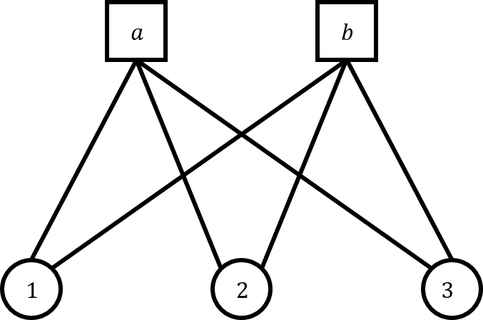
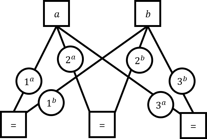
Figure 1: Example of transformation from the factor-graph GM (left) to the Forney-style GM (right). Squares and circles indicate factors and variables respectively. New factors denoted as ‘=’ force adjoining variables be consistent, i.e., have the same value.

2.2 Gauge Transformations

Gauge transformations [19, 20] are a family of linear transformations of the factor functions in (1) which leave the the partition function $Z$ invariant. GTs are defined by the following set of invertible $d\times d$ matrices $\{G_{v\alpha}:(v,\alpha)\in E\}$, termed gauges:

$$G_{v\alpha}=\left[\begin{array}[]{ccc}G_{v\alpha}(1,1)&\cdots&G_{v\alpha}(1,d)\\ \vdots&\ddots&\vdots\\ G_{v\alpha}(d,1)&\cdots&G_{v\alpha}(d,d)\\ \end{array}\right].$$

The transformed GM with respect to the gauges $\mathbf{G}=\{G_{v\alpha}:(v,\alpha)\in E\}$ consists of modified factors $\{\widehat{\mathnormal{f}}_{\alpha}:\alpha\in F\}$ computed as follows:

$$\widehat{\mathnormal{f}}_{\alpha}(\mathbf{x}_{\alpha};\mathbf{G}_{\alpha})=\sum_{\mathbf{x}_{\alpha}^{\prime}}\mathnormal{f}_{\alpha}(\mathbf{x}_{\alpha}^{\prime})\prod_{v\in N(\alpha)}G_{v\alpha}(x_{v},x^{\prime}_{v}),$$ (2)

where $\mathbf{G}_{\alpha}=\{G_{v\alpha}:v\in N(\alpha)\}$. Here, the gauges must satisfy the following gauge constraints:

$$G_{v\alpha}^{\top}G_{v\beta}=\mathbb{I},\qquad\forall v\in X,$$ (3)

where $\mathbb{I}$ is the identity matrix and $N(v)=\{\alpha,\beta\}$ (recall that we assume $|N(v)|=2$). With these constraints, the partition function is known to be invariant under the transformation [19, 20], i.e.,

$$Z~{}=~{}\sum_{\mathbf{x}}\prod_{\alpha\in F}\mathnormal{f}_{\alpha}(\mathbf{x}_{\alpha})~{}=~{}\sum_{\mathbf{x}}\prod_{\alpha\in F}\widehat{\mathnormal{f}}_{\alpha}(\mathbf{x}_{\alpha};\mathbf{G}_{\alpha}).$$

Thus gauges lead to the transformed distribution $p(\mathbf{x};\mathbf{G})=\prod_{\alpha\in F}\widehat{\mathnormal{f}}_{\alpha}(\mathbf{x}_{\alpha};\mathbf{G}_{\alpha})/Z$. We remark that it might be invalid when $\widehat{\mathnormal{f}}_{\alpha}(\mathbf{x}_{\alpha};\mathbf{G}_{\alpha})$ is negative. Nevertheless, even in this case, the partition function invariance still holds. We provide an example of a gauge transformation in the Supplement.

2.3 Weighted Mini-Bucket Elimination

Bucket (or variable) elimination (BE) [31, 32] is a method for computing the partition function exactly based on directly summing out the variables sequentially. First, BE assumes a fixed elimination ordering $o=[v_{1},\cdots,v_{n}]$ among variables nodes $v\in X$. Then BE groups factors by placing each factor $\mathnormal{f}_{\alpha}$ in the “bucket” $B_{v}$ of its earliest argument $v\in N(\alpha)$ appearing in the elimination order $o$. Next, BE eliminates the variable by marginalizing the product of factors in the bucket, i.e.,

$$\mathnormal{f}_{B_{v}}(\mathbf{x}_{B_{v}})=\sum_{x_{v}}\prod_{\mathnormal{f}_{\alpha}\in B_{v}}\mathnormal{f}_{\alpha}(\mathbf{x}_{\alpha})\qquad\forall~{}\mathbf{x}_{B_{v}},$$ (4)

where $\mathbf{x}_{B_{v}}=[x_{u}:u\in var(B_{v}),u\neq v]$ and $var(B_{v})$ indicates the subset of variables in the bucket. Finally, the newly generated function $\mathnormal{f}_{B_{v}}$ is inserted into another bucket corresponding to its earliest argument in the elimination order. This process is easily seen as applying a distributive property: groups of factors corresponding to buckets are summed out sequentially, and then the newly created factor (without the eliminated variable) is assigned to another bucket.

The computational cost of BE is exponential in the number of uneliminated variables in the bucket, i.e., the induced width of the graph given the elimination order. BE is summarized in Algorithm 1.

Algorithm 1 BE for computing $Z$

1:  Input: GM on graph $G=(V,E)$ with $V=(X,F)$ and factors $\mathcal{F}=\{\mathnormal{f}_{\alpha}\}_{\alpha\in F}$ and elimination order $o=[v_{1},\cdots,v_{n}]$.  

2:  $\mathcal{F}^{\prime}\leftarrow\mathcal{F}$

3:  for $v$ in $o$ do

4:     $B_{v}\leftarrow\{\mathnormal{f}_{\alpha}|\mathnormal{f}_{\alpha}\in\mathcal{F},v\in N(\alpha)\}$

5:     Generate new factor by:

$$\mathnormal{f}_{B_{v}}(\mathbf{x}_{B_{v}})=\sum_{x_{v}}\prod_{\mathnormal{f}_{\alpha}\in B_{v}}\mathnormal{f}_{\alpha}(\mathbf{x}_{\alpha}),~{}\forall~{}\mathbf{x}_{B_{v}}.$$

6:     $\mathcal{F}^{\prime}\leftarrow\mathcal{F}^{\prime}\cup\{\mathnormal{f}_{B_{v}}\}-B_{v}$

7:  end for  

8:  Output: $Z=\prod_{\mathnormal{f}_{\alpha}\in\mathcal{F}^{\prime}}\mathnormal{f}_{\alpha}$

Mini-bucket elimination (MBE) [28] and weighted mini-bucket elimination (WMBE) [16] approximate BE by splitting computation of each bucket into several “mini-buckets”, where WMBE additionally makes use of Hölder’s inequality [33]. Since MBE is a special case of WMBE (by choosing extreme Hölder weights), here we focus on providing background for WMBE.

Let $\{\psi_{i}(x),i=1,\cdots,m\}$ be some functions defined on discrete variable $x$, and $\mathbf{w}=[w_{1},\cdots w_{n}]$ be a vector of Hölder weights. We define a weighted absolute summation, defined as follows:

$$\operatorname*{\mathchoice{\ooalign{\phantom{$\displaystyle\sum$}\cr\raisebox{1.2pt}{$\mkern 22.0mu\scalebox{0.7}{$\circ$}$}\cr\raisebox{-0.7pt}{$\mkern 22.0mu\scalebox{0.7}{$\circ$}$}\cr$\displaystyle\sum$}}{\ooalign{$\textstyle\sum$\cr\raisebox{1.9pt}{$\mkern 16.0mu\scalebox{0.4}{$\circ$}$}\cr\raisebox{-0.3pt}{$\mkern 16.0mu\scalebox{0.4}{$\circ$}$}\cr}}{\ooalign{\raisebox{0.0pt}{\scalebox{0.6}{$\scriptstyle\sum$}}\cr\raisebox{1.6pt}{$\mkern 7.5mu\scalebox{0.2}{$\circ$}$}\cr\raisebox{-0.2pt}{$\mkern 7.5mu\scalebox{0.2}{$\circ$}$}\cr}}{\ooalign{\raisebox{0.2pt}{\scalebox{0.6}{$\scriptstyle\sum$}}\cr\raisebox{2.2pt}{$\mkern 7.5mu\scalebox{0.2}{$\circ$}$}\cr\raisebox{0.4pt}{$\mkern 7.5mu\scalebox{0.2}{$\circ$}$}\cr}}}^{w_{i}}_{x}\psi_{i}(x):=\big{(}\sum_{x}|\psi_{i}(x)|^{1/w_{i}}\big{)}^{w_{i}}.$$

Equivalently, $\operatorname*{\mathchoice{\ooalign{\phantom{$\displaystyle\sum$}\cr\raisebox{1.2pt}{$\mkern 22.0mu\scalebox{0.7}{$\circ$}$}\cr\raisebox{-0.7pt}{$\mkern 22.0mu\scalebox{0.7}{$\circ$}$}\cr$\displaystyle\sum$}}{\ooalign{$\textstyle\sum$\cr\raisebox{1.9pt}{$\mkern 16.0mu\scalebox{0.4}{$\circ$}$}\cr\raisebox{-0.3pt}{$\mkern 16.0mu\scalebox{0.4}{$\circ$}$}\cr}}{\ooalign{\raisebox{0.0pt}{\scalebox{0.6}{$\scriptstyle\sum$}}\cr\raisebox{1.6pt}{$\mkern 7.5mu\scalebox{0.2}{$\circ$}$}\cr\raisebox{-0.2pt}{$\mkern 7.5mu\scalebox{0.2}{$\circ$}$}\cr}}{\ooalign{\raisebox{0.2pt}{\scalebox{0.6}{$\scriptstyle\sum$}}\cr\raisebox{2.2pt}{$\mkern 7.5mu\scalebox{0.2}{$\circ$}$}\cr\raisebox{0.4pt}{$\mkern 7.5mu\scalebox{0.2}{$\circ$}$}\cr}}}^{w_{i}}_{x}$ is the Schatten $p$-norm with $p=1/w_{i}$. If $w_{i}>0$ for all $i\geq 1$, then Hölder’s inequality implies that

$$\operatorname*{\mathchoice{\ooalign{\phantom{$\displaystyle\sum$}\cr\raisebox{1.2pt}{$\mkern 22.0mu\scalebox{0.7}{$\circ$}$}\cr\raisebox{-0.7pt}{$\mkern 22.0mu\scalebox{0.7}{$\circ$}$}\cr$\displaystyle\sum$}}{\ooalign{$\textstyle\sum$\cr\raisebox{1.9pt}{$\mkern 16.0mu\scalebox{0.4}{$\circ$}$}\cr\raisebox{-0.3pt}{$\mkern 16.0mu\scalebox{0.4}{$\circ$}$}\cr}}{\ooalign{\raisebox{0.0pt}{\scalebox{0.6}{$\scriptstyle\sum$}}\cr\raisebox{1.6pt}{$\mkern 7.5mu\scalebox{0.2}{$\circ$}$}\cr\raisebox{-0.2pt}{$\mkern 7.5mu\scalebox{0.2}{$\circ$}$}\cr}}{\ooalign{\raisebox{0.2pt}{\scalebox{0.6}{$\scriptstyle\sum$}}\cr\raisebox{2.2pt}{$\mkern 7.5mu\scalebox{0.2}{$\circ$}$}\cr\raisebox{0.4pt}{$\mkern 7.5mu\scalebox{0.2}{$\circ$}$}\cr}}}^{w_{0}}_{x}\prod_{i=1}^{m}\psi_{i}(x)\leq\prod_{i=1}^{m}\operatorname*{\mathchoice{\ooalign{\phantom{$\displaystyle\sum$}\cr\raisebox{1.2pt}{$\mkern 22.0mu\scalebox{0.7}{$\circ$}$}\cr\raisebox{-0.7pt}{$\mkern 22.0mu\scalebox{0.7}{$\circ$}$}\cr$\displaystyle\sum$}}{\ooalign{$\textstyle\sum$\cr\raisebox{1.9pt}{$\mkern 16.0mu\scalebox{0.4}{$\circ$}$}\cr\raisebox{-0.3pt}{$\mkern 16.0mu\scalebox{0.4}{$\circ$}$}\cr}}{\ooalign{\raisebox{0.0pt}{\scalebox{0.6}{$\scriptstyle\sum$}}\cr\raisebox{1.6pt}{$\mkern 7.5mu\scalebox{0.2}{$\circ$}$}\cr\raisebox{-0.2pt}{$\mkern 7.5mu\scalebox{0.2}{$\circ$}$}\cr}}{\ooalign{\raisebox{0.2pt}{\scalebox{0.6}{$\scriptstyle\sum$}}\cr\raisebox{2.2pt}{$\mkern 7.5mu\scalebox{0.2}{$\circ$}$}\cr\raisebox{0.4pt}{$\mkern 7.5mu\scalebox{0.2}{$\circ$}$}\cr}}}^{w_{i}}_{x}\psi_{i}(x),$$ (5)

where $w_{0}=\sum_{i}w_{i}$. If only one weight is positive, e.g., $w_{1}>0$ and $w_{i}<0$ for all $i>1$, we have the reverse Hölder’s inequality:

$$\operatorname*{\mathchoice{\ooalign{\phantom{$\displaystyle\sum$}\cr\raisebox{1.2pt}{$\mkern 22.0mu\scalebox{0.7}{$\circ$}$}\cr\raisebox{-0.7pt}{$\mkern 22.0mu\scalebox{0.7}{$\circ$}$}\cr$\displaystyle\sum$}}{\ooalign{$\textstyle\sum$\cr\raisebox{1.9pt}{$\mkern 16.0mu\scalebox{0.4}{$\circ$}$}\cr\raisebox{-0.3pt}{$\mkern 16.0mu\scalebox{0.4}{$\circ$}$}\cr}}{\ooalign{\raisebox{0.0pt}{\scalebox{0.6}{$\scriptstyle\sum$}}\cr\raisebox{1.6pt}{$\mkern 7.5mu\scalebox{0.2}{$\circ$}$}\cr\raisebox{-0.2pt}{$\mkern 7.5mu\scalebox{0.2}{$\circ$}$}\cr}}{\ooalign{\raisebox{0.2pt}{\scalebox{0.6}{$\scriptstyle\sum$}}\cr\raisebox{2.2pt}{$\mkern 7.5mu\scalebox{0.2}{$\circ$}$}\cr\raisebox{0.4pt}{$\mkern 7.5mu\scalebox{0.2}{$\circ$}$}\cr}}}^{w_{0}}_{x}\prod_{i=1}^{m}\psi_{i}(x)\geq\prod_{i=1}^{m}\operatorname*{\mathchoice{\ooalign{\phantom{$\displaystyle\sum$}\cr\raisebox{1.2pt}{$\mkern 22.0mu\scalebox{0.7}{$\circ$}$}\cr\raisebox{-0.7pt}{$\mkern 22.0mu\scalebox{0.7}{$\circ$}$}\cr$\displaystyle\sum$}}{\ooalign{$\textstyle\sum$\cr\raisebox{1.9pt}{$\mkern 16.0mu\scalebox{0.4}{$\circ$}$}\cr\raisebox{-0.3pt}{$\mkern 16.0mu\scalebox{0.4}{$\circ$}$}\cr}}{\ooalign{\raisebox{0.0pt}{\scalebox{0.6}{$\scriptstyle\sum$}}\cr\raisebox{1.6pt}{$\mkern 7.5mu\scalebox{0.2}{$\circ$}$}\cr\raisebox{-0.2pt}{$\mkern 7.5mu\scalebox{0.2}{$\circ$}$}\cr}}{\ooalign{\raisebox{0.2pt}{\scalebox{0.6}{$\scriptstyle\sum$}}\cr\raisebox{2.2pt}{$\mkern 7.5mu\scalebox{0.2}{$\circ$}$}\cr\raisebox{0.4pt}{$\mkern 7.5mu\scalebox{0.2}{$\circ$}$}\cr}}}^{w_{i}}_{x}\psi_{i}(x).$$ (6)

Algorithm 2 WMBE for bounding $Z$

1:  Input: GM on graph $G=(V,E)$ with $V=(X,F)$, factors $\mathcal{F}=\{\mathnormal{f}_{\alpha}\}_{\alpha\in F}$, elimination order $o=[v_{1},\cdots,v_{n}]$ and bound on bucket size $ibound$.  

2:  $\mathcal{F}^{\prime}\leftarrow\mathcal{F}$

3:  for $v$ in $o$ do

4:     $B_{v}\leftarrow\{\mathnormal{f}_{\alpha}|\mathnormal{f}_{\alpha}\in\mathcal{F}^{\prime},v\in\partial\alpha\}$

5:     Partition $B_{v}$ into $R_{v}$ subgroups $\{B_{v}^{r}\}_{r=1}^{R_{v}}$ such that $|var(B_{v}^{r})|\leq ibound$ for all $r$.

6:     Assign weights $w_{1},\cdots,w_{R_{v}}$ while satisfying $\sum_{r}w_{r}=1$.

7:     for $r\leftarrow 1,\cdots,R_{v}$  do

8:        Generate a new factor by:

$$\mathnormal{f}_{B_{v}^{r}}(\mathbf{x}_{B_{v}^{r}})=\operatorname*{\mathchoice{\ooalign{\phantom{$\displaystyle\sum$}\cr\raisebox{1.2pt}{$\mkern 22.0mu\scalebox{0.7}{$\circ$}$}\cr\raisebox{-0.7pt}{$\mkern 22.0mu\scalebox{0.7}{$\circ$}$}\cr$\displaystyle\sum$}}{\ooalign{$\textstyle\sum$\cr\raisebox{1.9pt}{$\mkern 16.0mu\scalebox{0.4}{$\circ$}$}\cr\raisebox{-0.3pt}{$\mkern 16.0mu\scalebox{0.4}{$\circ$}$}\cr}}{\ooalign{\raisebox{0.0pt}{\scalebox{0.6}{$\scriptstyle\sum$}}\cr\raisebox{1.6pt}{$\mkern 7.5mu\scalebox{0.2}{$\circ$}$}\cr\raisebox{-0.2pt}{$\mkern 7.5mu\scalebox{0.2}{$\circ$}$}\cr}}{\ooalign{\raisebox{0.2pt}{\scalebox{0.6}{$\scriptstyle\sum$}}\cr\raisebox{2.2pt}{$\mkern 7.5mu\scalebox{0.2}{$\circ$}$}\cr\raisebox{0.4pt}{$\mkern 7.5mu\scalebox{0.2}{$\circ$}$}\cr}}}_{x_{v}}^{w_{r}}\prod_{\mathnormal{f}_{\alpha}\in B_{v}^{r}}\mathnormal{f}_{\alpha}(\mathbf{x}_{\alpha}),~{}\forall~{}\mathbf{x}_{B_{v}}.$$

9:        $\mathcal{F}^{\prime}\leftarrow\mathcal{F}^{\prime}\cup\{\mathnormal{f}_{B^{r}_{v}}\}-B_{v}^{r}$

10:     end for

11:  end for  

12:  Output: $Z_{\text{WMBE}}=\prod_{\mathnormal{f}_{\alpha}\in\mathcal{F}^{\prime}}\mathnormal{f}_{\alpha}$

WMBE modifies BE by applying Hölder’s inequality whenever the size of a bucket, i.e., length of $\mathbf{x}_{B_{v}}$, exceeds some given parameter called $ibound$. In this case, WMBE splits the bucket into multiple ‘mini-buckets’, and weighted absolute summation is evaluated sequentially in place of (4), i.e.,

$$\sum_{x_{v}}\prod_{\mathnormal{f}_{\alpha}\in B}|\mathnormal{f}_{\alpha}(\mathbf{x}_{\alpha})|\leq\prod_{r=1}^{R_{v}}\operatorname*{\mathchoice{\ooalign{\phantom{$\displaystyle\sum$}\cr\raisebox{1.2pt}{$\mkern 22.0mu\scalebox{0.7}{$\circ$}$}\cr\raisebox{-0.7pt}{$\mkern 22.0mu\scalebox{0.7}{$\circ$}$}\cr$\displaystyle\sum$}}{\ooalign{$\textstyle\sum$\cr\raisebox{1.9pt}{$\mkern 16.0mu\scalebox{0.4}{$\circ$}$}\cr\raisebox{-0.3pt}{$\mkern 16.0mu\scalebox{0.4}{$\circ$}$}\cr}}{\ooalign{\raisebox{0.0pt}{\scalebox{0.6}{$\scriptstyle\sum$}}\cr\raisebox{1.6pt}{$\mkern 7.5mu\scalebox{0.2}{$\circ$}$}\cr\raisebox{-0.2pt}{$\mkern 7.5mu\scalebox{0.2}{$\circ$}$}\cr}}{\ooalign{\raisebox{0.2pt}{\scalebox{0.6}{$\scriptstyle\sum$}}\cr\raisebox{2.2pt}{$\mkern 7.5mu\scalebox{0.2}{$\circ$}$}\cr\raisebox{0.4pt}{$\mkern 7.5mu\scalebox{0.2}{$\circ$}$}\cr}}}_{x_{v}}^{w_{r}}\prod_{\mathnormal{f}_{\alpha}\in B_{v}^{r}}\mathnormal{f}_{\alpha}(\mathbf{x}_{\alpha}),$$

for all $\mathbf{x}_{B_{v}}$, where Hölder weights satisfy $\sum_{r}w_{r}=1,w_{r}>0$, $B_{v}=\bigcup_{r}B_{v}^{r}$, and $B_{v}^{r}$ is disjoint for all $r$. We then generate multiple new factors by:

$$\mathnormal{f}_{B_{v}^{r}}(\mathbf{x}_{B_{v}^{r}})=\operatorname*{\mathchoice{\ooalign{\phantom{$\displaystyle\sum$}\cr\raisebox{1.2pt}{$\mkern 22.0mu\scalebox{0.7}{$\circ$}$}\cr\raisebox{-0.7pt}{$\mkern 22.0mu\scalebox{0.7}{$\circ$}$}\cr$\displaystyle\sum$}}{\ooalign{$\textstyle\sum$\cr\raisebox{1.9pt}{$\mkern 16.0mu\scalebox{0.4}{$\circ$}$}\cr\raisebox{-0.3pt}{$\mkern 16.0mu\scalebox{0.4}{$\circ$}$}\cr}}{\ooalign{\raisebox{0.0pt}{\scalebox{0.6}{$\scriptstyle\sum$}}\cr\raisebox{1.6pt}{$\mkern 7.5mu\scalebox{0.2}{$\circ$}$}\cr\raisebox{-0.2pt}{$\mkern 7.5mu\scalebox{0.2}{$\circ$}$}\cr}}{\ooalign{\raisebox{0.2pt}{\scalebox{0.6}{$\scriptstyle\sum$}}\cr\raisebox{2.2pt}{$\mkern 7.5mu\scalebox{0.2}{$\circ$}$}\cr\raisebox{0.4pt}{$\mkern 7.5mu\scalebox{0.2}{$\circ$}$}\cr}}}_{x_{v}}^{w_{r}}\prod_{\mathnormal{f}_{\alpha}\in B_{v}^{r}}\mathnormal{f}_{\alpha}(\mathbf{x}_{\alpha}),\qquad\forall~{}\mathbf{x}_{B_{v}},$$

and insert into other buckets. By construction, WMBE yields an upper bound for the partition function $Z$. One can use the same idea to derive a lower bound for $Z$ using the reverse Hölder’s inequality. We summarize WMBE in Algorithm 2.

One can interpret MBE as a special case of WMBE by assigning a single weight to be close to $1$ and others to be close to $0$, i.e., $\mathbf{w}=\lim_{w\rightarrow 0^{+}}[1-w,w,w,\cdots]$. Instead, Liu and Ihler [16] optimize the Hölder weights so that WMBE can outperform MBE, which we discuss further in Section 3.

3 GAUGED WMBE ALGORITHM

In this section, we describe our gauge optimization scheme WMBE-G to improve the previous WMBE bound, yielding gauranteed upper bound approximations for the partition function $Z$. Our scheme improves the standard WMBE bound by searching over the large family of gauge transformed (possibly invalid) GMs to find the tightest WMBE bound possible.

3.1 Key Optimization Formulation

In order to describe the optimization formulation for tightening the WMBE bound, we first observe that (8) can be reformulated into

$$\sum_{x_{v}}\prod_{\mathnormal{f}_{\alpha}\in B}|\mathnormal{f}_{\alpha}(\mathbf{x}_{\alpha})|\leq\sum_{x_{v}^{(1)}}^{w_{1}}\cdots\operatorname*{\mathchoice{\ooalign{\phantom{$\displaystyle\sum$}\cr\raisebox{1.2pt}{$\mkern 22.0mu\scalebox{0.7}{$\circ$}$}\cr\raisebox{-0.7pt}{$\mkern 22.0mu\scalebox{0.7}{$\circ$}$}\cr$\displaystyle\sum$}}{\ooalign{$\textstyle\sum$\cr\raisebox{1.9pt}{$\mkern 16.0mu\scalebox{0.4}{$\circ$}$}\cr\raisebox{-0.3pt}{$\mkern 16.0mu\scalebox{0.4}{$\circ$}$}\cr}}{\ooalign{\raisebox{0.0pt}{\scalebox{0.6}{$\scriptstyle\sum$}}\cr\raisebox{1.6pt}{$\mkern 7.5mu\scalebox{0.2}{$\circ$}$}\cr\raisebox{-0.2pt}{$\mkern 7.5mu\scalebox{0.2}{$\circ$}$}\cr}}{\ooalign{\raisebox{0.2pt}{\scalebox{0.6}{$\scriptstyle\sum$}}\cr\raisebox{2.2pt}{$\mkern 7.5mu\scalebox{0.2}{$\circ$}$}\cr\raisebox{0.4pt}{$\mkern 7.5mu\scalebox{0.2}{$\circ$}$}\cr}}}_{x_{v}^{(R_{v})}}^{w_{R_{v}}}\prod_{r=1}^{R_{v}}\prod_{\alpha\in B_{v}^{r}}\mathnormal{f}_{\alpha}(\mathbf{x}_{\alpha\backslash v},x_{v}^{(r)})$$ (7)

where $\mathbf{x}_{\alpha\backslash v}=[x_{u}:u\in N(\alpha),u\neq v]$. While notation is complex, this is simply applying the distributive property on the right hand side of (8). The procedure can be seen as ‘splitting’ variable from $x_{v}$ to $x_{v}^{(1)},\cdots x_{v}^{(R_{v})}$ and its associated node from $v$ to $v^{(1)},\cdots v^{(R_{v})}$ so that factors no longer share the split variable. We remark that under Forney-style GMs, $R_{v}\leq 2$ since exactly $2$ factors are associated with a variable. After repeatedly applying the inequality, we arrive at the following WMBE bound, termed weighted partition function:

$$Z\leq Z_{\text{WMBE}}=\operatorname*{\mathchoice{\ooalign{\phantom{$\displaystyle\sum$}\cr\raisebox{1.2pt}{$\mkern 22.0mu\scalebox{0.7}{$\circ$}$}\cr\raisebox{-0.7pt}{$\mkern 22.0mu\scalebox{0.7}{$\circ$}$}\cr$\displaystyle\sum$}}{\ooalign{$\textstyle\sum$\cr\raisebox{1.9pt}{$\mkern 16.0mu\scalebox{0.4}{$\circ$}$}\cr\raisebox{-0.3pt}{$\mkern 16.0mu\scalebox{0.4}{$\circ$}$}\cr}}{\ooalign{\raisebox{0.0pt}{\scalebox{0.6}{$\scriptstyle\sum$}}\cr\raisebox{1.6pt}{$\mkern 7.5mu\scalebox{0.2}{$\circ$}$}\cr\raisebox{-0.2pt}{$\mkern 7.5mu\scalebox{0.2}{$\circ$}$}\cr}}{\ooalign{\raisebox{0.2pt}{\scalebox{0.6}{$\scriptstyle\sum$}}\cr\raisebox{2.2pt}{$\mkern 7.5mu\scalebox{0.2}{$\circ$}$}\cr\raisebox{0.4pt}{$\mkern 7.5mu\scalebox{0.2}{$\circ$}$}\cr}}}^{\bar{w}_{\bar{n}}}_{\bar{x}_{\bar{1}}}\cdots\operatorname*{\mathchoice{\ooalign{\phantom{$\displaystyle\sum$}\cr\raisebox{1.2pt}{$\mkern 22.0mu\scalebox{0.7}{$\circ$}$}\cr\raisebox{-0.7pt}{$\mkern 22.0mu\scalebox{0.7}{$\circ$}$}\cr$\displaystyle\sum$}}{\ooalign{$\textstyle\sum$\cr\raisebox{1.9pt}{$\mkern 16.0mu\scalebox{0.4}{$\circ$}$}\cr\raisebox{-0.3pt}{$\mkern 16.0mu\scalebox{0.4}{$\circ$}$}\cr}}{\ooalign{\raisebox{0.0pt}{\scalebox{0.6}{$\scriptstyle\sum$}}\cr\raisebox{1.6pt}{$\mkern 7.5mu\scalebox{0.2}{$\circ$}$}\cr\raisebox{-0.2pt}{$\mkern 7.5mu\scalebox{0.2}{$\circ$}$}\cr}}{\ooalign{\raisebox{0.2pt}{\scalebox{0.6}{$\scriptstyle\sum$}}\cr\raisebox{2.2pt}{$\mkern 7.5mu\scalebox{0.2}{$\circ$}$}\cr\raisebox{0.4pt}{$\mkern 7.5mu\scalebox{0.2}{$\circ$}$}\cr}}}^{\bar{w}_{1}}_{\bar{x}_{1}}\prod_{\alpha\in F}\mathnormal{f}_{\alpha}(\bar{\mathbf{x}}_{\alpha}).$$ (8)

In (8), $\bar{\mathbf{x}}=[\bar{x}_{1},\cdots,\bar{x}_{\bar{n}}]$ and $\bar{\mathbf{w}}=[\bar{w}_{1},\cdots,\bar{x}_{\bar{n}}]$ indicate the ‘split’ version of variables and associated Hölder weights, indexed by appearance of associated node in the modified elimination order $\bar{o}=[v_{1}^{(1)},\cdots v_{1}^{(R_{v_{1}})},\cdots,v_{n}^{(1)},\cdots v_{n}^{(R_{v_{n}})}]$. Therefore, the WMBE bound can be seen as a weighted absolute summation over product of factors in a new GM. However, unlike the original partition function, the weighted absolute summation is tractable with respect to $ibound$ since at most $d^{ibound}$ terms are counted for each weighted absolute summation, or equivalently variable elimination of mini-buckets. Finally, we are able to present our main optimization formulation:

$$\operatornamewithlimits{\mbox{minimize}}_{\mathbf{G}}\quad \operatorname*{\mathchoice{\ooalign{\phantom{$\displaystyle\sum$}\cr\raisebox{1.2pt}{$\mkern 22.0mu\scalebox{0.7}{$\circ$}$}\cr\raisebox{-0.7pt}{$\mkern 22.0mu\scalebox{0.7}{$\circ$}$}\cr$\displaystyle\sum$}}{\ooalign{$\textstyle\sum$\cr\raisebox{1.9pt}{$\mkern 16.0mu\scalebox{0.4}{$\circ$}$}\cr\raisebox{-0.3pt}{$\mkern 16.0mu\scalebox{0.4}{$\circ$}$}\cr}}{\ooalign{\raisebox{0.0pt}{\scalebox{0.6}{$\scriptstyle\sum$}}\cr\raisebox{1.6pt}{$\mkern 7.5mu\scalebox{0.2}{$\circ$}$}\cr\raisebox{-0.2pt}{$\mkern 7.5mu\scalebox{0.2}{$\circ$}$}\cr}}{\ooalign{\raisebox{0.2pt}{\scalebox{0.6}{$\scriptstyle\sum$}}\cr\raisebox{2.2pt}{$\mkern 7.5mu\scalebox{0.2}{$\circ$}$}\cr\raisebox{0.4pt}{$\mkern 7.5mu\scalebox{0.2}{$\circ$}$}\cr}}}^{\bar{w}_{\bar{n}}}_{\bar{x}_{\bar{n}}}\cdots\operatorname*{\mathchoice{\ooalign{\phantom{$\displaystyle\sum$}\cr\raisebox{1.2pt}{$\mkern 22.0mu\scalebox{0.7}{$\circ$}$}\cr\raisebox{-0.7pt}{$\mkern 22.0mu\scalebox{0.7}{$\circ$}$}\cr$\displaystyle\sum$}}{\ooalign{$\textstyle\sum$\cr\raisebox{1.9pt}{$\mkern 16.0mu\scalebox{0.4}{$\circ$}$}\cr\raisebox{-0.3pt}{$\mkern 16.0mu\scalebox{0.4}{$\circ$}$}\cr}}{\ooalign{\raisebox{0.0pt}{\scalebox{0.6}{$\scriptstyle\sum$}}\cr\raisebox{1.6pt}{$\mkern 7.5mu\scalebox{0.2}{$\circ$}$}\cr\raisebox{-0.2pt}{$\mkern 7.5mu\scalebox{0.2}{$\circ$}$}\cr}}{\ooalign{\raisebox{0.2pt}{\scalebox{0.6}{$\scriptstyle\sum$}}\cr\raisebox{2.2pt}{$\mkern 7.5mu\scalebox{0.2}{$\circ$}$}\cr\raisebox{0.4pt}{$\mkern 7.5mu\scalebox{0.2}{$\circ$}$}\cr}}}^{\bar{w}_{1}}_{\bar{x}_{1}}\prod_{\alpha\in F}\widehat{\mathnormal{f}}_{\alpha}(\bar{\mathbf{x}}_{\alpha};\mathbf{G}_{\alpha}),$$ (35)

subject to $$G_{v\alpha}^{\top}G_{v\beta}=\mathbb{I},\quad\forall~{}v\in X,N(v)=\{\alpha,\beta\}.$$

3.2 Algorithm Description

We now describe an efficient algorithm to optimize (35). First, the gauge constraint can be removed simply by expressing one (of the two) gauges in terms of the other, e.g., $G_{v\beta}$ via $(G_{v\alpha}^{\top})^{-1}$. Then, (35) can be optimized via any type of unconstrained optimization solver. Here, we optimize gauges by gradient descent followed by additional updates on factor values.

To this end, we initialize gauges by identity matrices, which immediately yields the original WMBE bound from (8) since $\mathnormal{f}_{\alpha}(\mathbf{x}_{\alpha})=\widehat{\mathnormal{f}}_{\alpha}(\mathbf{x}_{\alpha};\mathbb{I}_{\alpha})$, where $\mathbb{I}_{\alpha}=[G_{v\alpha}=\mathbb{I}:(v,\alpha)\in E]$. Next, under expressing gauges via one another, i.e., $G_{v\beta}\leftarrow\left(G_{v\alpha}^{\top}\right)^{-1}$, we update each gauge element by gradient descent for minimization of the weighted $\log$ partition function upper bound $\log Z_{\text{WMBE}}$ as follows:

$$G_{v\alpha}(x_{v}^{\prime},x_{v}^{\prime\prime})~{}\leftarrow~{} G_{v\alpha}(x_{v}^{\prime},x_{v}^{\prime\prime})-\mu\frac{\partial\log Z_{\text{WMBE}}}{\partial G_{v\alpha}(x_{v}^{\prime},x_{v}^{\prime\prime})}$$

$$\frac{\partial\log Z_{\text{WMBE}}}{\partial G_{v\alpha}(x_{v}^{\prime},x_{v}^{\prime\prime})}~{}=~{} \sum_{\bar{\mathbf{x}}_{\alpha\backslash v}}q(\bar{\mathbf{x}}_{\alpha\backslash v},x_{v}^{\prime\prime})\frac{\mathnormal{f}_{\alpha}(\bar{\mathbf{x}}_{\alpha\backslash v},x_{v}^{\prime})}{\mathnormal{f}_{\alpha}(\bar{\mathbf{x}}_{\alpha\backslash v},x_{v}^{\prime\prime})}$$

$$\-\!\!\!\!\!\!-\sum_{\bar{\mathbf{x}}_{\beta\backslash v}}q(\bar{\mathbf{x}}_{\beta\backslash v},x_{v}^{\prime})\frac{\mathnormal{f}_{\beta}(\bar{\mathbf{x}}_{\beta\backslash v},x_{v}^{\prime\prime})}{\mathnormal{f}_{\beta}(\bar{\mathbf{x}}_{\beta\backslash v},x_{v}^{\prime})},$$ (36)

where $\mu$ is the step size, $\mathbf{x}_{\alpha\backslash v}=[x_{u}:u\in N(\alpha),u\neq v]$ and $q$ is an ‘auxiliary distribution’ defined as

$$q(\bar{\mathbf{x}}) =\prod_{k=1}^{\bar{n}}q(\bar{x}_{k}|\bar{x}_{k+1:\bar{n}}),$$

$$q(\bar{x}_{k}|\bar{x}_{k+1:n}) \propto\left(\operatorname*{\mathchoice{\ooalign{\phantom{$\displaystyle\sum$}\cr\raisebox{1.2pt}{$\mkern 22.0mu\scalebox{0.7}{$\circ$}$}\cr\raisebox{-0.7pt}{$\mkern 22.0mu\scalebox{0.7}{$\circ$}$}\cr$\displaystyle\sum$}}{\ooalign{$\textstyle\sum$\cr\raisebox{1.9pt}{$\mkern 16.0mu\scalebox{0.4}{$\circ$}$}\cr\raisebox{-0.3pt}{$\mkern 16.0mu\scalebox{0.4}{$\circ$}$}\cr}}{\ooalign{\raisebox{0.0pt}{\scalebox{0.6}{$\scriptstyle\sum$}}\cr\raisebox{1.6pt}{$\mkern 7.5mu\scalebox{0.2}{$\circ$}$}\cr\raisebox{-0.2pt}{$\mkern 7.5mu\scalebox{0.2}{$\circ$}$}\cr}}{\ooalign{\raisebox{0.2pt}{\scalebox{0.6}{$\scriptstyle\sum$}}\cr\raisebox{2.2pt}{$\mkern 7.5mu\scalebox{0.2}{$\circ$}$}\cr\raisebox{0.4pt}{$\mkern 7.5mu\scalebox{0.2}{$\circ$}$}\cr}}}_{\bar{x}_{k-1}}^{\bar{w}_{k-1}}\cdots\operatorname*{\mathchoice{\ooalign{\phantom{$\displaystyle\sum$}\cr\raisebox{1.2pt}{$\mkern 22.0mu\scalebox{0.7}{$\circ$}$}\cr\raisebox{-0.7pt}{$\mkern 22.0mu\scalebox{0.7}{$\circ$}$}\cr$\displaystyle\sum$}}{\ooalign{$\textstyle\sum$\cr\raisebox{1.9pt}{$\mkern 16.0mu\scalebox{0.4}{$\circ$}$}\cr\raisebox{-0.3pt}{$\mkern 16.0mu\scalebox{0.4}{$\circ$}$}\cr}}{\ooalign{\raisebox{0.0pt}{\scalebox{0.6}{$\scriptstyle\sum$}}\cr\raisebox{1.6pt}{$\mkern 7.5mu\scalebox{0.2}{$\circ$}$}\cr\raisebox{-0.2pt}{$\mkern 7.5mu\scalebox{0.2}{$\circ$}$}\cr}}{\ooalign{\raisebox{0.2pt}{\scalebox{0.6}{$\scriptstyle\sum$}}\cr\raisebox{2.2pt}{$\mkern 7.5mu\scalebox{0.2}{$\circ$}$}\cr\raisebox{0.4pt}{$\mkern 7.5mu\scalebox{0.2}{$\circ$}$}\cr}}}_{\bar{x}_{1}}^{\bar{w}_{1}}\prod_{\alpha\in F}\mathnormal{f}_{\alpha}(\bar{\mathbf{x}}_{\alpha})\right)^{1/\bar{w}_{k}}.$$

We also update $G_{v\beta}\leftarrow(G_{v\alpha}^{\top})^{-1}$ and the value of associated factors by the gauge-transformed factors, i.e.,

$$\mathnormal{f}_{\alpha}(\mathbf{x}_{\alpha})\leftarrow\widehat{\mathnormal{f}}_{\alpha}(\mathbf{x}_{\alpha};\mathbf{G}_{\alpha}),$$ (37)

and similarly for $\mathnormal{f}_{\beta}$. Finally, for the next iteration, we reset $G_{v\alpha}\leftarrow\mathbb{I}$.

The above update leads to an improved WMBE bound, which can be repeated for better bounds (until convergence). Each iteration $t=1,\dots T$ results in a sequence of gauges $\mathbf{G}^{(t)}$ obtained by (3.2), and factors $\mathnormal{f}^{(t)}_{\alpha}$ obtained by (37) can be expressed as $\mathnormal{f}^{(t)}_{\alpha}(\mathbf{x}_{\alpha})=\widehat{\mathnormal{f}}^{(0)}_{\alpha}(\mathbf{x}_{\alpha};\mathbf{G}_{\alpha}^{\prime}),$ where $\mathnormal{f}^{(0)}_{\alpha}=\mathnormal{f}_{\alpha}$ is the original GM factor, and $\mathbf{G}_{\alpha}^{\prime}$ consists of gauges $G_{v\alpha}^{\prime}=G_{v\alpha}^{(t+1)}G_{v\alpha}^{(t)}\cdots G_{v\alpha}^{(1)}$ for $v\in N(\alpha)$. We remark that one can use naïve gradient descent, i.e., update gauges only (without resetting to identity matrices), instead of factors as in (37). However, by utilizing the additional factor updates, the gradient formulation is simplified and redundant computations of gauge transformations are reduced. We summarize the above update procedure in Algorithm 3.

Furthermore, one can utilize ideas from [16] in order to improve the efficiency and power of the proposed optimization. First, computation of auxiliary marginals $q(\mathbf{x}_{\alpha})$ in (3.2) can be efficiently carried out by a message-passing scheme proposed by the authors. Moreover, one can jointly optimize the Hölder weights $\bar{\mathbf{w}}$ in addition to $\mathbf{G}$ using the auxiliary distribution during optimization of (35). In our experiments, we utilize both the message-passing algorithm and the joint optimization involving $\bar{\mathbf{w}}$ using the log-gradient step proposed by the authors.

Finally, we remark that the elimination order and bucket split strategy might be another freedom that one may exploit in order to tighten the WMBE bound. However, their optimizations are hard (see [16]). Hence, we choose the elimination order arbitrarily in our experiments. For the bucket split strategy, if one assumes Forney-style GMs, any strategy reduces into a fixed split process, i.e., whenever $ibound$ is exceeded, a variable $x$ is always split in two parts $x^{(1)},x^{(2)}$, and adjacent factors are assigned separately.

Algorithm 3 Gauged WMBE for bounding $Z$

1:  Input: GM on graph $G=(V,E)$ with $V=(X,F)$, factors $\mathcal{F}=\{\mathnormal{f}_{\alpha}\}_{\alpha\in F}$, elimination order $o=[v_{1},\cdots,v_{n}]$ and bound on bucket size $ibound$.  

2:  $\mathcal{F}^{\prime}\leftarrow\mathcal{F}$

3:  $\bar{o}\leftarrow\emptyset,\bar{w}\leftarrow\emptyset$.

4:  Initialize by $\bar{o}=\emptyset,\bar{\mathbf{w}}=\emptyset$.

5:  for $v$ in $o$ do

6:     $B_{v}\leftarrow\{\mathnormal{f}_{\alpha}|\mathnormal{f}_{\alpha}\in\mathcal{F}^{\prime},v\in N(\alpha)\}$

7:     Partition $B_{v}$ into $R_{v}$ subgroups $\{B_{v}^{r}\}_{r=1}^{R_{v}}$ such that $|var(B_{v}^{r})|\leq ibound$ for all $r$.

8:     Assign weights $w_{1},\cdots,w_{R_{v}}$ while satisfying $\sum_{r}w_{r}=1$.

9:     for $r\leftarrow 1,\cdots,R_{v}$  do

10:        Generate a new factor by:

$$\mathnormal{f}_{B_{v}^{r}}(\mathbf{x}_{B_{v}^{r}})=\operatorname*{\mathchoice{\ooalign{\phantom{$\displaystyle\sum$}\cr\raisebox{1.2pt}{$\mkern 22.0mu\scalebox{0.7}{$\circ$}$}\cr\raisebox{-0.7pt}{$\mkern 22.0mu\scalebox{0.7}{$\circ$}$}\cr$\displaystyle\sum$}}{\ooalign{$\textstyle\sum$\cr\raisebox{1.9pt}{$\mkern 16.0mu\scalebox{0.4}{$\circ$}$}\cr\raisebox{-0.3pt}{$\mkern 16.0mu\scalebox{0.4}{$\circ$}$}\cr}}{\ooalign{\raisebox{0.0pt}{\scalebox{0.6}{$\scriptstyle\sum$}}\cr\raisebox{1.6pt}{$\mkern 7.5mu\scalebox{0.2}{$\circ$}$}\cr\raisebox{-0.2pt}{$\mkern 7.5mu\scalebox{0.2}{$\circ$}$}\cr}}{\ooalign{\raisebox{0.2pt}{\scalebox{0.6}{$\scriptstyle\sum$}}\cr\raisebox{2.2pt}{$\mkern 7.5mu\scalebox{0.2}{$\circ$}$}\cr\raisebox{0.4pt}{$\mkern 7.5mu\scalebox{0.2}{$\circ$}$}\cr}}}_{x_{v}}^{w_{r}}\prod_{\mathnormal{f}_{\alpha}\in B_{v}^{r}}\mathnormal{f}_{\alpha}(\mathbf{x}_{\alpha}),~{}\forall~{}\mathbf{x}_{B_{v}}.$$

11:        $\mathcal{F}^{\prime}\leftarrow\mathcal{F}^{\prime}\cup\{\mathnormal{f}_{B^{r}_{v}}\}-B_{v}^{r}$

12:     end for

13:     Extend $\bar{o}$ by $[v^{(1)},\cdots,v^{(R_{v})}]$

14:     Extend $\bar{\mathbf{w}}$ by $[w_{1},\cdots,w_{R_{v}}]$

15:  end for

16:  Initialize by $G_{v\alpha}=\mathbb{I}$ for all $(v,\alpha)\in E$.

17:  for $t=1,2,\cdots,T$ do

18:     for $v$ in $X$ with $N(v)=\{\alpha,\beta\}$ do

19:        Update $G_{v\alpha}$ by (3.2).

20:        $G_{v\beta}\leftarrow(G_{v\alpha}^{\top})^{-1}$

21:        Set $\mathnormal{f}_{\alpha}(\mathbf{x}_{\alpha})\leftarrow\widehat{\mathnormal{f}}_{\alpha}(\mathbf{x}_{\alpha};\mathbf{G}_{\alpha})$ and $\mathnormal{f}_{\alpha}(\mathbf{x}_{\alpha})\leftarrow\widehat{\mathnormal{f}}_{\alpha}(\mathbf{x}_{\alpha};\mathbf{G}_{\alpha})$ for all $\mathbf{x}_{\alpha}$, $\mathbf{x}_{\beta}$.

22:        Reset gauges $G_{v\alpha},G_{v\beta}\leftarrow\mathbb{I}$.

23:     end for

24:  end for  

25:  Output: $Z_{\text{WMBE-G}}=\prod_{\mathnormal{f}^{\prime}\in\mathcal{F}^{\prime}}\mathnormal{f}$

3.3 Relation to Previous Work

Hölder’s inequality holds even for negative-valued functions, so we do not need to put any additional constraint on non-negativity of factors, e.g., $\widehat{\mathnormal{f}}_{\alpha}(\bar{\mathbf{x}}_{\alpha};\mathbf{G}_{\alpha})\geq 0$. Thus, invalid gauged transformed GMs are allowed for (35). This contrasts with the earlier work of [26], where additional non-negativity constraints were needed to restrict the gauge transformations considered. Consequently, to our knowledge, our formulation is the first to explore the full range of freedom in gauge transformations when combined with methods of variational inference for GMs. Further, avoiding these non-negativity constraints simplifies our optimization procedure enabling an approach which scales much better than that of [26].

We emphasize that our optimization formulation (35) is a strict generalization of the approach of [16] which optimizes the WMBE bound with respect to reparameterization of GMs. Specifically, the GM reparameterized with respect to reparameterization parameters $\boldsymbol{\theta}=[\theta_{v\alpha}:(v,\alpha)\in E]$ consists of factors:

$$\widehat{\mathnormal{f}}_{\alpha}(\mathbf{x}_{\alpha};\boldsymbol{\theta}_{\alpha})=\prod_{v\in N(\alpha)}\exp(\theta_{v\alpha}(x_{i}))\mathnormal{f}_{\alpha}(\mathbf{x}_{\alpha}),$$ (38)

where $\boldsymbol{\theta}_{\alpha}=\{\theta_{v\alpha}:v\in N(\alpha)\}$. Here, the reparameterization parameter $\theta_{v\alpha}$ is constrained to satisfy the following constraint:

$$\exp(\theta_{v\alpha}(x_{v})+\theta_{v\beta}(x_{v}))=1\quad\forall~{}v\in X,x_{v},$$ (39)

where $N(v)=\{\alpha,\beta\}$. With this constraint, it is easy to check that such transformations are distribution-invariant [18] and form a strict subset of gauge transformations. Alternatively, when gauges are restricted to diagonal matrices with non-negative elements, (2) and (3) match (38) and (39), respectively. Therefore, optimizing (35) is guaranteed to perform no worse than that of [16]. Formally, we provide the following analytic class of GMs where gauge transformations are expected to perform strictly better than reparameterizations. Here, we say a function of binary variables is symmetric if its value is invariant under a ‘flipping’ of all variables in its scope, e.g., $\mathnormal{f}_{\alpha}(2,1,2)=\mathnormal{f}_{\alpha}(1,2,1)$.

Theorem 1.

Consider a GM over binary variables (i.e., $d=2$) where every factor $\mathnormal{f}_{\alpha}$ is symmetric. Then, $\boldsymbol{\theta}=\{\theta_{v\alpha}(x_{v})=0,~{}\forall(v,\alpha)\in E,x_{v}\}$ is always a solution of the following optimization:

$$\operatornamewithlimits{\mbox{minimize}}_{\boldsymbol{\theta}}\quad \operatorname*{\mathchoice{\ooalign{\phantom{$\displaystyle\sum$}\cr\raisebox{1.2pt}{$\mkern 22.0mu\scalebox{0.7}{$\circ$}$}\cr\raisebox{-0.7pt}{$\mkern 22.0mu\scalebox{0.7}{$\circ$}$}\cr$\displaystyle\sum$}}{\ooalign{$\textstyle\sum$\cr\raisebox{1.9pt}{$\mkern 16.0mu\scalebox{0.4}{$\circ$}$}\cr\raisebox{-0.3pt}{$\mkern 16.0mu\scalebox{0.4}{$\circ$}$}\cr}}{\ooalign{\raisebox{0.0pt}{\scalebox{0.6}{$\scriptstyle\sum$}}\cr\raisebox{1.6pt}{$\mkern 7.5mu\scalebox{0.2}{$\circ$}$}\cr\raisebox{-0.2pt}{$\mkern 7.5mu\scalebox{0.2}{$\circ$}$}\cr}}{\ooalign{\raisebox{0.2pt}{\scalebox{0.6}{$\scriptstyle\sum$}}\cr\raisebox{2.2pt}{$\mkern 7.5mu\scalebox{0.2}{$\circ$}$}\cr\raisebox{0.4pt}{$\mkern 7.5mu\scalebox{0.2}{$\circ$}$}\cr}}}^{\bar{w}_{\bar{n}}}_{\bar{x}_{\bar{1}}}\cdots\operatorname*{\mathchoice{\ooalign{\phantom{$\displaystyle\sum$}\cr\raisebox{1.2pt}{$\mkern 22.0mu\scalebox{0.7}{$\circ$}$}\cr\raisebox{-0.7pt}{$\mkern 22.0mu\scalebox{0.7}{$\circ$}$}\cr$\displaystyle\sum$}}{\ooalign{$\textstyle\sum$\cr\raisebox{1.9pt}{$\mkern 16.0mu\scalebox{0.4}{$\circ$}$}\cr\raisebox{-0.3pt}{$\mkern 16.0mu\scalebox{0.4}{$\circ$}$}\cr}}{\ooalign{\raisebox{0.0pt}{\scalebox{0.6}{$\scriptstyle\sum$}}\cr\raisebox{1.6pt}{$\mkern 7.5mu\scalebox{0.2}{$\circ$}$}\cr\raisebox{-0.2pt}{$\mkern 7.5mu\scalebox{0.2}{$\circ$}$}\cr}}{\ooalign{\raisebox{0.2pt}{\scalebox{0.6}{$\scriptstyle\sum$}}\cr\raisebox{2.2pt}{$\mkern 7.5mu\scalebox{0.2}{$\circ$}$}\cr\raisebox{0.4pt}{$\mkern 7.5mu\scalebox{0.2}{$\circ$}$}\cr}}}^{\bar{w}_{1}}_{\bar{x}_{1}}\prod_{\alpha\in F}\widehat{\mathnormal{f}}_{\alpha}(\bar{\mathbf{x}}_{\alpha};\boldsymbol{\theta}_{\alpha}),$$

subject to $$\exp(\theta_{v\alpha}(x_{v})+\theta_{v\beta}(x_{v}))=1\quad\forall~{}v\in X,x_{v}.$$

The proof of Theorem 1 is given in the Supplement. It shows that for symmetric GMs, e.g., the Ising model with no magnetic field, reparameterization is impossible to improve the WMBE bound. On the other hand, gauges are expected to improve it as we explain in what follows. We first remark that the optimality condition for reparameterization is equivalent to the zero gradient condition for diagonal elements of gauges, i.e., $\sum_{\bar{\mathbf{x}}_{\alpha\backslash v}}q(\bar{\mathbf{x}}_{\alpha})=\sum_{\bar{\mathbf{x}}_{\beta\backslash v}}q(\bar{\mathbf{x}}_{\beta})$, which aims to match the auxiliary marginals of variables split by WMBE. Under symmetric models, variables are indistinguishable from an auxiliary marginals point of view, which leads to Theorem 1. On the other hand, the zero gradient condition for non-diagonal gauges is harder to match since it takes local conditional dependency into account, e.g., considers $\mathnormal{f}_{\alpha}(\bar{\mathbf{x}}_{\alpha\backslash v},x_{v}^{\prime})/\mathnormal{f}_{\alpha}(\bar{\mathbf{x}}_{\alpha\backslash v},x_{v}^{\prime\prime})$ upon evaluating the gradient. For symmetric GMs, the above reasoning for reparameterization fails since variables are distinguishable after conditioning, e.g., $\mathnormal{f}_{\alpha}(\bar{\mathbf{x}}_{\alpha\backslash v},x_{v}^{\prime})\neq\mathnormal{f}_{\alpha}(\bar{\mathbf{x}}_{\alpha\backslash v},x_{v}^{\prime\prime})$. Namely, optimal gauges believably have non-diagonal elements. Indeed, in all our experiments, gauge transformations significantly outperform reparameterizations.

4 EXPERIMENTS

In this section, we report experimental results on performance of our proposed algorithms for the task of upper bounding the partition function $Z$.

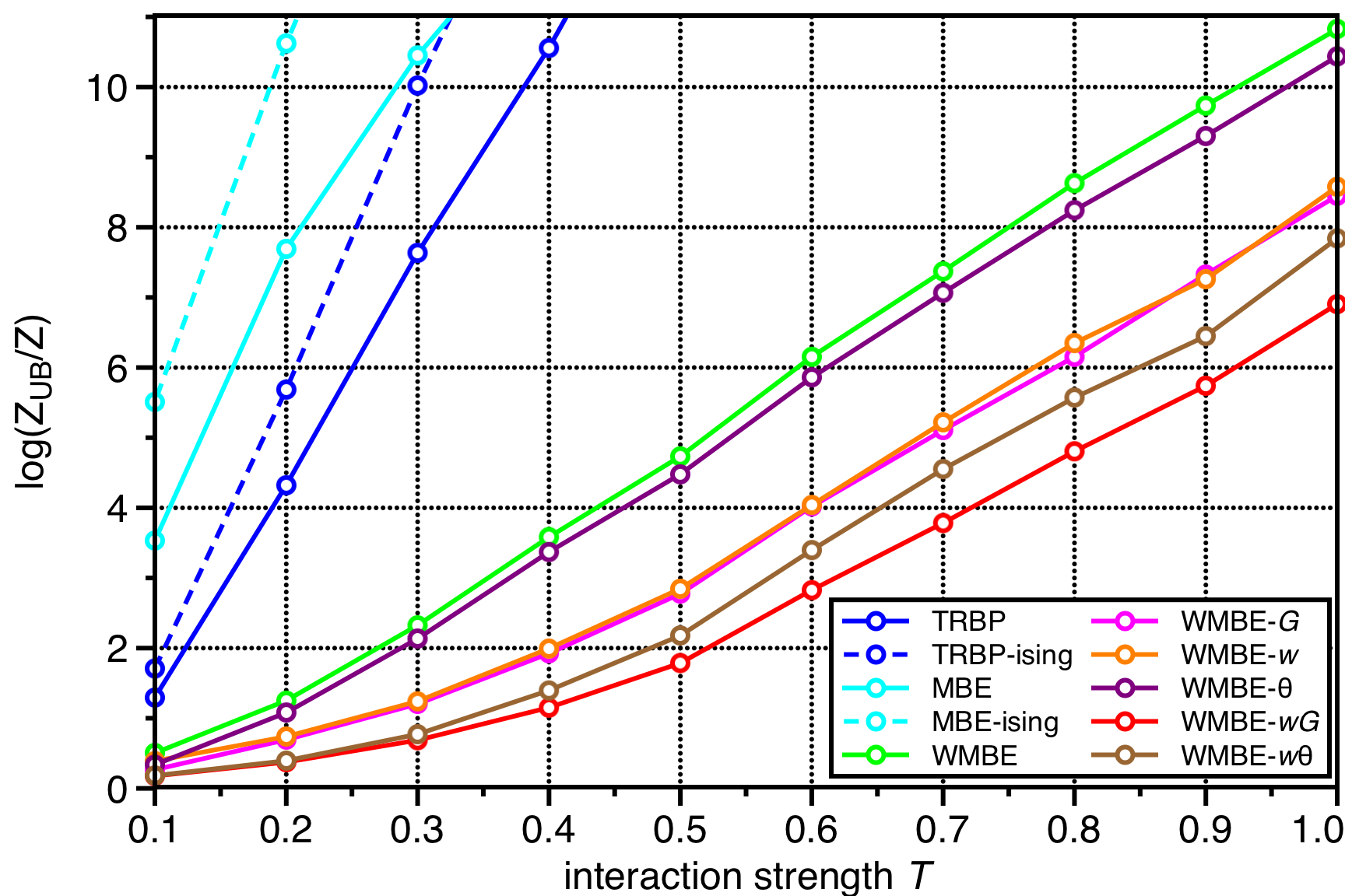
(a) Ising grid GMs, $ibound=4$

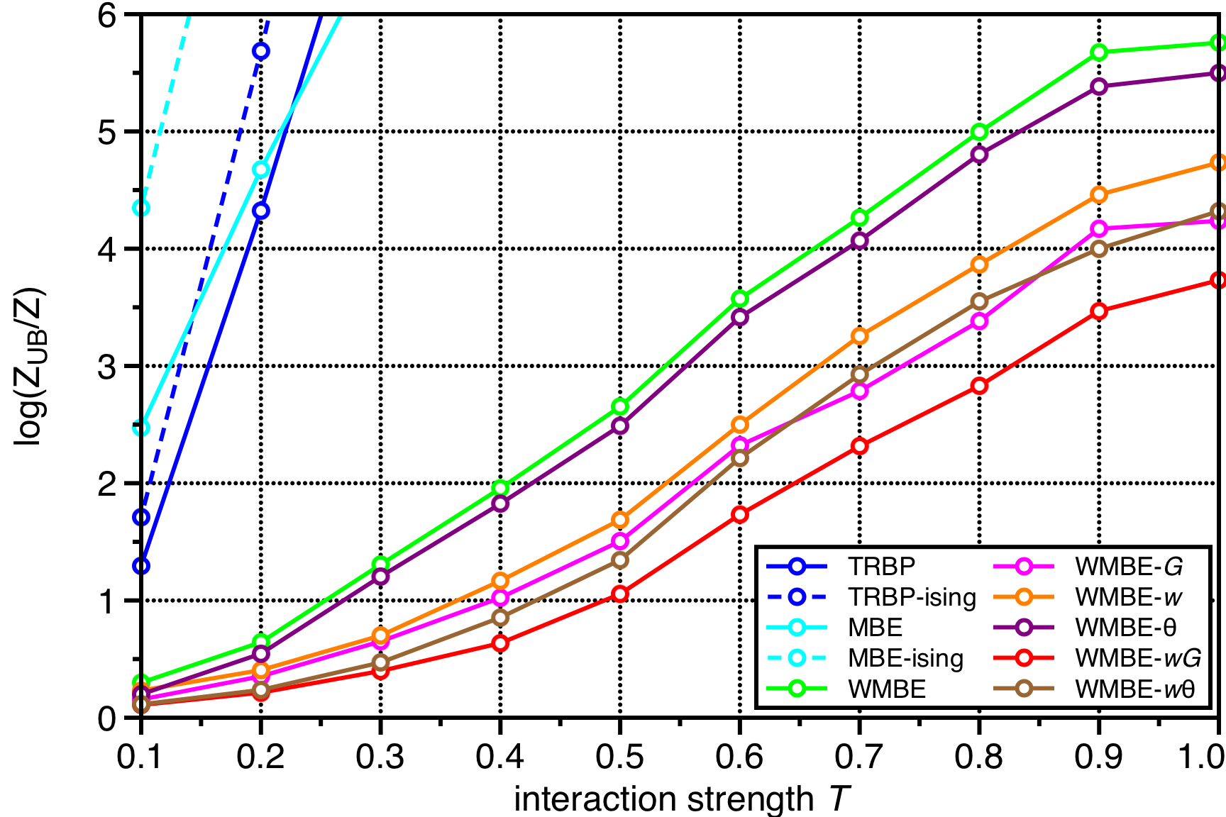
(b) Ising grid GMs, $ibound=6$

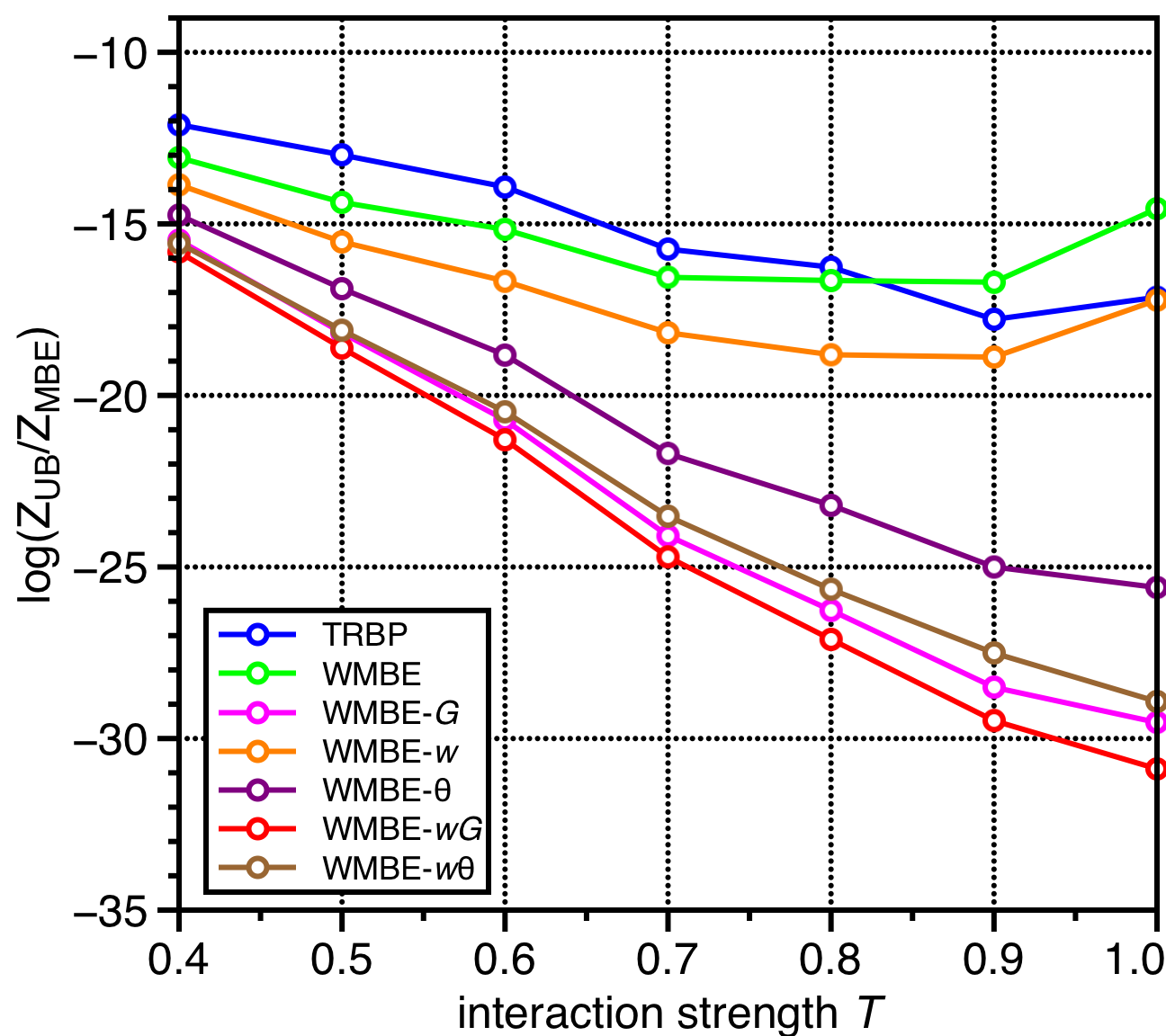
(c) $3$-regular GMs, $ibound=4$

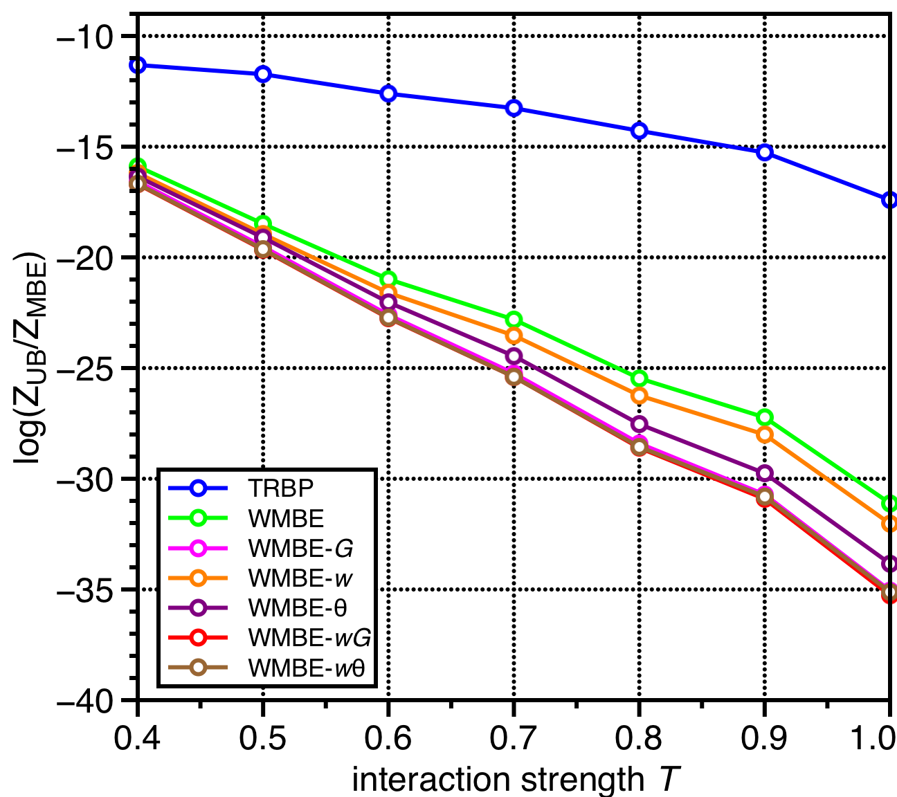
(d) $3$-regular GMs, $ibound=6$

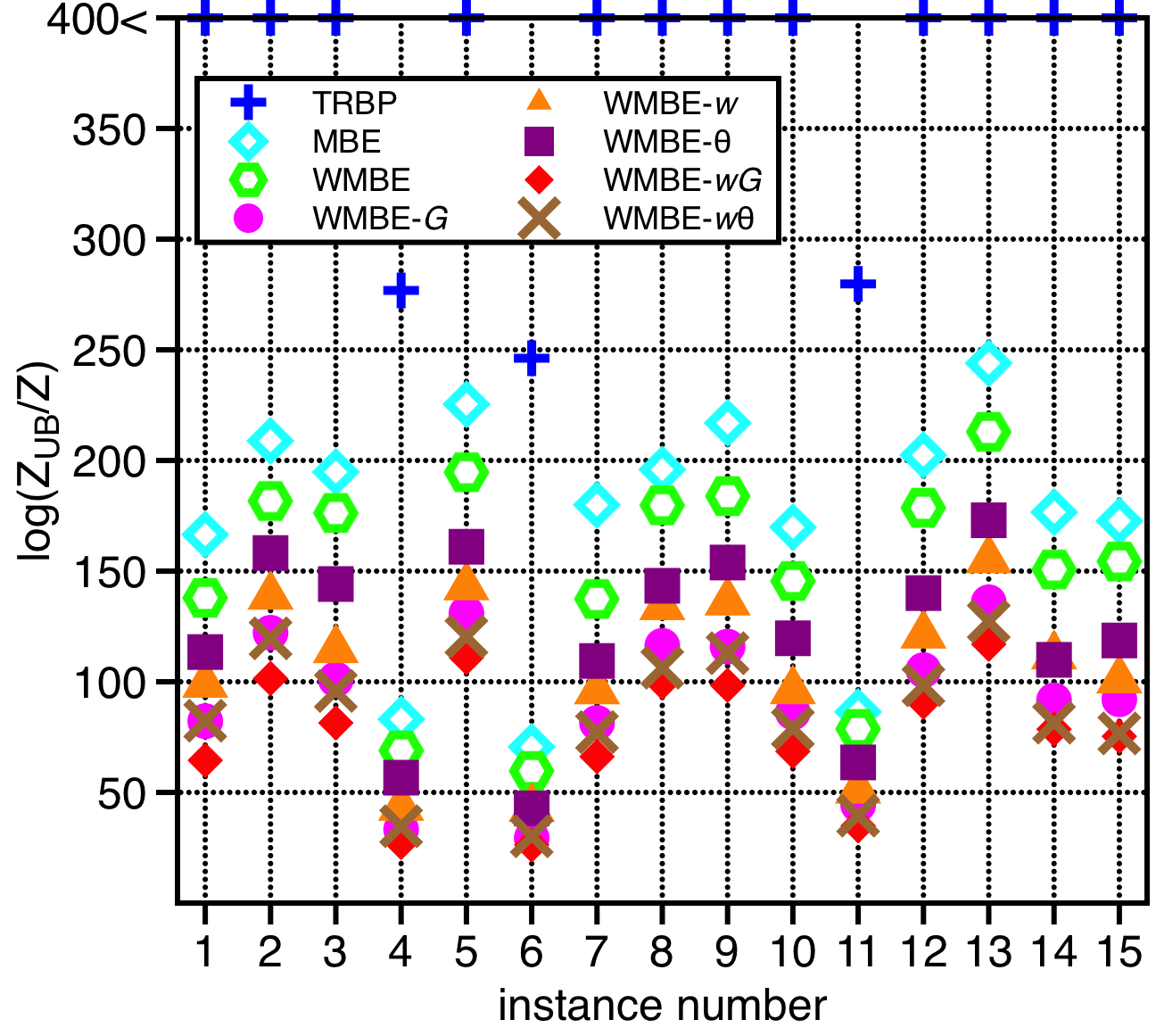
(e) Linkage dataset, $ibound=6$.

Figure 2: Performance comparisons in various families of GMs.

4.1 Setup

Experiments were conducted with three family of GMs: (i) Ising models on a $10\times 10$ grid graph (non-toroidal) with $180$ factors/$100$ variables; (ii) Forney-style GMs on the $3$-regular graph with $180$ factors/$270$ variables; and (iii) Linkage dataset from UAI 2014 Inference Competition [34].

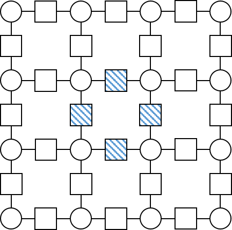
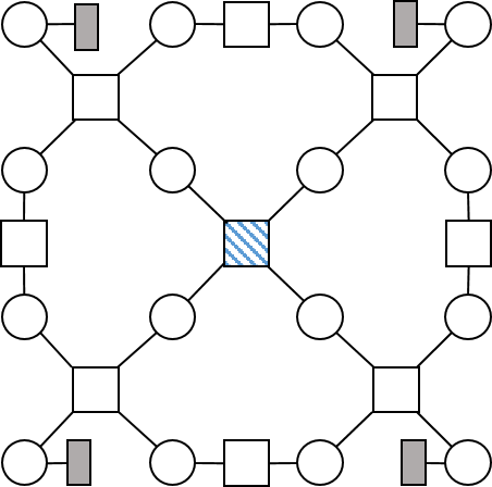
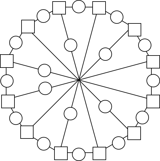
Figure 3: Illustration of Ising grid GM (left), its equivalent Forney-style GM (middle) and $3$-regular graph (right) of interest. Factors surrounding the selected lattice (blue, dashed) are contracted into a single factor, and then uniform single potentials (grey, filled) are added for variables of degree 1.

(i) Ising models. Ising models were defined with mixed interactions (spin glasses):

$$p(\mathbf{x})=\frac{1}{Z}\exp\big{(}\sum_{v\in X}\phi_{v}x_{v}+\sum_{(u,v)\in E}\phi_{uv}x_{u}x_{v}\big{)},$$

where $x_{u}\in\{-1,1\}$ and $\phi_{v}\sim\mathcal{N}(0,0.1)$, $\phi_{uv}\sim\mathcal{N}(0,T)$. Here, $T\geq 0$ is the ‘interaction strength’ parameter that controls the degree of interactions between variables. When $T=0$, variables are independent. As $T$ grows, the inference task is typically harder.

Note that this Ising model is not in Forney-style form, with variables adjacent to at most $4$ pairwise factors. Hence, to apply our gauge optimization framework, we generate an equivalent Forney-style GM using the transformation introduced in [30]: this maps any classical lattice model (allowing for magnetic fields/singleton potentials) into an equivalent Forney-style model. At a high level, the transformation chooses disjoint lattices to cover the whole graph, then contracts each lattice into a single factor. Levin and Nave [30] showed that one can always choose the lattice smartly so that each vertex is covered exactly twice, resulting in a Forney-style GM (see Figure 3 for details). Notably, this GM has relatively low induced width of $14$, thus the partition function can be computed exactly in reasonable time (though still computationally hard) by using BE.

(ii) 3-regular Forney-stlye GMs. We considered $3$-regular Forney-style GMs with log-factors drawn from normal distribution, i.e., $\log\mathnormal{f}_{\alpha}(\mathbf{x}_{\alpha})\sim\mathcal{N}(0,T)$. Again, $T\geq 0$ is the interaction strength parameter. In this case, we would like to choose graphs so that the induced width is high and the partition function is hard to compute. To this end, we aligned factors in a cycle, and assigned variables (edges) between adjacent factors in the cycle as well as those in the opposite side if it. See Figure 3 for its illustration. This choice gives high induced width, e.g., naïvely applying BE by eliminating variables between adjacent factors in clock-wise elimination order results in bucket size $2^{|V|/2+2}$.

(iii) UAI Linkage dataset. Finally, we consider a family of real-world models from the UAI 2014 Inference Competition, namely the Linkage (genetic linkage) dataset. Specifically, the family consists of GMs with average of $949.94$ variables with averaged maximum cardinality $\max_{i\in\mathcal{V}}|\mathcal{X}_{i}|=4.95$ and $727.35$ non-singleton hyper-edges with averaged maximum size $\max_{\alpha\in\mathcal{E}}|\alpha|=4.47$. Since GMs in Linkage dataset were not of Forney-style form, we constructed an equivalent Forney-style GM as in Figure 1.

Comparing approaches. We compared our gauged algorithm WMBE-G, i.e. optimizing the WMBE bound jointly with gauges and Hölder weights, to earlier methods considered in [16]: the unoptimized WMBE bound (‘WMBE’), its optimized versions with respect to Hölder weights $w$ and/or reparameterizations $\theta$ (‘WMBE-$w$’, ‘WMBE-$\theta$’ and ‘WMBE-$w\theta$’). Further, we also ran the following popular baselines for computing upper bounds on $Z$: standard mini-bucket elimination (‘MBE’) and tree re-weighted belief propagation (‘TRBP’) [12]. Finally, for fair comparisons in Ising grid GMs, we additionally compared to MBE and TRBP run on the original Ising grid GM (MBE-Ising and TRBP-Ising) in order to validate whether the forementioned GM transformation to a Forney-style model is ‘favored’ towards gauge optimization.

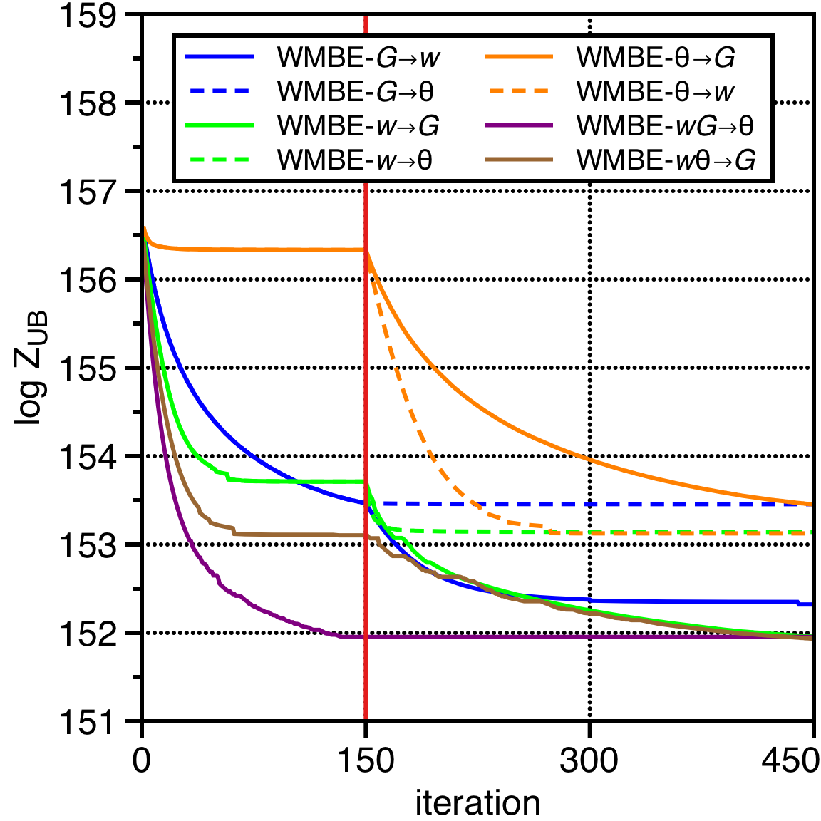
(a) Ising grid GMs, $ibound=4$

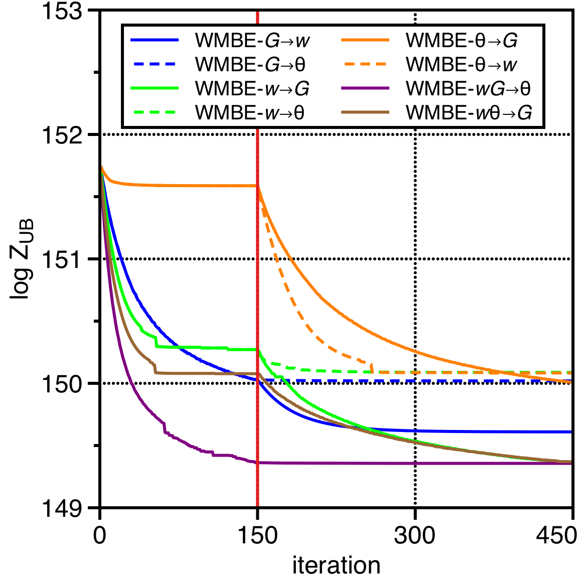
(b) Ising grid GMs, $ibound=6$

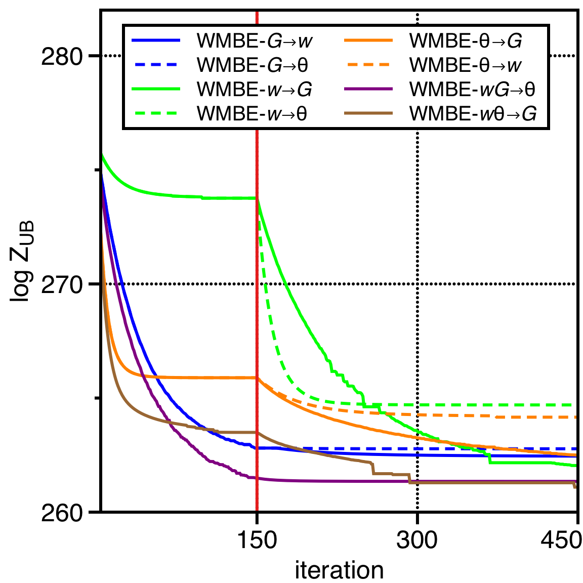
(c) $3$-regular GMs, $ibound=4$

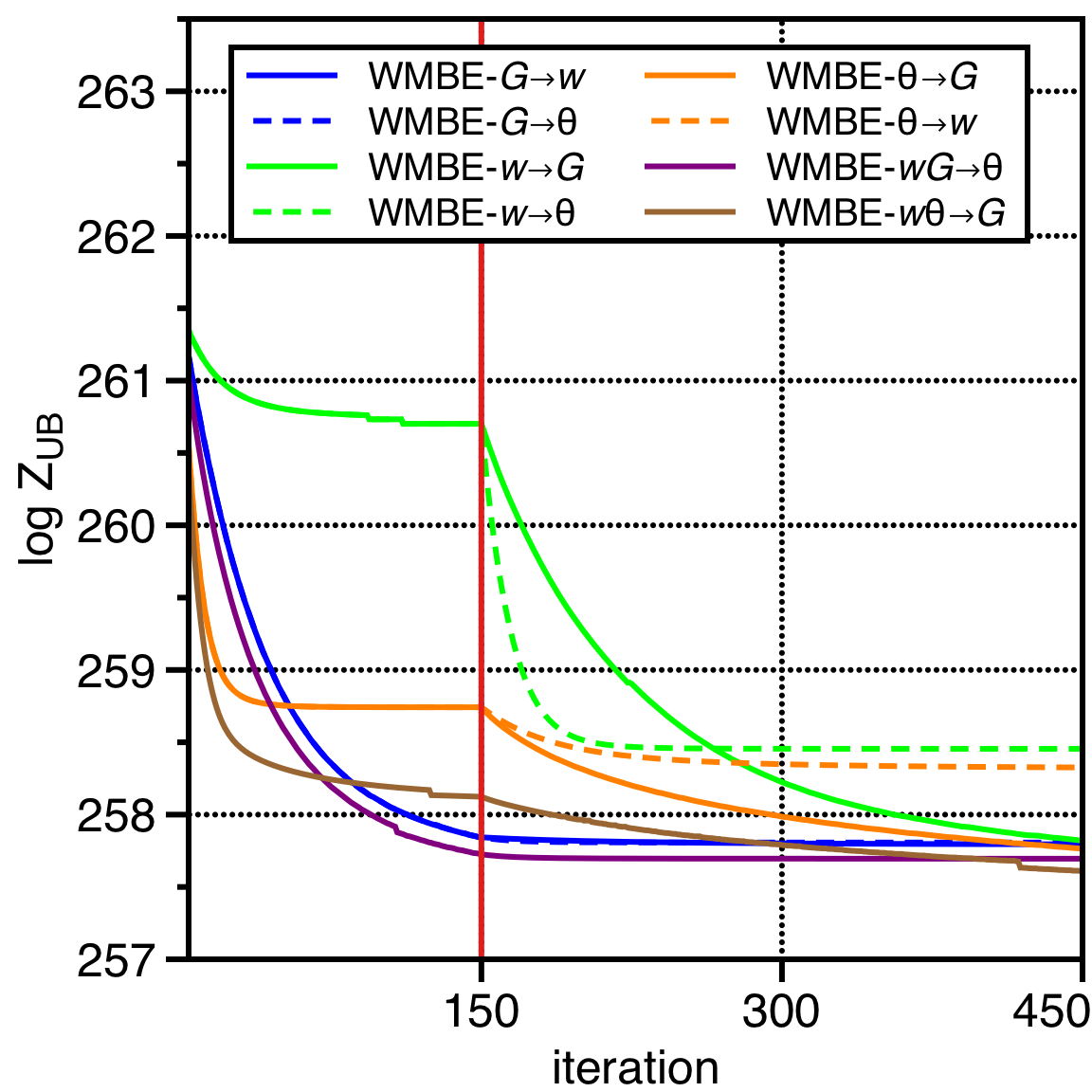
(d) $3$-regular GMs, $ibound=6$

Figure 4: Effectiveness of optimizing various parameter choices (all methods return an upper bound on $\log Z$).

Further details. Hölder weights $w$ and reparameterizations $\theta$ were updated using projected gradients and log-gradients respectively, as proposed in [16]. Step sizes for gradients were chosen as $0.01,0.1,0.1$ for optimizing each of gauge, Hölder weights, and reparameterizations, respectively. These were chosen empirically for ‘easy’ convergence in our experiments – there exists room for tuning or for more sophisticated gradient descent methods such as [35]. TRBP was run with damping until convergence. For Ising grid GMs, we measure the log-error (with base $e$) approximating the partition function $Z$, i.e., $\log\left({Z_{\text{UB}}}/{Z}\right)$ where $Z_{\text{UB}}$ is the upper bound of a respective algorithm. For $3$-regular GMs, it is impossible to measure (since $Z$ is impossible to compute), and instead we use the relative magnitude of bounds with respect to the mini-bucket upper bound $Z_{\text{MBE}}$, i.e., $\log\left({Z_{\text{UB}}}/{Z_{\text{MBE}}}\right)$. Since all tested algorithms provide guaranteed upper bounds on $Z$, a lower number indicates better performance. Further, in the UAI dataset, $2$ out of $17$ instances were omitted since it had factors with size larger than the algorithm’s $ibound$ of our choice. Finally, each point in the plots represents results averaged over $10$ independent runs.

4.2 Experimental Results

As shown in Figures 2(a)-(b), TRBP and MBE perform better on the transformed Forney-style GMs than on the original Ising models (this may be interesting to explore in future work), but not by nearly enough to achieve the performance of the other methods. For fair comparison, we should examine the ‘TRBP’ and ‘MBE’ plots rather than the ‘-Ising’ versions. We observe that WMBE-$wG$, which enjoys the most freedom in optimization of the WMBE bound, outperforms all other tested algorithms. In particular, the benefit of WMBE-$wG$ appears to increase with higher interaction strength. Comparing optimizations of just one class of parameters, i.e., WMBE-$G$, WMBE-$w$, WMBE-$\theta$, we observe that WMBE-$G$ performs at least as well as others. In particular, optimizing gauges is always better than optimizing over the subclass of reparameterizations, i.e., WMBE-$G$ and WMBE-$wG$ always outperform WMBE-$\theta$ and WMBE-$w\theta$, respectively. Further, WMBE-$G$ outperforms other approaches significantly for $3$-regular GMs and UAI dataset, where it outperforms even WMBE-$w\theta$ in $3$-regular GMs with $ibound=4$ and some instances of the UAI dataset.

Next, we consider experiments on specific instances of the Ising grid GM and $3$-regular GM with $T=1.0$ in order to measure the effectiveness of optimizing each parameter $G$, $w$, $\theta$ separately over iterations; see Figure 4. Specifically, we first optimize a chosen parameter with respect to WMBE related bounds (via gradient descent methods) for an initial $150$ iterations. Then, we change the parameter to optimize further (e.g., $G\rightarrow\theta$) for another $300$ iterations to observe the additional benefit from optimizing the second parameter. The running times per iteration for all parameters are comparable. We observe that $G$ methods perform very well, which is particularly impressive since we use a small step size for gauges. Overall, observed performance gains may be ranked as: gauges $>$ weights $>$ reparameterization for Ising grid GMs; and gauges $>$ reparameterization $>$ weights for 3-regular GMs. Gauge optimization is critical for the best performance in all experiments. As expected, $wG$ yields the best results. For 3-regular GMs, gauge optimization alone is almost optimal.

5 Conclusion

We developed a new gauge-variational approach to yield guaranteed bounds on the partition functions of GMs by jointly optimizing variational parameters and gauge transformations. Our approach has better scaling characteristics then other recent state-of-the-art methods, and should be of significant practical value.

Acknowledgements

AW acknowledges support from the David MacKay Newton research fellowship at Darwin College, The Alan Turing Institute under EPSRC grant EP/N510129/1 & TU/B/000074, and the Leverhulme Trust via the CFI. This work was partly supported by the ICT R&D program of MSIP/IITP [R-20161130-004520, Research on Adaptive Machine Learning Technology Development for Intelligent Autonomous Digital Companion]. The work of MC at LANL was carried out under the auspices of the National Nuclear Security Administration of the U.S. Department of Energy under Contract No. DE-AC52-06NA25396.

Supplement:

Gauged Mini-Bucket Elimination for Approximate Inference

Appendix A Example of Gauge Transformations

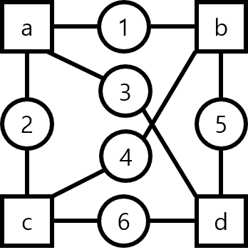
$$\mathnormal{f}_{a}(x_{1},x_{2},x_{3})=\left[\left[\begin{array}[]{cc}~{}2432&~{}~{}832\\ ~{}4672&~{}~{}640\end{array}\right]\left[\begin{array}[]{cc}~{}4864&~{}~{}384\\ ~{}5120&~{}4160\end{array}\right]\right]$$

$$\mathnormal{f}_{a}(x_{1},x_{2},x_{3};\mathbf{G}_{a})=\left[\left[\begin{array}[]{cc}~{}2837&~{}1559\\ ~{}3591&~{}2077\end{array}\right]\left[\begin{array}[]{cc}~{}3631&~{}2005\\ ~{}4261&~{}2077\end{array}\right]\right]$$

$$\mathnormal{f}_{b}(x_{1},x_{4},x_{5})=\left[\left[\begin{array}[]{cc}~{}1088&~{}~{}128\\ ~{}4928&~{}4608\end{array}\right]\left[\begin{array}[]{cc}~{}~{}448&~{}1664\\ ~{}3264&~{}1344\end{array}\right]\right]$$

$$\mathnormal{f}_{b}(x_{1},x_{4},x_{5};\mathbf{G}_{b})=\left[\left[\begin{array}[]{cc}~{}2142&~{}1434\\ ~{}4634&~{}4558\end{array}\right]\left[\begin{array}[]{cc}~{}~{}966&~{}1490\\ ~{}1490&~{}~{}758\end{array}\right]\right]$$

$$\mathnormal{f}_{c}(x_{2},x_{4},x_{6})=\left[\left[\begin{array}[]{cc}~{}1216&~{}5440\\ ~{}~{}768&~{}1856\end{array}\right]\left[\begin{array}[]{cc}~{}5568&~{}~{}896\\ ~{}~{}640&~{}~{}512\end{array}\right]\right]$$

$$\mathnormal{f}_{c}(x_{1},x_{4},x_{5};\mathbf{G}_{c})=\left[\left[\begin{array}[]{cc}~{}3960&~{}8808\\ \text{-}1608&\text{-}2520\end{array}\right]\left[\begin{array}[]{cc}~{}\text{-}328&\text{-}3288\\ ~{}6520&~{}8296\end{array}\right]\right]$$

$$\mathnormal{f}_{d}(x_{3},x_{5},x_{6})=\left[\left[\begin{array}[]{cc}~{}5632&~{}5632\\ ~{}6080&~{}6208\end{array}\right]\left[\begin{array}[]{cc}~{}5568&~{}~{}896\\ ~{}~{}640&~{}~{}512\end{array}\right]\right]$$

$$\mathnormal{f}_{d}(x_{3},x_{5},x_{6};\mathbf{G}_{d})=\left[\left[\begin{array}[]{cc}~{}2408&~{}9160\\ 10760&~{}9192\end{array}\right]\left[\begin{array}[]{cc}14536&\text{-}6232\\ \text{-}7448&\text{-}1208\end{array}\right]\right]$$

$$G_{1a},G_{2a},G_{3a},G_{4b},G_{5b},G_{6c}=\left[\begin{array}[]{cc}0.75&0.25\\ 0.25&0.75\end{array}\right]$$

$$G_{1b},G_{2c},G_{3d},G_{4c},G_{5d},G_{6d}=\left[\begin{array}[]{cc}1.5&\text{-}0.5\\ \text{-}0.5&1.5\end{array}\right]$$

Figure 5: Example of gauge transformations on the complete graph (with respect to factors) of size $4$. Arrays follow row-column major indexing, e.g., $\mathnormal{f}_{a}(1,1,2)=4864$ and $\mathnormal{f}_{a}(1,2,1)=832$.

Appendix B Proof of Theorem 1

We prove reparameterization with respect to $\boldsymbol{\theta}=\{\theta_{v\alpha}(x_{v})=0,~{}\forall(v,\alpha)\in E,x_{v}\}$ is optimal at GM with symmetric factors in the following optimization:

$$\operatornamewithlimits{\mbox{minimize}}_{\boldsymbol{\theta}}\quad \operatorname*{\mathchoice{\ooalign{\phantom{$\displaystyle\sum$}\cr\raisebox{1.2pt}{$\mkern 22.0mu\scalebox{0.7}{$\circ$}$}\cr\raisebox{-0.7pt}{$\mkern 22.0mu\scalebox{0.7}{$\circ$}$}\cr$\displaystyle\sum$}}{\ooalign{$\textstyle\sum$\cr\raisebox{1.9pt}{$\mkern 16.0mu\scalebox{0.4}{$\circ$}$}\cr\raisebox{-0.3pt}{$\mkern 16.0mu\scalebox{0.4}{$\circ$}$}\cr}}{\ooalign{\raisebox{0.0pt}{\scalebox{0.6}{$\scriptstyle\sum$}}\cr\raisebox{1.6pt}{$\mkern 7.5mu\scalebox{0.2}{$\circ$}$}\cr\raisebox{-0.2pt}{$\mkern 7.5mu\scalebox{0.2}{$\circ$}$}\cr}}{\ooalign{\raisebox{0.2pt}{\scalebox{0.6}{$\scriptstyle\sum$}}\cr\raisebox{2.2pt}{$\mkern 7.5mu\scalebox{0.2}{$\circ$}$}\cr\raisebox{0.4pt}{$\mkern 7.5mu\scalebox{0.2}{$\circ$}$}\cr}}}^{\bar{w}_{\bar{n}}}_{\bar{x}_{\bar{1}}}\cdots\operatorname*{\mathchoice{\ooalign{\phantom{$\displaystyle\sum$}\cr\raisebox{1.2pt}{$\mkern 22.0mu\scalebox{0.7}{$\circ$}$}\cr\raisebox{-0.7pt}{$\mkern 22.0mu\scalebox{0.7}{$\circ$}$}\cr$\displaystyle\sum$}}{\ooalign{$\textstyle\sum$\cr\raisebox{1.9pt}{$\mkern 16.0mu\scalebox{0.4}{$\circ$}$}\cr\raisebox{-0.3pt}{$\mkern 16.0mu\scalebox{0.4}{$\circ$}$}\cr}}{\ooalign{\raisebox{0.0pt}{\scalebox{0.6}{$\scriptstyle\sum$}}\cr\raisebox{1.6pt}{$\mkern 7.5mu\scalebox{0.2}{$\circ$}$}\cr\raisebox{-0.2pt}{$\mkern 7.5mu\scalebox{0.2}{$\circ$}$}\cr}}{\ooalign{\raisebox{0.2pt}{\scalebox{0.6}{$\scriptstyle\sum$}}\cr\raisebox{2.2pt}{$\mkern 7.5mu\scalebox{0.2}{$\circ$}$}\cr\raisebox{0.4pt}{$\mkern 7.5mu\scalebox{0.2}{$\circ$}$}\cr}}}^{\bar{w}_{1}}_{\bar{x}_{1}}\prod_{\alpha\in F}\mathnormal{f}_{\alpha}(\bar{\mathbf{x}}_{\alpha};\boldsymbol{\theta}_{\alpha}),$$

subject to $$\prod_{\alpha\in N(v)}\exp(\theta_{v\alpha}(x_{v}))=1\quad\forall~{}v\in X,x_{v}.$$

The optimization is convex, and assuming $\theta_{v\beta}+\theta_{v\alpha}=0$ from the constraint, $\partial\log Z_{\text{WMBE}}/\partial\theta_{v\alpha}=0$ implies optimality of the solution. To this end, the derivative is expressed as:

$$\frac{\partial\log Z_{\text{WMBE}}}{\partial\bar{\theta}_{\alpha}(\mathbf{x}_{v\alpha})}=\sum_{\mathbf{x}_{\alpha\backslash v}}q(\bar{\mathbf{x}}_{\alpha})-\sum_{\mathbf{\bar{x}}_{\beta\backslash v}}q(\bar{\mathbf{x}}_{\beta}).$$

When factors are symmetric, it immediately follows that

$$\sum_{\mathbf{x}_{\alpha\backslash v}}q(\bar{\mathbf{x}}_{\alpha})=\sum_{\mathbf{\bar{x}}_{\beta\backslash v}}q(\bar{\mathbf{x}}_{\beta})=0.5,$$

since $q$ is expressed via weighted absolute sum and normalization operation of factors, which both preserve symmetry. Hence marginals are also symmetric, implying uniform distribution. Hence the optimality condition is satisfied.

References

- [1] Robert Gallager. Low-density parity-check codes. IRE Transactions on information theory, 8(1):21–28, 1962.
- [2] Frank R. Kschischang and Brendan J. Frey. Iterative decoding of compound codes by probability propagation in graphical models. IEEE Journal on Selected Areas in Communications, 16(2):219–230, 1998.
- [3] Hans A. Bethe. Statistical theory of superlattices. Proceedings of Royal Society of London A, 150:552, 1935.
- [4] Rudolf E. Peierls. Ising’s model of ferromagnetism. Proceedings of Cambridge Philosophical Society, 32:477–481, 1936.
- [5] Marc Mézard, Georgio Parisi, and M. A. Virasoro. Spin Glass Theory and Beyond. Singapore: World Scientific, 1987.
- [6] Giorgio Parisi. Statistical field theory, 1988.
- [7] Marc Mezard and Andrea Montanari. Information, Physics, and Computation. Oxford University Press, Inc., New York, NY, USA, 2009.
- [8] Judea Pearl. Probabilistic reasoning in intelligent systems: networks of plausible inference. Morgan Kaufmann, 2014.
- [9] Michael I. Jordan. Learning in graphical models, volume 89. Springer Science & Business Media, 1998.
- [10] William T. Freeman, Egon C. Pasztor, and Owen T. Carmichael. Learning low-level vision. International journal of computer vision, 40(1):25–47, 2000.
- [11] Mark Jerrum and Alistair Sinclair. Polynomial-time approximation algorithms for the Ising model. SIAM Journal on computing, 22(5):1087–1116, 1993.
- [12] Martin J. Wainwright, Tommi S. Jaakkola, and Alan S. Willsky. A new class of upper bounds on the log partition function. IEEE Transactions on Information Theory, 51(7):2313–2335, 2005.
- [13] Judea Pearl. Reverend Bayes on inference engines: A distributed hierarchical approach. Cognitive Systems Laboratory, School of Engineering and Applied Science, University of California, Los Angeles, 1982.
- [14] Qiang Liu and Alexander Ihler. Negative tree reweighted belief propagation. In Proceedings of the Twenty-Sixth Conference on Uncertainty in Artificial Intelligence, pages 332–339. AUAI Press, 2010.
- [15] Stefano Ermon, Ashish Sabharwal, Bart Selman, and Carla P. Gomes. Density propagation and improved bounds on the partition function. In Advances in Neural Information Processing Systems, pages 2762–2770, 2012.
- [16] Qiang Liu and Alexander T. Ihler. Bounding the partition function using Hölder’s inequality. In Proceedings of the 28th International Conference on Machine Learning (ICML-11), pages 849–856, 2011.
- [17] Alexander Novikov, Anton Rodomanov, Anton Osokin, and Dmitry Vetrov. Putting MRFs on a tensor train. In International Conference on Machine Learning, pages 811–819, 2014.
- [18] Martin J. Wainwright, Tommy S. Jaakkola, and Alan S. Willsky. Tree-based reparametrization framework for approximate estimation on graphs with cycles. Information Theory, IEEE Transactions on, 49(5):1120–1146, 2003.
- [19] Michael Chertkov and Vladimir Chernyak. Loop calculus in statistical physics and information science. Physical Review E, 73:065102(R), 2006.
- [20] Michael Chertkov and Vladimir Chernyak. Loop series for discrete statistical models on graphs. Journal of Statistical Mechanics, page P06009, 2006.
- [21] Leslie G. Valiant. Holographic algorithms. SIAM Journal on Computing, 37(5):1565–1594, 2008.
- [22] Ali Al-Bashabsheh and Yongyi Mao. Normal factor graphs and holographic transformations. IEEE Transactions on Information Theory, 57(2):752–763, 2011.
- [23] Martin J. Wainwright and Michael I. Jordan. Graphical models, exponential families, and variational inference. Foundations and Trends in Machine Learning, 1(1):1–305, 2008.
- [24] G. David Forney Jr and Pascal O. Vontobel. Partition functions of normal factor graphs. arXiv preprint arXiv:1102.0316, 2011.
- [25] Michael Chertkov. Lecture notes on “statistical inference in structured graphical models: Gauge transformations, belief propagation & beyond”, https://sites.google.com/site/mchertkov/courses, 2016.
- [26] Sung-Soo Ahn, Michael Chertkov, and Jinwoo Shin. Gauging variational inference. In Advances in Neural Information Processing Systems 30, pages 2881–2890. Curran Associates, Inc., 2017.
- [27] Andreas Wächter and Lorenz T Biegler. On the implementation of an interior-point filter line-search algorithm for large-scale nonlinear programming. Mathematical programming, 106(1):25–57, 2006.
- [28] Rina Dechter and Irina Rish. Mini-buckets: A general scheme for bounded inference. Journal of the ACM (JACM), 50(2):107–153, 2003.
- [29] G. David Forney. Codes on graphs: Normal realizations. IEEE Transactions on Information Theory, 47(2):520–548, 2001.
- [30] Michael Levin and Cody P. Nave. Tensor renormalization group approach to two-dimensional classical lattice models. Physical review letters, 99(12):120601, 2007.
- [31] Rina Dechter. Bucket elimination: A unifying framework for reasoning. Artificial Intelligence, 113(1):41–85, 1999.
- [32] Daphne Koller and Nir Friedman. Probabilistic graphical models: principles and techniques. MIT press, 2009.
- [33] G.H. Hardy, J.E. Littlewood, and G. Pólya. Inequalities, 1934.
- [34] Vibhav Gogate. UAI 2014 Inference Competition. http://www.hlt.utdallas.edu/~vgogate/uai14-competition/index.html, 2014.
- [35] Yurii Nesterov. A method of solving a convex programming problem with convergence rate o(1/k2). Soviet Mathematics Doklady, 27(2):372–376, 1983.