Nucleon Axial and Electromagnetic Form Factors

Abstract

We present results for the isovector axial, induced pseudoscalar, electric, and magnetic form factors of the nucleon. The calculations were done using $2+1+1$-flavor HISQ ensembles generated by the MILC collaboration with lattice spacings $a\approx$ 0.12, 0.09, 0.06 $\mathrm{fm}$ and pion masses $M_{\pi}\approx$ 310, 220, 130 $\mathrm{MeV}$. Excited-states contamination is controlled by using four-state fits to two-point correlators and by comparing two- versus three-states in three-point correlators. The $Q^{2}$ behavior is analyzed using the model independent z-expansion and the dipole ansatz. Final results for the charge radii and magnetic moment are obtained using a simultaneous fit in $M_{\pi}$, lattice spacing $a$ and finite volume.

1 Introduction

To extract the form factors from the three-point correlators, we consider the spectral decomposition including contributions from three states, the ground state $\lvert 0\rangle$ and two excited states $\lvert 1\rangle,\lvert 2\rangle$:

$$C_{\Gamma}^{(3\text{pt})}(t;\tau;\bm{p}^{\prime},\bm{p}) =\lvert\mathcal{A}_{0}^{\prime}\rvert\lvert\mathcal{A}_{0}\rvert\langle 0^{\prime}\lvert\mathcal{O}_{\Gamma}\rvert 0\rangle e^{-E_{0}t-M_{0}(\tau-t)}$$

$$\;+\lvert\mathcal{A}_{0}^{\prime}\rvert\lvert\mathcal{A}_{1}\rvert\langle 0^{\prime}\lvert\mathcal{O}_{\Gamma}\rvert 1\rangle e^{-E_{0}t-M_{1}(\tau-t)}+\lvert\mathcal{A}_{1}^{\prime}\rvert\lvert\mathcal{A}_{0}\rvert\langle 1^{\prime}\lvert\mathcal{O}_{\Gamma}\rvert 0\rangle e^{-E_{1}t-M_{0}(\tau-t)}$$

$$\;+\lvert\mathcal{A}_{1}^{\prime}\rvert\lvert\mathcal{A}_{1}\rvert\langle 1^{\prime}\lvert\mathcal{O}_{\Gamma}\rvert 1\rangle e^{-E_{1}t-M_{1}(\tau-t)}$$

$$\;+\lvert\mathcal{A}_{0}^{\prime}\rvert\lvert\mathcal{A}_{2}\rvert\langle 0^{\prime}\lvert\mathcal{O}_{\Gamma}\rvert 2\rangle e^{-E_{0}t-M_{2}(\tau-t)}+\lvert\mathcal{A}_{2}^{\prime}\rvert\lvert\mathcal{A}_{0}\rvert\langle 2^{\prime}\lvert\mathcal{O}_{\Gamma}\rvert 0\rangle e^{-E_{2}t-M_{0}(\tau-t)}$$

$$\;+\lvert\mathcal{A}_{1}^{\prime}\rvert\lvert\mathcal{A}_{2}\rvert\langle 1^{\prime}\lvert\mathcal{O}_{\Gamma}\rvert 2\rangle e^{-E_{1}t-M_{2}(\tau-t)}+\lvert\mathcal{A}_{2}^{\prime}\rvert\lvert\mathcal{A}_{1}\rvert\langle 2^{\prime}\lvert\mathcal{O}_{\Gamma}\rvert 1\rangle e^{-E_{2}t-M_{1}(\tau-t)}$$

$$\;+\lvert\mathcal{A}_{2}^{\prime}\rvert\lvert\mathcal{A}_{2}\rvert\langle 2^{\prime}\lvert\mathcal{O}_{\Gamma}\rvert 2\rangle e^{-E_{2}t-M_{2}(\tau-t)}\,.$$ (1)

In our lattice calculation, $\bm{p}=\bm{0}$ and the three states have mass $M_{i}$. The primed states $\lvert j^{\prime}\rangle$ have momentum $\bm{p}^{\prime}$ and energy $E_{j}$. The desired matrix element is $\langle 0^{\prime}\lvert\mathcal{O}_{\Gamma}\rvert 0\rangle$, which can be decomposed into nucleon form factors, associated with all possible Lorentz covariant structures for a given current insertion $O_{\Gamma}$. To estimate convergence of the truncated spectral decomposition, we compare results of 2-state fits (neglecting contributions of the second excited state) with a $3^{\ast}$-state fit in which the poorly determined matrix element $\langle 2^{\prime}\lvert\mathcal{O}_{\Gamma}\rvert 2\rangle$ is set to zero. Within the single elimination jackknife process, we use results of 4-state fits to the two-point correlator to obtain the energy $E_{i}$, mass $M_{i}$ and amplitudes $\mathcal{A}_{i}^{(\prime)}$ that are inputs in the fits to the three-point correlators using Eq. (1).

Table 1: Fit parameters. The $2^{nd}$ column gives the fit ranges used for nucleon two-point correlators. The $3^{rd}$ column gives the values of source-sink separations $\tau$ simulated and used in the fits, and the $4^{th}$ column gives the number of timeslices, $t_{\text{skip}}$, adjacent to the source and the sink, skipped in the fits to three-point correlators to control excited-state contamination. The $5^{th}$ column gives the value of $\bar{t}_{0}$ chosen in the $z-$expansion fit at which $z(Q^{2}=\bar{t}_{0})=0$. The fit ranges for ensembles a09m310 and a09m220 are different from those in Rajan:2017lxk , since these ensembles have been updated with higher statistics AMA bias corrected data, and include data with $\tau=16$ and momentum insertion up to $n^{2}=10$. The calculation of the $Q^{2}\neq 0$ data for the a09m130 ensemble has been analyized using only the low precision data.

ensemble	$[t_{\text{min}},t_{\text{max}}]$	$\{\tau\}$	$t_{\text{skip}}$	$\bar{t}_{0}$	$L^{3}\times T$	$M_{\pi}^{\rm val}L$	$N_{\text{conf}}$	$N_{\rm meas}^{\rm HP}$	$N_{\rm meas}^{\rm{LP}}$
a12m310	$[2,15]$	{8,10,12}	2	0.40	$24^{3}\times 64$	4.55	1013	8104	64,832
a12m220L	$[2,15]$	{8,10,12,14}	2	0.20	$40^{3}\times 64$	5.49	1010	8080	68,680
a09m310	$[2,18]$	{10,12,14,16}	3	0.50	$32^{3}\times 96$	4.51	2264	9056	114,896
a09m220	$[3,20]$	{10,12,14,16}	3	0.40	$48^{3}\times 96$	4.79	964	3856	123,392
a09m130	$[4,20]$	{10,12,14}	3	0.12	$64^{3}\times 96$	3.90	883	7064	56,512
a06m310	$[7,30]$	{16,20,22,24}	7	0.40	$48^{3}\times 144$	4.52	1000	8000	64,000
a06m220	$[7,30]$	{16,20,22,24}	7	0.20	$64^{3}\times 144$	4.41	650	2600	41,600
a06m135	$[6,30]$	{16,18,20,22}	6	0.12	$96^{3}\times 192$	3.74	322	1288	20,608

2 Axial Form Factor

Nucleon matrix elements with the insertion of the isovector axial vector current can be decomposed into the axial form factor $G_{A}$ and the induced pseudoscalar form factor $\tilde{G}_{P}$:

$$\left\langle N(\bm{p}_{f})|A_{\mu}(\bm{q})|N(\bm{p}_{i})\right\rangle =\;{\overline{u}}_{N}(\bm{p}_{f})\left(G_{A}(Q^{2})\gamma_{\mu}+q_{\mu}\frac{\tilde{G}_{P}(Q^{2})}{2M_{N}}\right)\gamma_{5}u_{N}(\bm{p}_{i}),$$ (2)

where $Q^{2}\equiv\bm{p}^{2}-(E-m)^{2}=-q^{2}$ and $q=p_{f}-p_{i}$. Note that $\bm{p}_{i}=0$ in our lattice calculation. Results for the axial form factor $G_{A}(Q^{2})$, normalized by the corresponding $g_{A}\equiv G_{A}(0)$ for each of the 8 ensembles, are shown in Fig. 1. A notable change on going from 2-state fits presented in Ref. Rajan:2017lxk to $3^{\ast}$-state fits is the much better agreement in the data from the two physical mass ensembles and in the final estimates given in Table 5. For each ensemble, the axial charge radius $\langle r_{A}^{2}\rangle$ is obtained from the analytic derivative of the dipole and the $z$-expansion fits evaluated at $Q^{2}=0$ as explained in Ref. Rajan:2017lxk .

The chiral, continuum, and finite volume (FV) extrapolation to $M_{\pi}\to 135\;\mathrm{MeV}$, $a\to 0$ and $M_{\pi}L\to\infty$ is performed using only the leading order correction terms:

$$\langle r_{A}^{2}\rangle(a,M_{\pi},L)=c_{1}^{A}+c_{2}^{A}a+c_{3}^{A}M_{\pi}^{2}+c_{4}^{A}M_{\pi}^{2}\exp(-M_{\pi}L)$$ (3)

In all the results presented in this talk, the FV term is small and $c^{A,S,T}_{4}$ are not well determined. Nevertheless, results with and without the FV term are consistent as shown in Tables 2,  3 and 4 where we give results with and without the FV term, compare the 2- and $3^{\ast}$-state fits used to control excited-state contamination, and the $z-$expansion versus the dipole fits for the $Q^{2}$ behavior. A detailed description of our analysis methodology is presented in Ref. Rajan:2017lxk for the axial form factor.

For our final estimates summarized in Table 5, we separately quote the weighted average of the two $z$-expansion fits and the dipole results given in Table 2 including the finite volume term. We also quote $\mathcal{M}_{A}^{2}\equiv 12/r_{A}^{2}$ for both the dipole and the $z-$expansion data.

These results are consistent with our previously reported values in Ref. Rajan:2017lxk . Our new central values from the $3^{\ast}$-state fit agree with the MiniBooNE results $\mathcal{M}_{A}=1.35(17)\;\mathrm{GeV}$ AguilarArevalo:2010zc , but differ by about $1\,\sigma$ from the 2-state fit results and by about $2.5\,\sigma$ from the phenomenological estimate $r_{A}=0.666(17)\,\mathrm{fm}$ Bernard:1998gv obtained using the neutrino scattering data. A recent reanalysis of the deuterium data based on the $z$-expansion assesses an order of magnitude larger error, $r_{A}=0.68(16)\,\mathrm{fm}$ Meyer:2016oeg , in which case the disagreement with our $3^{\ast}$-state result reduces to about $1\sigma$.

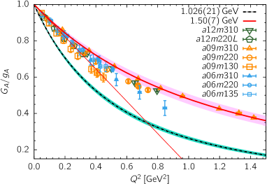
(a) 2-state

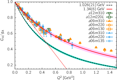
(b) $3^{\ast}$-state

Figure 1: Axial form factor data from the 2- and $3^{\ast}$-state fits to the three-point functions. The thick red line within the pink band shows the dipole result given in Table 5, and the thin straight red line is the slope, $-r_{A}^{2}/6$, at zero momentum transfer. Both the $z-$expansion and the dipole estimates differ from the dipole fit with the phenominological estimate, $\mathcal{M}_{A}=1.026(21)\,\mathrm{GeV}$ given in Ref. Bernard:2001rs , that represents the world average from the neutrino scattering data. Note also the change in the slope, $-r_{A}^{2}/6$, between the 2- and $3^{\ast}$-state fits. This trend is the same for the $z$-expansion estimates.

Table 2: Estimates for the mean square axial charge radius $\langle r_{A}^{2}\rangle$. The first column lists the terms kept in the continuum chiral extrapolation fit using Eq. (3). Data from each of the eight ensembles described in Table 1 are analyzed using both the $2$-state and $3^{\ast}$-state truncation of the spectral decomposition of the three-point correlator given in Eq. (1), followed by dipole and $z$-expansion (including sumrule constraints) fits described in Ref. Rajan:2017lxk .

	$2$-state			$3^{\ast}$-state
	dipole	$z^{2+4}$	$z^{3+4}$	dipole	$z^{2+4}$	$z^{3+4}$
$a$, $M_{\pi}^{2}$, FV	0.208(19)	0.180(37)	0.223(60)	0.260(25)	0.245(52)	0.272(89)
$a$, $M_{\pi}^{2}$	0.214(15)	0.166(29)	0.172(48)	0.248(20)	0.219(46)	0.219(79)

3 Pseudoscalar Form Factor

Data for the normalized induced pseudoscalar form factor, $(m_{\mu}/2M_{N})\tilde{G}_{P}/g_{A}$ with $m_{\mu}$ the muon mass, are summarized in Fig. 2. They show essentially no dependence on $M_{\pi}$ or $a$ or $M_{\pi}L$. In Ref. Rajan:2017lxk , we highlighted a problem in the extraction of $\tilde{G}_{P}$: the three form factors $G_{A}$, $\tilde{G}_{P}$, and the pseudoscalar form factor $G_{P}$ do not satisfy the axial Ward identity. As a result, the pion-pole dominance ansatz used to extrapolate the lattice data for $\tilde{G}_{P}$ at fixed $Q^{2}$ in $M_{\pi}^{2}$, to obtain say $g_{P}^{\ast}\equiv m_{\mu}/2M_{N}\times\tilde{G}_{P}(Q^{2}=0.88m_{\mu}^{2})$, was shown to also fail. In fact, our results for $g_{P}^{\ast}$ from the two physical pion mass ensembles are about half the muon capture experiment result Rajan:2017lxk . A similar underestimate also occurs for the pion-nucleon coupling $g_{\pi{\rm NN}}$. In Ref. Rajan:2017lxk , we further show that $\mathcal{O}(a)$ improvement of the axial current operator does not significantly reduce the problem. Updated data presented here in Fig. 2, show only a small increase in the values of the form factor at low $Q^{2}$ on going from the 2-state to the $3^{\ast}$-state analysis. Thus, the violation of PCAC in the extraction of $\tilde{G}_{P}$ remains an unresolved problem.

(a) 2-state

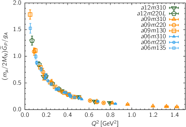
(b) $3^{\ast}$-state

Figure 2: Data for the normalized pseudoscalar form factor $(m_{\mu}/2M_{N})\tilde{G}_{P}/g_{A}$ for the 8 ensembles.

4 The Electric Form Factor

Nucleon matrix elements with vector current insertion can be decomposed into the Dirac and Pauli form factors $F_{1}$ and $F_{2}$ as:

$$\left\langle N(\bm{p}_{f})|V_{\mu}(\bm{q})|N(\bm{p}_{i})\right\rangle =\;{\overline{u}}_{N}(\bm{p}_{f})\left(F_{1}(Q^{2})\gamma_{\mu}+\sigma_{\mu\nu}\frac{F_{2}(Q^{2})}{2M_{N}}\right)\gamma_{5}u_{N}(\bm{p}_{i}).$$ (4)

Here, we present results for the related Sachs, the electric and the magnetic, form factors $G_{E}$ and $G_{M}$:

$$G_{E}(Q^{2}) =F_{1}(Q^{2})-\frac{Q^{2}}{4M_{N}^{2}}F_{2}(Q^{2})\,,$$ (5)

$$G_{M}(Q^{2}) =F_{1}(Q^{2})+F_{2}(Q^{2})\,.$$ (6)

The data for $G_{E}(Q^{2})$ is summarized in Fig. 3, and we find that the $3^{\ast}$-state fits are closer to the phenomenological curve compared to the $2$-state fits. The charge radii $\langle r_{E}^{2}\rangle$ and $\langle r_{M}^{2}\rangle$ on each ensemble are then extracted following the same procedure as for $\langle r_{A}^{2}\rangle$. From these, the continuum chiral extrapolation for the electric charge radius is performed using the following ansatz:

$$\langle r_{E}^{2}\rangle(a,M_{\pi},L)=c_{1}^{E}+c_{2}^{E}a+c_{3}^{E}\ln(M_{\pi}^{2}/\lambda^{2})+c_{4}^{E}\ln(M_{\pi}^{2}/\lambda^{2})\exp(-M_{\pi}L)\,,$$ (7)

where the mass scale $\lambda$ is chosen to be $M_{\rho}=775\,\mathrm{MeV}$ and the form of the chiral and FV corrections are taken from Refs. Bernard:1998gv ; Gockeler:2003ay : Using Eq. (7), the results for the different fit ansatz are summarized in Table 3. For the final estimates given in Table 5, we take the weighted average of the two $z$-expansion fits given in Table 3. The $z$-expansion and the dipole fit results with the $3^{\ast}$-state analysis overlap. All four estimates are smaller than the CODATA-2014 world average, $r_{E}=0.875(6)\,\mathrm{fm}$ Mohr:2015ccw , from the electron experiments and the more accurate value derived from the Lamb shift in muonic hydrogen, $r_{E}=0.8409(4)\,\mathrm{fm}$ Antognini:2015moa ; the $z$-expansion result with $3^{\ast}$-state analysis is consistent with the experiments because of the error estimate is larger.

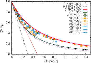
(a) 2-state

(b) $3^{\ast}$-state

Figure 3: The 8 ensemble data for the normalized electric form factor ${G}_{E}/g_{V}$. The overlaid red band shows our dipole result given in Table 5. The black dashed line shows the phenomenological value $\mathcal{M}_{E}=0.780(5)$ in both panels. The corresponding straight lines give their slopes, $-r_{E}^{2}/6$, at $Q^{2}=0$. Experimental data paramterized by the Kelly curve is shown by the purple dotted line.

Table 3: Mean square electric charge radius $\langle r_{E}^{2}\rangle$. The first column shows the terms included in the chiral continuum extrapolation defined in Eq. (3). The rest is the same as in Table 2.

	$2$-state			$3^{\ast}$-state
	dipole	$z^{2+4}$	$z^{3+4}$	dipole	$z^{2+4}$	$z^{3+4}$
$a$, $\ln M_{\pi}^{2}$, FV	0.473(32)	0.475(83)	0.529(160)	0.619(49)	0.638(124)	0.801(174)
$a$, $\ln M_{\pi}^{2}$	0.531(21)	0.528(54)	0.730(097)	0.580(30)	0.561(071)	0.738(105)

5 The Magnetic Form Factor

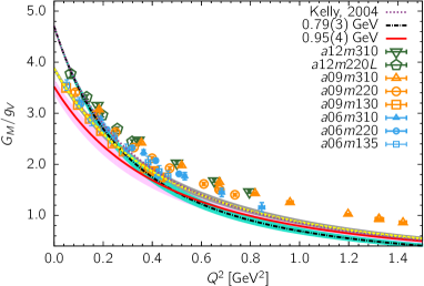
(a) 2-state

(b) $3^{\ast}$-state

Figure 4: Data for the normalized magnetic form factor ${G}_{M}/g_{V}$ for the 8 ensembles. The yellow dashed line is the dipole fit data extrapolated using only a fit in $m_{\pi}^{2}$. The rest is the same as in Fig. 3.

The $z-$expansion fits to $G_{M}(Q^{2})$ are much less stable since the point $F_{2}(Q^{2}=0)$ cannot be extracted from Eq. (4); it is obtained from the fit in $Q^{2}$. As a result, the $z-$expansion estimates in Table 4 are only with terms up to $z^{3}$. Results of fits with sumrules are even less stable and not presented here. Using the data from the 8 ensembles, we perform the continuum-chiral extrapolations for the magnetic charge radius $r_{M}$ and the magnetic moment $\mu$ using the ansatz:

$$\langle r_{M}^{2}\rangle(a,M_{\pi},L)=c_{1}^{M}+c_{2}^{M}a+c_{3}^{M}/M_{\pi}+c_{4}^{M}/M_{\pi}\exp(-M_{\pi}L)\,,$$ (8)

$$\mu(a,M_{\pi},L)=c_{1}^{\mu}+c_{2}^{\mu}a+c_{3}^{\mu}M_{\pi}+c_{4}^{\mu}M_{\pi}\left(1-\frac{2}{M_{\pi}L}\right)\exp(-M_{\pi}L)\,.$$ (9)

The form of the chiral and FV correction terms in $\langle r_{M}^{2}\rangle$ are taken from Ref. Bernard:1998gv . The FV term in $\mu$ is taken from Ref. Beane:2004tw . The NLO chiral correction in $\mu$ has a known coefficient, $(g_{A}^{2}M_{N})/(4\pi F_{\pi}^{2})M_{\pi}(1+(3M_{\pi})/(M_{N})\ln(M_{\pi}^{2}/\lambda^{2}))$ Meissner:1997hn , however, there is an additional chiral log at the same order, i.e., proportional to $M_{\pi}^{2}$, that involves unknown LEC. To include both chiral logs, an additional parameter is needed. Since we have data over a limited range of $M_{\pi}^{2}$ and with essentially three values of $M_{\pi}^{2}$, we neglect the chiral log corrections. For the same reason, we also leave $c_{3}^{\mu}$ a free parameter rather than take the form predicted by $\chi$PT. The results of the fits, with and without the respective FV correction term, are summarized in Table 4.

Table 4: Results of fits for the mean square magnetic charge radius $\langle r_{M}^{2}\rangle$ using Eq. 8 (upper half), and for $\mu$ using Eq. 9 (lower half). The second column shows the terms included in the chiral continuum extrapolation. The rest is the same as in Table 2.

		$2$-state			$3^{\ast}$-state
		dipole	$z^{2}$	$z^{3}$	dipole	$z^{2}$	$z^{3}$
$\langle r_{M}^{2}\rangle$	$a$, $M_{\pi}^{-1}$, FV	0.517(46)	0.716(96)	0.994(405)	0.587(68)	0.666(136)	0.878(649)
	$a$, $M_{\pi}^{-1}$	0.468(26)	0.619(60)	0.483(278)	0.477(39)	0.591(093)	0.580(439)
$\mu$	$a$, $M_{\pi}$, FV	3.52(15)	3.39(19)	3.72(42)	3.72(23)	3.39(30)	3.92(70)
	$a$, $M_{\pi}$	3.48(10)	3.41(13)	3.34(30)	3.64(14)	3.49(20)	3.63(46)

Our final results collected in Table 5, are obtained by fitting $\langle r_{M}^{2}\rangle$ and $\mu$ using Eq. (8) and Eq. (9), respectively, and keeping all four terms. For the $z-$expansion, we take a weighted average of the $z^{2}$ and $z^{3}$ truncation results. Estimates from the $2-$ and $3^{\ast}$-state fits are consistent for both the dipole and the $z$-expansion ansatz, but with larger errors than in $\langle r_{E}^{2}\rangle$. The $z$-expansion gives larger central values and errors compared to the dipole fits. The dipole estimates are smaller than the experimental value $r_{M}=0.86(3)\,\mathrm{fm}$ Mohr:2015ccw obtained from electron scattering experiments but the $z$-expansion estimates are consistent with the experimental value. Nevertheless, all four estimates of $\mu$ are $3/4$ of the precisely known value $\mu=1+\kappa_{p}-\kappa_{n}=4.7058$ with the anomalous magnetic moments of proton $\kappa_{p}=1.7928$ and of the neutron $\kappa_{n}=-1.9130$ Patrignani:2016xqp .

In Fig. 5, we plot the data and compare the chiral continuum extrapolation of $\langle r_{M}^{2}\rangle$ and $\mu$ for the $z^{2}$ fit to the data from the $3^{\ast}$-state analysis for two cases. The pink band shows the 4-parameter fit using Eqs. (8) and (9) projected on to the $M_{\pi}^{2}$ axis, i.e., fit to the data extrapolated to their continuum values in the other two variables, $a$ and $M_{\pi}L$. The grey band shows the fit only versus $M_{\pi}^{2}$, i.e., neglecting lattice spacing and volume dependence by setting $c_{2}^{M}=c_{4}^{M}=0$. The plots show that for a given pion mass, both $\langle r_{M}^{2}\rangle$ and $\mu$ decrease as the lattice spacing decreases. The fit keeping all four terms in Eqs. (8) and (9) is sensitive to this trend and thus gives smaller estimates. Ignoring the $a$ dependence, the fit versus just $M_{\pi}^{2}$ is controlled by the three 0.09 $\mathrm{fm}$ ensemble points as they have the smallest errors. It gives $\langle r_{M}^{2}\rangle=0.74(7)$, which fortuitously agrees with the experimental value $\langle r_{M}^{2}\rangle=0.74(5)$. However, the corresponding estimate of $\mu=4.11(9)$ is still lower than the experimental value $\mu=4.7058$.

Overall, it is the 0.06 $\mathrm{fm}$ data that controls the large negative slope in the lattice spacing dependence and leads to an underestimate of both $\langle r_{M}^{2}\rangle$ and $\mu$. Since the statistical errors in the data from these three 0.06 $\mathrm{fm}$ ensembles are the largest, reducing them will be the focus of future work.

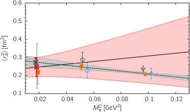
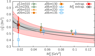
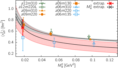
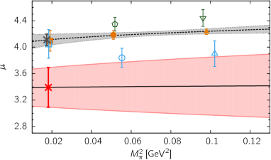
Figure 5: Chiral continuum extrapolation of $\langle r_{A}^{2}\rangle$, $\langle r_{E}^{2}\rangle$, $\langle r_{M}^{2}\rangle$, and $\mu$. The eight data points are obtained from the $3^{\ast}$-state fit for all four quantities, followed by $z^{2+4}$ fit for $G_{A}(Q^{2})$ and $G_{E}(Q^{2})$, and $z^{2}$ fit for $\langle r_{M}^{2}\rangle$ and $\mu$. The black solid line within the red error band shows the extrapolation using Eq. (3) for $\langle r_{A}^{2}\rangle$, Eq. (7) for $\langle r_{E}^{2}\rangle$, Eq. (8) for $\langle r_{M}^{2}\rangle$ and Eq. (9) for $\mu$. These 4-parameter fits (shown versus only $M_{\pi}^{2}$) are compared with a fit versus only $M_{\pi}^{2}$ (setting $c_{2,4}^{X}=0$ where $(X=A,E,M,\mu)$) shown by the black dashed line within the gray error band. The red and black crosses at $M_{\pi}=135$ MeV are the final estimates from these 4 versus 2 parameter fits.

Table 5: Final results for the isovector charge radii $r_{A},r_{E}$ and $r_{M}$ in unit of $\mathrm{fm}$ and the corresponding masses $\mathcal{M}_{A},\mathcal{M}_{E}$ and $\mathcal{M}_{M}$ in unit of $\mathrm{GeV}$. The magnetic moment $\mu_{p-n}\equiv 1+\kappa_{p}-\kappa_{n}$. The results are presented separately for the 2- and $3^{\ast}$-state fits used to control the excited-state contamination and the dipole and the $z-$expansion fits to capture the $Q^{2}$ behavior.

$Q^{2}$	3-pt.	$r_{A}$	$\mathcal{M}_{A}$	$r_{E}$	$\mathcal{M}_{E}$	$r_{M}$	$\mathcal{M}_{M}$	$\mu_{p-n}$
$z$-exp.	$2^{\phantom{\ast}}$	0.44(5)	1.56(18)	0.70(7)	0.98(10)	0.86(07)	0.80(06)	3.45(23)
	$3^{\ast}$	0.50(6)	1.36(17)	0.83(9)	0.82(08)	0.82(10)	0.83(10)	3.47(36)
dipole	$2^{\phantom{\ast}}$	0.46(2)	1.50(07)	0.69(2)	0.99(03)	0.72(03)	0.95(04)	3.52(15)
	$3^{\ast}$	0.51(2)	1.34(06)	0.79(3)	0.87(03)	0.77(04)	0.89(05)	3.72(23)

6 Summary

We have improved the control over excited-state contamination in the form factor analysis by including the second excite state in the fits. The results for $r_{A}$ and $r_{E}$ from the $3^{\ast}$-state fits are closer to the phenomenological value for both the $z$-expansion and the dipole analysis. The $3^{\ast}$-state fits are about $1\sigma$ ($3\sigma$) larger for the $z$-expansion (dipole) fit compared to the corresponding 2-state fit analysis.

The error from the dipole fits is typically a factor of 2–3 smaller than that from the $z$-expansion fits as shown in Table 5. Given the change in the value between 2- and $3^{\ast}$-state fits, we consider the error estimates using the $z$-expansion more realistic.

The $z$-expansion with $3^{\ast}$-state fits give an $r_{A}=0.50(6)\,\mathrm{fm}$ that is smaller than the phenomenological estimate $r_{A}=0.68(16)\,\mathrm{fm}$ Meyer:2016oeg . The results for $r_{E}=0.83(9)\,\mathrm{fm}$ and $r_{M}=0.82(10)\,\mathrm{fm}$ are consistent with phenomenological values $r_{E}=0.8409(4)\,\mathrm{fm}$ and $r_{M}=0.86(3)\,\mathrm{fm}$. The outlier is our estimate of the magnetic moment $\mu$ which is about $3/4$ of the precisely known experimental value $\mu=4.7058$.

Our plan for the future is to increase the statistics on the two physical pion mass ensembles and understand why the data for the three form factors $G_{A}$, $\tilde{G}_{P}$ and $G_{P}$ do not satisfy the axial Ward identity.

Acknowledgement We thank the MILC Collaboration for providing the 2+1+1-flavor HISQ lattices. We thank Emanuele Mereghetti for discussions. Simulations were carried out on computer facilities of (i) the USQCD Collaboration, which are funded by the Office of Science of the U.S. Department of Energy, (ii) the National Energy Research Scientific Computing Center, a DOE Office of Science User Facility supported by the Office of Science of the U.S. Department of Energy under Contract No. DE-AC02-05CH11231; (iii) Oak Ridge Leadership Computing Facility at the Oak Ridge National Laboratory, which is supported by the Office of Science of the U.S. Department of Energy under Contract No. DE-AC05- 00OR22725; (iv) Institutional Computing at Los Alamos National Laboratory; and (v) the High Performance Computing Center at Michigan State University. The calculations used the Chroma software suite Edwards:2004sx . This work is supported by the U.S. Department of Energy, Office of Science of High Energy Physics under contract number DE-KA-1401020 and the LANL LDRD program. The work of H-W. Lin was supported in part by the M. Hildred Blewett Fellowship of the American Physical Society.

References

- (1) R. Gupta, Y.C. Jang, H.W. Lin, B. Yoon, B. Bhattacharya (2017), 1705.06834
- (2) A.A. Aguilar-Arevalo et al. (MiniBooNE), Phys. Rev. D81, 092005 (2010), 1002.2680
- (3) V. Bernard, H.W. Fearing, T.R. Hemmert, U.G. Meissner, Nucl. Phys. A635, 121 (1998), [Erratum: Nucl. Phys.A642,563(1998)], hep-ph/9801297
- (4) A.S. Meyer, M. Betancourt, R. Gran, R.J. Hill, Phys. Rev. D93, 113015 (2016), 1603.03048
- (5) V. Bernard, L. Elouadrhiri, U.G. Meissner, J. Phys. G28, R1 (2002), hep-ph/0107088
- (6) M. Gockeler, T.R. Hemmert, R. Horsley, D. Pleiter, P.E.L. Rakow, A. Schafer, G. Schierholz (QCDSF), Phys. Rev. D71, 034508 (2005), hep-lat/0303019
- (7) P.J. Mohr, D.B. Newell, B.N. Taylor, Rev. Mod. Phys. 88, 035009 (2016), 1507.07956
- (8) A. Antognini et al., EPJ Web Conf. 113, 01006 (2016), 1509.03235
- (9) S.R. Beane, Phys. Rev. D70, 034507 (2004), hep-lat/0403015
- (10) U.G. Meissner, S. Steininger, Nucl. Phys. B499, 349 (1997), hep-ph/9701260
- (11) C. Patrignani et al. (Particle Data Group), Chin. Phys. C40, 100001 (2016)
- (12) R.G. Edwards, B. Joo (SciDAC Collaboration, LHPC Collaboration, UKQCD Collaboration), Nucl.Phys.Proc.Suppl. 140, 832 (2005), hep-lat/0409003