Binder migration during drying of lithium-ion battery electrodes: modelling and comparison to experiment

Abstract

The drying process is a crucial step in electrode manufacture as it can affect the component distribution within the electrode. Phenomena such as binder migration can have negative effects in the form of poor cell performance (e.g. capacity fade) or mechanical failure (e.g. electrode delamination from the current collector). We present a mathematical model that tracks the evolution of the binder concentration in the electrode during drying. Solutions to the model predict that low drying rates lead to a favourable homogeneous binder profile across the electrode film, whereas high drying rates result in an unfavourable accumulation of binder near the evaporation surface. These results show strong qualitative agreement with experimental observations and provide a cogent explanation for why fast drying conditions result in poorly performing electrodes. Finally, we provide some guidelines on how the drying process could be optimised to offer relatively short drying times whilst simultaneously maintaining a roughly homogeneous binder distribution.

1 Introduction

Lithium-ion batteries are currently used to power the vast majority of portable electronic devices, such as cell-phones, laptops, and tablets, and are growing in popularity for use in hybrid and electric vehicle propulsion [19]. While one of the biggest challenges in lithium-ion battery research is to increase the energy density of batteries, another equally important challenge is to optimize the manufacturing process to improve long-term cycling performance and capacity lifetime while keeping control of the manufacturing costs [5, 17, 27]. One particularly sensitive step in cell production that determines the final quality of the battery pack is the manufacturing process for the electrodes [29, 14].

Typically, electrodes are manufactured by coating a current collector with a slurry mixture comprised of active material (AM) particles, conductive carbon nanoparticles, polymer binder (commonly polyvinylidene fluoride (PVDF)) and solvent (commonly N-Methyl-2-pyrrolidone (NMP)) [15, 18, 29, 14]. This mixture is then dried (i.e. the solvent is evaporated) by exposure to air flow, heat and sometimes a reduction in ambient pressure [29, 14, 1, 26]. The mixture preparation and coating steps previous to drying are very important and have to be carefully executed to ensure that electrodes are manufactured properly. For instance, it has been shown that slurry mixtures prepared by a multi-step process lead to a more uniform distribution of AM and carbon particles, resulting in significantly less electrode polarization and better cycling capability [15, 18]. For an extensive review on mixture preparation the reader is referred to [16].

The most frequently used coating method in industry is slot-die coating, in which a liquid is poured into a die that deposits the coating liquid onto a rolling substrate belt. Coating defects such as film instability and edge effects can occur and need to be controlled which can, for example, be achieved by varying the coating speed and the gap ratio [24, 25]. In contrast, many research devices are manufactured by spreading the slurry on the substrate by hand using a doctor blade. The use of NMP as a solvent is also highly costly and replacing it with aqueous solutions would both reduce the cost of electrode production and be more environmental friendly [11].

Drying begins once the current collector has been coated with the wet particulate electrode mixture. The AM particles are in suspension in the mixture whilst the binder is dissolved in the solvent. The solvent starts evaporating from the top surface of the electrode film and the film begins to shrink. The film once the AM particles are in contact the film thickness stops decreasing, but evaporation continues and the pore space between particles starts emptying. When all the solvent has been removed the particles form a non-moving scaffold and the wet pore space has turned into dry pore space. This being said, some recent experimental results indicate that in some circumstances pore emptying onset even before the end of film shrinkage [12]. This part of the process has been subject of intense experimental research in recent years [29, 14, 1, 12, 6, 13, 21]. There is now a consensus that changes to the drying process parameters (temperature, air-flow and pressure) significantly affect the final electrode microstructure and, therefore, the electrochemical and mechanical properties of the resulting battery electrode. It has been observed by several experimental groups that high temperatures and drying rates lead to an accumulation of binder at the film evaporation surface and a corresponding depletion at the film-substrate interface [29, 1, 6, 21]. The consequence of binder inhomogeneities include lower adhesion of the electrode to the current collector [29, 14, 1], increased electrical resistivity [29] and decreased cell capacity [14]. Chou et al [2] conclude that even though binder makes up only a small fraction of the electrode composition, it plays a very important role in the cycling stability and rate capability of the electrode.

Investigation depletion and/or accumulation of binder in different regions of electrodes has been a matter of experimental investigation [14, 1, 13, 21]. In Jaiser et al [14] a “top-down” film consolidation process is suggested, in which a dense layer, or ‘crust’, appears on the drying surface and grows down until it reaches the substrate interface. However, a follow-up study seems to indicate that film shrinkage may occur in a more homogeneous fashion [13]. In both cases, it was found that removal of the solvent from the film surface causes enrichment of binder in the upper regions and that this upward transport cannot be compensated by diffusion if the drying rates are high. The effect of the drying temperature on the drying process is discussed in [1]. These results show that higher temperatures negatively influence electrode adhesion to the current collector due to binder depletion at the electrode-collector interface. The detrimental effect of high drying temperatures has been recently confirmed via energy dispersive x-ray spectroscopy in [21].

Theoretical models detailing the physical mechanisms governing the drying of a single-component colloidal suspension were studied in [28] while drying of polymer solutions was investigated in [8, 7]. However, to the best of our knowledge, the process of drying suspensions composed of colloidal particles and dissolved binders has not been tackled before. The aims of this work are to: (i) provide a mathematical model for such a situation, (ii) to compare the predictions of this model with experimental results, and (iii) use the model to suggest strategies to optimise the drying process. The rest of the paper is organized as follows. In the next section we formulate and solve a simple model for mass transport within an electrode when the colloidal suspension of the AM particles is stable and the particles remain separated and distributed homogeneously until full consolidation has occurred. We then formulate the model for the transport of binder through the drying film and present estimates for the parameters in the model. In the next section, §3, we present both numerical and approximate (asymptotic) solutions of the model for different drying rates and protocols. Finally, in §4 we draw our conclusions.

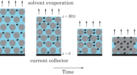
Figure 1: Illustration of the drying process of an electrode film sitting on top of a current collector. The blue background represents the solvent (which evaporates from the top surface of the film), and the black and grey particles represent the polymer binder and AM particles respectively.

2 Problem formulation

We formulate a one-dimensional model in which mass transfer occurs only in the $z$-direction (perpendicular to the substrate). All model equations are defined for $z\in[0,H(t)]$, where $H(t)$ is the time-dependent position of the top of the electrode film, see Figure 1. The assumption that the model is one-dimensional is justified by the fact that the electrode film is slender, i.e. its lateral extent is much larger than its thickness (height). We will track two material phases: a liquid phase (comprised of both the solvent and dissolved binder), with volume fraction $\phi_{\text{l}}$, and a solid phase (AM particles), with volume fraction $\phi_{\text{s}}$. We begin by presenting some scaling arguments that aim to identify the important effects at play during drying.

First, we characterise the typical time required for an AM particle to settle through the NMP film. Using the material properties of the NMP solvent and the graphite active material collected in Table 1 together with an estimate of the typical viscosity of NMP at 348K of $\eta=1.65$mPa s [9], we can estimate a time scale for sedimentation of a small 5$\mu$m graphite AM particle through a 120$\mu$m NMP film of around 10s, which is very much faster than the typical drying time of around 1 minute (note that larger particles sediment even more quickly). It is therefore apparent that the flows resulting from the drying process cannot lead to significant AM particle redistribution within the film (the gravitational buoyancy forces always dominate the drag forces from the drying flows). Furthermore, experimental evidence presented in [13] indicates that AM particle distribution within the film is uniform throughout the drying process which, in turn, suggests that there is another physical force dominant over both buoyancy and drag forces. This we believe to be a repulsive colloidal force resulting from charge on the AM particles. Henceforth, in line with data presented in [13], we assume that AM particles are always uniformly distributed within the film.

It remains to specify a model for the transport of the PVDF binder particles. These particles are typically very small, with a hydrodynamic radius of around 15nm [22], and therefore are largely unaffected by gravitational buoyancy effects over the drying time of the film. Nevertheless, it seems conceivable that they may be affected by colloidal forces. In order to counter this hypothesis, we note firstly that PVDF is an inert polymer, and so unlikely to be charged, and secondly that experiments conducted in [14] show that distribution of binder is strongly dependent on drying rate, refuting the hypothesis that PVDF forms a stabilised colloidal suspension in NMP. We therefore model transport of PVDF within the NMP solvent by an advection diffusion equation in order to include both the effect of the drying flows and thermal diffusion on the motion of PVDF particles. Changes in the macroscopic (effective) diffusivity of the binder (caused by changes in the volume fractions of the different phases through the film) will be accounted for via use of the Bruggemann approximation [3]. Finally, we note that crystallisation only begins to occur when the mass fraction of the binder reaches 77 wt% at 60^oC (or larger for higher temperatures) [20]. The parameters in Table 1 indicate that these concentrations will likely not occur during the stages of the drying process under consideration here, see the discussion at the end of §2.2. Crystallisation effects are therefore neglected.

The model will be formulated in two parts. First, we will construct the model for the mass transport of the liquid phase (dissolved binder and solvent) and solid phase (AM particles). Then, we will obtain the equations describing the advection and diffusion of binder through the moving solvent. We can adopt this approach because the volume fraction of the binder is so small (typically only 0.01–0.05 [18, 29, 14, 13]) that, to a good approximation, the binder concentration does not influence the mass transport of the liquid and solid phases. However, the advection-diffusion model for the binder concentration can only be solved with knowledge of the solvent flow. This suggests a two-step solution process in which we first solve for particle and solvent flow and then use the results obtained as input to the binder transport model. Finally, we solve this model to obtain the evolution of the binder concentration.

2.1 Mass transport

Conservation equations for the mass of the solid (AM particles) and liquid (binder and solvent) phases expressed in terms of their respective volume fractions have the form

$$\frac{\partial\phi_{\text{s}}}{\partial t}+\frac{\partial F_{\text{s}}}{\partial z} =0,$$ (1a)

$$\frac{\partial\phi_{\text{l}}}{\partial t}+\frac{\partial F_{\text{l}}}{\partial z} =0,$$ (1b)

where $F_{\text{l}}$ and $F_{\text{s}}$ are the volume fraction fluxes (with dimensions of m/s) of the solid and liquid phases, respectively. In turn, these are related to the volume averaged velocities in each phase via

$$F_{\text{s}} =v_{\text{s}}\phi_{\text{s}},$$ (2a)

$$F_{\text{l}} =v_{\text{l}}\phi_{\text{l}}.$$ (2b)

Since there are only two phases (liquid and solid) their volume fractions sum to one, i.e.

$$\phi_{\text{s}}+\phi_{\text{l}}=1.$$ (3)

As drying proceeds and liquid is removed from the slurry, the resulting dynamics will depend on the stability of the homogeneous state of the suspension. This is described by the widely accepted Derjaguin-Landau-Verwey-Overbeek (DLVO) theory [10] in which the force between two spherical particles is comprised of two contributing parts; relatively long-range Coulombic repulsion, that is screened by a counterion cloud, and short-range van der Waals attraction. If the repulsive electrostatic barrier is weak, then as solvent is removed and particles are forced into closer vicinity, they will quickly begin to aggregate forming a crust [4]. In contrast, if the repulsive barrier is strong (as it is here), then particles will remain well-separated until the volume of the film has been reduced so much that they are forced into contact. In the latter case, the suspension is stable and the solid phase is forced to be homogeneously distributed throughout the electrode film (as seen in [13]), i.e. we have

$$\phi_{\text{s}}=\phi_{\text{s}}(t)\,,$$ (4)

.

The equations above are solved subject to no-flux boundary conditions on the current collector, namely,

$$F_{\text{s}}|_{z=0} =0,$$ (5a)

$$F_{\text{l}}|_{z=0} =0,$$ (5b)

and the following flux conditions on the evaporation surface $z=H(t)$:

$$\frac{D_{\text{s}}}{Dt}(z-H)\Big{|}_{z=H(t)}=0\qquad\Longrightarrow\qquad-\dot{H}+ v_{\text{s}}\Big{|}_{z=H(t)}=0,$$ (6)

$$\frac{D_{\text{l}}}{Dt}(z-H)\Big{|}_{z=H(t)}=\frac{\gamma}{\phi_{\text{l}}}\Big{|}_{z=H(t)}\qquad\Longrightarrow\qquad-\dot{H}+ v_{\text{l}}\Big{|}_{z=H(t)}=\frac{\gamma}{\phi_{\text{l}}}\Big{|}_{z=H(t)},$$ (7)

which represent zero-flux of the solid phase and an evaporation flux $\gamma$ of the liquid phase, respectively, through the surface $z=H(t)$. In (6) and (7) the operators $D_{\text{s}}/Dt$ and $D_{\text{l}}/Dt$ are material derivatives taken with respect to the solid and liquid velocities, respectively, and a dot indicates a derivative with respect to time. At the beginning of the drying process we assume that the two phases are well mixed and are present in the following proportions

$$\phi_{\text{s}}|_{t=0} =\phi_{\text{s}}^{0},$$ (8a)

$$\phi_{\text{l}}|_{t=0} =1-\phi_{\text{s}}^{0},$$ (8b)

whilst the film is taken to have initial thickness

$$H|_{t=0}=H_{0}.$$ (9)

Validity of the model terminates at the time $t_{\text{end}}$ when the AM particles are consolidated (i.e. they make direct contact with each other) and the liquid surface begins to intrude into the scaffold formed by the electrode particles. We define the solid volume fraction at this fully consolidated stage to be $\phi_{\text{s}}^{\text{max}}=\phi_{\text{s}}(t_{\text{end}})$ and model solutions will be terminated when this state is reached.

Summing equations (1a)–(1b), using (3), integrating with respect to $z$ and imposing the boundary conditions (5) reveals that

$$F_{\text{l}}+F_{\text{s}}=0.$$ (10)

Substituting the above into the sum of the boundary conditions (6) and (7), and using (2) and (3), gives the following evolution equation for the position of the top surface of the film

$$\dot{H}=-\gamma.$$ (11)

This result can readily be interpreted as global mass conservation throughout the film.

As illustrated in Figure 1, the solid volume fraction is space-independent because of strong repulsion between AM particles. Thus, equation (1a) can be integrated with respect to $z$ and (5a) imposed to give

$$F_{\text{s}}=-\dot{\phi}_{\text{s}}z.$$ (12)

Eliminating $F_{\text{s}}$ from the above in favour of $v_{\text{s}}$ using (2a) and using the boundary condition (6) gives $d/dt(H\phi_{\text{s}})=0$. This can be integrated and the initial conditions (8a) and (9) imposed to give $\phi_{\text{s}}=H_{0}\phi^{0}_{\text{s}}/H$. Back substitution of this result into (12), then using (10) and (11) gives the following expressions for the volume fractions and volume-averaged fluxes

$$\begin{split}\phi_{\text{s}}=\frac{\phi_{\text{s}}^{0}H_{0}}{H},\quad\phi_{\text{l}}=1-\frac{\phi_{\text{s}}^{0}H_{0}}{H},\quad F_{\text{s}}=-\frac{\gamma\phi_{\text{s}}^{0}H_{0}}{H^{2}}z,\quad F_{\text{l}}=\frac{\gamma\phi_{\text{s}}^{0}H_{0}}{H^{2}}z\,.\end{split}$$ (13)

2.2 Binder transport

The polymer binder is distributed within the liquid phase only, thus, a volume-averaged continuity equation describing the concentration $c$ of dissolved binder in the solvent is

$$\frac{\partial}{\partial t}\left(\phi_{\text{l}}c\right)+\frac{\partial J}{\partial z}=0,\qquad J=F_{\text{l}}c-D_{\text{eff}}\frac{\partial c}{\partial z},$$ (14)

where $J$ is the volume-averaged mass flux of dissolved binder. This flux is composed of two parts: an advective part with the volume-averaged velocity of the solvent and a diffusive part with an “effective” diffusion coefficient $D_{\text{eff}}$. We estimate this effective diffusivity using the Bruggemann approximation which assumes that $D_{\text{eff}}=D\phi_{\text{l}}^{3/2}$, where $D$ is the diffusivity of the binder in the solvent [3]. So, the value of $D_{\text{eff}}$ changes during the drying process as $\phi_{\text{l}}$ varies according to (13).

Suitable boundary conditions on (14) require that there is zero flux of binder through both the current collector and the free surface $z=H(t)$. We therefore have

$$J|_{z=0}=0,\qquad J|_{z=H(t)}=\phi_{\text{l}}c\frac{dH}{dt}.$$ (15)

One can verify using the boundary conditions (15) and Leibniz integral rule on (14) that the total amount of binder in the film $\int_{0}^{H(t)}c\phi_{\text{l}}\,dz$ is conserved throughout the drying process. We assume that initially the binder is homogeneously distributed throughout the solvent. Thus, a suitable initial condition to close (14) is

$$c|_{t=0}=c_{0}.$$ (16)

It should be noted that the model presented here is only valid until binder concentrations get large enough that the PVDF begins to crystallize out of solution. At 60 ^oC the mass fraction for crystallization of PVDF from NMP is 77 wt% and this value increases with temperature [20]. As a reference for the parameter estimation we will take values from [14, 13] where drying was performed at 76.5 ^oC, so we expect mass fraction for crystallization to be slightly above 77 wt%. As we will show later, in §3.3, these concentrations are only achieved under extremely aggressive drying rates.

2.3 Parameter estimates

We calibrate simulations using the data provided in [14, 13] and summarised here in Table 1. We find that the initial volume fraction of the solid electrode particles is

$$\phi_{\text{s}}^{0}=\frac{\omega_{\text{s}}^{0}}{\rho_{\text{s}}}\left(\frac{\omega_{\text{s}}^{0}}{\rho_{\text{s}}}+\frac{\omega_{\text{b}}^{0}}{\rho_{\text{b}}}+\frac{\omega_{\text{NMP}}^{0}}{\rho_{\text{NMP}}}\right)^{-1}\approx 0.2792\,.$$ (17)

where the subscripts “s”, “b” and “NMP” indicate solid electrode particles, binder and solvent, respectively. To compute the final (and maximal) value of the solid volume fraction we also make use of the measured porosity of the dried electrode film $p=0.46$ [13] and find that

$$\phi_{\text{s}}^{\text{max}}=(1-p)\frac{\omega_{\text{s}}^{\text{max}}}{\rho_{\text{s}}}\left(\frac{\omega_{\text{s}}^{\text{max}}}{\rho_{\text{s}}}+\frac{\omega_{\text{b}}^{\text{max}}}{\rho_{\text{b}}}+\frac{\omega_{\text{NMP}}^{0}}{\rho_{\text{NMP}}}\right)^{-1}\approx 0.5032\,.$$ (18)

The initial concentration of binder in the solvent and film thickness are

$$c_{0}=\frac{\tilde{c}_{0}}{(1-\phi_{\text{s}}^{0})}\approx 56.95\,\text{kg/}\text{m}^{3},\quad H_{0}\approx 114\,\mu\text{m},$$ (19)

where $\tilde{c}_{0}=\rho w_{\text{b}}^{0}=41.05$ kg/m³ with $\rho=\rho_{\text{s}}w_{\text{s}}^{0}+\rho_{\text{b}}w_{\text{b}}^{0}+\rho_{\text{NMP}}w_{\text{NMP}}^{0}$ is the initial concentration of binder in the film [14, 12, 13]. In the subsequent section we will consider how the dynamics change with varying drying rate. Nonetheless, we note that a typical value of the mass flux across the evaporation surface is $q_{\text{s}}=1.19$ g m^-2 s^-1 [14, 12, 13], so that a typical value for $\gamma$ is given by

$$\gamma=\frac{q_{\text{s}}}{\rho_{\text{NMP}}}\approx 1.16\,\mu\mbox{m s}^{-1}.$$ (20)

As a reference for the diffusion coefficient we will use $D=1.14\cdot 10^{-10}$ m²/s which is obtained, as described in the supplementary information, by qualitatively matching the solution of our model to the experimental results presented in [14]. If we consider the viscosity of NMP $\eta=1.65$ mPa s and a temperature $T=348$ K, the estimate for the hydrodynamic radius of a PVDF particle using the Stokes-Einstein relation is $R_{H}=k_{B}T/6\pi\eta D=2.48$ nm, which is close to the hydrodynamic radius found experimentally for PVDF chains in PVDF/Propylene-carbonate mixtures at low concentrations, $R_{H}\approx 15$ nm [22]. At high concentrations, $R_{H}$ is found to increase and stabilize at around 200-300 nm, which results in the decrease of the PVDF diffusivity [23, 22]. To keep the formulation of the problem tractable, we do not account for dependence of the diffusivity on the concentration of PVDF and keep the value of the diffusion coefficient fixed at $D=1.14\cdot 10^{-10}$ m²/s.

Material	$\rho$ (g/cm3)	$\omega^{0}$	$\omega^{\text{max}}$
Solvent (NMP)	1.03	0.526	0
Polymer binder (PVDF)	1.76	0.026	0.055
Graphite particles	2.21	0.449	0.945

Table 1: Typical densities $\rho$ for electrode film components and initial and final mass fractions, respectively, $\omega^{0}$ and $\omega^{\text{max}}$, for the electrode components used in Jaiser et al [14, 13]. As noted previously, we do not account for the contribution of carbon black into our model, thus its mass fraction ($w_{cb}=0.014$ [14, 13]) has been added to the mass fraction of graphite particles.

3 Results and discussion

In this section we first present and contrast typical model solutions for both high and low drying rates. Then, we reproduce the experimental procedure followed in [14] and demonstrate good agreement between model solutions and experimental results. Finally, we examine the effects of allowing time-dependent drying rates and consider how this can be used to devise possible strategies to optimize the drying process.

3.1 Low and high drying rate limits

The evolution of the binder distribution in a stable colloid is determined by solving (14)-(16) where the phase volume fractions and fluxes are given by (13). Although no exact solutions to this problem are available, we can solve the problem approximately in two different ways: (i) using matched asymptotic expansions valid for limiting values of the Peclet number $Pe=\gamma H_{0}/D$ (measuring the relative strength of advection to diffusive transport), and; (ii) using a numerical scheme based on the finite differences. We will contrast the two distinct limiting cases where $Pe\ll 1$ or $Pe\gg 1$ which we will henceforth refer to as the low drying rate (LDR) or high drying rate (HDR) case, respectively. Details on the derivation of the asymptotic solutions and the numerical scheme can be found in the supplementary information.

In the LDR limit ($Pe\ll 1$) the concentration of binder is well approximated by

$$\frac{c(z,t)}{c_{0}}\approx\frac{(1-\phi_{\text{s}}^{0})}{(\frac{H}{H_{0}}-\phi_{\text{s}}^{0})}+Pe\frac{(1-\phi_{\text{s}}^{0})}{(\frac{H}{H_{0}}-\phi_{\text{s}}^{0})^{2}\phi_{\text{l}}(t)^{1/2}}\left(\frac{z^{2}}{2H_{0}^{2}}-\frac{H^{2}}{6H_{0}^{2}}\right)\,.$$ (21)

where $H(t)=H_{0}-\gamma t$ (obtained after integrating (11)). In the HDR limit the concentration of binder is approximately given by

$$\frac{c(z,t)}{c_{0}}\approx 1+A(t)\exp\left(-\frac{Pe(H-z)}{H_{0}\phi_{\text{l}}(t)^{3/2}}\right)\,,$$ (22)

where now the time-dependent constant of integration $A(t)$ is the solution of the following initial-value problem

$$\dot{A}=-\frac{5}{2}A\frac{\dot{\phi}_{\text{l}}(t)}{\phi_{\text{l}}(t)}+\frac{Pe}{\phi_{\text{l}}(t)^{3/2}}\,,\qquad A(0)=1\,.$$ (23)

In Figure 2 we present typical solutions for both a low and high drying rate by taking $\gamma=1.25\cdot 10^{-7}$ m s^-1 ($Pe\approx 0.1$) and $\gamma=1.25\cdot 10^{-5}$ m s^-1 ($Pe\approx 10$), respectively. The red solid lines correspond to the asymptotic solutions (21)–(52) and blue dashed lines to numerical solutions (see the supplementary information for details). The two solution approaches exhibit very favourable agreement despite the moderate sizes of the Peclet number used in each case thereby validating both approaches. In panel (a) (low drying rate) the concentration of binder progressively increases as solvent evaporates with the distribution remaining almost homogeneous throughout the whole drying process. For low drying rates ($Pe\ll 1$) the drying time is relatively large and the velocity of the solvent (upward) relatively small. Thus, advection is only able to induce small gradients in the binder concentration and the diffusive process has a long time to act to smooth out these gradients. The final binder distribution is therefore relatively uniform. This is reflected in the asymptotic solution (21) where the leading order term (and most dominant) is a function of time only and the dependence in $z$ introduced only at the next order. Contrastingly, in Figure 2(b) (high drying rate), the drying time is relatively small and the velocity of the solvent relatively large. Here, diffusion has less time to dissipate concentration gradients induced by solvent advection. As a result, binder accumulates near the top surface of the electrode film, which is captured by the exponential term in (53). We can therefore conclude that low drying rates lead to a favourable homogeneous binder profiles across the electrode film, whereas high drying rates tend to unfavourably accumulate the binder near the evaporation top surface.

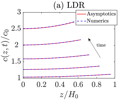
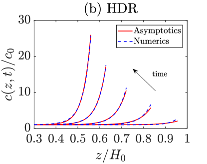
Figure 2: Numerical and asymptotic solutions of the binder transport model (14)-(16). Panel (a) shows concentration profiles corresponding to a low drying rate ($\gamma=1.25\cdot 10^{-7}$ m s^-1) for five values of time between 39.8 s and 401.92 s. Panel (b) shows concentration profiles corresponding to a high drying rate ($\gamma=1.25\cdot 10^{-5}$ m s^-1) for five values of time between 0.4 s and 4.02 s. The last profile in (a) and (b) corresponds to the concentration profile at the end of drying $t=t_{\text{end}}$. Note that panel (b) has been truncated at $z=0.3$ for ease of viewing; the solution for $z<0.3$ is essentially flat.

3.2 Agreement with experiment

We now utilise the model to reproduce and elucidate the experimental results obtained in Jaiser et al [14]. In their work electrode films were first dried at a high drying rate for a given period of time $[0,t_{\text{trans}}]$. The drying rate was then decreased and the drying process continued until the film was completely dry. The main result in their study was a plot of $c_{\text{top}}=c|_{z=H,t=t_{end}}$ and $c_{\text{bot}}=c|_{z=0,t=t_{end}}$ against $t_{\text{trans}}$, i.e. the binder concentrations at the top (evaporation surface) and bottom (current collector) of the electrode at the end of the drying process $t=t_{\text{end}}$. They observed that: (i) $c_{\text{top}}$ and $c_{\text{bot}}$ are almost constant for sufficiently small $t_{\text{trans}}$, (ii) there is then a small range of values of $t_{\text{trans}}$ where $c_{\text{top}}$ increases whereas $c_{\text{bot}}$ decreases beyond which, (iii) $c_{\text{top}}$ and $c_{\text{bot}}$ once again saturate to constant values. We reproduce this protocol in our model by taking the time-dependent drying rate used in [14], namely

$$\gamma(t)=\begin{dcases}1.16\,\mu\mbox{m}\,\mbox{s}^{-1}\quad(\mbox{Pe}=0.94)\quad\mbox{for}\quad t<t_{\text{trans}},\\ 0.51\,\mu\mbox{m}\,\mbox{s}^{-1}\quad(\mbox{Pe}=0.41)\quad\mbox{for}\quad t>t_{\text{trans}}.\end{dcases}$$ (24)

Figure 3 shows the values of $c_{\text{top}}$ and $c_{\text{bot}}$ for different choices of $t_{\text{trans}}$ as determined using the numerical procedure described in the supplementary information. The plots show how $c_{\text{top}}$ increases slowly until $t_{\text{trans}}\gamma/H_{0}\approx 0.34$ and then increases more rapidly until $t_{\text{trans}}\gamma/H_{0}\approx 0.44$. For even larger values of $t_{\text{trans}}$, the decrease in drying rate does not occur until after the electrode is completely dry, thus $c_{\text{top}}$ remains constant. The evolution of $c_{\text{bot}}$ behaves in an opposite fashion: it first decreases slowly until $t_{\text{trans}}\gamma/H_{0}\approx 0.34$, then decreases fast until $t_{\text{trans}}\gamma/H_{0}=t_{\text{end}}\gamma/H_{0}\approx 0.44$ and stays constant for $t_{\text{trans}}>t_{\text{end}}$. These results show strong qualitative agreement with those presented in Figure 6 from [14].

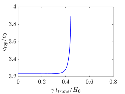
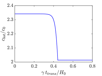
Figure 3: Normalized concentration of binder on top and bottom of the electrode at the end of drying as a function of the nondimensional transition time between high and low drying rate.

3.3 Identifying viable constant drying rates

We now use the model to identify the largest rate at which an electrode can afford to be dried without inducing unacceptably large gradients in the binder concentration. In Figure 4 we present the concentration of binder on top of the electrode at the end of drying as a function of the Peclet number. The value of the drying rate by which concentration gradients remain relatively small (i.e. $c_{\text{top}}$ does not increase substantially) corresponds to $Pe=\gamma H_{0}/D\lessapprox 1$. For the values of $H_{0}$ and $D$ estimated in §2.3 this yields $\gamma\lessapprox 1\cdot 10^{-6}$ m/s.

From Figure 4 we also see that, unless a very aggressive drying rate is used, it seems unlikely that crystallization of the PVDF will begin to occur until after the film is fully consolidated, the point at which our model is no longer valid and our simulations are terminated.

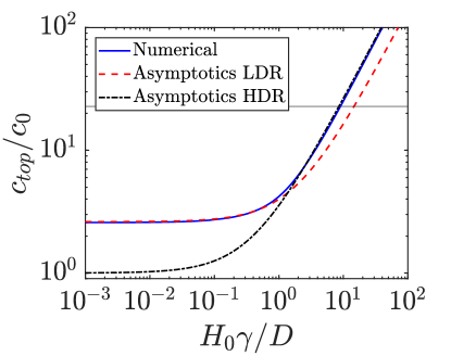
Figure 4: Binder concentration on top of the electrode at the end of drying as a function of the drying rate $\gamma$. The solid line corresponds to the numerical solution and the the dashed and dash-dotted lines correspond to the asymptotic solution for low and high drying rate, respectively. The horizontal line denotes the binder concentration at which crystallisation begins to occur at $T=60$ ^oC, corresponding to $c(z,t)/c_{0}=22.75$ [20], which represents an orientative upper bound for the concentration in our model.

3.4 Exploiting variable drying rates

As we have demonstrated, the drying process should be carried out slowly to prevent an undesirable accumulation of binder near the evaporation surface. However, from an industrial point of view, short drying processes are preferred in order to increase throughput [11]. The model is now used to investigate whether (and to what extent) allowing time-dependent drying rates can be helpful in simultaneously achieving more homogeneous binder distributions and shorter drying times. To do so, we consider three different drying protocols: (Case 1) a constant drying rate, (Case 2) a linearly increasing drying rate, and (Case 3) a linearly decreasing drying rate, as outlined below:

Case 1: $$\gamma(t) =\gamma_{0} \mbox{for}\quad 0\leq t\leq t_{end},$$ (25)

Case 2: $$\gamma(t) =2\gamma_{0}\frac{t}{t_{\text{end}}} \mbox{for}\quad 0\leq t\leq t_{end},$$ (26)

Case 3: $$\gamma(t) =2\gamma_{0}\left(1-\frac{t}{t_{\text{end}}}\right) \mbox{for}\quad 0\leq t\leq t_{end},$$ (27)

and select $\gamma_{0}=1.16$ $\mu\text{m}$ s^-1. Note that in defining (25)–(27) we have ensured that the time taken to fully consolidate the film, $t_{\text{end}}$, is the same in all three cases (see supplementary information). The evolution of the position of the evaporating surface is represented in Figure 5a. In Figure 5b we show the concentration of binder across the electrode at two different times during the drying process (near the beginning and at the end) for each choice of the drying rate.

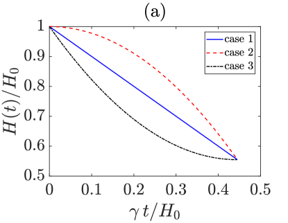
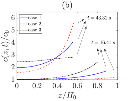
Figure 5: (a) Evolution of the position of the top surface for the three drying rates considered, cf. (25)–(27). (b) Concentration of binder near the beginning ($t=16.41$ s) and at the end ($t=43.31$ s) of the drying process for each case.

We observe that choosing a linearly decreasing drying rate (case 3) gives the most evenly distributed binder concentration whilst choosing a linearly increasing one yields the worst results. This suggests that, if the goal is obtaining an acceptably homogeneous distribution of binder and a short drying time, the best procedure is to dry the electrode at a high drying rate at the beginning and at a low drying rate near the end of the process. This can be rationalised by noting that even though large binder concentration gradients may be established by the initial high drying rate, so long as the rate is dropped towards the end of the process, diffusive effects overcome the upward convection of the solvent and have sufficient time to act to dissipate these inhomogeneities. These results, which have been obtained for a fixed drying time, can be interpreted in the sense of minimizing the drying time: approximately the same concentration of binder as obtained at a given constant drying rate could be achieved in a shorter time by using HDR at the beginning and LDR near the end. An interesting and open question concerns whether the drying process can be further optimised by allowing a more complicated time-dependent behaviour for $\gamma(t)$. Work to address this question is already underway and will be reported in a future study.

4 Conclusions

We have presented a mathematical model that predicts the mass transport and evolution of binder concentration during the drying of lithium-ion battery electrodes. We have found that higher drying rates tend to induce larger binder concentration gradients because to a combination of: (i) the more aggressive evaporation rates causing a larger (upward) convection of the binder solvent and; (ii) the decreasing drying time allows less opportunity for diffusion to redistribute the binder evenly throughout the film. We have demonstrated that the model satisfactorily reproduces recently published experimental results of binder migration phenomena during drying. Finally, we have shown that a sound strategy to reduce the drying time whilst simultaneously maintaining small variations in the binder concentration is to initially apply a period of high drying rate and to then decrease this rate towards the end of the process.

Appendix A Supplementary Information

A.1 Nondimensional model of binder transport

We introduce the dimensionless variables

$$\hat{c}=\frac{c}{c_{0}}\,,\quad\hat{z}=\frac{z}{H_{0}}\,,\quad\hat{H}=\frac{H}{H_{0}}\,,\quad\hat{t}=\frac{\gamma}{H_{0}}t\,$$ (28)

into the binder model (14)–(16). Dropping the “ $\hat{}$ ” symbols, the governing equation for the concentration of binder becomes

$${Pe}~{}\left[\phi_{\text{l}}(t)\frac{\partial c}{\partial t}-\dot{\phi}_{l}(t)z\frac{\partial c}{\partial z}\right]=\phi_{\text{l}}(t)^{3/2}\frac{\partial^{2}c}{\partial z^{2}}\,,$$ (29)

where $\phi_{l}(t)$ is given by Eq. (13) in the main text. The dimensionless parameter ${Pe}=\gamma H_{0}/D_{0}$ is the Peclet number measuring the relative strength of binder advection due the upward transport of solvent versus the diffusive transport of binder. If $\gamma$ is small then diffusion dominates and ${Pe}\ll 1$, whereas if $\gamma$ is large then evaporation dominates over diffusion and ${Pe}\gg 1$. In the next section, we will seek approximate solutions for these two distinct regimes. Using the rescalings defined in (28) the boundary conditions (15) and the initial condition (16) become

$$\left.\frac{\partial c}{\partial z}\right|_{z=0}=0\,,\qquad\phi_{\text{l}}(t)^{3/2}\left.\frac{\partial c}{\partial z}\right|_{z=H(t)}={Pe}\left.c\right|_{z=H(t)}\,,\qquad c(z,0)=1\,.$$ (30)

The position of the evaporating surface moves according to

$$H(t)=1-t\,$$ (31)

which is obtained integrating the dimensionless version of Eq. (11) from the main text, $\dot{H}=-1$, and applying the initial condition $H(0)=1$.

Binder does not enter or leave the electrode film during the drying process, therefore mass is conserved and the following condition must be satisfied at all times

$$\frac{d}{dt}\left(\int_{0}^{H(t)}\phi_{\text{l}}c\,dz\right)=0\,.$$ (32)

This equation can be integrated using the initial conditions $c(z,0)=1$ and $H(0)=1$ to give

$$\int_{0}^{H}\phi_{\text{l}}(t)c\,dz=1-\phi_{\text{s}}^{0}\,.$$ (33)

Expression (33) will be used in the derivation of the asymptotic solutions in the sections below.

A.2 Asymptotic solution for low drying rate

We now seek an approximate solution for small value of $Pe$ (low drying rate). It is clear (and can easily be shown from a balance at leading order) that an appropriate expansion is of the form

$$c=c_{(0)}+{Pe}~{}c_{(1)}+\mathcal{O}({Pe}^{2}).$$ (34)

Using it in (29)–(33) we obtain the leading-order problem

$$\frac{\partial^{2}c_{(0)}}{\partial z^{2}}=0\,,\qquad\left.\frac{\partial c_{(0)}}{\partial z}\right|_{z=0}=0\,,\qquad\left.\frac{\partial c_{(0)}}{\partial z}\right|_{z=H}=0\,.$$ (35)

This has solution $c_{(0)}=c_{(0)}(t)$, and in order to simeltaneously satisfy (33) and (30)

$$c_{(0)}=\frac{1-\phi_{\text{s}}^{0}}{H(t)-\phi_{\text{s}}^{0}}\,.$$ (36)

The first-order problem is then

$$\phi_{\text{l}}(t)\frac{\partial c_{(0)}}{\partial t}-\dot{\phi}_{l}(t)z\frac{\partial c_{(0)}}{\partial z}=\phi_{\text{l}}(t)^{3/2}\frac{\partial^{2}c_{(1)}}{\partial z^{2}}\,$$ (37a)

$$\left.\frac{\partial c_{(1)}}{\partial z}\right|_{z=0}=0\,,\qquad\left.c_{(0)}\right|_{z=H}=\phi_{\text{l}}^{3/2}\left.\frac{\partial c_{(1)}}{\partial z}\right|_{z=H}\,.$$ (37b)

We integrate the PDE (37a) and apply the boundary condition at $z=0$. Then, since the boundary condition at $z=H$ does not provide additional information, we use the relation/solvability condition (33) to fully determine the solution of (37). We thus obtain

$$c_{(1)}=\frac{\dot{c}_{(0)}}{\phi_{\text{l}}^{1/2}}\left(\frac{z^{2}}{2}-\frac{H^{2}}{6}\right)$$ (38)

and finally

$$c=c_{(0)}+{Pe}~{}\frac{\dot{c}_{(0)}}{\phi_{\text{l}}^{1/2}}\left(\frac{z^{2}}{2}-\frac{H^{2}}{6}\right)+\mathcal{O}({Pe}^{2}).$$ (39)

Replacing the dimensionless variables in (39) with the corresponding dimensional ones we obtain expression (21) from the main text.

A.3 Asymptotic solution for high drying rate

The high drying rate limit corresponds to ${Pe}\rightarrow\infty$ which suggests the introduction of a new small parameter $\varepsilon=1/{Pe}$. In this case, the governing equation, (29), becomes

$$\phi_{\text{l}}(t)\frac{\partial c}{\partial t}-\dot{\phi}_{l}(t)\frac{\partial c}{\partial z}=\varepsilon\phi_{\text{l}}(t)^{3/2}\frac{\partial^{2}c}{\partial z^{2}}\qquad\text{on}\ 0<z<H(t)\,$$ (40)

and the boundary condition at $z=H(t)$ takes the form

$$\varepsilon\phi_{\text{l}}(t)^{3/2}\left.\frac{\partial c}{\partial z}\right|_{z=H(t)}=\left.c\right|_{z=H(t)}\,.$$ (41)

It is clear that the problem (40)–(41) is of a singular-perturbation type as the term with the highest-order derivative vanishes in the limit $\varepsilon\rightarrow 0$, which reveals the presence of a boundary layer near $z=H(t)$. In what follows we therefore distinguish two regions: the bulk ((I)), formed by most of the electrode, and the boundary layer ((II)), the small region near the boundary $z=H(t)$. We start by analysing the bulk region.

The bulk (I): In the bulk region we expand the solution as follows

$$c(z,t)=c_{(0)}^{(I)}+\mathcal{O}(\varepsilon).$$ (42)

Inserting the above into (40) reveals that the leading-order problem in the bulk is

$$\phi_{\text{l}}(t)\frac{\partial c_{(0)}^{(I)}}{\partial t}-\dot{\phi}_{l}(t)\frac{\partial c_{(0)}^{(I)}}{\partial z}=0\,.$$ (43)

It is clear that a solution to this equation satisfying the initial condition and all boundary conditions except for (41) is

$$c^{(I)}_{(0)}=1.$$ (44)

We now proceed to analyse the boundary layer near $z=H$ to find a solution that satisfies (41).

Boundary layer near the evaporation surface (II): To examine the behaviour of solutions here we rescale the spatial coordinate as follows

$$\varepsilon y=H(t)-z,$$ (45)

transforming (40)–(41) into

$$\varepsilon\left(\phi_{\text{l}}\frac{\partial c^{(II)}}{\partial t}-\dot{\phi_{l}}y\frac{\partial c^{(II)}}{\partial y}\right)=\frac{\partial c^{(II)}}{\partial y}+\phi_{\text{l}}^{3/2}\frac{\partial^{2}c^{(II)}}{\partial y^{2}}\,,$$ (46)

$$\phi_{\text{l}}(t)^{3/2}\left.\frac{\partial c^{(II)}}{\partial y}\right|_{y=0}=\left.c^{(II)}\right|_{y=0}\,.$$

We then expand the solution as follows

$$c^{(II)}=c^{(II)}_{(0)}+\varepsilon c^{(II)}_{(1)}+\mathcal{O}(\varepsilon^{2})\,$$ (47)

which provides the leading and first-order problems

$$\mathcal{O}(1): \qquad 0 =\frac{\partial c^{(II)}_{(0)}}{\partial y}+\phi_{\text{l}}^{3/2}\frac{\partial^{2}c^{(II)}_{(0)}}{\partial y^{2}}\,,$$

$$\left.c^{(II)}_{(0)}\right|_{y=0} =-\phi_{\text{l}}^{3/2}\left.\frac{\partial c^{(II)}_{(0)}}{\partial y}\right|_{y=0}\,,$$

$$\mathcal{O}(\varepsilon): \qquad\qquad\phi_{\text{l}}\frac{\partial c^{(II)}_{(0)}}{\partial t}-\dot{\phi_{l}}y\frac{\partial c^{(II)}_{(0)}}{\partial y} =\frac{\partial c^{(II)}_{(1)}}{\partial y}+\phi_{\text{l}}^{3/2}\frac{\partial^{2}c^{(II)}_{(1)}}{\partial y^{2}}\,,$$

$$\left.c^{(II)}_{(1)}\right|_{y=0} =-\phi_{\text{l}}^{3/2}\left.\frac{\partial c^{(II)}_{(1)}}{\partial y}\right|_{y=0}\,.$$

Solving the above problems we obtain

$$c_{(0)}^{(II)} =A(t)e^{-y/\phi_{\text{l}}^{3/2}}\,,$$ (48)

$$c_{(1)}^{(II)} =(p_{1}+p_{2}\phi^{3/2}_{\text{l}})\left\{\phi^{3/2}_{\text{l}}-e^{-y/\phi_{\text{l}}^{3/2}}\left[\phi^{3/2}_{\text{l}}+y+\frac{(p_{2}y^{2}+2\phi_{\text{l}}^{3/2}B(t))}{2(p_{1}+p_{2}\phi^{3/2}_{\text{l}})}\right]\right\}\,,$$ (49)

where

$$p_{1}=\phi_{\text{l}}\dot{A}\,,\qquad p_{2}=\frac{5}{2}\frac{\dot{\phi}_{\text{l}}}{\phi_{\text{l}}^{3/2}}A\,$$ (50)

and $B(t)$ is a constant of integration that we leave undetermined. Matching to the outer region

$$\left.(c^{(II)}_{(0)}+\varepsilon c^{(II)}_{(1)})\right|_{y\rightarrow\infty}\sim\left.c^{(I)}_{(0)}\right|_{z\rightarrow H(t)}\,,$$ (51)

provides the following initial value problem for $A(t)$

$$\dot{A}=-\frac{5}{2}\frac{\dot{\phi}_{l}}{\phi_{\text{l}}}A+\frac{1}{\varepsilon\phi_{\text{l}}^{3/2}}\,,\qquad A(0)=1\,.$$ (52)

Now, by adding the inner solution $c^{(II)}\approx c_{(0)}^{(II)}$ and the outer solution $c^{(I)}\approx c_{(0)}^{(I)}$, we develop the uniformly valid approximation

$$c_{\text{uni}}=c^{(I)}+c^{(II)}=1+A(t)e^{-\frac{(H-z)}{\varepsilon\phi_{\text{l}}^{3/2}}}\,,$$ (53)

where the value of $A(t)$ is obtained by numerically integrating (52) using the Matlab function ode45.

Replacing the dimensionless variables in (53) with the dimensional ones we obtain expression (22) from the main text.

A.4 Numerical solution

Coordinate transformations mapping domains with variable boundaries to fixed domains are widely used when computing numerical solutions of moving-boundary problems because of the advantage of working with fixed domains. To solve our model numerically we follow this approach and map the space variable $z$ in (29) to the unit domain $[0,1]$ by means of the transformation $\xi=z/H(t)$. Then, the governing equation becomes

$$a(t)\frac{\partial u}{\partial t} =b(\xi,t)\frac{\partial u}{\partial\xi}+\frac{\partial^{2}u}{\partial\xi^{2}}\quad\text{on}\ 0\leq\xi\leq 1\,,$$ (54)

where $u(\xi,t)$ represents the concentration of binder in the transformed variable and the coefficients $a(t)$ and $b(\xi,t)$ take the form

$$a(t)={Pe}~{}\phi_{\text{l}}(t)^{-1/2}H^{2}\,,\qquad b(\xi,t)=-{Pe}~{}\phi_{\text{l}}(t)^{-3/2}H\dot{H}\xi\,.$$ (55)

The corresponding boundary conditions are

$$\left.\frac{\partial u}{\partial\xi}\right|_{\xi=0}=0\,,\qquad\phi_{\text{l}}(t)^{3/2}\left.\frac{\partial u}{\partial\xi}\right|_{\xi=1}=-{Pe}~{}H\dot{H}\left.c\right|_{\xi=1}\,$$ (56)

and the initial condition is

$$u(\xi,0)=1\,.$$ (57)

To discretize problem (54)–(57) we use second-order central differences in space and the Crank-Nicolson scheme in time. We also employ one-sided second-order finite differences to discretize the boundary conditions, thereby ensuring that the solution is overall second-order accurate with respect to discretisation of both the space and time variables. The numerical approach is implemented in Matlab.

A.5 Comparison with experiment: numerical procedure

In order to reproduce the experimental approach from [14] we use the following procedure. First, we solve the model using $\gamma_{1}$ until $t=t_{\text{trans}}$. Then, we take $c(z,t_{\text{trans}})$, $H(t_{\text{trans}})$ as the new initial conditions and solve the problem with $\gamma_{2}$. We repeat the process for increasing values of $t_{\text{trans}}$. To make the procedure as close as possible to the actual experiments, we take the parameter values from Jaiser et al [14]. The mass flux imposed at the electrode surface was switched at every $t_{\text{trans}}$ from $q_{1}=1.19$ g m^-2 s^-1 to $q_{2}=0.52$ g m^-2 s^-1. Then, dividing these values by the density of NMP, we obtain the corresponding drying rates $\gamma_{1}=1.16$ $\mu$m s^-1 ($Pe=0.94$) and $\gamma_{2}=0.51$ $\mu$m s^-1 ($Pe=0.41$).

The value of the diffusivity coefficient $D$ is chosen such that the ratio $\min{(c_{\text{top}})}/\max{(c_{\text{top}})}$, where $\min{(c_{\text{top}})}$ and $\max{(c_{\text{top}})}$ correspond to the lower and upper bounds in Figure 3a, computed from our numerical solution coincides with the corresponding ratio of the experimental values $\min{(c_{\text{top}})}/\max{(c_{\text{top}})}\approx 0.83$ obtained from Figure 6 (top panel) in Jaiser et al [14]. We found that in order for $\min{(c_{\text{top}})}/\max{(c_{\text{top}})}\approx 0.83$ the diffusion coefficient has to be $D\approx 1.14\cdot 10^{-10}$ m² s^-1. In addition, in such case we also obtain the ratio $\min{(c_{\text{bot}})}/\max{(c_{\text{bot}})}\approx 0.87$ which is very close to 0.86, the ratio obtained in Jaiser et al [14] (bottom panel in Figure 6).

A.6 Variable drying rate

In defining the variable drying rates (25)–(27) we kept $t_{\text{end}}$ constant by imposing the constraint

$$\int_{0}^{t_{\text{end}}}\gamma(t)\,dt=\gamma_{0}\,t_{\text{end}}\,$$ (58)

which ensures that the same amount of solvent is removed from the slurry in each case. An expression for $t_{\text{end}}$ can be found using relation (13)a together with the equation for the position of the evaporation surface (31) in dimensional form, $H(t)=H_{0}-\gamma_{0}t$. Noting that $\phi_{\text{s}}|_{t=t_{\text{end}}}=\phi_{\text{s}}^{\text{max}}$, we have

$$t_{\text{end}}=\frac{H_{0}}{\gamma_{0}}\frac{(\phi_{\text{s}}^{\text{max}}-\phi_{\text{s}}^{0})}{\phi_{\text{s}}^{\text{max}}}\,.$$ (59)

References

- [1] M. Baunach, S. Jaiser, S. Schmelzle, H. Nirschl, P. Scharfer, and W. Schabel. Delamination behavior of lithium-ion battery anodes: Influence of drying temperature during electrode processing. Drying Technology, 34(4):462–473, 2016.
- [2] S.-L. Chou, Y. Pan, J.-Z. Wang, H.-K. Liu, and S.-X. Dou. Small things make a big difference: binder effects on the performance of Li and Na batteries. Physical Chemistry: Chemical Physics, 16:20347–20359, 2014.
- [3] D.-W. Chung, M. Ebner, D. R. Ely, Vanessa Wood, and R. Edwin Garcia. Validity of the Bruggeman relation for porous electrodes. Modelling and Simulation in Material Science and Engineering, 21:074009, 2013.
- [4] L. Goehring, W. J. Clegg, and A. F. Routh. Solidification and ordering during directional drying of a colloidal dispersion. Langmuir, 26(12):9269–9275, 2010.
- [5] J. B. Goodenough and Y. Kim. Challenges for rechargeable Li batteries. Chemistry of Materials, 22(3):587–603, 2010.
- [6] H. Hagiwara, W. J. Suszynski, and L. F. Francis. A raman spectroscopic method to find binder distribution in electrodes during drying. Journal of Coatings Technology and Research, 11(1):11–17, 2014.
- [7] M. G. Hennessy, C. J. W. Breward, and C. P. Please. A two-phase model for evaporating solvent-polymer mixtures. SIAM Journal on Applied Mathematics, 76(4):1711–1736, 2016.
- [8] M. G. Hennessy and A. Munch. Dynamics of slowly evaporating solvent-polymer mixture with deformable upper surface. IMA Journal of Applied Mathematics, 79:681–720, 2014.
- [9] A. Henni, J. J. Hromek, P. Tontiwachwuthikul, and A. Chakma. Volumetric Properties and Viscosities for Aqueous N-Methyl-2-pyrrolidone Solutions from 25 °C to 70 °C. Journal of Chemical & Engineering Data, 49(2):231–234, 2004.
- [10] Dominik Horinek. DLVO Theory, pages 343–346. Springer New York, New York, NY, 2014.
- [11] D. L. Wood III, J. Li, and C. Daniel. Prospects for reducing the processing cost of lithium ion batteries. Journal of Power Sources, 275:234–242, 2015.
- [12] S. Jaiser, L. Funk, M. Baunach, P. Scharfer, and W. Schabel. Experimental investigation into battery electrode surfaces: The distribution of liquid at the surface and the emptying of pores during drying. Journal of Colloid and Interface Science, 494:22–31, 2017.
- [13] S. Jaiser, J. Kumberg, J. Klaver, J. L. Urai, W. Schabel, J. Schmatz, and P. Scharfer. ”Microstructure formation of lithium-ion battery electrodes during drying — An ex-situ study using cryogenic broad ion beam slope-cutting and scanning electron microscopy (Cryo-BIB-SEM)”. Journal of Power Sources, 345:97–107, 2017.
- [14] S. Jaiser, M. Müller, M. Baunach, W. Bauer, P. Scharfer, and W. Schabel. Investigation of film solidification and binder migration during drying of Li-Ion battery anodes. Journal of Power Sources, 318:210–219, 2016.
- [15] K. M. Kim, W. S. Jeon, and S. H. Chang I. J. Chung. Effect of mixing sequences on the electrode characteristics of lithium-ion rechargeable batteries. Journal of Power Sources, 83(1–2):108–113, 1999.
- [16] A. Kraytsberg and Y. Ein-Eli. Conveying Advanced Li-ion Battery Materials into Practice The Impact of Electrode Slurry Preparation Skills. Advanced Energy Materials, 6(21), 2016.
- [17] M. L. Lazar, B. Sloan, S. Carlson, and B. L. Lucht. Analysis of integrated electrode stacks for lithium ion batteries. Journal of Power Sources, 251:476–479, 2014.
- [18] G.-W. Lee, J. H. Ryu, W. Han, K. H. Ahn, and S. M. Oh. ”Effect of slurry preparation process on electrochemical performances of LiCoO2 composite electrode”. Journal of Power Sources, 195(18):6049–6054, 2010.
- [19] L. Lu, X. Han, J. Li, J. Hua, and M. Ouyang. A review on the key issues for lithium-ion battery management in electric vehicles. Journal of Power Sources, 226:272–288, 2013.
- [20] R. Magalhaes, N. Duraes, M. Silva, J. Silva, V. Sencadas, G. Botelho, J. L. Gómez-Ribelles, and S. Lanceros-Méndez. The Role of Solvent Evaporation in the Microstructure of Electroactive -Poly(Vinylidene Fluoride) Membranes Obtained by Isothermal Crystallization. Soft Materials, 9(1):1–14, 2010.
- [21] M. Müller, L. Pfaffmann, S. Jaiser, M. Baunach, V. Trouillet, F. Scheiba, P. Scharfer, W. Schabel, and W. Bauer. Investigation of binder distribution in graphite anodes for lithium-ion batteries. Journal of Power Sources, 340:1–5, 2017.
- [22] I.-H. Park, Z. Y. Xu, Y. Ling, B.-S. Kim, and J.-O. Lee. Existence of Critical Aggregation Concentration at the Very Dilute Regime of Poly(vinylidene fluoride)/Propylene Carbonate System. Bulletin of the Korean Chemical Society, 28(8):1425–1428, 2007.
- [23] I.-H. Park, J. E. Yoon, Y. C. Kim, L. Yun, and S. C. Lee. Laser Light Scattering Study on the Structure of a Poly(vinylidene fluoride) Aggregate in the Dilute Concentration State. Macromolecules, 37(16):6170–6176, 2004.
- [24] M. Schmitt, M. Baunach, L. Wengeler, K. Peters, P. Junges, P. Scharfer, and W. Schabel. Slot-die processing of lithium-ion battery electrodes — coating window characterization. Chemical Engineering and Processing: Process Intensification, 68:32–37, 2013.
- [25] M. Schmitt, P. Scharfer, and W. Schabel. Slot die coating of lithium-ion battery electrodes: investigations on edge effect issues for stripe and pattern coatings. Journal of Coatings Technology and Research, 11(1):57–63, 2014.
- [26] A. Y. Shenouda and H. K. Liu. Synthesis and electrochemical studies on Li2CuSnO4 and Li2CuSnSiO6 as negative electrode in the lithium batteries. ECS Transactions, 25(36):75–89, 2010.
- [27] M. Singh, J. Kaiser, and H. Hahn. Thick electrodes for high energy lithium ion batteries. Journal of The Electrochemical Society, 162(7):A1196–A1201, 2015.
- [28] R. W. Style and S. S. L. Peppin. Crust formation in drying colloidal suspensions. Proceedings of the Royal Society A, 467(2125):174–193, 2011.
- [29] B. Westphal, H. Bockholt, T. Günther, W. Haselrieder, and A. Kwade. Influence of convective drying parameters on electrode performance and physical electrode properties. ECS Transactions, 64(22):57–68, 2015.