Functional control of network dynamics using designed Laplacian spectra
Abstract
Complex real-world phenomena across a wide range of scales, from aviation and internet traffic to signal propagation in electronic and gene regulatory circuits, can be efficiently described through dynamic network models. In many such systems, the spectrum of the underlying graph Laplacian plays a key role in controlling the matter or information flow. Spectral graph theory has traditionally prioritized unweighted networks. Here, we introduce a complementary framework, providing a mathematically rigorous weighted graph construction that exactly realizes any desired spectrum. We illustrate the broad applicability of this approach by showing how designer spectra can be used to control the dynamics of various archetypal physical systems. Specifically, we demonstrate that a strategically placed gap induces chimera states in Kuramoto-type oscillator networks, completely suppresses pattern formation in a generic Swift-Hohenberg model, and leads to persistent localization in a discrete Gross-Pitaevskii quantum network. Our approach can be generalized to design continuous band gaps through periodic extensions of finite networks.
I Introduction
Spectral band gaps control the behavior of physical systems in areas as diverse as topological insulators [1, 2], phononic crystals [3], superconductors [4], acoustic metamaterials [5], and active matter [6]. In addition to ubiquitous physical network models [7, 8, 9, 10] ranging from aviation [11] to electronics [12], there is also considerable interest in virtual or computational networks [13] with fewer physical constraints, such as those recently used to create spiral wave chimeras in coupled chemical oscillators [14]. Often, dynamics in such systems depend on the graph Laplacian [15, 16] and in particular on its spectrum of eigenvalues. Traditionally studied in periodic lattice graph models [3, 5, 6, 17] and more recently also in hyperuniform systems [18], the targeted design of spectra of any desired shape remains a major challenge in modern materials science [5, 19]. Recent breakthroughs in 3D printing [20, 21, 22, 23] and lithography [24] make it possible now to produce and explore network structures that go beyond the traditionally considered periodic lattice geometries.
Building on such experimental and theoretical progress, we present here a mathematically rigorous solution to the longstanding question of how any desired spectrum can be realized exactly on a suitably designed positively-weighted network. Specifically, our construction of networks with specified eigenvalues allows us to place arbitrary gaps in the spectrum of the network Laplacian , where and are the weighted degree and adjacency matrices respectively. These gaps, finite analogs to band gaps in continuous systems, enable precise control over the dynamics in a wide range of graph-based physical systems. While in a strict sense band gaps can only exist in an extended system with continuous energy bands, to follow the analogy we will name an eigenvalue-free region in our finite networks that is comparable to the range of eigenvalues a discrete band gap (DBG). That said, our construction can also be used to create continuous band gaps (Section IV). Designing a suitably weighted network topology in this way presents an alternative to control procedures based on adjusting model parameters or initial conditions on a given network [25]. The spectral approach towards functional control of network dynamics proposed here can, for example, be directly implemented with recently developed computer-coupled oscillator setups [14].
After summarizing the main mathematical result, we demonstrate its broad applicability explicitly for classical and quantum systems, by showing how suitably placed DBGs can induce chimera states [26] in oscillator networks, inhibit structural growth in generic higher-order pattern formation models, and facilitate state localization in quantum networks. In parallel, we illustrate how our construction can be combined with sparsification algorithms [27, 28] to yield simplified networks preserving DBGs. This approach complements the more traditional procedure of constructing graph ensembles with predefined statistical adjacency characteristics [29, 30, 31, 32]. Finally, we discuss periodic extensions of finite networks as a systematic procedure for designing continuous band gaps.
II Network construction
The problem of recovering a network from its eigenvalues has been studied extensively, both from an algorithmic [33, 34, 35] and mathematical [36, 37] perspective. However, with a few limited exceptions [37], most prior work has focused only on unweighted networks [38], where there are a finite number of graphs on vertices and thus only a finite number of possible spectra. We here construct an exact solution for the weighted case.
Our main result is that, given a set of desired eigenvalues ordered so , there is a weighted graph on vertices with non-negative edge weights whose Laplacian has spectrum . The Laplacian, which determines the graph, can be reconstructed from its eigenvalues and eigenvectors with the eigenvalue decomposition; we therefore need to find a set of eigenvectors that together with give a graph Laplacian. In fact, the same set of eigenvectors given by
| (1) |
suffices for any spectrum. These eigenvectors are strongly localized: the inverse participation ratio (4-norm) indicates near-perfect localization for almost all , itself a desirable phenomenon [39, 16]. As the are mutually orthonormal and orthogonal to the vector of all ones, the matrix has the desired spectrum with as the final eigenvector for with eigenvalue zero. By explicitly computing the sum over for , we find
| (2) |
that is, that the off-diagonal elements of are all nonpositive (Appendix B); therefore corresponds to a graph with nonnegative weight between vertices and . If all of the eigenvalues are nonzero, all of the off-diagonal elements of will be nonzero and the resulting graph will be complete.
Some spectra can only be realized on complete graphs. A graph with approximately constant spectrum must be complete: if has nonzero eigenvalues for and , then
| (3) |
The off-diagonal elements of , which equal the original edge weights of , are therefore . For small , every edge has nonzero weight. More generally, our construction also shows that the spectrum of any non-complete weighted graph with no isolated vertices cannot uniquely specify that graph, in line with older results on, for example, the spectra of trees [36].
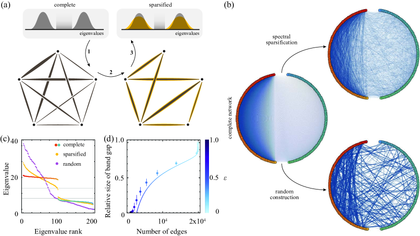
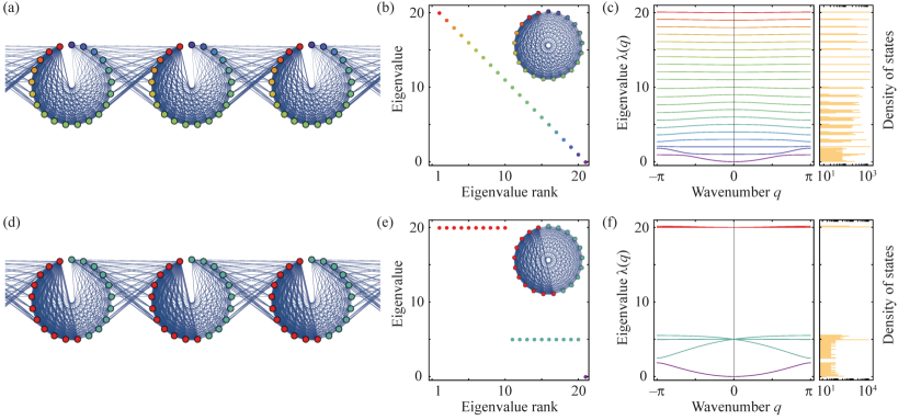
This construction allows us to create networks with precisely specified gaps. For instance, choosing and leads to a graph with edge weights if or and otherwise (Appendix A); that is, there are two groups of vertices, one strongly connected within itself and one weakly connected to everything. Adding a small amount of noise to each eigenvalue then lifts the eigenvalue degeneracy while preserving the connectivity structure and retaining a gap (Fig. 1b,c).
Since complete graphs can be difficult to realize physically, we explore the effect of the sparsification-by-resistances algorithm developed by Spielman and Srivastava [27]. Given an accuracy parameter , this sparsification creates a network with edges whose eigenvalues match the eigenvalues of the original network to within a multiplicative factor with high probability. Sparsification by resistances aims to preserve the entire spectrum, not just a gap; future sparsification algorithms directly constructed to preserve a gap could therefore improve on its efficiency. In other applications, the networks of interest are virtual ones [14] and sparsification may not be necessary.
We can use the multiplicative error bound to estimate the size of a discrete band gap after sparsification. Suppose we start from a network with eigenvalues , , and , with some multiplicities, where . The eigenvalues of the sparsified graph corresponding to should be no smaller than , while the eigenvalues corresponding to should be no larger than . The sparsified graph should therefore have a gap of size
| (4) |
That is, the gap contracts by a factor at most . For the parameters used in Fig. 1d, this is .
III Applications
We now demonstrate the practical potential of DBGs with three generic network models. In each case, we compare the dynamics on a complete DBG network (Fig. 1b, left) both to a sparsified approximate DBG network (Fig. 1b, top) and to a random connected network (Fig. 1b, bottom) constructed to have the same weighted vertex degrees as the DBG network (Appendix C). The gap is approximately preserved in the sparsified network and vanishes entirely in the random graph (Fig. 1c,d). Matching the degrees in the random graph to the DBG network ensures that any differences in dynamics are due to the gap and not differences in coarse features like the average connectivity. Often, the behavior of optimized networks is sensitive to small perturbations [40]; here, behaviors preserved in the sparsified graph are robust to significant changes.
Simulations were performed using a third or fourth order Adams-Bashforth linear multistep method with a time step . All simulations were written in C++ using Armadillo [41].
III.1 Kuramoto oscillators
Our first application is the Kuramoto model of coupled oscillators [42, 43]. Recent experiments coupling Belousov-Zhabotinsky reactions via a computer-controlled projector have shown the emergence of chimeras [14]; we will show this can be achieved in the Kuramoto model by designing an appropriately gapped spectrum. Here phases on the vertices evolve with a natural frequency and a nonlinear coupling defined by the network adjacency matrix:
| (5) |
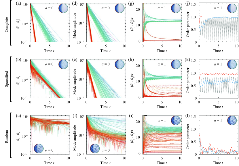
On any connected graph with , there is a single global attractor . The rate of convergence to this attractor is controlled by the eigenvalues of the Laplacian [15]. Both the complete and sparsified graphs have no eigenvalues near zero, so they synchronize much faster than the random graph (Fig. 2a-c). The gap divides the modes into two groups, one synchronizing faster than the other (Fig. 2d-e); moreover, on the complete graph, the localization of the eigenvectors causes staggered synchronization of vertices (Fig. 2a).
If is sufficiently large, the oscillators no longer synchronize at a single frequency. On DBG networks, global coherence gives way to weak chimera states [44] where vertices synchronize into two clusters with distinct frequencies (Fig. 2g-i, Movie 1). For the exactly-gapped network with edges of weight or there is a steady state with for and for . In this state,
| (6) |
The two phases and can synchronize if
| (7) |
This synchronization is possible if is small enough that the right hand side is less than one. If the two groups do not synchronize, and is not too large, the sine term in Eq. (7) will average to nearly zero giving an approximate mean frequency difference
| (8) |
which reduces to if as in Fig. 2. More general cluster synchronization [45, 46] could be achieved by adjusting the number and size of the gaps. In contrast, the random graph becomes thoroughly incoherent at comparable values of (Fig. 2i,l). The coherence can be quantified by the order parameter , which oscillates for the complete and sparsified networks but is near zero for the random graph (Fig. 2j-l), indicating complete disorder.
III.2 Swift-Hohenberg pattern formation
As the second application, we study generic Swift-Hohenberg pattern formation dynamics on a network [47, 48]. Consider a scalar field on the vertices obeying
| (9) |
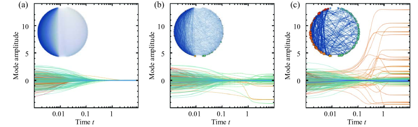
The fixed point , which exists for any values of the parameters , and , is linearly stable to perturbations in a Laplacian eigenmode with eigenvalue if the growth rate . With and positive, is negative for small and large , but choosing creates a range of unstable in between. This can drive pattern formation that is eventually stabilized by the nonlinearity. The patterns can only form, however, if has eigenvalues in the unstable range. Controlling the spectrum of therefore allows us to completely suppress pattern formation in arbitrarily large systems by placing a gap around the unstable region (Figs. 1c, 3a, Movie 2). If we sparsify the network with sufficiently small , the gap will be preserved and again no patterns will form. Eventually, though, increased sparsification will push some eigenvectors into the edges of the unstable region and bring back partial pattern formation (Fig. 3b), which becomes fully developed in the random graph (Fig. 3c). The maximum for which patterns will be fully suppressed for given parameter settings can be predicted straightforwardly from the expected changes in the eigenvalues, in a similar fashion to the post-sparsification gap size in Fig. 1d.
III.3 Gross-Pitaevskii localization
Having discussed two classical applications to non-conservative systems, we now show how DBGs can control quantum dynamics with conserved energy. In a network version of the Gross-Pitaevskii model [49, 50, 51], similar to those used in studying Bose-Einstein condensates in optical lattices [52], we find that the interplay of the total energy conservation constraint in such a model with the kinetic energy gap inhibits spreading of the wavefunction on DBG networks. Similarly to the Swift-Hohenberg example, we take the Gross-Pitaevskii equation for a complex wavefunction and replace the continuous Laplacian with its discrete analog :
| (10) |
This can be written , where the energy is the sum of the kinetic energy and the potential energy . The potential energy quantifies the localization of : with , it is large when the probability is concentrated at a single vertex and small when is spread out. Delocalization is limited by the size of the network, as , but can vary widely even on a finite network. If is initialized at a single vertex , then , independent of , while equals the degree of .
Since energy is conserved, the wavefunction can delocalize and reduce its potential energy only by converting it to kinetic energy. The rate of potential energy loss, set by , must therefore match the rate of kinetic energy gain, set by the differences in eigenvalues among the modes involved. Suppose the wavefunction is mostly in a localized mode with eigenvalue . Spreading to a higher mode with would increase kinetic energy by more than it would decrease potential energy, while a weak higher mode or a lower mode would not increase kinetic energy by enough, if at all. Both are barred by energy conservation. The amplitude in mode can only be reduced if there are other modes with .
To see this in more detail, suppose we have a wavefunction comprising two modes, , with initial complex amplitudes , . Suppose also that these eigenmodes are localized on two different vertices, with and . The system energy as a function of and is then
| (11) |
If the squared amplitudes change slightly, to and , the change in energy to leading order in is
| (12) |
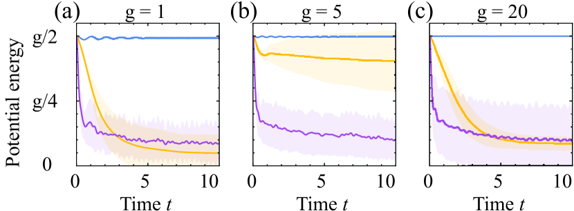
Conservation of energy requires , so in order to transfer a noticeable amplitude from the first mode to the second we must have . In the cases considered in Fig. 4, where and , this reduces to . Thus on a network with a spectral gap, the localization of can depend non-trivially on the interplay between and the spectrum.
Initializing at a weakly-connected vertex brings out this interplay as is varied (Movie 3). The initial state, with high potential energy and low kinetic energy, is localized on modes with eigenvalue below the spectral gap. On the sparsified network, a low value of makes nearby modes below the gap accessible for delocalization, causing the wavefunction to spread (Fig. 4a). However, increasing pushes the region where transfer is possible inside the spectral gap, inhibiting the spread of the wavefunction on the sparsified network (Fig. 4b). Further increase of once again enables delocalization as the modes above the gap becomes accessible for energy transfer (Fig. 4c). In contrast, the dense spectrum of the random graph means delocalization occurs in all three instances (Fig. 4). Interestingly, the complete DBG network appears to remain localized for all values of in our simulations (Fig. 4); this is likely due to the strong localization and near-zero overlap of the eigenmodes.
IV Band structure in periodic networks
We can construct infinite periodic networks in a standard way from any base network by tiling periodically and rewiring edges (Fig. 5a,d). Starting from the original vertex set for and edge weights , we make an infinite string of copies of with vertices indexed by , the label in , and , the unit cell. This will give a new, infinite Laplacian . For the edges that will not be rewired, we set for all . Doing this for all edges would leave the copies of disconnected. To connect them, we choose a subset of edges and rewire them to cross between unit cells; for example, if is an edge to be rewired to have in a unit cell to the left of we can set for all and symmetrically set . The remainder of the entries of are set to zero.
Since is periodic, Bloch’s Theorem allows us to write the eigenvectors as
| (13) |
where is a wavenumber in the first Brilloun zone . The then satisfy
| (14) |
which reduces to a new eigenvalue equation for a matrix of size :
| (15) |
where the matrix elements of are the same as those of for edges within a single unit cell and differ by a factor for edges that cross between unit cells and .
Using these transformations, which are standard in the study of lattice systems [17], we can find the continuous spectra of periodic tilings of our designed networks. Even without any optimization of which edges to rewire, the spectral characteristics persist in the infinite system. If we rewire all edges with , for example, a spectrum of equally-spaced eigenvalues leads to a density of states with corresponding equally-spaced large spikes (Fig. 5a-c), while a discrete band gap is almost entirely preserved (Fig. 5d-f). In both cases, only the bottom few bands vary significantly with . Note that, because we moved edges incident to the first vertex, all of the eigenvectors do change and are not localized for nonzero .
V Conclusions
Controlling dynamics on a network typically requires detailed understanding of its spectral properties. Here we have reversed the conventional approach by starting from a desired spectrum and providing a mathematically rigorous construction of a matching network. This enabled us to induce chimera states, suppress pattern formation, and control wavefunction localization [53] using suitably designed gapped spectra. Our method, which starts from global properties, complements traditional approaches using small-scale local rules to build and analyze networks [29, 54, 55, 56]. In the future, the above results may also prove useful as a standard of comparison for other networks. Contrasting the dynamics on an important class of networks with the dynamics on networks designed to have identical spectra can help identify the important features of that class. Moreover, as dynamics are often related to matrices other than the Laplacian [57], it will be interesting to investigate control of their spectra for weighted networks as well. Although our construction works optimally with fully-connected graphs, one can expect that improved sparsification algorithms together with recent progress in 3D printing and lithography [24, 18] may soon lead to physically-realizable networks with arbitrary gaps; since any graph can be embedded in 3D [58], the framework introduced here lays a conceptual foundation for the targeted design of complex non-periodic metamaterials with desired spectral properties. Currently, the approach can be applied directly to interfacing biochemical oscillators with computational networks [14]. Such hybrid networks can also be naturally extended to periodic systems, where the spectral properties are preserved well without any further optimization.
Acknowledgements. The authors would like to thank Jon Kelner and Philippe Rigollet for helpful discussions. This work was supported by Trinity College, Cambridge (F.G.W.), an Edmund F. Kelly Research Award (J.D.), and a Complex Systems Scholar Award of the James S. McDonnell Foundation (J.D.).
Appendix A Edge weights with a gap
Suppose we have eigenvalues with multiplicity and with multiplicity . Then if
| (16) |
Else, if and ,
| (17) |
There are two types of edges: edges with both endpoints in the first vertices have weight , while other edges have weight .
Appendix B Positivity of edge weights
The elements of the designed above the diagonal, for , are given by
| (18) |
From the second to third lines we use the definition of the eigenvectors in Eq. (1); the sum in the third line can be computed as a telescoping sum of partial fractions. is symmetric, so the elements below the diagonal must also be nonpositive. This proves that the edge weights of the constructed graph are nonnegative.
Appendix C Random equal-degree graphs
Given a weighted graph , we can construct a random simple graph with the same vertex degrees as as follows. Let denote the weight of edge and denote the weighted degree of vertex . Begin with a disconnected graph with a loop of weight at each vertex ; this has the same degrees as but is not simple. Repeat the following steps until there are no loops:
-
1.
Pick a loop and another edge at random, with .
-
2.
-
(a)
If , remove and add and with weight . Subtract from the weight of .
-
(b)
Else, remove and add and with weight . Subtract from the weight of .
-
(a)
Once there are no more loops, merge all sets of edges between the same pair of vertices into one edge with the same total weight. Since the degree of each vertex is preserved at each step, the final graph has the same degrees as . In the examples considered here, the algorithm terminates quickly.
References
- Hasan and Kane [2010] M. Z. Hasan and C. L. Kane, Rev. Mod. Phys. 82, 3045 (2010).
- Bradlyn et al. [2017] B. Bradlyn, L. Elcoro, J. Cano, M. G. Vergniory, Z. Wang, C. Felser, M. I. Aroyo, and B. A. Bernevig, Nature 547, 298 (2017).
- Sigmund and Jensen [2003] O. Sigmund and J. S. Jensen, Philos. Trans. R. Soc. A 361, 1001 (2003).
- Bardeen et al. [1957] J. Bardeen, L. N. Cooper, and J. R. Schrieffer, Phys. Rev. 108, 1175 (1957).
- Wang et al. [2017] P. Wang, Y. Zheng, M. C. Fernandes, Y. Sun, K. Xu, S. Sun, S. H. Kang, V. Tournat, and K. Bertoldi, Phys. Rev. Lett. 118, 084302 (2017).
- Souslov et al. [2017] A. Souslov, B. C. van Zuiden, D. Bartolo, and V. Vitelli, Nat. Phys. , doi:10.1038/nphys4193 (2017).
- Sonnenschein et al. [2013] B. Sonnenschein, M. A. Zaks, A. B. Neiman, and L. Schimansky-Geier, Eur. Phys. J.: Spec. Top. 222, 2517 (2013).
- Bianconi [2015] G. Bianconi, EPL 111, 56001 (2015).
- Ronellenfitsch and Katifori [2016] H. Ronellenfitsch and E. Katifori, Phys. Rev. Lett. 117, 138301 (2016).
- Tayar et al. [2015] A. M. Tayar, E. Karzbrun, V. Noireaux, and R. H. Bar-Ziv, Nat. Phys. 11, 1037 (2015).
- Brockmann et al. [2006] D. Brockmann, L. Hufnagel, and T. Geisel, Nature 439, 462 (2006).
- Cohen and Horowitz [1991] J. E. Cohen and P. Horowitz, Nature 352, 699 (1991).
- Yook et al. [2002] S.-H. Yook, H. Jeong, and A.-L. Barabási, Proc. Natl. Acad. Sci. U.S.A. 99, 13382 (2002).
- Totz et al. [2017] J. F. Totz, J. Rode, M. R. Tinsley, K. Showalter, and H. Engel, Nat. Phys. (2017), 10.1038/s41567-017-0005-8.
- McGraw and Menzinger [2008] P. N. McGraw and M. Menzinger, Phys. Rev. E 77, 031102 (2008).
- Nakao and Mikhailov [2010] H. Nakao and A. S. Mikhailov, Nat. Phys. 6, 544 (2010).
- Lubensky et al. [2015] T. C. Lubensky, C. L. Kane, X. Mao, A. Souslov, and K. Sun, Rep. Prog. Phys. 073901, 73901 (2015).
- Man et al. [2013] W. Man, M. Florescu, K. Matsuyama, P. Yadak, G. Nahal, S. Hashemizad, E. Williamson, P. Steinhardt, S. Torquato, and P. Chaikin, Opt. Express 21, 19972 (2013).
- Han et al. [2007] M. Y. Han, B. Özyilmaz, Y. Zhang, and P. Kim, Phys. Rev. Lett. 98, 206805 (2007).
- Gladman et al. [2016] A. S. Gladman, E. A. Matsumoto, R. G. Nuzzo, L. Mahadevan, and J. A. Lewis, Nat. Mater. 15, 413 (2016).
- Wang et al. [2015] K. Wang, Y.-H. Chang, Y. Chen, C. Zhang, and B. Wang, Mater. Des. 67, 159 (2015).
- Bhattacharjee et al. [2016] N. Bhattacharjee, A. Urrios, S. Kang, and A. Folch, Lab Chip 16, 1720 (2016).
- Huang et al. [2017] L. Huang, R. Jiang, J. Wu, J. Song, H. Bai, B. Li, Q. Zhao, and T. Xie, Adv. Mater. 29, 1605390 (2017).
- Bückmann et al. [2012] T. Bückmann, N. Stenger, M. Kadic, J. Kaschke, A. Frölich, T. Kennerknecht, C. Eberl, M. Thiel, and M. Wegener, Adv. Mater. 24, 2710 (2012).
- Motter [2015] A. E. Motter, Chaos 25, 097621 (2015).
- Martens et al. [2013] E. A. Martens, S. Thutupalli, A. Fourriére, and O. Hallatschek, Proc. Natl. Acad. Sci. U.S.A. 110, 10563 (2013).
- Spielman and Srivastava [2008] D. A. Spielman and N. Srivastava, SIAM J. Comp. 40, 1913 (2008).
- Kelner and Levin [2013] J. A. Kelner and A. Levin, Theory Comp. Syst. 53, 243 (2013).
- Barabasi and Albert [1999] A.-L. Barabasi and R. Albert, Science 286, 509 (1999).
- Arenas et al. [2006] A. Arenas, A. Díaz-Guilera, and C. J. Pérez-Vicente, Phys. Rev. Lett. 96, 114102 (2006).
- Peixoto [2013] T. P. Peixoto, Phys. Rev. Lett. 111, 098701 (2013).
- Amir et al. [2010] A. Amir, Y. Oreg, and Y. Imry, Phys. Rev. Lett. 105, 070601 (2010).
- Ipsen and Mikhailov [2002] M. Ipsen and A. S. Mikhailov, Phys. Rev. E 66, 6 (2002).
- Comellas and Diaz-Lopez [2008] F. Comellas and J. Diaz-Lopez, Physica A 387, 6436 (2008).
- Cvetkovič [2012] D. Cvetkovič, Yugoslav J. Oper. Res. 22, 145 (2012).
- McKay [1977] B. D. McKay, Ars Comb. 3, 219 (1977).
- Halbeisen and Hungerbühler [2000] L. Halbeisen and N. Hungerbühler, Eur. J. Comb. 21, 641 (2000).
- Van Dam and Haemers [2003] E. R. Van Dam and W. H. Haemers, Linear Algebr. Appl. 373, 241 (2003).
- Pradhan et al. [2017] P. Pradhan, A. Yadav, S. K. Dwivedi, and S. Jalan, Phys. Rev. E 96, 022312 (2017).
- Nishikawa et al. [2017] T. Nishikawa, J. Sun, and A. E. Motter, Phys. Rev. X 041044, 1 (2017).
- Sanderson and Curtin [2016] C. Sanderson and R. Curtin, J. Open Source Software 1, 26 (2016).
- Kuramoto [1975] Y. Kuramoto, Int. Symp. Math. Prob. Theor. Phys. 39, 420 (1975).
- Strogatz [2000] S. H. Strogatz, Phys. D 143, 1 (2000).
- Ashwin and Burylko [2015] P. Ashwin and O. Burylko, Chaos 25, 013106 (2015).
- Cho et al. [2017] Y. S. Cho, T. Nishikawa, and A. E. Motter, Phys. Rev. Lett. 119, 1 (2017).
- Pecora et al. [2014] L. M. Pecora, F. Sorrentino, A. M. Hagerstrom, T. E. Murphy, and R. Roy, Nat. Comm. 5, 4079 (2014).
- Swift and Hohenberg [1977] J. Swift and P. C. Hohenberg, Phys. Rev. A 15, 319 (1977).
- Nicolaides et al. [2016] C. Nicolaides, R. Juanes, and L. Cueto-Felgueroso, Sci. Rep. 6, 21360 (2016).
- Brunelli et al. [2004] I. Brunelli, G. Giusiano, F. P. Mancini, P. Sodano, and A. Trombettoni, J. Phys. B 37 (2004).
- Bang et al. [1994] O. Bang, J. J. Rasmussen, and P. L. Christiansen, Nonlinearity 7, 205 (1994).
- Pelinovsky et al. [2014] D. E. Pelinovsky, D. A. Zezyulin, and V. V. Konotop, J. Phys. A 47 (2014).
- Greiner et al. [2002] M. Greiner, O. Mandel, T. Esslinger, T. W. Hansch, and I. Bloch, Nature 415, 39 (2002).
- Amir et al. [2013] A. Amir, J. J. Krich, V. Vitelli, Y. Oreg, and Y. Imry, Phys. Rev. X 3, 021107 (2013).
- Bianconi and Barabási [2000] G. Bianconi and A. Barabási, Europhys. Lett. 54, 436 (2000).
- Lorimer et al. [2015] T. Lorimer, F. Gomez, and R. Stoop, Sci. Rep. 5, 12353 (2015).
- Milo et al. [2002] R. Milo, S. Shen-Orr, S. Itzkovitz, N. Kashtan, D. Chklovskii, and U. Alon, Science 298, 824 (2002).
- Yan et al. [2015] G. Yan, G. Tsekenis, B. Barzel, J.-J. Slotine, Y.-Y. Liu, and A.-L. Barabási, Nat. Phys. 11, 779 (2015).
- Cohen et al. [1997] R. F. Cohen, P. Eades, T. Lin, and F. Ruskey, Algorithmica 17, 199 (1997).