Robust PCA for Anomaly Detection in Cyber Networks

Abstract

This paper uses network packet capture data to demonstrate how Robust Principal Component Analysis (RPCA) can be used in a new way to detect anomalies which serve as cyber-network attack indicators. The approach requires only a few parameters to be learned using partitioned training data and shows promise of ameliorating the need for an exhaustive set of examples of different types of network attacks. For Lincoln Lab’s DARPA intrusion detection data set, the method achieves low false-positive rates while maintaining reasonable true-positive rates on individual packets. In addition, the method correctly detected packet streams in which an attack which was not previously encountered, or trained on, appears.

Keywords: robust principal component analysis, anomaly detection, computer networks, cyber defense

I Introduction

Over the past decades the dependence of society on interconnected networks of computers has exponentially increased, with many sectors of the world economy, such as banking, transportation, and energy, being dependent on network stability and security. Accordingly, maintaining the integrity of computer networks is imperative, and much research has been performed in this challenging problem domain [18, 23, 17, 19, 20]. In this paper we focus on a sub-topic in this important domain, namely that of anomaly detection.

Highlights of our results include:

• We have developed a novel robust principal component approach for anomaly detection. Instead of classic methods where nominal background activity (which is presumed to lay on a low-dimensional subspace) is defined using some a priori threshold, we instead optimize our thresholds for the current network of interest and assume noisy and missing data.

• As the vast majority of our parameters are trained in an unsupervised fashion (i.e., requiring no labeled data), and we only have two parameters trained on labeled data, we can make efficient use of the limited labeled data available in many real world cyber-anomaly detection problems.

• We demonstrate our performance on three scenarios from the DARPA Lincoln Lab Intrusion Detection Evaluation Data Set (https://www.ll.mit.edu/ideval/data/2000/LLS_DDOS_1.0.html). The attack scenarios are shown in Table I. We trained on the first two scenarios and then, on the third, we achieve close to zero false positive rates while maintaining reasonable true positive rates even though our algorithm was provided no training information for that attack.

Scenario 1	IP sweep from a remote site
Scenario 2	A probe of live IP addresses looking for a running Sadmind daemon
Scenario 3	An exploitation of a Sadmind vulnerability

TABLE I: The attack scenarios in the DARPA Lincoln Lab Intrusion Detection Evaluation Data Set on which we test our detection algorithms.

I-A Background

Of course, before any progress can be made in the detection of anomalies, one must carefully consider how such anomalies may be defined. In particular, for the automated detection of such anomalies to be useful for detecting attacks in real-world cyber-data one must consider their definition both from the computer network perspective and the mathematical perspective.

An anomaly in a computer network can take many forms. They include:

• extreme anomalies, such as a distributed denial of service attack (DDoS),

• moderate anomalies, such as port scans, and

• subtle anomalies, such as a buffer overflow attack.

However, for an anomaly to be detectable it must be the case that it is different in some way from the normal operations of the network. For example, if an intrusion detection system (IDS) is installed on the network, and it performs port scans to detect when users have inappropriately opened ports, then a port scan is not prima faci an anomaly for that network. One could now imagine making a long list of rules or templates, such as “port scans are anomalies, unless they originate from a specified address”, and this is precisely how some IDS systems operate. However, we are focused on the difficult problem of detecting anomalies where no template for the anomaly is known. Accordingly, rather than enumerating possible anomalies, we focus on understanding the normal operating modes of a computer network, and define as anomalous any departure from this normal operating mode.

Accordingly, our goal is to extend the body of literature which aims to detect anomalies by way of low-dimensional representations of data measured from computer networks [2, 24, 16, 17, 20]. For real-world cyber-data, such as network packet captures (PCAP), it has been observed that the resulting data often, under normal conditions, resides on a low-dimensional subspace of the ambient, or measurement, space. A classic approach to anomaly detection is to compute the low-dimensional subspace on which the nominal PCAP data resides and then detect packets that do not lay on this low-dimensional subspace [17, 7, 29, 25]. Such packets can be marked as anomalous.

Note, raw packets extracted from PCAP files can sometimes be difficult to process. For example, if the packet payloads are compressed or encrypted, then the dimension of the subspace on which the packets reside can be unnecessarily large. Accordingly, in our work we pre-process the packets to extract features such as port numbers, IP addresses, packet size, etc. We have even added additional derived features, such as whether a packet originated within the network or is from outside. As we will demonstrate, representing packets using such features gives rise to low-dimensional subspaces and leads to good detection performance.

A classic approach to computing a low-dimensional subspace which approximates a collection of data is Principal Component Analysis (PCA) [13, 15]. Given a collection of points, PCA computes a linear projection of the points to a low-dimensional subspace that minimizes the $\ell_{2}$ error between the original points and the projected points.

PCA is a workhorse of many data analysis domains including machine learning and data visualization [15, 27, 3]. However, it is well known that the low dimensional subspace provided by PCA is sensitive to outliers.

In particular, outliers will tend to pull the subspace toward the outlier quadratically, making the distance undesirably small between the computed subspace and the outliers one wishes to detect. More precisely, PCA computes a family of low-dimensional subspaces, and the user is required to select which $k$-dimensional subspace they believe is the best representation of the data. However, this selection is made difficult when each subspace is computed from a mixture of nominal and anomalous measurements. As our aim is anomaly detection in real-world network data, a more delicate analysis is likely required.

I-B Potential of RPCA

Accordingly, herein our focus is on the growing field of robust principal component analysis (RPCA). RPCA has a large and active extent literature [11, 12, 10, 23, 22, 28], and there are many algorithms that focus on the recovery of low-dimensional subspaces from data which has been corrupted by outliers.

In particular, much work has been performed on recovery problems where theorems are proved, and numerical demonstrations provided, along the lines of:

Assuming there exists a true low dimensional subspace $L$ and a true collection of anomalies $S$, one recovers approximations of these values from their sum $M=L+S$ (or some other similar combination of $L$ and $S$) assuming $L$ and $S$ satisfy some conditions [10, 28].

Such problems are quite non-trivial and have received much attention [10, 28]. In particular, since many combinations of $L$ and $S$ give rise to the same $M$, recovering a specific desired pair $L,S$ purely from such an $M$ often requires delicate analysis.

However, as opposed to such recovery problems, herein we take a novel approach and instead concern ourselves with detection problems. Hearkening back to the case of classic PCA, one can ask two quite different questions:

1. Given some data (perhaps corrupted by noise) can one recover the true low dimensional subspace that spans the data (with the corruptions removed)?

2. Given some data can one find a low dimensional subspace that is most effective for some other downstream detection algorithm. I.e., how is PCA best used as a preprocessing step for some other machine learning algorithm?

Both approaches are used quite widely in the PCA literature [25] and it is questions similar to the second question above that inspire our approach here. For example, when using PCA as a preprocessing step for some downstream algorithm, it is quite classic to consider either a target dimension $k$ for the computed subspace or, equivalently, a desired threshold $\gamma$ for the singular values of a low-rank data matrix $L$. Such a threshold is equivalent to a statement about the maximum acceptable error between the original data points and their projection.

Accordingly, $\gamma$ can either be chosen based upon some a priori target error tolerance in the singular values or, as we propose here, chosen based upon the cross validated detection performance of the detection algorithm. Similarly, one can ask two different questions of RPCA. As we will discuss in detail in the sequel, the RPCA algorithms that we leverage herein have a parameter $\lambda$ which controls the trade-off between the low-rank matrix $L$ and the sparse matrix $S$. Mirroring the idea in the PCA case, we ask the following question:

1. Given some data (perhaps corrupted by noise), how should one $\lambda$ that best leads to the recovery of the true low-dimensional subspace and the true sparse anomalies from which the observed data was constructed?

2. Given some data, how should one find a dimension $k$ and a value of $\lambda$ that lead to a low-dimensional subspace and a set of anomalies that is most effective for some other downstream detection algorithm that only gets to train $\lambda$ and not the numerous other parameters of the algorithm? I.e., how is RPCA best used as a preprocessing step for some other machine learning algorithm?

In one of the key novelties of our analysis, we demonstrate that a cross validated choice of $\lambda$ rather than choosing $\lambda$ based upon some recovery principle, can lead to substantially improved algorithms for detecting anomalies in computer networks. In particular, there are no current approaches that use RPCA for detecting anomalies in computer networks, of which we are aware, that avail themselves of the full flexibility of RPCA. In particular, they do not select the key parameter $\lambda$ based upon a cross validation principle.

In particular, herein we demonstrate the efficacy of our approach on PCAP measurements from the Lincoln Labs DARPA Intrusion Detection Data Set (https://www.ll.mit.edu/ideval/data/2000/LLS_DDOS_1.0.html), which cover a swath of normal computer network operations and a variety of different attack scenarios. Perhaps most interestingly, using our methods we are able to train our parameters such as $\lambda$ on a small set of attacks, but then we are able to use these same parameter settings to detect different attack modalities on which the algorithm was not trained.

In Section II we describe the mathematical foundation of our approach, in Section III we describe the setup of our experiments and the data set we use for validation, in Section IV we demonstrate our results, and in Section V we provide a summary and pointers to future work. Finally, in the Appendix we provide additional notes on the effecient solution of the problems of interest using the Augmented Lagrangian Method and the Alternating Direction Method of Multipliers.

I-C Contribution and previous work

PCA is a standard algorithm in many problem domains [15] and it has been widely applied in computer network analysis [7] (and reference therein) with seminal work going back to at least 2004 [18]. In addition, there are several examples of RPCA being used in the extant literature for computer network anomaly detection [2, 24, 16, 17, 20] (and references therein) with a quite recent review to be found in the 2015 Ph.D. thesis [21] and related paper [20]. However, only the more recent references [24, 2, 20] use the modern convex nuclear norm approaches we leverage here.

In particular, [2] uses a RPCA on data which is similar to our own, but they take the opposite approach to ours when considering the coupling constant $\lambda$. They use the theoretical value suggested in [10] and do not study the interplay between $\lambda$ and the performance of the downstream detection algorithms.

Accordingly, a key novelty of our approach is a careful treatment of the parameter $\lambda$ which is the key element in balancing the importance of low-dimensional $L$ and the anomalous $S$. In particular, by studying the interplay between $\lambda$ and downstream detection algorithms, the quality of our detection results are greatly enhanced as compared to PCA. In addition, we analyze a detection threshold on the anomalies $S$, here denoted by $\alpha$, which in our experiments turns out to essentially be $1$ given a judicious choice of $\lambda$.

II Approach

II-A PCA

We begin the derivation of our methodology by considering a collection of points $\{y_{0},...,y_{n}\}$ with $y_{i}\in\mathbb{R}^{m}$. Each point can be thought of a collection of features that represent a measurement of our computer network. For example, as we will detail in Section III, herein we view each $y_{i}$ as a collection of features derived from a single Internet packet (such as IP address, port number, etc.). Therefore, the collection of points $\{y_{0},...,y_{n}\}$ represents some collection of packets measured across different computers and times. Given such a collection of points $\{y_{0},...,y_{n}\}$, the goal of PCA is to compute a linear projection of the points $\{\hat{y}_{0},...,\hat{y}_{n}\}$ with each of the $\hat{y}_{i}$ laying on a specified $k$-dimensional subspace of $\mathbb{R}^{n}$.

To specify the desired $k$-dimensional subspace of $\mathbb{R}^{n}$ one can encode the original points $y_{i}$ into a data matrix $[y_{0},...,y_{n}]=Y\in\mathbb{R}^{m\times n}$ (i.e., by having each $y_{i}$ be a column of $Y$). One can then compute the desired $k$-dimensional subspace by solving the optimization problem

$$\min_{L}\|L-Y\|_{F}^{2}$$ (1)

subject to $$\rho(L)\leq k$$

where $L\in\mathbb{R}^{m\times n}$, $\|L-Y\|_{F}^{2}$ is the Frobenius norm of $L-Y$ (i.e., the sum of the squares of the entries of $L-Y$), and $\rho(L)$ is the rank of $L$ (i.e., $\rho(L)$ is the number of non-zero singular values of the matrix $L$).

A more common derivation of PCA is in terms of the Singular Value Decomposition (SVD) [13] rather than as an optimization as in (1). However, the optimization point of view will have an important role to play in the sequel.

In particular, given a matrix $Y\in\mathbb{R}^{m\times n}$, one can always write

$$Y=U\Sigma V^{T}$$ (2)

where $U\in\mathbb{R}^{m\times m}$ and $V\in\mathbb{R}^{n\times n}$ are unitary (i.e., $UU^{T}=I$ and $VV^{T}=I)$, and $\Sigma$ is diagonal. In addition, the diagonal entries of $\Sigma$, denoted $\Sigma_{ii}=\sigma_{i}$ are called the singular values of $Y$.

In a seminal result, Eckart and Young in their 1936 paper [13] proved that the optimization problem in (1) can be solved in closed from by setting

$$L=U\hat{\Sigma}V^{T}$$ (3)

where $\hat{\Sigma}$ is computed from $\Sigma$ by setting the $m-k$ smallest singular values $\sigma_{i}$ to $0$ (i.e., by retaining only the $k$ largest singular values), and $L$ is therefore a low-rank approximation of $Y$. Similarly, one can compute a projection of $Y$ onto the coordinate system of the $k$-dimensional subspace by using the formula

$$X=\hat{\Sigma}V^{T}$$ (4)

and removing the zero rows of $X$ arising from the $0$ values on the diagonal of $\hat{\Sigma}$. An example of PCA is shown in Figure 1. Note, the relationship between the optimization view of PCA, as shown in (1), and the linear algebra view, as exemplified by the SVD, will be important in the sequel. In particular, while the SVD is the most common implementation of PCA in current use, it is actually the optimization version that inspires much recent work. In particular, there are many recent results in robust versions of PCA methods which revolve around hearkening back to the optimization roots of PCA.

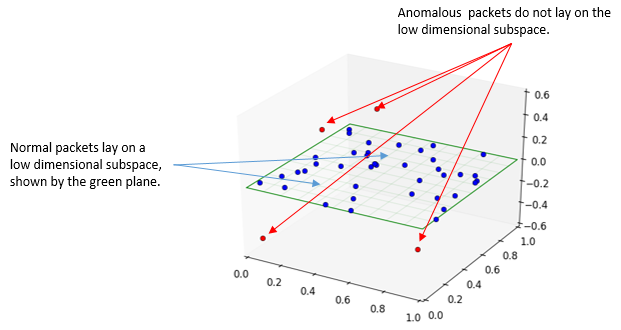
Figure 1: In this figure we show an example of the key idea of anomaly detection by way of PCA. Nominal data is assumed to lay on a low-dimensional linear subspace and anomalies are defined as any departures from this low-dimensional subspace.

II-B RPCA

PCA, while a widely used technique for dimensionality reduction, is unfortunately sensitive to the presence of outliers. In particular, as shown in Figure 2, even when the vast majority of the measurements in $Y$ lay on a low-dimension subspace, the presence of just a few outliers can substantially increase the dimension of the subspace produced by the PCA algorithm and lead to a reduction in our ability to later detect anomalies. Note, this is not an issue that can be fixed by merely a judicious choice of $k$. Every singular value produced by (1) can, and likely would be, perturbed by even a single outlier. In particular, outliers can easily transform singular values which, for purely nominal data, would be close to $0$ to arbitrarily large values, and thereby increase the detected dimension.

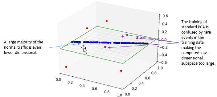
Figure 2: In this figure we show an example of the key idea of the RPCA algorithm. The nominal data is corrupted by rare events (either anomalous or not) and this data makes the computed dimension too large. The truly nominal data is lower dimensional than PCA reveals. I.e., even with a large threshold for the singular values, PCA would conclude that the data is two-dimensional. RPCA detects these events and provides a better representation of the low-dimensional state of the network.

Fortunately, there has been a flurry of recent attention paid to Robust Principal Component Analysis (RPCA) and excellent progress has been made in the literature. We provide a very brief overview of the main ideas, and refer the reader to [11, 10, 12, 8] for more details. In this section we closely follow the notation and derivation from [23, 22]

As noted in [10], the RPCA problem may seem daunting upon preliminary inspection. Given a measurement matrix $Y$, we must tease apart a low rank matrix $L$ and a set of sparse anomalies $S$ without knowing a priori the true dimension $k$ of $L$, nor knowing the number or locations of the anomalous entries in $S$. Similar to (1), this problem can be phrased as an optimization problem by writing

$$\min_{L,S}\rho(L)+\lambda\|S\|_{0}$$ (5)

subject to $$|Y-(L+S)|=0$$

where $\rho(L)$ is the rank of $L$, $\|S\|_{0}$ is the number of non-zero entries in $S$, and $\lambda$ is a coupling constant which controls the trade-off between the low-rank matrix $L$ and the sparse matrix $S$. Unfortunately, as opposed to (1), we do not have any closed form solution to (5). Even worse, a näive, brute force approach to the problem, where one searches over all possible combinations of low-rank matrices $L$ and entries of $S$ corresponding to a presupposed number of anomalies, would be NP-hard in the number of anomalies.

However, Theorem 1.2 in [10], Theorem 2.1 [23], and many similar theorems in the extent literature provide remarkable guarantees for recovery $L$ and $S$. Providing details for these theorems would take us too far afield in the current context, and the interested reader may refer to extent literature for details [11, 9, 12, 10, 23, 22]. Herein we merely observe that the optimization in (5) is NP-hard, but a closely related problem can be solved if some technical conditions are met.

In particular, assuming such conditions are met, then, with high probability the convex program

$$\min_{L,S}\|L\|_{*}+\lambda\|S\|_{1}$$ (6)

subject to $$|Y-(L+S)|\preceq\epsilon$$

recovers $L$ and $S$, where $\|L\|_{*}=\sum_{i=1}^{m}\sigma_{i}$ is the nuclear norm of $L$ (i.e., the sum of the singular values of $L$) and $\|S\|_{1}:=\sum_{ij}|S_{ij}|$. $\lambda$ is as in (5) and $\epsilon$ is a set of point-wise error constraints which we used to ameliorate the noise found in real-world data. The reader familiar with such algorithms will no-doubt note that $\|S\|_{1}$ is a convex relaxation of $\|S\|_{0}$, and $\|L\|_{*}$ is a convex relaxation of $\rho(L)$, and such problems can be efficiently solved [6, 11, 10, 23, 22, 14].

Note, in (6), the importance of the parameters $\lambda$ and $\epsilon$. In particular, Theorem 1.2 in [10] proves that setting $\lambda=\frac{1}{\sqrt{\max(m,n)}}$, where $Y\in\mathbb{R}^{m\times n}$ guarantees the recovery of $L$ and $S$ from $Y$ (assuming the constraints mentioned previously).

However, in the current context, the recovery of a presumed $L$ and $S$ is not our goal. In particular, as we are attempting to detect anomalies in real-world measured data, it is not clear what such a “true” $L$ and $S$ would mean, even if we were to compute them. Accordingly, in our work, we view $\lambda$ and $\epsilon$ as parameters to be estimated from training data, and tuned to our particular detection task. Of course, having $\lambda$ and $\epsilon$ as parameters we learn from data requires us to be in possession of appropriate training data. However, as we will demonstrate in Section IV, it is our view that the additional requirements for training data are well worth the substantially better performance we achieve.

As a foreshadowing of those results, see Figure 3. There we show the singular values of $L$ computed from a collection of PCAP features encoded in a measurement matrix $Y$ (which we will detail in the next section). Observe how various choices of $\lambda$ have a profound effect on the dimension of the computed low-rank matrix $L$. As one might imagine, the ability to choose an appropriate value of $\lambda$, and therefore an appropriate low-rank $L$, has an equally profound effect on the ability of the algorithm to detect anomalies.

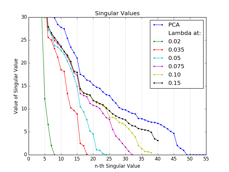
Figure 3: This figure shows the number of non-zero singular values of various low-rank matrices $L$ computed from the same measurement matrix $Y$. These $L$-matrices are calculated with values of $\lambda$ ranging from 0.02 through 0.15, whose lines are labeled as such. The PCA line is equivalent to sending $\lambda$ to infinity. As $\lambda$ increases, the number of non-zero singular values increases to our maximum allowed rank (40). $\lambda=0.15$ has 40 non-zero singular values (and does not reach our iteration threshold (1000)). The SVD of $Y$ has 94 singular values but the latter 55 are the same. In calculation, we will be treating this as 49 non-zero singular values. As for $\lambda=$ 0.02, 0.035, 0.05, 0.075, and 0.10, we have 8, 18, 24, 32, and 38 non-zero singular values, respectively. Larger values of $\lambda$ makes placing anomalies into $S$ more expensive, and generally increase the rank. On the other hand, smaller values of $\lambda$ makes placing anomalies into $S$ less expensive. Interestingly, the relation between $\lambda$ and the number of non-zero singular values is not necessarily linear.

III Problem setup and feature selection

III-A Problem setup

To demonstrate the effectiveness of our proposed techniques we make use of PCAP measurements from the Lincoln Labs DARPA Intrusion Detection Data Set (https://www.ll.mit.edu/ideval/data/2000/LLS_DDOS_1.0.html). This data set cover a swath of normal computer network operations and a variety of different attack scenarios including

• IP sweeps,

• probing and breaking in through the Sadmind daemon, and

• the preparation and execution of a Distributed Denial of Service (DDoS) attack.

We chose to use the PCAP data in our experiments since it represents the most fundamental measurement for network problems. However, in future work, there are many other paths that we could consider, such as stream based measurements.

As a preprocessing step we leveraged Wireshark [5, 4, 26] to convert the original PCAP files into comma separated value (CSV) files, and we then performed the bulk of the processing using the Python [1] scripting language. The raw CSV files from Wireshark include the following features directly extracted from the PCAP files: Source IP address, Destination IP address, Source Port, Destination Port, Protocol, packet length, and the packet time.

From this raw PCAP data we have chosen to create a number of higher level features derived from this base feature set. Perhaps most importantly, we one-hot encode [15] our non-numerical values, such as IP addresses, to create numerical values appropriate for analysis. For example, for each unique IP address that appears as a source IP address in a packet header, we create a row of $Y$ which is $1$ if that packet in from that IP address, and is $0$ otherwise. Similarly, while a port number is an integer, port numbers do not have the same semantics as integers (e.g., port numbers 79, the Finger protocol, and 80, the HTTP protocol, are not really that close to each other in functionality). Accordingly, we have rows of $Y$ corresponding to several ports that we consider to be important, encoded using the same $0$ or $1$ scheme.

In summary, our higher level features are shown in Table II

27 0-1 features	unique source IP addresses
27 0-1 features	unique destination IP addresses
13 0-1 features	important system ports on the source side
13 0-1 features	important system ports on the destination side
2 0-1 features	distinguish ports below 1024 from those above 1024 on the source side
2 0-1 features	distinguish ports below 1024 from those above 1024 on the destination side
1 0-1 feature	designate missing port number on the source side
1 0-1 feature	designate missing port number on the destination side
7 0-1 feature	various protocols (ICMP, sadmind, Portmap, TELNET, TCP, FTP, and HTTP)
1 numerical feature	number of bytes in the packet

TABLE II: The features that we derive from PCAP data.

This gives a $Y$ matrix with a total of 94 rows, 54 for IP addresses, 32 for ports, 7 for protocols, and 1 for packet length.

With the above features in mind, we extract from the full Lincoln Lab dataset a subset comprised of $8322$ packets. We then have a data matrix $Y\in\mathbb{R}^{m\times n}$ where $m=94$ and $n=8322$. In particular, as shown in Figure 4, our data can be viewed as a set of three attack stages, with a large region of nominal data proceeding the first attack stage, and smaller regions of nominal data between each of the following attack stages. The attack stages are shown in Table I. However, it is important to emphasize that even the areas of the data where the attacks are occurring, the attack packets are quite sparse and interspersed/masked by a substantial percentage of normal data. A cartoon of the set-up of $Y$ can be found in Figure 4.

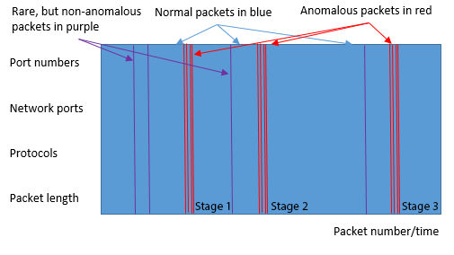
Figure 4: This figure shows our experimental setup. Nominal packets (shown in blue) are interspersed with nominal, but rare, events (shown in purple) and the three attack scenarios, from Table I (shown in red).

III-B Decision algorithm

With the details from Sections III-A in mind, we can now precisely state our method for detecting anomalies in the Lincoln Labs DARPA Intrusion Detection Data Set. The training of our algorithm can be best explained by referring to Figure 4. In particular, we take the data before the stage one attack in Figure 4 and denote it by $Y_{0}$. We then use $Y_{0}$ to compute a nominal $L_{0}$ and $S_{0}$ using (5) and (6). In particular, there are rare, but not anomalous events even before the stage one attack that appear in $Y_{0}$. Accordingly, the $S_{0}$ matrix is certainly not empty, even before the first attack occurs. The nominal $L_{0}$ matrix is, we believe, a more accurate representation of the true nominal processing of the network.

In effect, our goal is to identify points which are at distance greater than a threshold $\alpha$ from the subspace spanned by $L_{0}$ (where distance is measured using the $\|\cdot\|_{\infty}$ norm). Accordingly, given a training $Y_{0}$ as constructed in Section III-A, and appropriate parameters $\lambda$ and $\alpha$ (whose selection we will detail in Section III-C), we can run the RPCA procedure in (6) to produce a nominal $S_{0}$ and $L_{0}$. We then extract a data matrix $Y_{a}$ that overlaps one of the attack stages, but does not necessarily overlap $Y_{0}$, and project $Y_{a}$ onto the subspace spanned by $L_{0}$ to compute $L_{a}$. This can be thought of as extracting the nominal part of $Y_{a}$. We can compute the anomalies for $Y_{a}$ by simply setting $S_{a}=Y_{a}-L_{a}$. With $S_{a}$ in hand, our detection scheme is quite simple. We will merely flag as anomalous any columns in $S_{a}$ (which is equivalent to flagging a particular packet), whose maximum entry is larger than some threshold $\alpha$. In other words, we flag as anomalous any packet whose corresponding column of $S_{i}\in S$ has $\|S_{i}\|_{\infty}=\max_{j}|S_{ij}|>\alpha$.

III-C $\lambda$ and $\alpha$ training

The selection of our values for $\lambda$ and $\alpha$ can again be best explained by referring to Figure 4. In particular, as before, we chose to compute our nominal $L_{0}$ and $S_{0}$ on $Y_{0}$.

Using our notation from Section II, our first stage of training is to compute a sequence of $L_{0}$ and $S_{0}$ matrices as we vary $\lambda$, with small $\lambda$ values leading to lower dimensional $L_{0}$ matrices and higher values of $\lambda$ leading to higher dimensional $L_{0}$ matrices. We then select the value of $\lambda$ that leads to the best detection performance on the stage one and stage two attacks. However, the $\lambda$ value we use does not use any training data from the stage three attacks. We then chose $\alpha$ by fixing $\lambda$ (and thereby fixing $L_{0}$ and $S_{0}$) and selecting which $\alpha$ value gives the best detection performance over the same two stages, again not using any data from the quite different stage three attack. The stage three attack remains pristine, allowing for a true cross validation experiment which would be similar to how the algorithm would be used in the field.

IV Numerical Results

In this section we show a variety of results arising from our analysis. In particular, we demonstrate that a RPCA method, with a $\lambda$ value optimized for attack detection can provide superior results to both a standard PCA analysis and a RPCA analysis that uses a $\lambda$ value based upon some matrix recovery principal.

We begin with Figure 5, where we show a standard PCA analysis. As can be seen, the PCA analysis misses the vast majority of attack packets in all three attack stages. PCA is able to detect a few attack packets, but only at the cost of numerous false negatives. We conjecture, as demonstrated in Figure 3, that the dimension of the subspace generated by PCA is too large, and therefore many packets which are in fact anomalous actually end up laying close to the normal subspace $L$ generated by the training data $Y_{0}$. It is important to note that, as already discussed in Section II-A, that the dimension $k$ in the standard PCA algorithm can be selected to make the dimension of $L$ arbitrarily large or small. However, by the very nature of the optimization (1), the PCA algorithm forces the detected anomalies to be small numbers, and thereby substantially complicates the decision algorithm in Section III-B. It is an interesting path for future research to compare decision algorithms customized to different dimension reduction procedures.

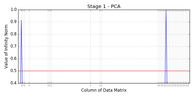
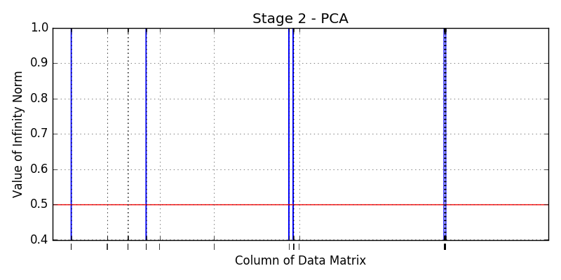
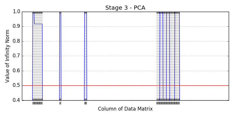
Figure 5: Here we show detection results for our three attack stages and detected using a PCA based algorithm for generating a low-dimensional subspace from our training data $Y_{0}$ and the detection scheme discussed in Section III-B. The red lines represent the detection threshold, the blue lines show the detected anomalies (which raise an alarm when the blue line is above the red detection threshold), and black dotted lines which mark the true attacks. As you can see, the PCA algorithm misses most of the attacks in stage one and two, as well as many of the attack packets in the later parts of stage three.

Next, in Figure 6, we show a RPCA analysis using a nominal $\lambda=\frac{1}{\sqrt{\max(m,n)}}=0.01096$, as suggested in [10] for balancing $L$ and $S$. Such a value for $\lambda$ is classically chosen based up a recovery principle for $L$ and $S$. As opposed to the PCA analysis which has a large false negative rate, the RPCA analysis with the nominal $\lambda$ value has a large false positive rate. Again, as was foreshadowed in Figure 3, the dimension of the space computed by RPCA from the training data $Y_{0}$ is much too small. The small nominal $\lambda$ leads to too many measurements being placed into the sparse matrix $S$ and therefore too many detected anomalies.

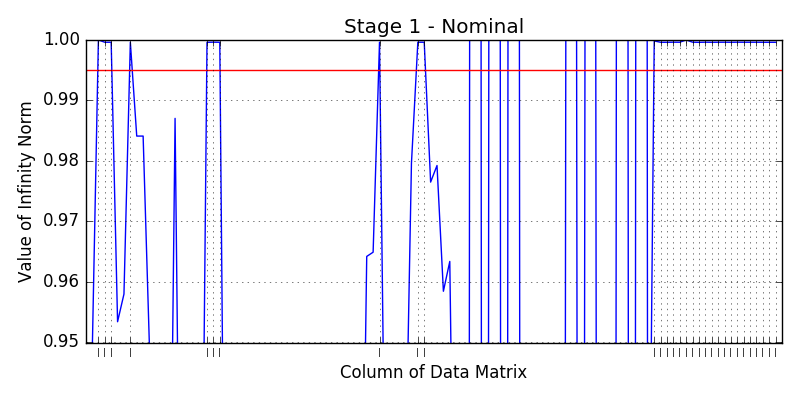
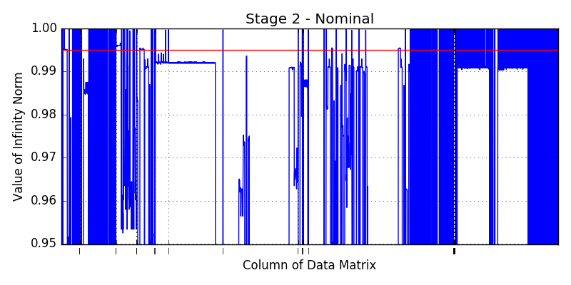
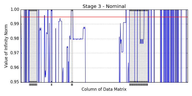
Figure 6: Here we show detection results for our three attack stages and detected using a RPCA based algorithm with a nominal $\lambda$ value as suggested in [10]. As in Figure 5, the red lines represent the detection threshold, the blue lines show the detected anomalies (which raise an alarm when the blue line is above the red detection threshold), and black dotted lines which mark the true attacks. As you can see, the RPCA algorithm with a nominal $\lambda$ value flags many normal packets as anomalous since the subspace it computed from the training data $Y_{0}$ is too low-dimensional.

Most importantly, in Figure 7, we show a RPCA analysis using a $\lambda=0.157$ which is approximately $15$ times larger than the nominal $\lambda=0.01096$ as in [10]. Of course, nothing in this text should be viewed as contradicting the results in [10]. However, we are solving a different problem. We are not focused on recovering a true low-rank $L$ and sparse $S$. In particular, it is not even clear what such a “true” low-rank $L$ and sparse $S$ would even mean in our case. Rather, we choose $\lambda$ to optimize our anomaly detection performance. In some sense, the $L$ we compute from our training data $Y_{0}$ is most appropriate for the computer network at hand and therefore our anomaly detection performance is improved.

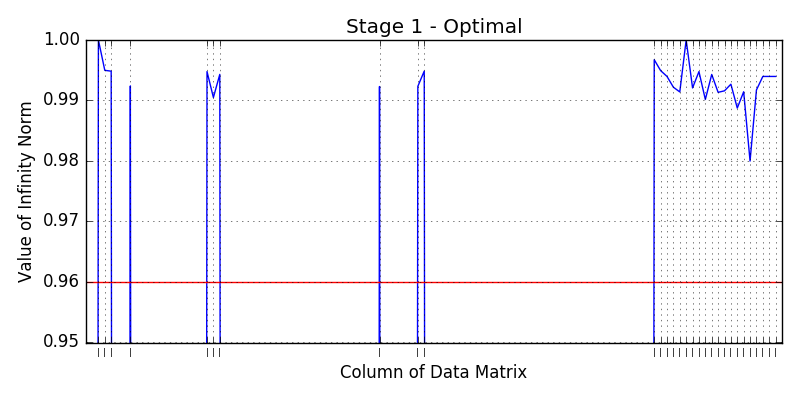
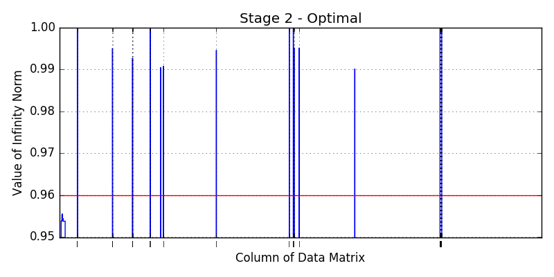
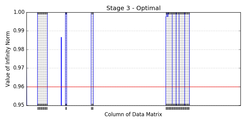
Figure 7: Here we show detection results for our three attack stages and detected using a RPCA based algorithm with an optimized value for $\lambda=0.157$. As in Figure 5 the red lines represent the detection threshold, the blue line shows the detected anomalies (which raise an alarm when the blue line is above the red detection threshold), and black dotted lines which mark the true attacks. This $\lambda$ value was optimized by training on stage one and two, so perhaps its efficacy in those stages is not overly surprising. However, $\lambda=0.157$ was not computed any information from stage three, yet using the same subspace computed from $Y_{0}$ (and $\lambda$ computed from stages one and two) gives rise to far fewer false positives and false negatives than the competing methods.

Finally, as observed in Section III-B we also need to train our anomaly detection threshold $\alpha$. Accordingly, in Figure 8 we show Receiver Operator Curves (ROC) for each of the stages as we vary the detection threshold $\alpha$ from $0$ to $1$. We show ROC curves for PCA, for RPCA using a nominal $\lambda=0.01096$, and for RPCA using an optimized $\lambda=0.157$. Again, the optimized $\lambda$ was chosen by training on the attacks in stage one and two, and therefore the good performance may not be surprising in that case. However, the results in stage three are not tuned for those specific attacks, and the optimized $\lambda$ still provides better performance in those cases across all threshold values $\alpha$.

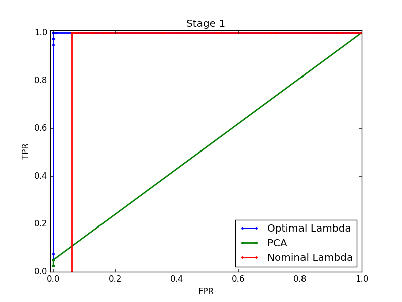
(a) Stage 1 ROC curve

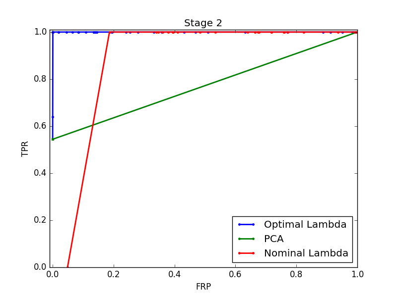
(b) Stage 2 ROC curve

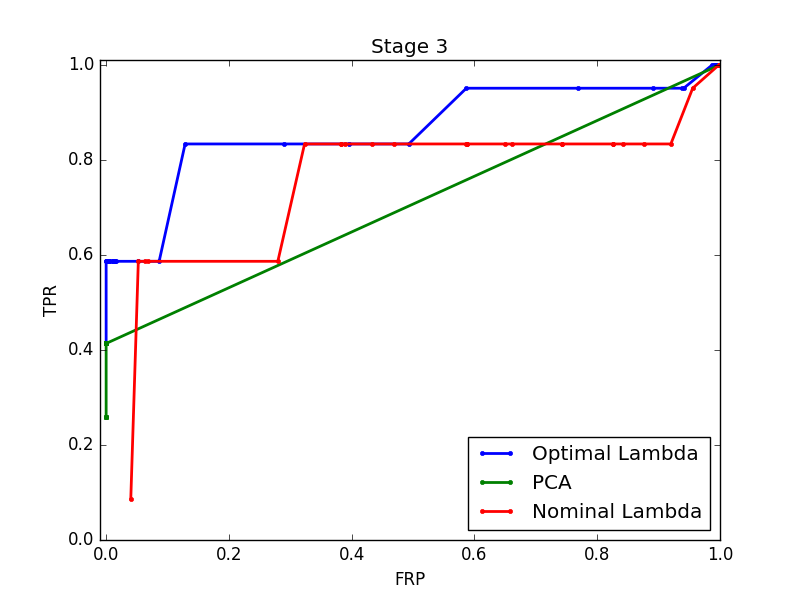
(c) Stage 3 ROC curve

Figure 8: Here we show ROC curves, parameterized by our detection threshold $\alpha$, for our three attack stages. For each attack stage we show the performance of PCA (shown in green), a nominal RPCA (shown in red), and an RPCA with a $\lambda$ value optimized on stage one and two (shown in blue). We train our optimal $\lambda$ value on the stage one and two attacks, so perhaps it is not surprising that the ROC for stage one and two in 8(a) shows superior performance for the optimized RPCA algorithm. However, the attack in stage 3 (in 8(c)) is quite different from the attack in stage 1. However, the ROC curves still demonstrate better performance for the trained $\lambda$ value, especially over a standard PCA approach.

V Conclusions

In this paper, we have demonstrated how a RPCA approach can be used to detect anomalies in PCAP data. In particular, we have shown that using training data to optimize just two parameters in the RPCA algorithm, can lead to substantially improved detection results in contrast to a PCA approach or a RPCA approach using the literature-recommended value for $\lambda$. We illustrated by example that one class of attacks could quite successfully detect a separate class of attacks. This result supports our original hypothesis that the low dimensional subspace computed by RPCA, even on training data, is more representative of the true nominal state of the measured data. This allows for a great range of anomalies, and hence network attacks, to be successfully detected.

References

- [1] Python Programming Language – Official Website. http://www.python.org/.
- [2] Atef Abdelkefi, Yuming Jiang, Wei Wang, Arne Aslebo, and Olav Kvittem. Robust traffic anomaly detection with principal component pursuit. Proceedings of the ACM CoNEXT Student Workshop on - CoNEXT ’10 Student Workshop, page 1, 2010.
- [3] Hervé Abdi and Lynne J. Williams. Principal component analysis, 2010.
- [4] Raven Alder, Josh Burke, Chad Keefer, Angela Orebaugh, Larry Pesce, and Eric S. Seagren. Introducing Wireshark. In How to Cheat at Configuring Open Source Security Tools, pages 297–335. 2007.
- [5] Usha Banerjee, Ashutosh Vashishtha, and Mukul Saxena. Evaluation of the Capabilities of WireShark as a tool for Intrusion Detection. International Journal of Computer Applications, 6(7):975–8887, 2010.
- [6] Stephen Boyd. Distributed Optimization and Statistical Learning via the Alternating Direction Method of Multipliers. Foundations and Trends® in Machine Learning, 3(1):1–122, 2010.
- [7] Daniela Brauckhoff, Kave Salamatian, and Martin May. Applying PCA for traffic anomaly detection: Problems and solutions. In Proceedings - IEEE INFOCOM, pages 2866–2870, 2009.
- [8] JF F Cai, EJ J Candès, and Z Shen. A singular value thresholding algorithm for matrix completion. SIAM Journal on Optimization, pages 1–28, 2010.
- [9] EJ Candès and B Recht. Exact matrix completion via convex optimization. Foundations of Computational Mathematics, 2009.
- [10] Emmanuel J Candès, Xiaodong Li, Yi Ma, John Wright, and Emmanuel J Candes. Robust Principal Component Analysis? Journal of the ACM, 58(3):1–37, 2009.
- [11] Emmanuel J Candes and Yaniv Plan. Matrix Completion With Noise. Proceedings of the IEEE, 98(6):11, 2009.
- [12] Venkat Chandrasekaran, Sujay Sanghavi, Pablo A. Parrilo, and Alan S. Willsky. Rank-Sparsity Incoherence for Matrix Decomposition. arXiv:0906.2220v1, jun 2009.
- [13] C Eckart and G Young. The approximation of one matrix by another of lower rank. Psychometrika, 1:211–218, 1936.
- [14] N Halko, PG Martinsson, and JA Tropp. Finding Structure with Randomness: Probabilistic Algorithms for Constructing Approximate Matrix Decompositions. SIAM review, 53(2):217–288, 2011.
- [15] Jerome Hastie, Trevor, Tibshirani, Robert, Friedman. The Elements of Statistical LearningData Mining, Inference, and Prediction, Second Edition. 2009.
- [16] Xuexiang Jin, Yi Zhang, Li Li, and Jianming Hu. Robust PCA-Based Abnormal Traffic Flow Pattern Isolation and Loop Detector Fault Detection. Tsinghua Science and Technology, 13(6):829–835, 2008.
- [17] Roland Kwitt and Ulrich Hofmann. Unsupervised Anomaly Detection in Network Traffic by Means of Robust PCA. 2007 International Multi-Conference on Computing in the Global Information Technology (ICCGI’07), pages 37–37, 2007.
- [18] Anukool Lakhina, Mark Crovella, and Christophe Diot. Diagnosing network-wide traffic anomalies. ACM SIGCOMM Computer Communication Review, 34(4):219, 2004.
- [19] Anukool Lakhina, Konstantina Papagiannaki, Mark Crovella, Christophe Diot, Eric D. Kolaczyk, and Nina Taft. Structural analysis of network traffic flows. ACM SIGMETRICS Performance Evaluation Review, 32(1):61, 2004.
- [20] Morteza Mardani, Gonzalo Mateos, and Georgios B. Giannakis. Dynamic anomalography: Tracking network anomalies via sparsity and low rank. IEEE Journal on Selected Topics in Signal Processing, 7(1):50–66, aug 2013.
- [21] Morteza (University of Minnesota) Mardani. Leveraging Sparsity and Low Rank for Large-Scale Networks and Data Science. PhD thesis, 2015.
- [22] RC Paffenroth, R Nong, and P Du Toit. On covariance structure in noisy, big data. SPIE Optical Engineering+ Applications, pages 88570E–88570E, 2013.
- [23] RC Paffenroth, PC Du Toit, LL Scharf, A. P. Jayasumana, V. Bandara, and Ryan Nong. Distributed pattern detection in cyber networks. In Cyber Sensing, volume 8393, 2012.
- [24] Claúdia Pascoal, M. Rosário De Oliveira, Rui Valadas, Peter Filzmoser, Paulo Salvador, and António Pacheco. Robust feature selection and robust PCA for internet traffic anomaly detection. Proceedings - IEEE INFOCOM, pages 1755–1763, 2012.
- [25] Haakon Ringberg, Augustin Soule, Jennifer Rexford, and Christophe Diot. Sensitivity of PCA for traffic anomaly detection. Proceedings of the 2007 ACM SIGMETRICS international conference on Measurement and modeling of computer systems SIGMETRICS 07, 35:109, 2007.
- [26] Chris Sanders. Practical Packet Analysis: using Wireshark to solve real-world network problems. Network Security, 2011(8):4, 2011.
- [27] Jonathon Shlens. A Tutorial on Principal Component Analysis. Tutorial, Salk Institute, pages 1–12, 2009.
- [28] John Wright, Arvind Ganesh, Shankar Rao, Yigang Peng, and Yi Ma. Robust Principal Component Analysis: Exact Recovery of Corrupted Low-Rank Matrices via Convex Optimization. In Advances in Neural Information Processing Systems, pages 2080–2088, 2009.
- [29] Huan Xu, Constantine Caramanis, and Sujay Sanghavi. Robust PCA via Outlier Pursuit. Computer, pages 1–29, 2010.