Adaptive Finite Element Solution of the Porous Medium Equation in Pressure Formulation

Abstract

A lack of regularity in the solution of the porous medium equation poses a serious challenge in its theoretical and numerical studies. A common strategy in theoretical studies is to utilize the pressure formulation of the equation where a new variable called the mathematical pressure is introduced. It is known that the new variable has much better regularity than the original one and Darcy’s law for the movement of the free boundary can be expressed naturally in this new variable. The pressure formulation has not been used in numerical studies. The goal of this work is to study its use in the adaptive finite element solution of the porous medium equation. The MMPDE moving mesh strategy is employed for adaptive mesh movement while linear finite elements are used for spatial discretization. The free boundary is traced explicitly by integrating Darcy’s law with the Euler scheme. Numerical results are presented for three two-dimensional examples. The method is shown to be second-order in space and first-order in time in the pressure variable. Moreover, the convergence order of the error in the location of the free boundary is almost second-order in the maximum norm. However, numerical results also show that the convergence order of the method in the original variable stays between first-order and second-order in the $L^{1}$ norm or between 0.5th-order and first-order in the $L^{2}$ norm. Nevertheless, the current method can offer some advantages over numerical methods based on the original formulation for situations with large exponents or when a more accurate location of the free boundary is desired.

• Key words:  porous medium equation, adaptive moving mesh method, MMPDE method, finite element method, free boundary, Darcy’s law, pressure formulation

• AMS subject classifications:  65M60, 65M50, 35Q35

1 Introduction

We consider the numerical solution of the two-dimensional (2D) porous medium equation (PME)

$$u_{t}=\nabla\cdot(|u|^{m}\nabla u),$$ (1)

where $m$ is a physical parameter whose value and physical meaning depend on a specific application. PME is a nonlinear and nontrivial extension of the classic heat equation and arises in many applications including the modeling of gas flow through porous media, boundary layer theory for fluid dynamics, image processing, and particle physics. An important feature of PME is its degeneracy: the diffusion coefficient vanishes wherever the solution becomes zero. This induces the finite propagation property in the sense that the solution of PME is compactly supported at all time if it is so initially. The boundary of the compact support becomes a free boundary, propagating at a finite speed governed by Darcy’s law. Moreover, the boundary is becoming smoother while the solution itself is losing its regularity at the free boundary as time evolves. Mathematical studies for PME began in 1950s; for example, see Oleĭnik et al. [27], Kalašnikov [24], and Aronson [2]. Significant progress has been made since the late 1980s; e.g. see Herrero et al. [17], Shmarev [30], and the monograph of Vázquez [32].

PME has been a challenge for numerical simulation due to its lack of regularity and free boundary. The finite element method (FEM) has been used on fixed uniform or quasi-uniform meshes and error estimates have been established in, e.g., Rose [28], Nochetto and Verdi [26], Rulla and Walkington [29], Ebmeyer [14], and Wei and Lefton [33]. Although applicable to two and higher dimensions, most of these results are not optimal. In particular, they state that the convergence order for P1 finite elements is at most first-order and decreases as the parameter $m$ increases. On the other hand, due to the dynamic nature of free boundary and the low solution regularity thereon, it is natural to employ dynamically adaptive meshes for the numerical solution of PME. For this reason, there has been a trend in using adaptive moving mesh methods for PME since 1990s. For example, Budd et al. [7] study the numerical simulation of self-similarity solutions of one-dimensional PME using the Moving Mesh PDE (MMPDE) method [21, 22] with a monitor function designed to preserve scaling invariance. Baines et al. [3, 4, 5] develop a moving mesh linear FEM for PME that locally conserves the mass in the initial solution. For the situation with $m=1$, their method achieves an optimal convergence order for both the 1D and 2D cases. However, it does not produce an optimal convergence order for $m>1$. An exception can be made in 1D with a special initial mesh, which leads to second-order convergence for the case $m=3$. Unfortunately, this initial mesh has not yet been attempted in 2D due to its high computational cost. More recently, Duque et al. [11, 12, 13] apply an MMPDE method to PME having variable exponent (where $m$ depends on location and time) and with or without absorption terms and show first-order convergence of the method for 2D problems. Ngo and Huang [25] study the MMPDE method with linear finite elements for a general form of PME (with constant or variable exponents and with or without absorption terms) in a large domain that contains the solution support for the whole time period under consideration. The method is shown to be able to handle problems with complex, emerging, or splitting free boundaries and be second-order in convergence in space when the mesh adaptation is based on the Hessian of the approximate solution. While FEM has been a common choice for PME, other methods have also been studied, including the finite difference method by Socolovsky [31], the local discontinuous Galerkin method by Zhang and Wu [34], and the spectral Galerkin method by Barrera [6]. Especially, the local discontinuous Galerkin method of [34] is very successful, which gives high order of convergence within the solution support (away from the free boundary) and completely eliminates unwanted oscillations at the free boundary, although it has yet to be applied in 2D.

The form of (1), which will hereafter be referred to as the original formulation or simply PME-U, has been used in all of the existing numerical works so far. A drawback of this formulation is that its solution $u$ has a steep or infinite slope at the free boundary. On the other hand, it is a common practice to use the mathematical pressure $v:={u^{m}}/{m}$ in theoretical studies of PME (e.g., see [1, 8, 9, 10]) since $v$ has much better regularity than $u$. For the Barenblatt-Pattle solution of PME, for example, $v$ is Lipschitz continuous in $\boldsymbol{x}$ and $t$ and $\nabla v$ is bounded in the support of the solution (see [32]). Using the new variable $v$, we can rewrite (1) into

$$v_{t}=\nabla\cdot(mv\nabla v)-(m-1)|\nabla v|^{2},$$ (2)

which will be referred to as PME-V hereafter. Compared to (1), (2) is no longer in the divergence form for $m\neq 1$. However, its solution has higher regularity than that of PME-U, as mentioned earlier. Moreover, as will be seen later, the equation governing the movement of the free boundary can be expressed naturally in $v$.

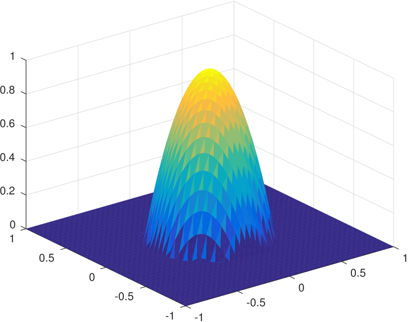
(a) Embedding approach.

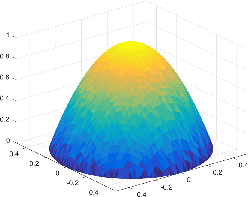
(b) Nonembedding approach.

Figure 1: Two approaches for solving free boundary problems.

When dealing with free or moving boundary problems, there are two main numerical approaches in general. The first, which can be called the “embedding” or “immersed boundary” approach, performs computations on a fixed but generally large domain which contains the support of the solution at all time of the simulation (cf. Fig. 1(a)). Although more memory and more CPU time are required for covering the extra domain outside the solution support and the solution usually has lower regularity across the free boundary, this approach does not need to explicitly trace the free boundary and is very robust for handling situations with complex free boundaries or topological changes (such as merging or splitting) in free boundaries. This approach has been used in, for example, [11, 25, 31, 34] for the numerical solution of PME. The other approach, which can be called the “nonembedding” approach, solves PME only within the solution support (see an illustration in Fig. 1(b)). The main challenge of this approach is to trace the free boundary (denoted by $\Gamma(t)$) via Darcy’s law (e.g. see Shmarev [30])

$$\Gamma^{\prime}(t)=-\lim_{\boldsymbol{x}\to\Gamma(t)^{-}}\nabla\left(\frac{u^{m}}{m}\right)\cdot{\boldsymbol{n}},$$ (3)

where $\Gamma^{\prime}(t)$ is the velocity of the free boundary and ${\boldsymbol{n}}$ is its unit outward normal. Note that the boundary is part of the solution to be sought. Moreover, once the boundary moves, the mesh points should be redistributed or adjusted accordingly. This approach has been used in [3, 4, 5, 7, 12, 13] with moving mesh methods.

The objective of this paper is to study the numerical solution of PME in the PME-V formulation using the nonembedding approach. The PME-V formulation has not been used in the past in the numerical simulation of PME. As mentioned earlier, its solution has better regularity. Moreover, noticing that the term in the parentheses in (3) is actually $v$, we can express the equation naturally in $v$ as

$$\Gamma^{\prime}(t)=-\lim_{\boldsymbol{x}\to\Gamma(t)^{-}}\nabla v\cdot{\boldsymbol{n}}.$$ (4)

With this, the initial-boundary value problem of PME in the PME-V formulation reads as

$$\begin{cases}v_{t}=\nabla\cdot(mv\nabla v)-(m-1)|\nabla v|^{2}\,,\quad&\text{in}\quad\Omega(t),\quad t\in(t_{0},T]\\ v(\boldsymbol{x},t_{0})=v_{0}(\boldsymbol{x})\,,\quad&\text{in}\quad\Omega(t_{0})\\ v(\boldsymbol{x},t)=0\,,\quad&\text{on}\quad\partial\Omega(t)\,,\quad t\in(t_{0},T]\\ \Gamma^{\prime}(t)=\displaystyle-\lim_{\boldsymbol{x}\to\Gamma(t)^{-}}\nabla v(\boldsymbol{x},t)\cdot{\boldsymbol{n}},&\text{on}\quad\partial\Omega(t)\,,\quad t\in(t_{0},T]\end{cases}$$ (5)

where $\Omega(t)$ denotes the support of the solution at time $t$ and $\partial\Omega(t)=\Gamma(t)$. We will explore the advantages and disadvantages of the PME-V formulation in the numerical solution of PME and study how well the MMPDE moving mesh method [21, 22] fares with this formulation. Recall that the latter has been used in [25] for the PME-U formulation with the embedding approach. It has been shown that the MMPDE method is able to concentrate the mesh points around the free boundary for the PME-U formulation and can lead to second-order convergence for some cases with linear finite elements. We will investigate if this is still true for the PME-V formulation.

The outline of the paper is as follows. Section 2 describes the moving mesh finite element method, involving the mesh generation via the MMPDE approach and the linear finite element discretization of PME. Numerical results obtained for three 2D examples are given in Section 3. Conclusions are drawn in Section 4. The reader is referred to [25] for a summary of mathematical properties of PME that are relevant to the numerical study or [32] for a more complete list of mathematical properties of PME.

2 The moving mesh finite element method

In this section we describe the moving mesh FE solution of PME-V (5) based on the MMPDE method. The discretization is based on the nonembedding approach which requires to trace the free boundary explicitly at each time level using Darcy’s law.

2.1 The MMPDE method

We describe a dynamical mesh generation method based on the MMPDE method [21]. The computation is performed on the moving domain $\Omega(t)$ which is partitioned at each time $t$ by a moving mesh $\mathcal{T}_{h}(t)$, always having $N_{v}$ vertices (denoted by $\boldsymbol{x}_{i}(t):i=1,\ldots,N_{v}$), $N$ elements, and a fixed connectivity. In addition, assuming that the first $N_{vi}$ vertices are interior vertices, we can then denote $\Gamma_{h}(t)=\{\boldsymbol{x}_{i}:i=N_{vi}+1,\ldots,N_{v}\}$ as a discretization of the boundary $\Gamma(t)$. We further assume that the numerical solution is obtained at the time instants

$$t_{0}<t_{1}<\ldots<t_{n_{f}}\equiv T,$$ (6)

and denote related quantities at time level $t=t_{n}$ by $\Omega^{n}$, $\mathcal{T}_{h}^{n}$, $\Gamma_{h}^{n}$, and $\{\boldsymbol{x}_{i}^{n}:i=1,\ldots,N_{v}\}$. Let the approximate solution at $t=t_{n}$ be $v_{h}^{n}$. Our goal is to generate a new mesh $\mathcal{T}_{h}^{n+1}$ for the computation of the solution $v_{h}^{n+1}$ at the new time level $t=t_{n+1}$. To this end, we first move the free boundary according to Darcy’s law (4). For simplicity, we use the Euler scheme to move boundary vertices in the normal direction, i.e.,

$$\boldsymbol{x}_{i}^{n+1}=\boldsymbol{x}_{i}^{n}-\left.\left((\nabla_{h}v_{h}^{n})\cdot{\boldsymbol{n}}\right){\boldsymbol{n}}\right|_{\boldsymbol{x}_{i}^{n}}(t_{n+1}-t_{n}),\quad i=N_{vi}+1,\ldots,N_{v}$$ (7)

where $\nabla_{h}v_{h}^{n}$ is an average of the gradient of $v_{h}$ in the neighboring elements of $\boldsymbol{x}_{i}^{n}$. After the boundary nodes are updated, we obtain a new intermediate physical mesh $\mathcal{\tilde{T}}_{h}^{n+1}$.

We apply the MMPDE method to generate the new physical mesh $\mathcal{T}_{h}^{n+1}$ based on $\mathcal{\tilde{T}}_{h}^{n+1}$ and $v_{h}^{n}$. The goal of the method is to make $\mathcal{T}_{h}^{n+1}$ to be as uniform as possible when viewed in the Riemannian metric specified by a matrix-valued function $\mathbb{M}$. We call such a mesh an $\mathbb{M}$-uniform mesh. The metric tensor $\mathbb{M}$ can be chosen based on error estimates, physical or geometric considerations, or combined. For our situation, we want more mesh points to concentrate around the free boundary. Recall that the solution $v$ is smooth around the free boundary and using the gradient or curvature of $v$ to define the metric tensor will not serve the purpose. For this reason, we define

$$\mathbb{M}=\frac{1}{\sqrt{(v_{h}^{n})^{2}+10^{-5}}}\;\mathbb{I},$$ (8)

with which more mesh points will be placed in regions where $v_{h}^{n}$ is small (i.e., regions around the free boundary). The threshold $10^{-5}$ is chosen by trial and error. Its choice is not very sensitive but cannot be too large (which will concentrate less mesh points near the free boundary) or too small (which will concentrate too many mesh points near the free boundary).

Having defined the metric tensor, we now discuss the MMPDE formulation. For the moment, we denote the computational mesh by $\mathcal{T}_{c}$ and the targeting physical mesh by $\mathcal{T}_{h}$, which are assumed to have the same numbers of elements and vertices and the same connectivity as $\mathcal{T}_{h}^{n}$. It has been shown (e.g., see [22]) that an $\mathbb{M}$-uniform mesh satisfies the equidistribution and alignment conditions

$$|K|\sqrt{\det(\mathbb{M}_{K})}=\frac{\sigma_{h}|K_{c}|}{|\Omega_{c}|},\quad\forall K\in\mathcal{T}_{h}$$ (9)

$$\frac{1}{d}\text{trace}\left(\left(F^{\prime}_{K}\right)^{-1}\mathbb{M}_{K}^{-1}\left(F^{\prime}_{K}\right)^{-T}\right)=\det\left(\left(F^{\prime}_{K}\right)^{-1}\mathbb{M}_{K}^{-1}\left(F^{\prime}_{K}\right)^{-T}\right)^{\frac{1}{d}},\quad\forall K\in\mathcal{T}_{h}$$ (10)

where $d$ is the dimension of $\Omega$ ($d=2$ for the current situation), $|K|$ and $|K_{c}|$ are the volumes of $K$ and its counterpart $K_{c}\in\mathcal{T}_{c}$, respectively, $\det(\cdot)$ and $\text{trace}(\cdot)$ denote the determinant and trace of a matrix, respectively, $\mathbb{M}_{K}$ is the average of $\mathbb{M}$ over $K$, $F^{\prime}_{K}$ is the Jacobian matrix of the affine mapping $F_{K}:K_{c}\to K$, and

$$\sigma_{h}=\sum_{K\in\mathcal{T}_{h}}|K|\sqrt{\det(\mathbb{M}_{K})},\quad|\Omega_{c}|=\sum_{K_{c}\in\mathcal{T}_{c}}|K_{c}|.$$

The equidistribution condition (9) requires that all of the elements have the same volume in the metric specified by $\mathbb{M}$. It determines the size of the elements through $\mathbb{M}$. On the other hand, the alignment condition (10) requires that $K$, when viewed in the metric $\mathbb{M}$, be similar to $K_{c}$ which is viewed in the Euclidean metric. It determines the shape and orientation of $K$ through $\mathbb{M}$ and the shape and orientation of $K_{c}$.

A mesh that closely satisfies the equidistribution and alignment condition can be obtained by minimizing

$$I_{h} =\theta\sum_{K\in\mathcal{T}_{h}}|K|\sqrt{\det(\mathbb{M}_{K})}\left(\text{trace}({(F_{K}^{\prime})}^{-1}{\mathbb{M}}_{K}^{-1}{(F_{K}^{\prime})}^{-T})\right)^{\frac{dp}{2}}$$

$$\quad\quad+(1-2\theta)d^{\frac{dp}{2}}\sum_{K\in\mathcal{T}_{h}}|K|\sqrt{\det(\mathbb{M}_{K})}\left(\frac{|K_{c}|}{|K|\sqrt{\det(\mathbb{M}_{K})}}\right)^{p},$$ (11)

where $\theta\in(0,\frac{1}{2}]$ and $p>1$ are non-dimensional parameters. The function (11) is a discrete form of the continuous functional developed in [18] that combines the equidistribution and alignment conditions. Numerical experiment shows that the choice $\theta=1/3$ and $p=2$ works for most problems, which we will use in our computation. Due to its high nonlinearity, solving the minimization problem for (11) is a nontrivial task. We use here the MMPDE method (a time-transient approach) to solve the problem. Notice that $I_{h}$ is a function of the coordinates of the computational vertices ($\boldsymbol{\xi}_{j},\;j=1,...,N_{v}$) and the physical vertices ($\boldsymbol{x}_{j},\;j=1,...,N_{v}$). Moreover, recall that our goal is to generate a new physical mesh $\mathcal{T}_{h}^{n+1}$. It is straightforward to solve for $\boldsymbol{x}_{j},\;j=1,...,N_{v}$ directly for a given reference computational mesh $\mathcal{T}_{c}$. The formulas for this so-called $\boldsymbol{x}$-formulation of the MMPDE method are given in [19, Equation (39)-(41)] but omitted here to save space. It is proven in [20] that the mesh governed by this formulation stays nonsingular all the time if it is nonsingular initially. This result holds at semi- and fully-discrete levels and for convex and concave domains in any dimension. However, the metric tensor $\mathbb{M}$ is defined on the physical domain and a function of $\boldsymbol{x}_{j},\;j=1,...,N_{v}$, which increases the nonlinearity of $I_{h}$. Even worse, $\mathbb{M}$ is typically known only on the previous mesh $\mathcal{T}_{h}^{n}$. As a result, $\mathbb{M}$ needs to be updated constantly during the minimization process when the physical mesh varies all the time. To avoid these difficulties, we use here an indirect approach (the $\boldsymbol{\xi}$-formulation of the MMPDE method) with which we take $\mathcal{T}_{h}=\mathcal{\tilde{T}}_{h}^{n+1}$ (which is basically the physical mesh at the previous step and fixed during the minimization process), minimize $I_{h}$ to obtain a new computation mesh, and finally obtain $\mathcal{T}_{h}^{n+1}$ through interpolation. Notice that $I_{h}$ now is a function of $\boldsymbol{\xi}_{j},\;j=1,...,N_{v}$ only. Then the MMPDE for the computational vertices is defined as the gradient system of $I_{h}$ as

$$\frac{d\boldsymbol{\xi}_{j}}{dt}=-\frac{P_{j}}{\tau}\left[\frac{\partial I_{h}}{\partial\boldsymbol{\xi}_{j}}\right]^{T},\quad j=1,...,N_{v}$$ (12)

where the row vector ${\partial I_{h}}/{\partial\boldsymbol{\xi}_{j}}$ is the derivative of $I_{h}$ with respect to $\boldsymbol{\xi}_{j}$, $\tau>0$ is a parameter used to adjust how fast the mesh movement reacts to any change in the metric tensor, and $P_{j}=\det(\mathbb{M}(\boldsymbol{x}_{j}))^{\frac{p-1}{2}}$ is chosen such that (12) is invariant under the scaling transformation of $\mathbb{M}$: $\mathbb{M}\to c\,\mathbb{M}$ for any positive constant $c$. The derivative ${\partial I_{h}}/{\partial\boldsymbol{\xi}_{j}}$ can be found analytically using the notion of scalar-by-matrix differentiation [19]. Using this, we can rewrite (12) into

$$\frac{d\boldsymbol{\xi}_{j}}{dt}=\frac{P_{j}}{\tau}\sum_{K\in\omega_{j}}|K|\boldsymbol{v}_{j_{K}}^{K},\quad j=1,\dotsc,N_{v}$$ (13)

where $\omega_{j}$ denotes the element patch associated with the vertex $\boldsymbol{x}_{j}$, $j_{K}$ is the local index of the same vertex on the element $K$, and $\boldsymbol{v}_{j_{K}}^{K}$ is the velocity contributed by $K$ to the vertex $\boldsymbol{x}_{j}$. Each element $K$ contributes a velocity $\boldsymbol{v}_{i}^{K}$ to its vertex $\boldsymbol{x}_{i}^{K}$ ($i=0,\ldots,d$). These local velocities are given by

$$\begin{bmatrix}{(\boldsymbol{v}_{1}^{K})}^{T}\\ \vdots\\ {(\boldsymbol{v}_{d}^{K})}^{T}\end{bmatrix}=-E_{K}^{-1}\frac{\partial G}{\partial\mathbb{J}}-\frac{\partial G}{\partial\det(\mathbb{J})}\frac{\det(\hat{E}_{K})}{\det(E_{K})}\hat{E}_{K}^{-1},\quad\boldsymbol{v}_{0}^{K}=-\sum_{i=1}^{d}\boldsymbol{v}_{d}^{K},$$ (14)

where $E_{K}=[\boldsymbol{x}_{1}^{K}-\boldsymbol{x}_{0}^{K},...,\boldsymbol{x}_{d}^{K}-\boldsymbol{x}_{0}^{K}]$ and $\hat{E}_{K}=[{\boldsymbol{\xi}}_{1}^{K}-{\boldsymbol{\xi}}_{0}^{K},...,{\boldsymbol{\xi}}_{d}^{K}-\boldsymbol{\xi}_{0}^{K}]$ are the edge matrices of $K$ and $K_{c}$, respectively, $\mathbb{J}=(F_{K}^{\prime})^{-1}$, the function $G$ that is associated with (11) has the form

$$G(\mathbb{J},\det(\mathbb{J}),\mathbb{M})=\theta\sqrt{\det(\mathbb{M})}\left(\text{trace}(\mathbb{J}\mathbb{M}^{-1}\mathbb{J}^{T})\right)^{\frac{dp}{2}}+(1-2\theta)d^{\frac{dp}{2}}\sqrt{\det(\mathbb{M})}\left(\frac{\det(\mathbb{J})}{\sqrt{\det(\mathbb{M})}}\right)^{p},$$

and the derivatives $\frac{\partial G}{\partial\mathbb{J}}$ and $\frac{\partial G}{\partial\det(\mathbb{J})}$ are given by

$$\frac{\partial G}{\partial\mathbb{J}}=dp\theta\sqrt{\det(\mathbb{M})}\left(\text{trace}(\mathbb{J}\mathbb{M}^{-1}\mathbb{J}^{T})\right)^{\frac{dp}{2}-1}\mathbb{M}^{-1}\mathbb{J}^{T},$$

$$\frac{\partial G}{\partial\det(\mathbb{J})}=p(1-2\theta)d^{\frac{dp}{2}}\det(\mathbb{M})^{\frac{1-p}{2}}\det(\mathbb{J})^{p-1}.$$

Note that these derivatives are evaluated at $(\mathbb{J},\det(\mathbb{J}),\mathbb{M})=((F_{K}^{\prime})^{-1},\det(F_{K}^{\prime})^{-1},\mathbb{M}_{K})$.

The above mesh velocities should be modified for boundary vertices. For instance, they should be set to be zero for fixed boundary vertices. If boundary vertices are allowed to slid on the boundary, additional constraints should be applied so that they do not move inside or outside the domain.

The system (13), with proper modifications for the boundary vertices, can be integrated from $t=t_{n}$ to $t=t_{n+1}$ to get the new computational mesh $\mathcal{T}_{c}^{n+1}$, with the initial mesh at $t=t_{n}$ taken to be the reference computational mesh $\mathcal{T}_{c,h}$ which can be chosen as a quasi-uniform mesh for $\Omega(t_{0})$. We use Matlab’s ODE solver ode15s for this purpose. Since $\mathcal{T}_{c}^{n+1}$ has the same structure (i.e., the same number of elements and vertices and the same connectivity) as the physical mesh $\mathcal{\tilde{T}}_{h}^{n+1}$, there is a piecewise affine map $\Phi_{h}^{n+1}$ such that $\mathcal{\tilde{T}}_{h}^{n+1}=\Phi_{h}^{n+1}(\mathcal{T}_{c}^{n+1})$. From this, we can compute the new physical mesh as $\mathcal{T}_{h}^{n+1}=\Phi_{h}^{n+1}(\mathcal{T}_{c,h})$ using linear interpolation.

2.2 Linear finite element discretization on moving meshes

In this subsection we describe the moving mesh FE method and the procedure for solving (5) on moving meshes. We first notice that we now have the old mesh $\mathcal{T}_{h}^{n}$, the new mesh $\mathcal{T}_{h}^{n+1}$, and the physical solution $v_{h}^{n}$ defined on $\mathcal{T}_{h}^{n}$. For any $t\in[t_{n},t_{n+1}]$, we define the mesh $\mathcal{T}_{h}(t)$ as the one having the same structure as $\mathcal{T}_{h}^{n}$ and $\mathcal{T}_{h}^{n+1}$ and with the coordinates of the vertices as

$$\boldsymbol{x}_{j}(t)=\frac{t-t_{n}}{t_{n+1}-t_{n}}\boldsymbol{x}_{j}^{n+1}+\frac{t_{n+1}-t}{t_{n+1}-t_{n}}\boldsymbol{x}_{j}^{n},\quad j=1,...,N_{v}.$$

The corresponding nodal mesh velocities are given by

$$\dot{\boldsymbol{x}}_{j}(t)=\frac{\boldsymbol{x}_{j}^{n+1}-\boldsymbol{x}_{j}^{n}}{t_{n+1}-t_{n}},\quad j=1,...,N_{v}.$$

The linear basis function $\phi_{j}(\boldsymbol{x},t)$ associated with vertex $\boldsymbol{x}_{j}$ satisfies

$$\phi_{j}|_{K}\in\mathbb{P}_{1}\quad\forall K\in\mathcal{T}_{h}(t),\quad\text{and}\quad\phi_{j}(\boldsymbol{x}_{i},t)=\delta_{ij},\quad i=1,\ldots,N_{v}.$$

We can then define the moving finite element space as

$$V_{h}(t)=\text{span}\{\phi_{1}(\cdot,t),...,\phi_{N_{vi}}(\cdot,t)\}\,,\quad t\in(t_{n},t_{n+1})$$

and the linear finite approximation to (5) as $v_{h}(\cdot,t)\in V_{h}(t),\,t\in(t_{n},t_{n+1}]$ such that

$$\int_{\Omega(t)}\frac{\partial v_{h}}{\partial t}\psi~{}d\boldsymbol{x}=-m\int_{\Omega(t)}v_{h}\nabla v_{h}\cdot\nabla\psi~{}d\boldsymbol{x}+(1-m)\int_{\Omega(t)}|\nabla v_{h}|^{2}\psi~{}d\boldsymbol{x},\quad\forall\psi\in V_{h}(t).$$ (15)

We need to pay special attention to the time derivative $\frac{\partial v_{h}}{\partial t}$ in the above equation. Expressing $v_{h}$ into

$$v_{h}(\cdot,t)=\sum_{j=1}^{N_{vi}}v_{j}(t)\phi_{j}(\cdot,t)$$ (16)

and differentiating it with respect to $t$, we have

$$\frac{\partial v_{h}}{\partial t}=\sum_{j=1}^{N_{v_{i}}}\frac{dv_{j}}{dt}\phi_{j}(\boldsymbol{x},t)+\sum_{j=1}^{N_{v_{i}}}v_{j}(t)\frac{\partial\phi_{j}}{\partial t}.$$

It can be shown (e.g., see Jimack and Wathen [23, Lemma 2.3]) that

$$\frac{\partial\phi_{j}}{\partial t}=-\nabla\phi_{j}\cdot\dot{\boldsymbol{X}},$$

where $\dot{\boldsymbol{X}}$ is a piecewise linear mesh velocity function defined as $\dot{\boldsymbol{X}}(\boldsymbol{x},t)=\sum_{j=1}^{N_{v}}\dot{\boldsymbol{x}}_{j}(t)\phi_{j}(\boldsymbol{x},t)$. Combining these we get

$$\frac{\partial v_{h}}{\partial t}=\sum_{j=1}^{N_{v_{i}}}\frac{dv_{j}}{dt}\phi_{j}(\boldsymbol{x},t)-\nabla v_{h}\cdot\dot{\boldsymbol{X}}.$$ (17)

Substituting (16) and (17) into (15) and taking $\psi=\phi_{i},\,i=1,\ldots,N_{vi}$ successively, we get

$$\sum_{j=1}^{N_{vi}}\left(\int_{\Omega(t)}\phi_{j}\phi_{i}~{}d\boldsymbol{x}\right)\frac{dv_{j}}{dt}= \int_{\Omega(t)}\nabla v_{h}\cdot\left(\dot{\boldsymbol{X}}\phi_{i}-mv_{h}\nabla\phi_{i}\right)~{}d\boldsymbol{x}$$

$$+(1-m)\int_{\Omega(t)}|\nabla v_{h}|^{2}\phi_{i}~{}d\boldsymbol{x},\quad i=1,...,N_{vi}$$

which can be written into the matrix form as

$$B(\boldsymbol{X})\dot{\boldsymbol{V}}=F(\boldsymbol{V},\boldsymbol{X},\dot{\boldsymbol{X}}),$$ (18)

where $B$ is the mass matrix and $\boldsymbol{X}$ and $\boldsymbol{V}$ are vectors representing the mesh and solution, respectively. The ODE system (18) is integrated from $t_{n}$ to $t_{n+1}$ using the fifth-order Radau IIA method (an implicit Runge-Kutta method) with a standard time step selection procedure where the relative and absolute tolerance are chosen as $10^{-6}$ and $10^{-8}$, respectively, and the error estimation is based on a two-step error estimator of Gonzalez-Pinto et al. [16].

To conclude this section, we summarize the entire procedure for solving (5) in the following.

1. Partition and approximate $\Omega(t_{0})$ with the initial mesh $\mathcal{T}_{h}^{0}$. We choose $\mathcal{T}_{c,h}=\mathcal{T}_{h}^{0}$ as our reference computational mesh for the MMPDE moving mesh method. Assume that at time level $t=t_{n}$, we have the solution $v_{h}^{n}$ on the mesh $\mathcal{T}_{h}^{n}$.

2. Use the scheme (7) for Darcy’s law to the boundary $\Gamma^{n}$ to obtain the new boundary $\Gamma^{n+1}$. This new boundary reflects the new domain $\Omega_{h}^{n+1}$ and is incorporated into the physical mesh $\mathcal{\tilde{T}}_{h}^{n+1}$.

3. Apply the MMPDE method with the mesh $\mathcal{\tilde{T}}_{h}^{n+1}$ and its corresponding solution $v_{h}^{n}$ to get the new physical mesh $\mathcal{T}_{h}^{n+1}$ at time level $t=t_{n+1}$.

4. Apply the moving mesh FE method with $v_{h}^{n}$, $\mathcal{T}_{h}^{n}$, and $\mathcal{T}_{h}^{n+1}$ to obtain the new solution $v_{h}^{n+1}$ at time level $t=t_{n+1}$.

5. Repeat steps (ii) to (iv) until the final time $t=T$ is reached.

One can see that the boundary movement, the mesh movement, and the update of the physical solution are split and performed sequentially. We thus expect that the method is first-order in time. On the other hand, the physical PDE is discretized with linear finite elements and we expect the method to be second-order in space when the solution is sufficiently smooth.

3 Numerical results

In this section we present numerical results obtained with the moving mesh method described in the previous section for IBVP (5). Unless otherwise stated, we choose the parameter $\tau$ of the MMPDE equation (12) to depend on the number of mesh elements $N$, i.e.,

$$\tau=\min\left\{10^{-3},\frac{10^{-1}}{N}\right\}.$$ (19)

Moreover, we restrict the time step to be no greater than $10^{-4}$, namely,

$$\Delta t_{max}:=\max_{n=1,\,\ldots\,,\,n_{f}}(t_{n}-t_{n-1})\leq 10^{-4}.$$ (20)

These choices are made by trial and error. They produce satisfactory results for the problems we have tested.

      Example 3.1 (Barenblatt-Pattle solution).

In this example we consider the well-known Barenblatt-Pattle (BP) solution for PME-V given by

$$v(r,t)=\begin{cases}\frac{1}{m\lambda^{dm}(t)}\left(1-\left(\frac{r}{r_{0}\lambda(t)}\right)^{2}\right),\quad&\text{for}\quad|r|\leq r_{0}\lambda(t)\\ 0,\quad&\text{for}\quad|r|>r_{0}\lambda(t)\end{cases}$$ (21)

where

$$r=|\boldsymbol{x}|,\quad\lambda(t)=\left(\frac{t}{t_{0}}\right)^{\frac{1}{2+dm}},\quad t_{0}=\frac{r_{0}^{2}m}{2(2+dm)}\,,$$ (22)

and $r_{0}>0$ is a parameter representing the radius of the solution support at the initial time $t_{0}$. This solution is radially symmetric, self-similar, and compactly supported for any finite time. It has been used as a benchmark example to test numerical algorithms for PME. Notice that the BP solution (in terms of $v$) is smooth on its support (including the regions near the boundary) for any parameter $m$, as can be seen in Fig. 2.

(a) $m=2$

(b) $m=3$

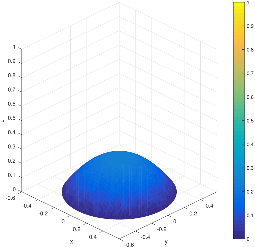
(c) $m=4$

Figure 2: The Barenblatt-Pattle special solution for PME-V (5) is plotted for $m=2$, $3$, and $4$.

The moving mesh method is applied with $T=(t_{0}+0.1)/2$ and $r_{0}=0.5$ (with $t_{0}$ defined in (22)). A typical mesh and its associated solution are plotted in Fig. 3. One can see that the mesh points are concentrated correctly around the free boundary. This is a demonstration of the mesh adaptation capability of the numerical method. A convergence history (as the number of mesh elements $N$ increases) for both the solution and the boundary is given in Fig. 4 for $m=2,\,3,\,4$, and $5$. The $L^{2}$-norm of the error converges with a second-order rate (in terms of the average element diameter $h=1/\sqrt{N}$) for all considered values of $m$. (A similar convergence behavior is also observed in the $L^{1}$-norm.) The convergence order of the error in the boundary location, measured in the $L^{\infty}$-norm, is almost second-order. One may notice that these errors are smaller for higher $m$. A closer examination shows that there are no oscillations in the computed solutions. To see how accurate the computed solution in the original variable is, we obtain $u$ using the computed $v$ and compare it with the exact solution. The convergence history in $u$ is shown in Fig. 5 for both the $L^{1}$ and $L^{2}$-norms. It can be seen that the convergence order in this variable in $L^{2}$-norm is about first-order for $m=2$ and deteriorates as $m$ increases, which is indeed consistent with theoretical estimates in literature (e.g. [14, 26, 28, 29, 33]). Interestingly, the error in the $L^{1}$-norm has a better convergence rate, almost second-order for $m=2$ and 1.5th-order for $m=5$.

We now study the effects of large $m$ on the computation. Recall that the solution $u$ of PME-U formulation has a steeper or infinite slope at the free boundary as $m$ increases. Due to this, numerical methods based on PME-U generally have difficulties to deal with large $m$ situations. For example, the MMPDE moving mesh FE method in [25] can lead to second-order convergence in the $L^{2}$ norm of error in $u$ for small $m$ ($m<5$) but has difficulty to maintain the same convergence order for large $m$ ($m\geq 5$). This is because, in the latter situation, the mesh elements have to be extremely stretched near the free boundary which can cause the time integration of PME to stop due to too small time steps. On the other hand, $m$ has nearly no effects on the computation of PME-V and the convergence order in $v$ stays almost the same (second-order) for all $m$; see Fig. 4(a) for $m=2,\,3,\,4$, and $5$ and Fig. 6(a) for much higher $m=8,\;9,\;10$, and $15$. The convergence order of the error in the boundary location stays almost second-order too for large $m$ (cf. Fig. 6(b)). However, the convergence order in the $u$ computed through $v$ becomes close to 0.5th-order in $L^{2}$ norm and first-order in $L^{1}$ norm for very large $m$; see Fig. 7(a,b).

It is interesting to see how the time step size affects the accuracy of the computed solution. We use a relatively fine mesh with $N=40459$ and a sequence of $\Delta t_{max}$. The error is shown in Fig. 8. One can see that the error remains constant for small $\Delta t_{max}$ because the total error is dominated by the spatial discretization error when the time step is small. On the other hand, for larger $\Delta t_{max}$, the error decreases at a rate between first-order and second-order. The overall convergence is more like first-order, which is consistent with our expectation from the construction of the numerical method. ∎

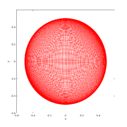
(a) Mesh

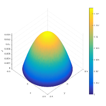
(b) Computed solution

Figure 3: Example 3.1. The final mesh and computed solution are plotted for $m=3$ ($N=40459$).

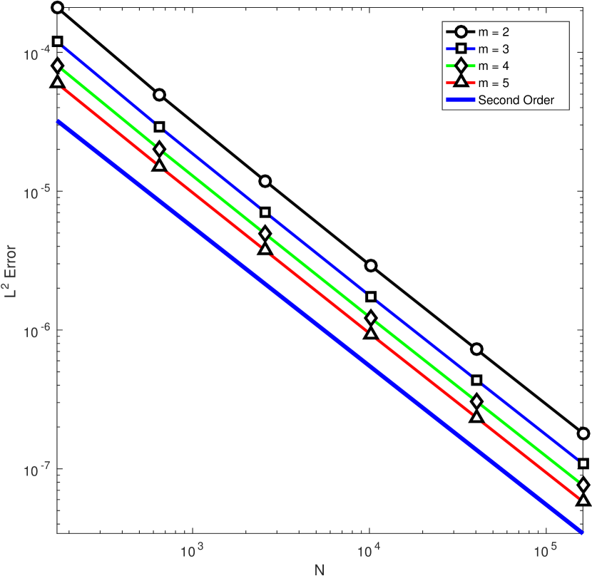
(a) $L^{2}$ error of solution

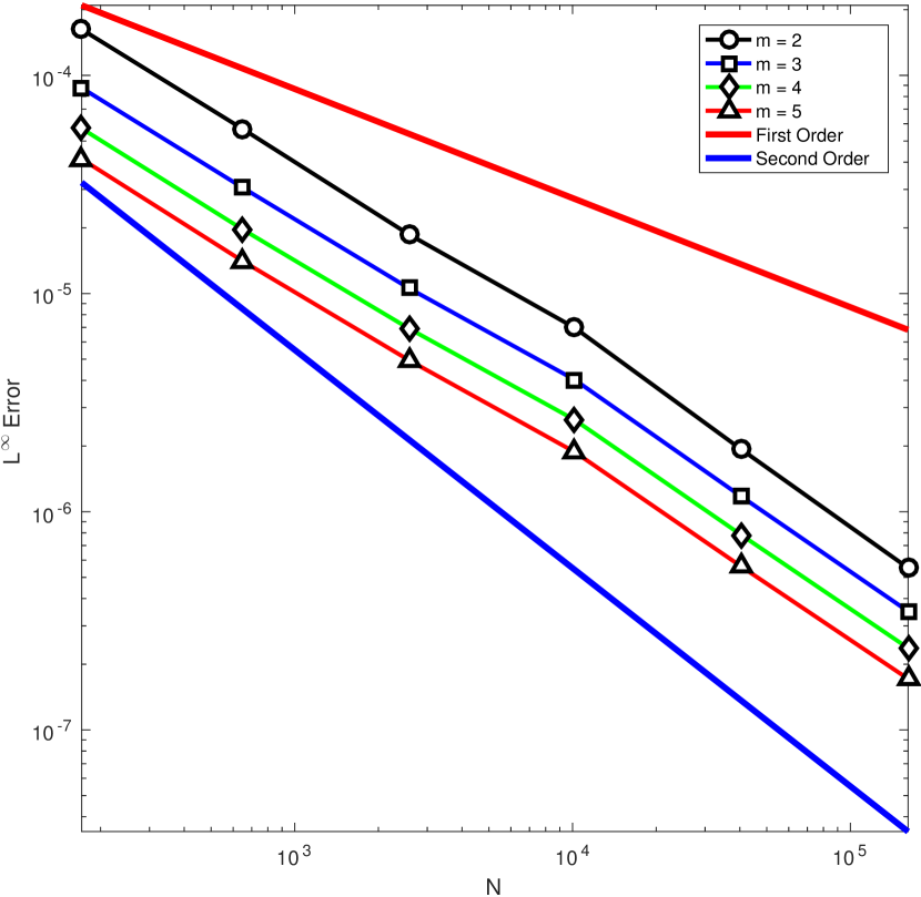
(b) $L^{\infty}$ error of the boundary

Figure 4: Example 3.1. Convergence histories of the moving mesh method ($v$-variable).

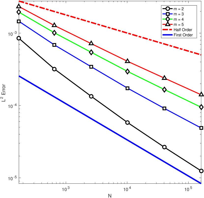
(a) $L^{2}$ Error

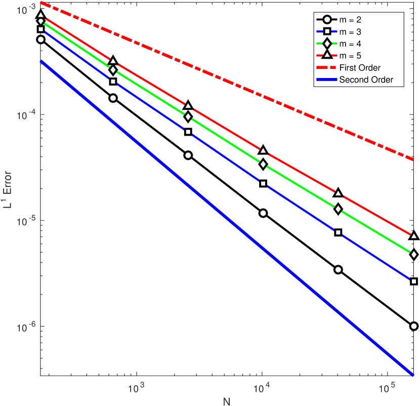
(b) $L^{1}$ Error

Figure 5: Example 3.1. Convergence history of the method in the original $u$-variable.

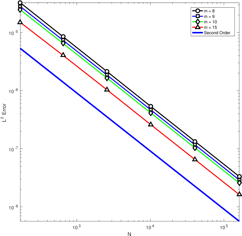
(a) $L^{2}$ error of solution

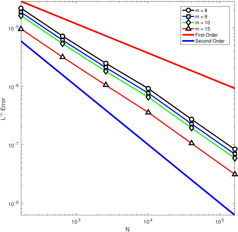
(b) $L^{\infty}$ error of the boundary

Figure 6: Example 3.1. Convergence histories of the moving mesh method ($v$-variable) for $m=8,\;9,\;10$, and $15$.

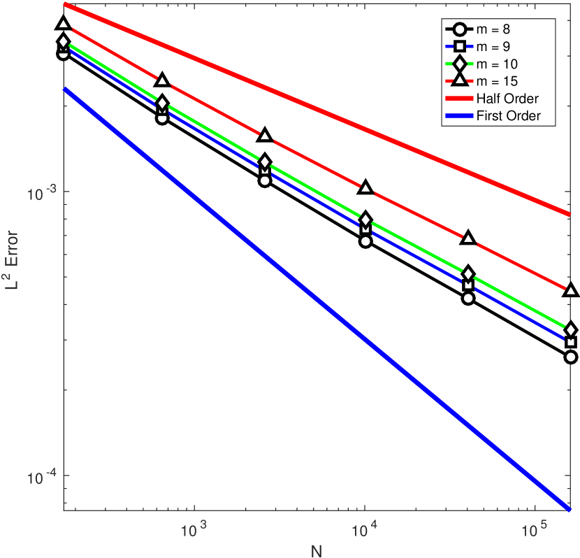
(a) $L^{2}$ Error

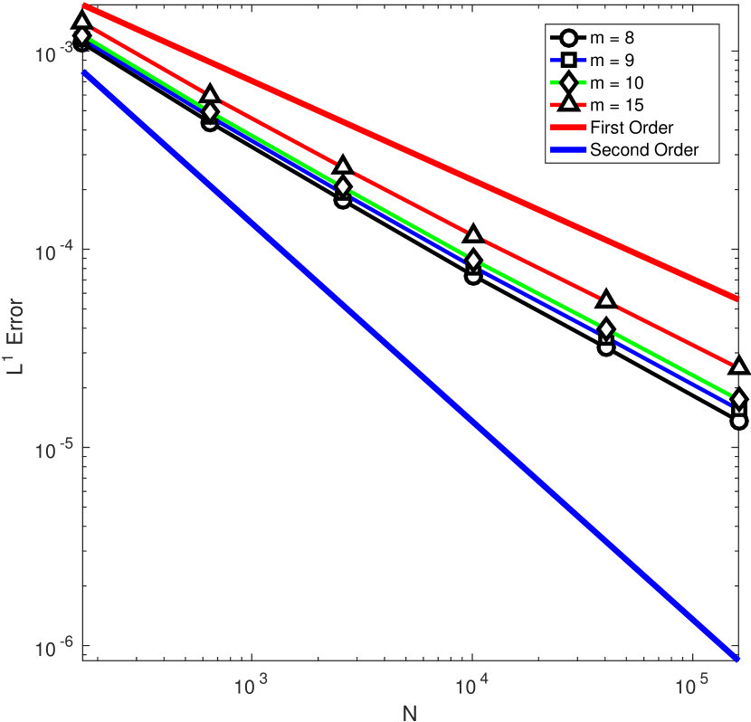
(b) $L^{1}$ Error

Figure 7: Example 3.1. Convergence history of the method in the original $u$-variable for $m=8,\;9,\;10$, and $15$.

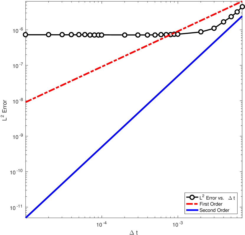
(a) $L^{2}$ Error of solution

(b) A closer look

Figure 8: Example 3.1 with $m=2$. Error history of the moving mesh method ($v$-variable) when compared with fixed time steps.

      Example 3.2 (Waiting time phenomenon).

It is known that for some initial solutions, the IBVP (5) exhibits the waiting-time phenomenon where the free boundary does not move initially until a finite amount of time has elapsed. Consider an example with $m=2$ and the initial solution

$$v_{0}(x,y)=\begin{cases}\frac{1}{m}\cos^{m}\left(\sqrt{x^{2}+y^{2}}\right),&\quad\text{for}\quad\sqrt{x^{2}+y^{2}}\leq\frac{\pi}{2}\\ 0,&\quad\text{otherwise}.\end{cases}$$ (23)

We observe that

$$\nabla\left(\frac{1}{m}\cos^{m}\left(\sqrt{x^{2}+y^{2}}\right)\right)=-\frac{\cos^{m-1}(\sqrt{x^{2}+y^{2}})\,\sin(\sqrt{x^{2}+y^{2}})}{\sqrt{x^{2}+y^{2}}}\begin{bmatrix}x\\ y\end{bmatrix},$$

which vanishes at $\sqrt{x^{2}+y^{2}}=\frac{\pi}{2}$. According to Darcy’s law (4), the velocity of the free boundary is zero, and thus we should not expect the free boundary to move initially. In Fig. 9, the mesh and associated solution are plotted at several instants (with contrasting circles representing the initial boundary). To further confirm the waiting-time phenomenon, we also plot the cross sections of the solution at various time instants in Fig. 10. A closer look suggests that the free boundary does not start moving until around $t=0.2$. Moreover, no oscillations are visible in the computed solutions. This is in contrast with embedding methods which typically produce computed solutions with small oscillations near the free boundary; e.g., see [25, Fig. 12]. ∎

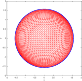
(a) $t=0.11$

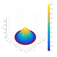
(b) $t=0.11$

(c) $t=0.2$

(d) $t=0.2$

(e) $t=0.3$

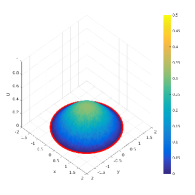
(f) $t=0.3$

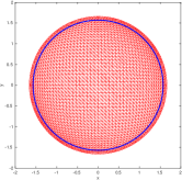
(g) $t=0.8$

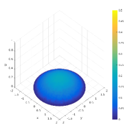
(h) $t=0.8$

Figure 9: Example 3.2. The mesh and computed solution are shown at various time instants ($N=4011$). The contrasting circles represent the initial boundary.

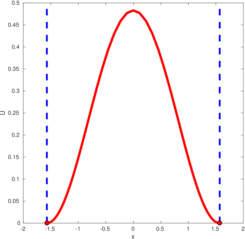
(a) $t=0.11$

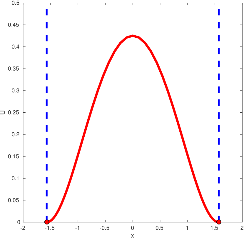
(b) $t=0.15$

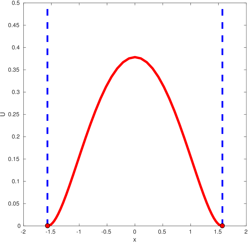
(c) $t=0.20$

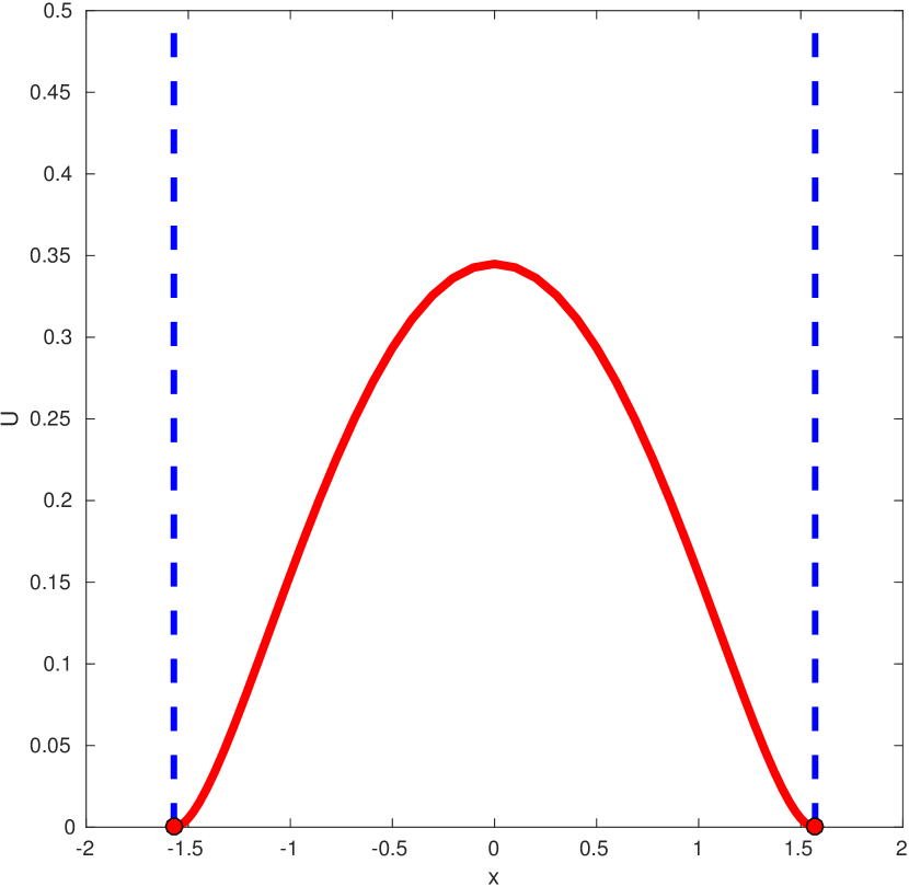
(d) $t=0.25$

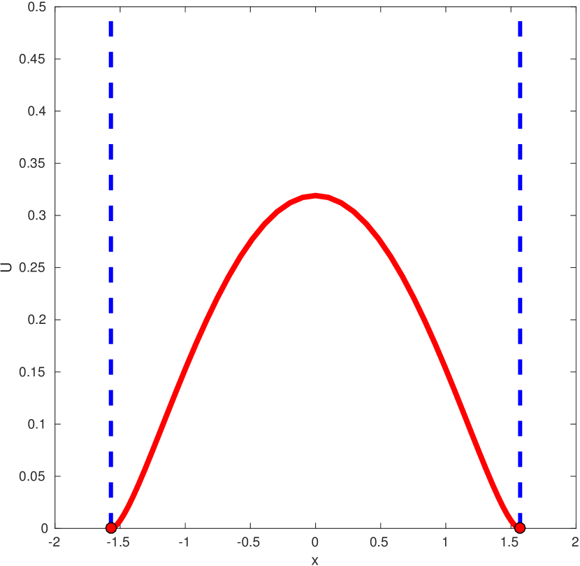
(e) $t=0.30$

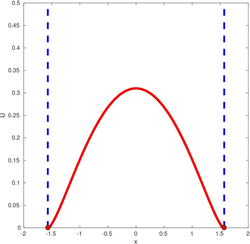
(f) $t=0.32$

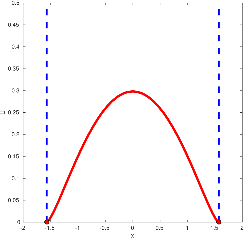
(g) $t=0.35$

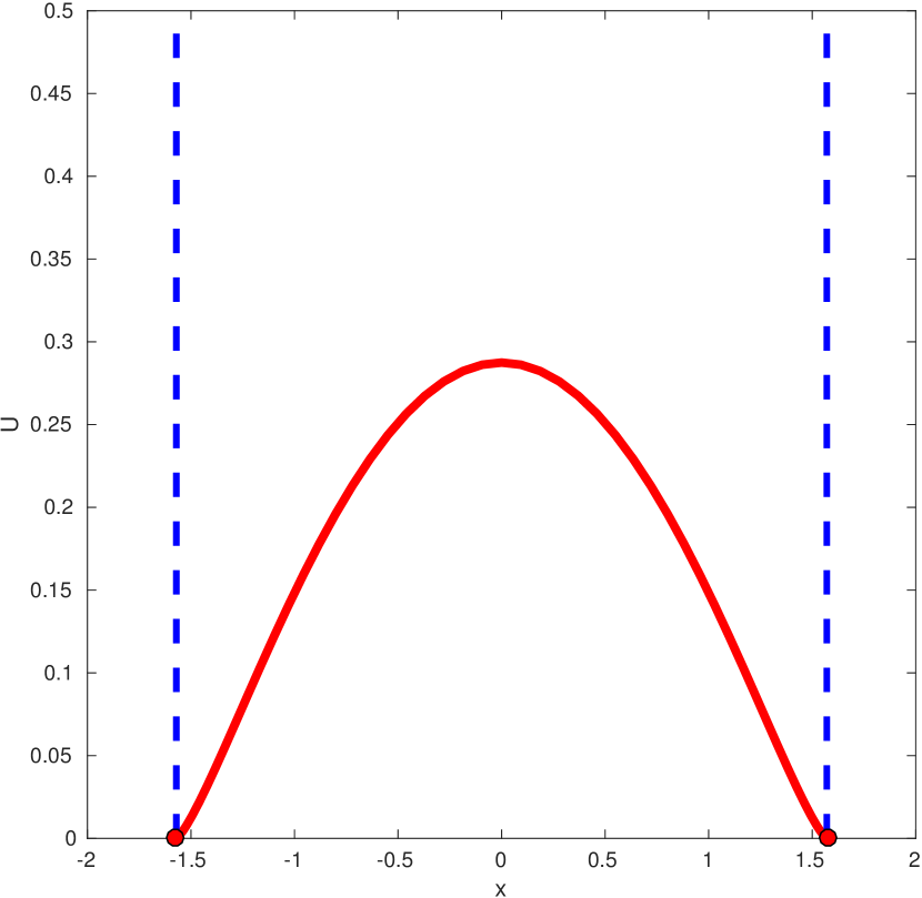
(h) $t=0.38$

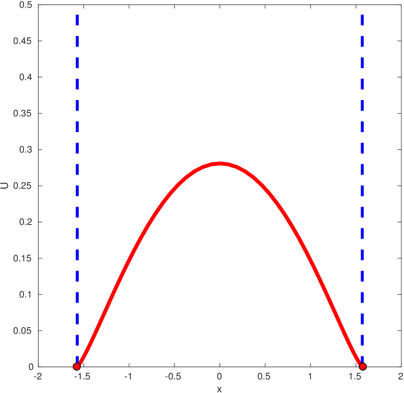
(i) $t=0.40$

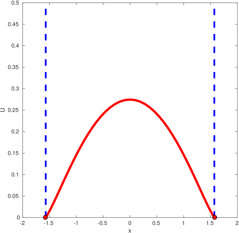
(j) $t=0.42$

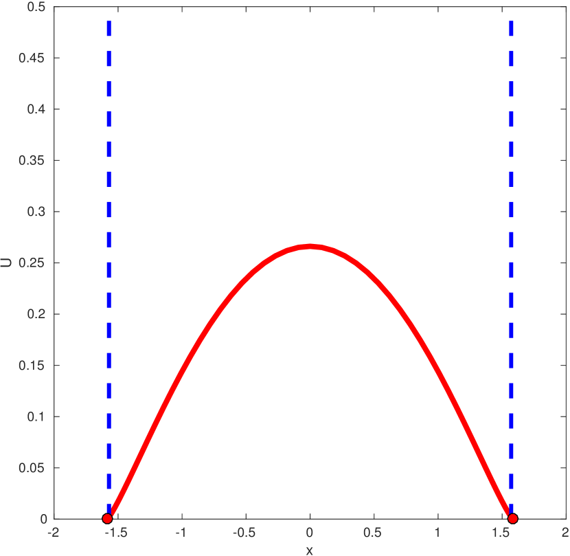
(k) $t=0.45$

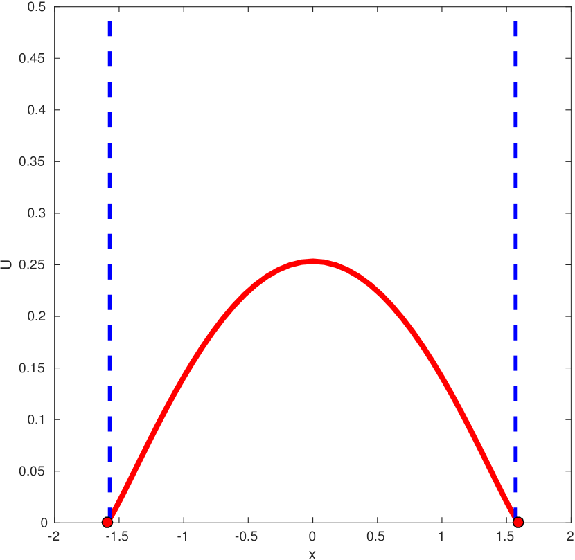
(l) $t=0.50$

(m) $t=0.60$

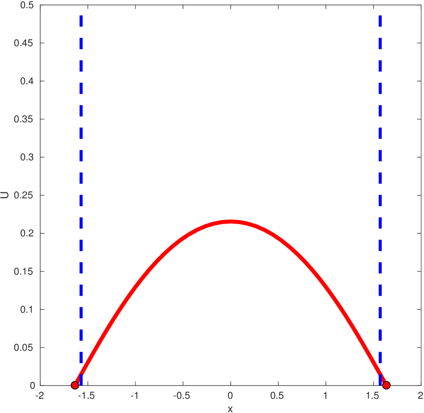
(n) $t=0.70$

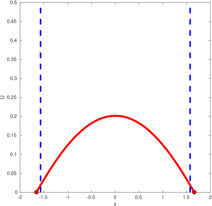
(o) $t=0.80$

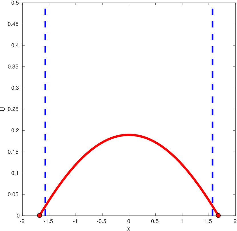
(p) $t=0.90$

Figure 10: Example 3.2. The cross section at $y=0$ of a computed solution is shown at various time instants ($N=4011$).

      Example 3.3 (Complex domain).

In this example we apply our method to PME-V with $m=2$ and

$$v_{0}(x,y)=\begin{cases}25\left[0.25^{2}-(\sqrt{x^{2}+y^{2}}-0.75)^{2}\right]^{\frac{3}{2}},&\quad\text{for}\quad\sqrt{x^{2}+y^{2}}\in[0.5,1]\text{ and }(x<0\text{ or }y<0)\\ 25\left[0.25^{2}-x^{2}-(y-0.75)^{2}\right]^{\frac{3}{2}},&\quad\text{for}\quad x^{2}+(y-0.75)^{2}\leq 0.25^{2}\text{ and }x\geq 0\\ 25\left[0.25^{2}-(x-0.75)^{2}-y^{2}\right]^{\frac{3}{2}},&\quad\text{for}\quad(x-0.75)^{2}+y^{2}\leq 0.25^{2}\text{ and }y\geq 0\\ 0,&\quad\text{otherwise}.\end{cases}$$ (24)

The partial donut-shaped support pertaining to this initial solution is first seen in Baines et al. [4]. Fig. 11 shows a representative mesh and the corresponding solution. One can see that the mesh evolves smoothly following the evolving free boundary. The simulation does not encounter any difficulty until the hole closes out and the boundary begins to touch. This example also demonstrates that the MMPDE moving mesh method works well for concave domains (without causing any mesh tangling or crossing). ∎

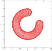
(a) $t=0.1$

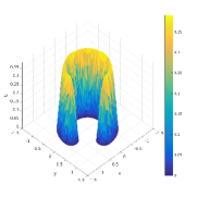
(b) $t=0.1$

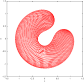
(c) $t=0.3$

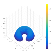
(d) $t=0.3$

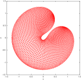
(e) $t=0.75$

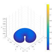
(f) $t=0.75$

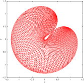
(g) $t=1$

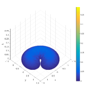
(h) $t=1$

Figure 11: Example 3.3. A computed solution is shown at various time instants ($N=4011$).

4 Conclusions

In the previous sections we have studied the adaptive finite element solution of PME in the pressure formulation (PME-V) (2). The motivation is that the pressure variable $v=u^{m}/m$ has better regularity than $u$ and the equation for the movement of the free boundary can be expressed naturally in $v$. In fact, many theoretical works (e.g., [1, 8, 9, 10]) have relied on PME-V to obtain mathematical properties for $u$. But PME-V has not been used in numerical studies of PME in the past. We have used PME-V in a nonembedding approach with which PME is discretized only within the support of the solution and the free boundary is traced explicitly via Darcy’s law (4). This approach, though not as robust as the embedding methods (e.g. [11, 25, 31, 34]) in dealing with problems having complex free boundaries, offers better solution regularity, leads to more accurate location of the free boundary, and avoids unwanted oscillations in computed solutions. We have employed the boundary-mesh-physical splitting solution procedure where the boundary equation (Darcy’s law) is first solved using the Euler scheme, then the mesh is updated, and finally PME is solved using piecewise line finite elements on the moving mesh. The MMPDE moving mesh method has been used for mesh updating. Since $v$ is smooth near the free boundary in the current situation, a $v$-value based metric tensor (8) has been used to control the mesh concentration near the boundary.

Numerical results obtained with the moving mesh finite element method have been presented for three two-dimensional examples. They show that the method can effectively concentrate mesh points near the free boundary without causing any mesh tangling or crossing for both convex and concave domains. Moreover, no oscillations have been observed in the computed solutions. Furthermore, the error in $v$ shows a convergence rate of second order in space and first order in time. Finally, the error in the location of the free boundary exhibits almost second-order convergence in the $L^{\infty}$ norm. Interestingly, these convergence behaviors are essentially independent of $m$ for its tested range from $2$ to $15$. It is noted that the original variable $u$ can be obtained from the computed solution through the definition $u=(mv)^{1/m}$. However, the convergence in the so-computed $u$ is not satisfactory. As a matter of fact, the convergence order is between 0.5th-order and first-order and closer to 0.5th-order for large $m$ in the $L^{2}$ norm and is between first-order and second-order and close to first-order for large $m$ in the $L^{1}$ norm.

Recall that the embedding moving mesh finite element method developed in [25] based on the original formulation (PME-U) is able to handle problems with complex, emerging, or splitting free boundaries and is second-order in space in $u$ for relatively small $m$. For large $m$, it can run into difficulties since the mesh elements have to be stretched extremely thin near the free boundary which can cause the time integration of PME to stop due to too small time steps. Comparing these with the observations made in this work, we can conclude that PME-V can offer advantages over PME-U for situations with large $m$ or when a more accurate location of the free boundary is desired. For other situations, numerical methods based on the original formulation can be more advantageous.

References

- [1] S. Angenent. Analyticity of the Interface of the porous media equation after the waiting time. Proc. Amer. Math. Soc., 102: 329–336, 1988.
- [2] D. G. Aronson. Regularity properties of flows through porous media. SIAM J. Appl. Math., 17:461–467, 1969.
- [3] M. J. Baines, M. E. Hubbard, and P. K. Jimack. A moving mesh finite element algorithm for fluid flow problems with moving boundaries. I. J. Numer. Meth. Fluids, 47:1077–1083, 2005. 8th ICFD Conference on Numerical Methods for Fluid Dynamics. Part 2.
- [4] M. J. Baines, M. E. Hubbard, and P. K. Jimack. A moving mesh finite element algorithm for the adaptive solution of time-dependent partial differential equations with moving boundaries. Appl. Numer. Math., 54:450–469, 2005.
- [5] M. J. Baines, M. E. Hubbard, P. K. Jimack, and A. C. Jones. Scale-invariant moving finite elements for nonlinear partial differential equations in two dimensions. Appl. Numer. Math., 56:230–252, 2006.
- [6] J. H. Barrera A spectral Galerkin approximation of the porous medium equation. Cornell University. PhD Thesis, 2011.
- [7] C. Budd, G. Collins, W. Huang, and R. D. Russell. Self-similar numerical solutions of the porous medium equation using moving mesh methods. Phil. Trans. R. Soc. Lond. A, 357:1047–1078, 1999.
- [8] L. A. Caffarelli and A. Friedman. Regularity of the free boundary of a gas flow in an -dimensional porous medium. Indiana Univ. Math. J., 29:361–391, 1980.
- [9] L. A. Caffarelli, J. L. Vazquez, and N. I. Wolanski. Lipschitz Continuity of solutions and interfaces of the N-dimensional porous medium equation. Indiana Univ. Math. J., 36:373–401, 1987.
- [10] P. Daskalopoulos and R. Hamilton. Regularity of the free boundary for the porous medium equation. J. Amer. Math. Soc., 11:899–965, 1998.
- [11] J. C. M. Duque, R. M. P. Almeida, and S. N. Antontsev. Convergence of the finite element method for the porous media equation with variable exponent. SIAM J. Numer. Anal., 51(6):3483–3504, 2013.
- [12] J. C. M. Duque, R. M. P. Almeida, and S. N. Antontsev. Numerical study of the porous medium equation with absorption, variable exponents of nonlinearity and free boundary. Appl. Math. Comput., 235:137–147, 2014.
- [13] J. C. M. Duque, R. M. P. Almeida, and S. N. Antontsev. Application of the moving mesh method to the porous medium equation with variable exponent. Math. Comput. Simulation, 118:177–185, 2015.
- [14] C. Ebmeyer. Error estimates for a class of degenerate parabolic equations. SIAM J. Numer. Anal., 35:1095–1112, 1998.
- [15] C. Ebmeyer and W. B. Liu. Finite element approximation of the fast diffusion and the porous medium equations. SIAM J. Numer. Anal., 46:2393–2410, 2008.
- [16] S. González-Pinto, J. I. Montijano, and S. Pérez-Rodríguez. Two-step error estimators for implicit Runge-Kutta methods applied to stiff systems. ACM Trans. Math. Software, 30:1–18, 2004.
- [17] M. A. Herrero and J. L. Vázquez. The one-dimensional nonlinear heat equation with absorption: Regularity of solutions and interfaces. SIAM J. Math. Anal., 18:149–167, 1987.
- [18] W. Huang. Variational mesh adaptation: isotropy and equidistribution. J. Comput. Phys., 174:903–924, 2001.
- [19] W. Huang and L. Kamenski. A geometric discretization and a simple implementation for variational mesh generation and adaptation. J. Comput. Phys., 301:322–337, 2015.
- [20] W. Huang and L. Kamenski. On the mesh nonsingularity of the moving mesh PDE method. Math. Comp. (in press) (DOI: 10.1090/mcom/3271).
- [21] W. Huang, Y. Ren, and R. D. Russell. Moving mesh partial differential equations (MMPDEs) based upon the equidistribution principle. SIAM J. Numer. Anal., 31:709–730, 1994.
- [22] W. Huang and R. D. Russell. Adaptive Moving Mesh Methods. Springer, New York, 2011. Applied Mathematical Sciences Series, Vol. 174.
- [23] P. K. Jimack and A. J. Wathen. Temporal derivatives in the finite-element method on continuously deforming grids. SIAM J. Numer. Anal., 28:990–1003, 1991.
- [24] A. S. Kalašnikov. Formation of singularities in solutions of the equation of nonstationary filtration. Z̆. Vyčisl. Mat. i Mat. Fiz., 7:440–444, 1967.
- [25] C. Ngo and W. Huang. A Study on Moving Mesh Finite Element Solution of the Porous Medium Equation. J. Comput. Phys., 331:357–380, 2017.
- [26] R. H. Nochetto and C. Verdi. Approximation of degenerate parabolic problems using numerical integration. SIAM J. Numer. Anal., 25:784–814, 1988.
- [27] O. A. Oleĭnik, A. S. Kalašinkov, and Y. Čžou. The Cauchy problem and boundary problems for equations of the type of non-stationary filtration. Izv. Akad. Nauk SSSR. Ser. Mat., 22:667–704, 1958.
- [28] M. E. Rose. Numerical methods for flows through porous media. I. Math. Comp., 40:435–467, 1983.
- [29] J. Rulla and N. J. Walkington. Optimal rates of convergence for degenerate parabolic problems in two dimensions. SIAM J. Numer. Anal., 33:56–67, 1996.
- [30] S. Shmarev. Interfaces in solutions of diffusion-absorption equations in arbitrary space dimension. In Trends in partial differential equations of mathematical physics, volume 61 of Progr. Nonlinear Differential Equations Appl., pages 257–273. Birkhäuser, Basel, 2005.
- [31] E. A. Socolovsky On numerical methods for degenerate parabolic problems. Carnegie Mellon University. PhD Thesis, 1984.
- [32] J. L. Vázquez. The porous medium equation. Oxford Mathematical Monographs. The Clarendon Press, Oxford University Press, Oxford, 2007. Mathematical theory.
- [33] D. Wei and L. Lefton. A priori error estimates for Galerkin approximations to porous medium and fast diffusion equations. Math. Comp., 68:971–989, 1999.
- [34] Q. Zhang and Z.-L. Wu. Numerical simulation for porous medium equation by local discontinuous Galerkin finite element method. J. Sci. Comput., 38:127–148, 2009.