Time Dependent Geometry in Massive Gravity

Abstract

In this paper, we will analyze a time dependent geometry in a massive theory of gravity. This will be done by analyzing Vaidya spacetime in such a massive theory of gravity. As gravitational collapse is a time dependent system, we will analyze it using the Vaidya spacetime in massive gravity. The Vainshtein and dRGT mechanisms are used to obtain a ghost free massive gravity, and construct such time dependent solutions. Singularities formed, their nature and strength will be studied in detail. We will also study the thermodynamical aspects of such a geometry by calculating the important thermodynamical quantities for such a system, and analyzing the thermodynamical behavior of such quantities.

1 Introduction

The observations from type I supernovae indicate that our universe is in a state of accelerated cosmic expansion [1]-[6]. This accelerated cosmic expansion can be explained by a cosmological constant term in the Einstein equation, and the existence of such a cosmological constant is predicted from all quantum field theories. However, the cosmological constant paradigm suffers from two well known problems as the “cosmological constant problem” and the “coincidence problem”. These problems have motivated the people to do research in the dark energy models [7]-[9] and the modified theories of gravity [10]. The latter theories are constrained by the solar system tests [11]-[12], where the modifications have to occur only at the infrared limit. It is possible to obtain an infrared modification of the general relativity by making the gravitons massive [13], such that the small graviton mass does not violate the known experimental bounds. Even though this has been done by adding a small Fierz-Pauli mass term to the original action of general relativity [14]-[15], there are problems with the zero mass limit of this theory due to the force mediated by the scalar graviton. Furthermore, such a modified theory of gravity violates the experimental bounds obtained from solar system experiments, and so it cannot be a physical theory [11]-[12].

It was possible to resolve these problems by using the Vainshtein mechanism, which was based on the inclusion of non-linear terms in the field equation [16]-[17]. Even though the Vainshtein mechanism produces the general relativity in suitable limits, it contains higher derivative terms. These higher derivative terms give rise to negative norm Boulware-Deser ghosts [18]. This problem can also be resolved for a subclass of massive potentials, as it has been observed that for such a subclass of massive potential the Boulware-Deser ghosts do not appear [19]-[25]. This has been done using dRGT mechanism, which is a theory with one dynamical and one fixed metric [26]. It is interesting to note that a mass term in the gravitational action can also be generated from the spontaneous breaking of Lorentz symmetry at the cosmological scale. [27]-[30]. Thus, the massive gravity might be produced by some interesting theoretical considerations.

As massive gravity produces interesting deformation of the general relativity, it has been used to study the behavior of various interesting systems. The black holes in Gauss-Bonnet massive gravity have been studied [31]-[32], and it has been demonstrated that the inclusion of mass term produces interesting deformation of these black holes. The thermodynamics of such black holes has been studied in the extended phase space [13]-[33]. It has been demonstrated that the phase transition of black holes depends on the different parameters used in this massive gravity [33]. Cosmological solutions with a well defined initial values have been constructed in massive gravity [34]. The initial value constraints in massive gravity have been used to study the spherically symmetric deformations of flat space, and it has been demonstrated that there is a physical sector of the theory, where the theory is stable [35].

The massive theory of gravity has also been used to analyze the deformation of AdS spacetime, and its CFT dual using the AdS/CFT correspondence [36]-[40]. The holographic entanglement entropy of a field theory dual to the massive gravity has also been studied [41]. It was observed using this holographic entanglement entropy that both first order phase transition and second order phase transition occur in this system. The holographic complexity has also been calculated in the massive gravity [42]. The stability of solution in massive gravity have been studied using holographic conductivity [43]. Thus, massive gravity has been used to study interesting physical systems using gravity/gravity duality. This is another motivation for analyzing solutions in massive gravity. As the massive gravity is interesting modification of general relativity, we will analyze a time dependent solutions in massive gravity.

The time dependent deformation of AdS solution has been used to analyze the time dependent field theories [44]-[45], and it has led some interests to study such solutions in massive gravity. These solutions are obtained as deformations of the Vaidya spacetime, which is a time dependent spherically symmetric spacetime [46]-[47]. In fact, a time dependent black hole solution [48], and a time dependent solutions in AdS/CFT correspondence [49], have been studied using massive gravity. The Vaidya spacetime has already been used to investigate the jet quenching [50] of virtual gluons and thermalization of a strongly-coupled plasma [51], with a non-zero chemical potential via the gauge/gravity duality. Thus, Vaidya spacetime can be used to model interesting physical systems. We would like to point out that Vaidya spacetime has also been used to analyze gravitational collapse [52]-[53]. In fact, the gravitational collapse in Vaidya spacetime has been widely studied in different scenarios [54]-[59]. So, the study of gravitational collapse is an important application to Vaidya spacetime. We would like to point out that either black holes or naked singularities form from such a gravitational collapse. The difference between these two types of singularities is that black holes are covered by a boundary known as event horizon beyond which no information is conveyed to an external observer. But naked singularities are not covered by any such boundaries. Theoretically, the existence of naked singularity is important because that would mean that it is possible to observe the gravitational collapse of an object to infinite density. The formation of naked singularities in general relativity have been studied using Vaidya spacetime [60]-[68]. As this is an interesting physical system, and massive gravity is an important modification of general relativity, we will study the formation of naked singularities in massive gravity. So, in this paper, we will first study a time dependent geometry in massive gravity using Vaidya spacetime. Then we will use this solution to analyze the formation of naked singularity in massive gravity. We will also study the thermodynamics of such a time dependent solution.

2 Vaidya Spacetime in Massive gravity

In this section, we will study a time dependent geometry using Vaidya spacetime in massive gravity. The four dimensional action of massive gravity is given by

$$\mathcal{I}=\int d^{4}x\sqrt{-g}\left[\mathcal{R}+\mathcal{M}^{2}\sum_{i}^{4}c_{i}\mathcal{U}_{i}(g,f)+\mathcal{L}_{m}\right],$$ (2.1)

where $f$ is a fixed symmetric tensor and is called the reference metric, $c_{i}$ are constants, $\mathcal{M}$ is the massive gravity parameter and $\mathcal{U}_{i}$ are symmetric polynomials of the eigenvalues of the $d\times d$ matrix ${\mathcal{K}^{\mu}}_{\nu}=\sqrt{g^{\mu\alpha}f_{\alpha\nu}}$ given by

$$\mathcal{U}_{1}=[\mathcal{K}],$$

$$\mathcal{U}_{2}=[\mathcal{K}]^{2}-[\mathcal{K}^{2}],$$

$$\mathcal{U}_{3}=[\mathcal{K}]^{3}-3[\mathcal{K}][\mathcal{K}^{2}]+2[\mathcal{K}^{3}],$$

$$\mathcal{U}_{4}=[\mathcal{K}]^{4}-6[\mathcal{K}^{2}][\mathcal{K}]^{2}+8[\mathcal{K}^{3}][\mathcal{K}]+3[\mathcal{K}^{2}]^{2}-6[\mathcal{K}^{4}].$$ (2.2)

The square root in $\mathcal{K}$ means ${(\sqrt{A})^{\mu}}_{\nu}{(\sqrt{A})^{\nu}}_{\lambda}={A^{\mu}}_{\lambda}$ and $\mathcal{K}={\mathcal{K}^{\mu}}_{\mu}$. Then, the equation of motion of this action will be

$$G_{\mu\nu}+\mathcal{M}^{2}\chi_{\mu\nu}=T_{\mu\nu},$$ (2.3)

where $G_{\mu\nu}$ is the Einstein tensor and $\chi_{\mu\nu}$ is

$$\chi_{\mu\nu}= -\frac{c_{1}}{2}\left(\mathcal{U}_{1}g_{\mu\nu}-\mathcal{K}_{\mu\nu}\right)-\frac{c_{2}}{2}\left(\mathcal{U}_{2}g_{\mu\nu}-2\mathcal{U}_{1}\mathcal{K}_{\mu\nu}+2\mathcal{K}_{\mu\nu}^{2}\right)$$ (2.4)

$$-\frac{c_{3}}{2}(\mathcal{U}_{3}g_{\mu\nu}-3\mathcal{U}_{2}\mathcal{K}_{\mu\nu}+6\mathcal{U}_{1}\mathcal{K}_{\mu\nu}^{2}-6\mathcal{K}_{\mu\nu}^{3})$$

$$-\frac{c_{4}}{2}(\mathcal{U}_{4}g_{\mu\nu}-4\mathcal{U}_{3}\mathcal{K}_{\mu\nu}+12\mathcal{U}_{2}\mathcal{K}_{\mu\nu}^{2}-24\mathcal{U}_{1}\mathcal{K}_{\mu\nu}^{3}+24\mathcal{K}_{\mu\nu}^{4})$$

Now, we can investigate a Vaidya metric in the context of massive gravity. We consider the spatial reference metric, in the basis $(t,r,\theta,\phi)$, as follows [69]

$$f_{\mu\nu}=diag(0,0,c^{2}h_{ij}),$$ (2.5)

where $h_{ij}$ is two dimensional Euclidean metric and $c$ is a positive constant. The Vaidya metric in the advanced time coordinate system is given by

$$ds^{2}=f(t,r)dt^{2}+2dtdr+r^{2}d\Omega_{2}^{2},$$ (2.6)

where

$$f(t,r)=-\left(1-\frac{m(t,r)}{r}\right).$$ (2.7)

We also consider the supporting total energy-momentum tensor of the field equation (2.3) in the following form

$$T_{\mu\nu}=T_{\mu\nu}^{(n)}+T_{\mu\nu}^{(m)},$$ (2.8)

where $T_{\mu\nu}^{(n)}$ and $T_{\mu\nu}^{(m)}$ are the energy-momentum tensor for the Vaidya null radiation and the energy-momentum tensor of the perfect fluid supporting the geometry defined, respectively as

$$T_{\mu\nu}^{(n)}=\sigma l_{\mu}l_{\nu},$$

$$T_{\mu\nu}^{(m)}=(\rho+p)(l_{\mu}n_{\nu}+l_{\nu}n_{\mu})+pg_{\mu\nu}.$$ (2.9)

where $\sigma$, $\rho$ and $p$ are null radiation density, energy density and pressure of the perfect fluid, respectively. In this regard, $l_{\mu}$ and $n_{\mu}$ are linearly independent future pointing null vectors as

$$l_{\mu}=\left(1,0,0,0\right),~{}~{}~{}~{}~{}\&~{}~{}~{}n_{\mu}=\left(\frac{1}{2}\left(1-\frac{m(t,r)}{r}\right),-1,0,0\right).$$ (2.10)

satisfying the following conditions

$$l_{\mu}l^{\mu}=n_{\mu}n^{\mu}=0,~{}~{}~{}~{}\&~{}~{}~{}~{}l_{\mu}n^{\mu}=-1.$$ (2.11)

By this null vectors, the non-vanishing components of the total energy-momentum tensor will be

$$T_{00} = \sigma+\rho\left(1-\frac{m(t,r)}{r}\right),$$

$$T_{01} = -\rho,$$

$$T_{22} = pr^{2},$$

$$T_{33} = pr^{2}sin^{2}\theta.$$ (2.12)

Moreover, using the metric ansatz (2.13), we obtain

$${\mathcal{K}^{\mu}}_{\nu}=diag\left(0,0,\frac{c}{r},\frac{c}{r}\right).$$ (2.13)

Consequently, we find

$$({\mathcal{K}^{2})^{\mu}}_{\nu}={\mathcal{K}^{\mu}}_{\alpha}{\mathcal{K}^{\alpha}}_{\nu}=diag\left(0,0,\frac{c^{2}}{r^{2}},\frac{c^{2}}{r^{2}}\right),$$

$$({\mathcal{K}^{3})^{\mu}}_{\nu}={\mathcal{K}^{\mu}}_{\alpha}{\mathcal{K}^{\alpha}}_{\beta}{\mathcal{K}^{\beta}}_{\nu}=diag\left(0,0,\frac{c^{3}}{r^{3}},\frac{c^{3}}{r^{3}}\right),$$

$$({\mathcal{K}^{4})^{\mu}}_{\nu}={\mathcal{K}^{\mu}}_{\alpha}{\mathcal{K}^{\alpha}}_{\beta}{\mathcal{K}^{\beta}}_{\lambda}{\mathcal{K}^{\lambda}}_{\nu}=diag\left(0,0,\frac{c^{4}}{r^{4}},\frac{c^{4}}{r^{4}}\right),$$ (2.14)

as well as the following required quantities

$$[\mathcal{K}] = {\mathcal{K}^{\mu}}_{\mu}=\frac{2c}{r},$$

$${[\mathcal{K}^{2}]} = ({\mathcal{K}^{2})^{\mu}}_{\mu}=\frac{2c^{2}}{r^{2}},$$

$${[\mathcal{K}^{3}]} = ({\mathcal{K}^{3})^{\mu}}_{\mu}=\frac{2c^{3}}{r^{3}},$$

$${[\mathcal{K}^{4}]} = ({\mathcal{K}^{4})^{\mu}}_{\mu}=\frac{2c^{4}}{r^{4}}.$$ (2.15)

Now, using the equations (2) and (2), we can find the $\mathcal{U}_{i}$s in the equation (2) as

$$\mathcal{U}_{1} = \frac{2c}{r},$$

$$\mathcal{U}_{2} = \frac{2c^{2}}{r^{2}},$$

$$\mathcal{U}_{3} = 0,$$

$$\mathcal{U}_{4} = 0.$$ (2.16)

Using the equations (2.13), (2), (2) and (2), we can obtain the non-vanishing components of the massive gravity term $\chi_{\mu\nu}$ in the field equation (2.3) as

$$\chi_{00} = \left[\frac{c_{1}c}{r}+\frac{c_{2}c^{2}}{r^{2}}\right]\left(1-\frac{m}{r}\right),$$

$$\chi_{01} = \chi_{10}=-\frac{1}{r}\left(c_{1}c+\frac{c_{2}c^{2}}{r}\right),$$

$$\chi_{22} = -\frac{c_{1}c~{}r}{2},$$

$$\chi_{33} = -\frac{c_{1}~{}c~{}r\,sin^{2}\theta}{2}.$$ (2.17)

Then, for the ${00}$ component of the field equation (2.3), we have

$$\frac{1}{r^{3}}\left[r\,\dot{m}+rm^{\prime}-m\,m^{\prime}\right]=\sigma+\rho\left(1-\frac{m}{r}\right)-\mathcal{M}^{2}\left[\frac{c_{1}c}{r}+\frac{c_{2}c^{2}}{r^{2}}\right]\left(1-\frac{m}{r}\right),$$ (2.18)

where dot and prime signs denote the derivative with respect to time and radial coordinates, respectively. For the $01$ and $10$ component of the field equation, we have

$$-\frac{m^{\prime}}{r^{2}}=-\rho+\frac{\mathcal{M}^{2}}{r}\left(c_{1}c+\frac{c_{2}c^{2}}{r}\right).$$ (2.19)

Finally, for the $22$ and $33$ component of the field equation, we obtain

$$-\frac{1}{2}rm^{\prime\prime}=pr^{2}+\frac{\mathcal{M}^{2}c_{1}c~{}r}{2}.$$ (2.20)

3 Dynamics of the Collapsing System

In this section, we discuss the collapsing system dynamics, which is a time dependent system, in massive gravity. This can be done by finding a solution for the field equations obtained in the previous section. We assume that the matter field follows the barotropic equation of state, which is given by

$$p=k\rho,$$ (3.1)

where $k$ is the barotropic parameter. Using the equations (2.18), (2.19), (2.20) and (3.1) we get a solution for $m$ as follows,

$$m(t,r)=\frac{r^{1-2k}}{1-2k}f_{1}(t)+f_{2}(t)-\frac{1}{2}\mathcal{M}^{2}cc_{1}r^{2}-\mathcal{M}^{2}c^{2}c_{2}r,~{}~{}~{}~{}k\neq 1/2$$ (3.2)

where $f_{1}(t)$ and $f_{2}(t)$ are arbitrary functions of $t$ given by $f_{1}(t)=\rho(t,r)r^{2(1+k)}$, and

$$\sigma(t,r)=\frac{r^{-(1+2k)}}{1-2k}\dot{f_{1}(t)}+\dot{f_{2}(t)}/r^{2}$$

with $k\neq 1/2$, where dot represents derivative with respect to t.
Therefore, the metric given in the equation (2.6) can be written as the generalized Vaidya metric in massive gravity with the metric function

$$f(t,r)=-1+\frac{r^{-2k}}{1-2k}f_{1}(t)+\frac{f_{2}(t)}{r}-\frac{1}{2}\mathcal{M}^{2}cc_{1}r-\mathcal{M}^{2}c^{2}c_{2},~{}~{}~{}~{}k\neq 1/2.$$ (3.3)

Now we will investigate the existence of naked singularity (NS) in generalized Vaidya spacetime. This will be done using the outgoing radial null geodesics, which will end up in the past at a singularity. So, the geodesics will terminate in the central physical singularity located at $r=0$. It is possible for this singularity to be either a naked singularity or a black hole (BH). Now for a locally naked singularity, such null geodesics exist. Furthermore, if the singularity is not a naked singularity, then this system forms a black hole. Thus, by analyzing the radial null geodesics that emerge from the singularity, we can understand the nature of such a singularity.

It may be noted that a singularity can be formed by a catastrophic gravitational collapse. In general, such a singularity can be either a naked singularity or a black hole. However, in general relativity, such a singularity formed from a gravitational collapse is always a black hole. This is because of the cosmic censorship in general relativity. So, in general relativity, the singularity is always covered by an event horizon. However, this need not be the case for a more general theory. In fact, it is possible for inhomogeneous dust cloud to form a naked singularity through a collapse [70]. It may be noted that some interesting results have been obtained for fluids whose equations of state is different from a dust cloud [71]. So, it is possible to generalize the cosmic censorship in general relativity [72].

Now, let us consider $R(t,r)$ as the physical radius at time $t$ of the shell at $r$. Using the scaling freedom in this system, we can write $R(0,r)=r$ at the starting time $t=0$. So, different shells become singular at different times for the inhomogeneous case. It is possible for future directed radial null geodesics to come out of the singularity, with a well defined tangent at the singularity. So, $dR/dr$ must tend to a finite limit, as the system approaches the past singularity along these trajectories.

As the singularity is formed at $R(t_{0},0)=0$, the matter shells are crushed to zero radius at $(t_{0},r)=0$. This singularity, which is formed at $r=0$, is called as the central singularity. Now it is possible for future directed non-space like curves to have their past end points at this singularity. Such a singularity would then be called as a naked singularity. So, for such a system, the outgoing null geodesics terminate in the past at the central singularity located at $r=0$. This occurs at $t=t_{0}$, and for this point, $R(t_{0},0)=0$. So, along these geodesics, we obtain $R\rightarrow 0$ as $r\rightarrow 0$ [73].

We can write the equation for the outgoing radial null geodesics using the equation (2.6), and setting $ds^{2}=0$ and $d\Omega_{2}^{2}=0$. Thus, we obtain

$$\frac{dt}{dr}=\frac{2}{\left(1-\frac{m(t,r)}{r}\right)}.$$ (3.4)

It may be noted that this system has a singularity at $r=0,~{}t=0$. Now, if the function $X$ is given by $X=\frac{t}{r}$, then we can study the limiting behavior of $X$ as we approach the singularity located at $r=0,~{}t=0$, along the radial null geodesic. This limiting value of $X$ will be denoted by $X_{0}$, and so we can write

$$\begin{array}[]{c}X_{0}\\ \\ {}\hfil\end{array}\begin{array}[]{c}=lim~{}~{}X\\ \tiny t\rightarrow 0\\ \tiny r\rightarrow 0\end{array}\begin{array}[]{c}=lim~{}~{}\frac{t}{r}\\ \tiny t\rightarrow 0\\ \tiny r\rightarrow 0\end{array}\begin{array}[]{c}=lim~{}~{}\frac{dt}{dr}\\ \tiny t\rightarrow 0\\ \tiny r\rightarrow 0\end{array}\begin{array}[]{c}=lim~{}~{}\frac{2}{\left(1-\frac{m(t,r)}{r}\right)}.\\ \tiny t\rightarrow 0{}{}{}{}{}{}{}{}{}{}{}{}\\ \tiny r\rightarrow 0{}{}{}{}{}{}{}{}{}{}{}{}{}\end{array}$$ (3.20)

Using the equations (3.2) and (3.20), we have

$$\frac{2}{X_{0}}=\begin{array}[]{l}lim\\ \tiny t\rightarrow 0\\ \tiny r\rightarrow 0\end{array}\left[1-\frac{r^{-2k}}{1-2k}f_{1}(t)-\frac{f_{2}(t)}{r}+\frac{1}{2}\mathcal{M}^{2}cc_{1}r+\mathcal{M}^{2}c^{2}c_{2}\right],~{}~{}~{}~{}k\neq 1/2.$$ (3.24)

Now, choosing $f_{1}(t)=\alpha t^{2k}$ and $f_{2}(t)=\beta t$, we obtain an algebraic equation in terms of $X_{0}$ from equation (3.24) as

$$\frac{\alpha}{1-2k}X_{0}^{1+2k}+\beta X_{0}^{2}-\left(1+\mathcal{M}^{2}c^{2}c_{2}\right)X_{0}+2=0,~{}~{}~{}~{}k\neq 1/2.$$ (3.25)

where $\alpha$ and $\beta$ are constants. It may be noted that naked singularity can also from in general relativity, as this equation would have positive roots even for $\mathcal{M}=0$. Such naked singularities in Vaidya spacetime have been studied in general relativity [60]-[68]. However, in this paper, we will analyze the effects of the mass term on the formation of naked singularity, and observe what effect can such a mass term have on the formation of naked singularities. As can be observed the above equation, a non-zero mass term $\mathcal{M}=0$ will change the positive roots of this equation. So, the addition of such a term will change the effect the behavior of this system. To analyze such a behavior we first observe that the expression of $f_{1}(t)$, can either be a constant or a non-linear function of $t$, depending on the EoS, i.e. the cosmological era. In the early universe ($k\geq 0$), we see that $f_{1}(t)$ grows with $t$, whereas in the late universe ($k<0$), $f_{1}(t)$ decays with time. This fact is demonstrated in Fig.1(a). On the other hand $f_{2}(t)$ is a linear function of $t$. Nature of $f_{2}(t)$ is demonstrated in Fig.1(b). It can be seen that these choices of the arbitrary functions $f_{1}(t)$ and $f_{2}(t)$ are somewhat self-similar in nature. The choice of $f_{1}(t)$ is driven by the presence of $r^{-2k}$ in the second term in equation (3.24). Similarly the choice of $f_{2}(t)$ is based on the presence of the term $1/r$ in the third term in the equation (3.24). These self-similar choices follow from the definition of $X_{0}$ given in equation (3.20). We did not consider non self-similar cases in order to avoid computational difficulties. Choices other than self-similar ones will leave residual $r$ or $t$ coordinates in the second and third terms of equation (3.24). In the limiting condition this will either result in elimination of terms or creation of mathematically undefined terms, both of which are undesirable. So this can be considered a special class of solution given by the self-similar choice of the functions $f_{1}(t)$ and $f_{2}(t)$.

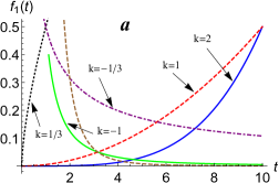
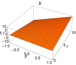
Figure 1: Fig (a) shows the variation of $f_{1}(t)$ with $t$ for different values of $k$. The initial condition is fixed at $\alpha=0.5$. Fig (b) shows the variation of $f_{2}(t)$ with $t$ and $\beta$.

A black hole will be formed if we obtain only non-positive solution of this equation. However, if we obtain a positive real root for this equation, then this system will be described by a naked singularity. Here it is difficult to find exact solutions for $X_{0}$ except for some particular values. This is because the governing equation of the system is a very complicated one. These exact solutions are given in the following Table 1. It is clear from the table that certain conditions between the parameters are required to be satisfied in order to make the solutions positive.

$k$	$Regime$	$Solution1$	$Solution2$
$0$	$Dust$	$\frac{U-\alpha-\sqrt{\left(U-\alpha\right)^{2}-8\beta}}{2\beta}$	$\frac{U-\alpha+\sqrt{\left(U-\alpha\right)^{2}-8\beta}}{2\beta}$
$1$	$stiff~{}fluid$	$\frac{\beta}{3\alpha}+\frac{2^{1/3}Y}{3\alpha\left(Z+\sqrt{4Y^{3}+Z^{2}}\right)^{1/3}}-\frac{\left(Z+\sqrt{4Y^{3}+Z^{2}}\right)^{1/3}}{3\times 2^{1/3}\alpha}$	$-$
$-1/2$	$DE$	$\frac{U-\sqrt{U^{2}-2\beta\left(\alpha+4\right)}}{2\beta}$	$\frac{U+\sqrt{U^{2}-2\beta\left(\alpha+4\right)}}{2\beta}$

Table 1: Exact Values of $X_{0}$ for specific values of the EoS parameter $k$ obtained from Eq.(3.25) where 
                     $U=1+c^{2}c_{2}\mathcal{M}^{2}$,

                     $Y=3\alpha+3c^{2}c_{2}\mathcal{M}^{2}\alpha-\beta^{2}$,

                     $Z=-54\alpha^{2}+9\alpha\beta+9c^{2}c_{2}\mathcal{M}^{2}\alpha\beta-2\beta^{3}$.

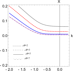
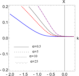
Figure 2: Figs (a) and (b) show the variation of $X_{0}$ with $k$ for different values of $\mathcal{M}$ and $\alpha$ respectively. In Fig(a) the initial conditions are fixed at $\alpha=0.5$, $\beta=2$, $c=2$, $c_{2}=2$. In Fig.(b) the initial conditions are fixed at $\mathcal{M}=5$, $\beta=2$, $c=2$, $c_{2}=2$.

We now analyze the results furnished in the Table 1.

Case 1: k=0

This corresponds to the pressureless dust regime of the universe. For the solutions to be real and finite, we must have $\beta\neq 0$, $\left(U-\alpha\right)^{2}\geq 8\beta$.
For positivity of the first solution we have for $\beta>0$,  $U-\alpha\geq\sqrt{\left(U-\alpha\right)^{2}-8\beta}\Longrightarrow\beta\geq 0$. But since $\beta\neq 0$, we must restrict ourselves to $\beta>0$, which is in agreement with our assumption. So the first solution is positive for any positive $\beta$. For $\beta<0$, we have for positive solution $U-\alpha\leq\sqrt{\left(U-\alpha\right)^{2}-8\beta}\Longrightarrow\beta\leq 0$. But since $\beta\neq 0$, we must have $\beta<0$ which is in agreement with our assumption. So, for $\beta<0$, the solution 1 is always positive and represents a NS. Hence, for any non-zero real $\beta$ the first solution represents an NS.
For solution 2 to be positive we must have for $\beta>0$, $U-\alpha\geq-\sqrt{\left(U-\alpha\right)^{2}-8\beta}\Longrightarrow\beta\geq 0$. This gives $\beta>0$, just like the previous case. Hence, the solution is positive. Similarly for $\beta<0$ case also we get positive solution. Thus, this solution also represents NS. Therefore for $k=0$, we get NS as the end state of collapse.

Case 2: k=1

This corresponds to the early stiff fluid era of our universe. Here, the situation is much more chaotic mathematically. We get only one solution, which turns out to be a relatively complicated one. Now physically speaking, in the early universe, due to big bang extreme amount of chaos is expected. Moreover, there are quantum fluctuations, so mathematically the scenario is justified. Here, in order to have a positive solution we should have $\frac{\beta}{3\alpha}+\frac{2^{1/3}Y}{3\alpha\left(Z+\sqrt{4Y^{3}+Z^{2}}\right)^{1/3}}\geq\frac{\left(Z+\sqrt{4Y^{3}+Z^{2}}\right)^{1/3}}{3\times 2^{1/3}\alpha}$. Moreover for negative $Y$, $Z^{2}\geq 4Y^{3}$ for the solution to be real.

Case 3: k=-1/2

This represents the dark energy era corresponding to the late time accelerated expanding universe. Here, the solution to be real and finite we have, $\beta\neq 0$, $U^{2}\geq 2\beta\left(\alpha+4\right)$. For positive solution, we must have $\beta\left(\alpha+4\right)\geq 0$ in which for $\beta>0$ $\Longrightarrow$ $\alpha\geq-4$. For $\beta<0$, we should have $\beta\left(\alpha+4\right)\leq 0$ $\Longrightarrow$ $\alpha\leq-4$ in order to get a positive solution.

Numerical Solutions of $X_{0}$ and their interpretations

In order to understand the dynamics of collapse, we need to have a knowledge of $X_{0}$ not at discrete points of $k$, but throughout the cosmologically meaningful region $k<1$, i.e., from early to late universe. To achieve this we proceed to obtain numerical solutions of $X_{0}$, by assigning different initial conditions to the parameters describing this system. To visualize these solutions we obtain contours for $k-X_{0}$ for different numerical values of the involved parameters.

It may be noted from the plots that the trajectories run across the positive range of $X_{0}$ thus confirming the formation of NS. In Fig.2(a), we can observe the dependence of $X_{0}$ on the EoS parameter $k$ for different values of the massive gravity parameter $\mathcal{M}$. We see that an increase in the value of $\mathcal{M}$ decreases the tendency of formation of NS. Hence we observe that the dynamics of the system gets deformed by the addition of graviton mass to this system. In Fig.2(b), the $k-X_{0}$ trajectories for different values of $\alpha$ are obtained. Here also different values of $\alpha$ deform the dynamics of this system. Greater the value of $\alpha$, greater is the tendency to form NS.

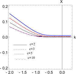
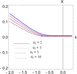
Figure 3: Figs (a) and (b) show the variation of $X_{0}$ with $k$ for different values of $c$ and $c_{2}$ respectively.In Fig.3(a) the initial conditions are fixed at $\alpha=0.5$, $\beta=2$, $c_{2}=2$, $\mathcal{M}=5$. In Fig.3(b) the initial conditions are taken as $\alpha=0.5$, $\beta=2$, $c=2$, $\mathcal{M}=5$.

In Fig.3(a), we observe the effect of $c$ on the collapsing system. It is observed that greater the value of $c$, lesser is the tendency to form NS. In Fig.3(b), we can observe the effect of $c_{2}$ on the system. Here also we see that an increase in $c_{2}$ decreases the possibility of NS.

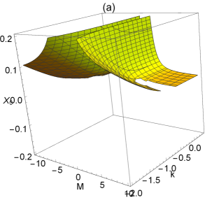
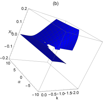
Figure 4: Fig (a) shows the variation of $X_{0}$ with $k$ and $\mathcal{M}$. The initial conditions are fixed at $\alpha=0.5,\beta=2$, $c=2$, $c_{2}=2$. Fig (b) shows the variation of $X_{0}$ with $k$ and $\alpha$. The initial conditions are taken as $\mathcal{M}=5,\beta=2$, $c=2$, $c_{2}=2$.

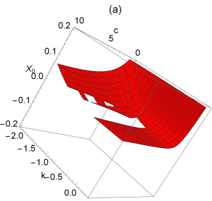
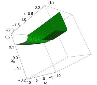
Figure 5: Fig (a) shows the variation of $X_{0}$ with $k$ and $c$. The initial conditions are fixed at $\alpha=0.5,\beta=2$, $\mathcal{M}=5$, $c_{2}=2$. Fig (b) shows the variation of $X_{0}$ with $k$ and $c_{2}$. The initial conditions are taken as $\alpha=0.5,\beta=2$, $\mathcal{M}=5$, $c=2$.

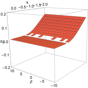
Figure 6: Fig 6 shows the variation of $X_{0}$ with $k$ and $\beta$. The initial conditions are fixed at $\mathcal{M}=5$, $c=2$, $c_{2}=2$, $\alpha=0.5$.

In Figs.4, 5 and 6, 3D-plots are obtained to get a more comprehensive view of the dynamics of the collapse. In all the figures the resulting surfaces entirely lie in the positive half-space of $X_{0}$, thus showing the presence of NS. In Fig.4(a), the variation of $k-\mathcal{M}$ surfaces are obtained against $X_{0}$. We see that in the dark energy regime $(k<-1/3)$ the surface pushes towards the positive direction of $X_{0}$, accompanied with a decrease in $\mathcal{M}$, thus showing an increased tendency to form NS. In Fig.4(b), $k-\alpha$ surfaces are obtained against $X_{0}$. Here also in the dark energy regime, there is an increased tendency of NS accompanied by an increase in $\alpha$. In Fig.5(a), $k-c$ surface is obtained against $X_{0}$. Here accompanied by a decrease in the value of $c$, we witness an increased tendency of NS in the dark energy regime. In Fig.5(b), $k-c_{2}$ surface is obtained against $X_{0}$. The results obtained are same as that of Fig.5(a). In Fig.6, $k-\beta$ surface is obtained against $X_{0}$. We see that the $k-\beta$ surface is parallel to the $\beta$ axis. This shows that the system is not deformed by $\beta$ and hence the collapse dynamics does not depend on it. This is an important result. Finally just like the previous cases here also the surface gets lifted in the dark energy regime towards the positive direction of $X_{0}$ axis.

Strength of Singularity

It is important to know about the destructive capacity of a singularity, and this is measured using the concept of strength of singularity. The strength of singularity is related to the extension of spacetime through the singularity. Now this can be quantified using the Tipler’s formalism [74]-[77]. Now using the Tipler’s formalism [74]-[77], the condition for a singularity to be strong is given by,

$$\begin{array}[]{c}S=lim~{}~{}\tau^{2}\psi\\ \tiny\tau\rightarrow 0\\ \end{array}\begin{array}[]{c}=lim~{}~{}\tau^{2}R_{\mu\nu}K^{\mu}K^{\nu}>0\\ \tiny\tau\rightarrow 0\\ \end{array}$$ (3.30)

where $R_{\mu\nu}$ is the Ricci tensor. Here $\psi$ is a scalar given by $\psi=R_{\mu\nu}K^{\mu}K^{\nu}$, $K^{\mu}=\frac{dx^{\mu}}{d\tau}$ is the tangent to the non-spacelike geodesics at the singularity, and $\tau$ is the affine parameter. It has been demonstrated that [77],

$$\begin{array}[]{c}S=lim~{}~{}\tau^{2}\psi\\ \tiny\tau\rightarrow 0\\ \end{array}\begin{array}[]{c}=\frac{1}{4}X_{0}^{2}\left(2\dot{m_{0}}\right)\\ {}\tiny\hfil\\ \end{array}$$ (3.35)

where $m_{0}$ is given by

$$\begin{array}[]{c}m_{0}=lim~{}~{}m(t,r)\\ \tiny t\rightarrow 0\\ \tiny r\rightarrow 0.\end{array}$$ (3.39)

Furthermore, it is also possible to write

$$\begin{array}[]{c}\dot{m_{0}}=lim~{}~{}\frac{\partial}{\partial~{}t}\left(m(t,r)\right)\\ \tiny t\rightarrow 0\\ \tiny r\rightarrow 0.\end{array}$$ (3.43)

Using Eq. (3.2) in the above relation (3.35), we obtain

$$\begin{array}[]{c}S=lim~{}~{}\tau^{2}\psi\\ \tiny\tau\rightarrow 0\\ \end{array}\begin{array}[]{c}=\frac{1}{4}X_{0}^{2}\left[\frac{2k\alpha}{1-2k}X_{0}^{2k-1}+\beta\right]\\ {}\tiny\hfil\\ \end{array}$$ (3.48)

It may be noted that it has been demonstrated that $X_{0}$ is related to the limiting values of mass as [77]

$$X_{0}=\frac{2}{1-2m_{0}^{\prime}-2\dot{m_{0}}X_{0}}$$ (3.49)

where $m_{0}^{\prime}$ is given by

$$\begin{array}[]{c}m_{0}^{\prime}=lim~{}~{}\frac{\partial}{\partial~{}r}\left(m(t,r)\right)\\ \tiny t\rightarrow 0\\ \tiny r\rightarrow 0.\end{array}$$ (3.53)

Here $\dot{m_{0}}$ is given by the Eq. (3.43). Now using Eqs. (3.2), (3.43) and (3.53) in Eq. (3.49), we obtain

$$\frac{2\alpha}{1-2k}X_{0}^{2k+1}+2\beta X_{0}^{2}-\left(1+2\mathcal{M}^{2}c^{2}c_{2}\right)X_{0}-2=0$$ (3.54)

In a particular case, if $k=-1/2$ (dark energy) is considered, we obtain a solution for Eq. (3.54) as

$$X_{0}=\frac{0.25}{\beta}\left(1+2c^{2}c_{2}\mathcal{M}^{2}+\sqrt{8\beta\left(2-\alpha\right)+\left(1+2c^{2}c_{2}\mathcal{M}^{2}\right)^{2}}\right)$$ (3.55)

which is positive when  $1+2c^{2}c_{2}\mathcal{M}^{2}\geq 2\sqrt{2\beta\left(\alpha-2\right)}$ and $\alpha>2$ for $\beta>0$, provided $c_{2}>0$. The existence of such a positive root signifies that the singularity is naked. Using the above value of $X_{0}$ in the Eq. (3.63), we get

$$\begin{array}[]{c}S=lim~{}~{}\tau^{2}\psi\\ \tiny\tau\rightarrow 0\\ \end{array}\begin{array}[]{c}=\frac{0.03125}{\beta}u^{2}\left(1-\frac{8\alpha\beta}{u^{2}}\right)\\ {}\tiny\hfil\\ \end{array}$$ (3.60)

where we have $u=1+2c^{2}c_{2}\mathcal{M}^{2}+\sqrt{8\beta\left(2-\alpha\right)+\left(1+2c^{2}c_{2}\mathcal{M}^{2}\right)^{2}}$.
Here, we can write

$$\begin{array}[]{c}S=lim~{}~{}\tau^{2}\psi>0\\ \tiny\tau\rightarrow 0\\ \end{array}$$ (3.63)

for $8\alpha\beta<u^{2}$ for $\beta>0$. This is the condition for a strong naked singularity. A $3D$ plot for $S$ is shown in Fig.7 for a particular scenario. The plot shows that the surface lies in the positive region thus giving a strong naked singularity.

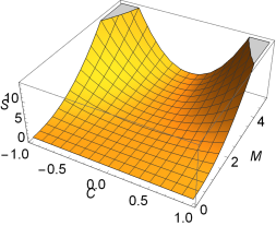
Figure 7: The figure shows the variation of $S$ with $c$ and $\mathcal{M}$. The initial conditions are fixed at $\beta=2$, $c_{2}=2$, $\alpha=0.5$.

4 Thermodynamics

In this section, we would like to study the thermodynamics of generalized Vaidya spacetime in massive gravity. The thermalization temperature, for such a spacetime, is given by the following relation [51],

$$T=\frac{1}{4\pi}\frac{d}{dr}f(t,r)|_{r=r_{h}},$$ (4.1)

where $r_{h}$ is the event horizon obtained from the following relation (see the equation (3.3)),

$$-1+\frac{r^{-2k}}{1-2k}f_{1}(t)+\frac{f_{2}(t)}{r}-\frac{1}{2}\mathcal{M}^{2}cc_{1}r-\mathcal{M}^{2}c^{2}c_{2}=0.$$ (4.2)

Real positive root of the above equation gives the event horizon radius. In Fig.8, we can see the typical behavior of $f(t,r)$ in terms of $r$. We show that it is possible to have two radii at which $f(t,r)=0$, and the bigger one (solid red) shows the event horizon radius (about $r=4$ of Fig.8). We can also see that the increasing value of $k$ increases the value of outer event horizon radius. In the case of $k>0.5$ we can see only one zero (see red and blue lines). Also, we can see extremal case with $k=-2$ and $\mathcal{M}=0.287$. We should note that having one or two horizons is a function of the massive parameter $\mathcal{M}$.

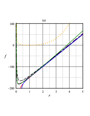
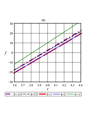
Figure 8: Horizon structure of the generalized Vaidya spacetime in massive gravity. It is set $f_{1}(t)=f_{2}(t)=c=c_{1}=c_{2}=2$ and $\mathcal{M}=5$ and the dotted orange line in plot (a) represents $k=-2$ and $\mathcal{M}=0.5$. Plot (b) shows the zoomed range of outer horizon given by the plot (a).

In the special case of $k=-1$, one can obtain real positive root as,

$$r_{h}=\frac{1}{2f_{1}}\left(Y^{\frac{1}{3}}+\frac{c_{1}^{2}c^{2}\mathcal{M}^{4}+4f_{1}(c_{2}c^{2}\mathcal{M}^{2}+1)}{Y^{\frac{1}{3}}}-c_{1}c\mathcal{M}^{2}\right),$$ (4.3)

where we defined,

$$Y=2\sqrt{3}f_{1}\sqrt{M}-12f_{2}{f_{1}}^{2}-6\left(c_{2}{c}^{2}{\mathcal{M}}^{2}+1\right){\mathcal{M}}^{2}c_{1}cf_{1}-{\mathcal{M}}^{6}{c_{1}}^{3}{c}^{3},$$ (4.4)

where

$$M = -3{c_{1}}^{2}{c_{2}}^{2}{c}^{6}{\mathcal{M}}^{8}+\left(-16\,f_{1}{c_{2}}^{3}{c}^{6}+6f_{2}{c_{1}}^{3}{c}^{3}-6{c_{1}}^{2}c_{2}{c}^{4}\right){\mathcal{M}}^{6}$$ (4.5)

$$+ \left(36\,f_{1}f_{2}c_{1}c_{2}{c}^{3}-48\,f_{1}{c_{2}}^{2}{c}^{4}-3{c_{1}}^{2}{c}^{2}\right){\mathcal{M}}^{4}$$

$$+ 36\,f_{1}c\left(f_{2}c_{1}-\frac{4}{3}c_{2}c\right){\mathcal{M}}^{2}+36{f_{1}}^{2}{f_{2}}^{2}-16\,f_{1}.$$

By using the equation (4.1) one can obtain,

$$T=\frac{1}{4\pi}\left(\frac{{\mathcal{M}}^{2}}{2c_{1}c}-\frac{2kf_{1}}{1-2k}r_{h}^{-2k-1}-f_{2}r_{h}^{-2}\right).$$ (4.6)

In the plots of the Fig.9 we can see typical behavior of the temperature for some values of $k$ in terms of $r$ (a) and in terms of $\mathcal{M}$ (b). Fig.9 (a) plotted in terms of $r$, however from the Figs.8 we show that selected value of parameters yields $r_{h}\approx 4$. Instead of small radius, in the special case of $k=-1$, it is approximately linear function of radius. We can see that for the case of $k<0.5$, temperature is increasing function of $r$ to yields a constant for the large radius. Situation is vise for the cases of $k>0.5$ (see red and blue solid lines).
Then, by using the relation (4.3) one can obtain temperature in terms of $\mathcal{M}$ in which we can find it as increasing function of $\mathcal{M}$. Also, we can see that increasing $\beta$ ($f_{2}$) decreases the temperature.

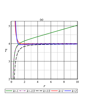
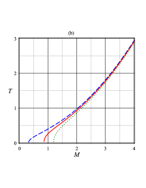
Figure 9: Typical behavior of the temperature. (a) in terms of radius; (b) in terms of $\mathcal{M}$ for $f_{1}(t)=2$ and $f_{2}(t)=1,5,9$ respectively denoted by dashed blue, solid red and dotted green lines. $c=c_{1}=c_{2}=2$, and $\mathcal{M}=5$, and $k=-1$.

Now, we can write entropy as,

$$S=\pi^{2}r_{h}^{2},$$ (4.7)

where we used $\pi G=1$. Hence, we can use the following relation to calculate total energy,

$$U=\int{TdS},$$ (4.8)

which yields to the following expression,

$$U=-\frac{1}{2}\,\pi\,f_{2}\ln\left(r_{h}\right)+\frac{1}{8}{\mathcal{M}}^{2}\pi\,c_{1}c{r_{h}}^{2}-\frac{\pi kf_{1}}{4k^{2}-4k+1}r_{h}^{1-2k}.$$ (4.9)

In the Fig.10 (a) we can see typical behavior of $U$ for some values of $k$ and find that value of $k$ reduces value of the internal energy. Also, in the Fig.10 (b) we can see that internal energy is increasing function of mass parameter. Internal energy may be used to obtain Helmholtz free energy.

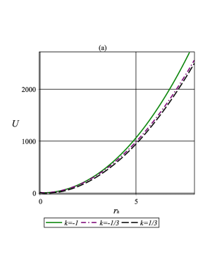
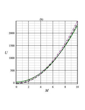
Figure 10: Typical behavior of the internal energy in terms of (a) radius with $\mathcal{M}=5$ and (b) mass parameter $\mathcal{M}$ with $r_{h}\approx 4$ for $f_{1}(t)=f_{2}(t)=c=c_{1}=c_{2}=2$.

Helmholtz free energy can be obtained via the following relation,

$$F=U-TS,$$ (4.10)

which yields to the following expression,

$$F=\frac{kf_{1}r_{h}^{1-2k}+\sqrt{k-\frac{1}{2}}\left[kf_{1}r_{h}^{1-2k}+2f_{2}(k-\frac{1}{2})(\ln{r_{h}}-\frac{1}{2})\right]}{-\frac{4}{\pi}\sqrt{k-\frac{1}{2}}}.$$ (4.11)

It is interesting to note that Helmholtz free energy is independent of $\mathcal{M}$. In the plots of the Fig.11, we can see typical behavior of the Helmholtz free energy in terms of radius for various values of $k$.

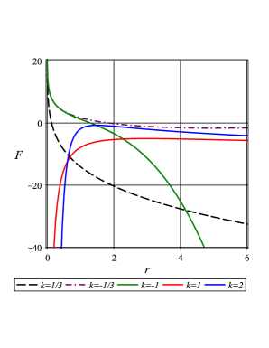
Figure 11: Typical behavior of the Helmholtz free energy in terms of radius for $f_{1}(t)=f_{2}(t)=c=c_{1}=c_{2}=2$.

Finally, we can study specific heat in constant volume,

$$C=\left(\frac{dU}{dT}\right)_{V},$$ (4.12)

which yields to the following expression,

$$C=\pi r_{h}^{2}\frac{kf_{1}r_{h}^{1-2k}-(f_{2}-\frac{1}{2}\mathcal{M}^{2}c_{1}cr_{h}^{2})(k-\frac{1}{2})}{f_{2}(k-\frac{1}{2})-kf_{1}(k+\frac{1}{2})r_{h}^{1-2k}},$$ (4.13)

In the plots of the Fig.12 we can see typical behavior of the specific heat in terms of the mass parameter and radius. We can see that specific heat may be positive or negative (for $k$ of order unit) which means some instability with possible phase transition. One can study such instability in the context of thermal fluctuations [78, 79, 80, 81, 82, 83] and find that presence of thermal fluctuations may remove mentioned instabilities. Also, Fig.12 (b) shows that specific heat is increasing function of mass parameter.

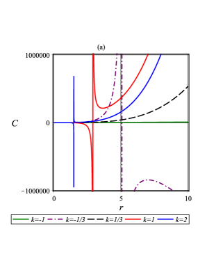
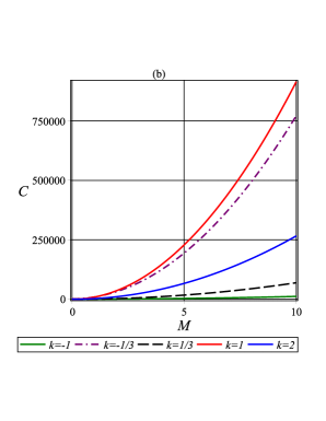
Figure 12: Typical behavior of the specific heat in terms of (a) radius with $\mathcal{M}=5$ and (b) mass parameter $\mathcal{M}$ with $r_{h}=4$ for $f_{1}(t)=f_{2}(t)=c=c_{1}=c_{2}=2$.

5 Conclusions and Discussion

In this paper, we have analyzed the gravitational collapse in massive gravity. It was observed that the dynamics of this system are changed due to the addition of a mass to this system. In this paper, we first obtained equation of motion for a time dependent solution in massive gravity. Then barotropic equation of state was used to further analyze such solutions. Finally, we applied this solution to a dynamics of gravitational collapse. It was observed that the gravitational collapse depends on the value of the mass used to deform this theory.

Contours for $X_{0}$ are obtained against the barometric parameter $k$ for different values of other parameters like $\mathcal{M}$, $\alpha$, $\beta$, etc. Various regimes of the fluid content of the universe has been plotted such as radiation ($k>0$), pressure-less dust ($k=0$), dark energy ($k<0$), phantom ($k<-1$). From the figures we see that there is no trajectories in the negative region. This rules out the existence of black holes as the end state of collapse in the context of massive gravity with the considered parameters.

From the first Figs.2, 3, 4, 5, 6, we see that the contours and surfaces of $X_{0}$ obtained against the parameters $\mathcal{M}$, $\alpha$, $\beta$ and $k$ lie in the positive region. This confirms the existence of positive roots of equation (3.25) and indicates the end state of the collapse can be a naked singularity in the context of massive gravity with the considered parameters.

In Fig.2(a), we see that an increase in the value of massive gravity parameter $\mathcal{M}$ decreases the tendency of formation of NS. Hence, we observe that the dynamics of the system gets deformed by the addition of graviton mass to this system. In Fig.2(b), the $k-X_{0}$ trajectories for different values of $\alpha$ are obtained and represents that greater values of $\alpha$ increase the tendency to form NS. In contrast, in Figs.3(a) and 3(b), we observe that greater values of $c$ and $c_{2}$ decrease the tendency to form the NSs. In Fig.4(a), the variation of $k-\mathcal{M}$ surfaces are obtained against $X_{0}$. We see that in the dark energy regime $(k<-1/3)$ the surface pushes towards the positive direction of $X_{0}$, accompanied with a decrease in $\mathcal{M}$, thus showing an increased tendency to form NS. In Fig.4(b), $k-\alpha$ surfaces are obtained against $X_{0}$. Here also in the dark energy regime, there is an increased tendency of NS accompanied by an increase in $\alpha$. In Fig.5(a), $k-c$ surface is obtained against $X_{0}$. Here accompanied by a decrease in the value of $c$, we witness an increased tendency of NS in the dark energy regime. In Fig.5(b), $k-c_{2}$ surface is obtained against $X_{0}$. The results obtained are same as that of Fig.5(a). In Fig.6, we see that the $k-\beta$ surface is parallel to the $\beta$ axis around $k=0$ and this shows that the system is not deformed by $\beta$ and hence the collapse dynamics does not depend on it in the early universe regime. But what matters is that the surface remains totally in the $X_{0}>0$ region. Eventually the surface pushes up towards the positive axis for $k\leq-0.5$, i.e. in the dark energy regime. This shows an increased tendency to form naked singularities. In the figs. 4-6, we see that the surfaces totally lie in the $X_{0}>0$ region thus showing the possibility of formation of naked singularities. We have also studied the strength of the singularity formed and showed that under certain conditions, and concluded that strong singularities are possible in massive gravity. This is illustrated in Fig.7. It would be interesting to analyze the strength of such naked singularities, for various models, and compare the results of massive gravity with general relativity.

From the above discussion, we conclude that this work provides counterexamples of the cosmic censorship conjuncture, which states that every singularity must be covered by an event horizon, in the context of massive gravity. We would like to point out that there are two forms of the cosmic censorship conjuncture [84]-[85]. According to the strong cosmic censorship conjuncture, no locally naked singularities can occur. However, according to the weak cosmic censorship conjuncture, singularities can be locally naked, but they cannot be globally naked. It is also possible to analyze the strength of singularities, and this can be done using the Tipler’s formalism [74]-[77]. We have applied this formalism to the massive gravity, and demonstrated that it possible to have a strong naked singularity in massive gravity.

Finally, we study thermodynamics of the model and calculate some thermodynamical quantities to investigate effect of mass parameter. For example, in Figs.9(b) and 12(b), we find that the thermalization temperature and specific heat respectively are increasing function of $\mathcal{M}$. We also found some instabilities, corresponding to special values of $k$, and we found stable/unstable black hole phase transition. For the future work we would like to focus on the instabilities and consider effect of thermal fluctuations to see that what can happen with the instable regions.

References

- [1] A.G. Riess et al., Astron. J. 116, 1009 (1998)
- [2] S. Perlmutter et al., Nature 391 , 51 (1998)
- [3] A. G. Riess et al., Astron. J. 118, 2668 (1999)
- [4] S. Perlmutter et al., Astrophys. J. 517, 565 (1999)
- [5] A. G. Riess et al., Astrophys. J. 560, 49 (2001)
- [6] J. L. Tonry et al., Astrophys. J. 594, 1 (2003)
- [7] P. J. E. Peebles, and B. Ratra, Rev. Mod. Phys.75, 559 (2003)
- [8] E. J. Copeland, M. Sami, and S. Tsujikawa, Int. J. Mod. Phys.D15, 1753 (2006)
- [9] J. A. Frieman, M. S. Turner, and D. Huterer, Annual Review of Astronomy and Astrophysics, 46, 385 (2008)
- [10] M. Khurshudyan, B. Pourhassan, A. Pasqua, Can. J. Phys. 93 (2015) 449
- [11] H. van Dam and M. J. G. Veltman, Nucl. Phys. B 22, 397 (1970)
- [12] Y. Iwasaki, Phys. Rev. D 2, 2255 (1970)
- [13] S. Upadhyay, B. Pourhassan, H. Farahani, Phys. Rev. D 95, 106014 (2017)
- [14] W. Pauli and M. Fierz Helv. Phys. Acta 12, 297 (1939)
- [15] M. Fierz Helv. Phys. Acta 12, 3 (1939)
- [16] A. I. Vainshtein, Phys. Lett. B 39, 393 (1972)
- [17] E. Babichev and C. De ayet, Class. Quant. Grav. 30, 184001 (2013)
- [18] D. G. Boulware, S. Deser, Phys. Rev. D 6, 3368 (1972)
- [19] de Rham C, Gabadadze G and Tolley A J 2011 Phys. Rev. Lett. 106, 231101 (2011)
- [20] de Rham C and Gabadadze G Phys. Rev. D 82, 04402 (2010)
- [21] de Rham C, Gabadadze G and Tolley A J Phys. Lett. B 711, 190 (2012)
- [22] S. F. Hassan, R. A. Rosen and A. Schmidt-May, JHEP 1202, 026 (2012)
- [23] S. F. Hassan, A. Schmidt-May and M. von Strauss, Phys. Lett. B 715, 335 (2012)
- [24] S. F. Hassan and R. A. Rosen Phys. Rev. Lett. 108, 041101 (2012)
- [25] S. F. Hassan S F and R. A. Rosen JHEP 1204, 123 (2012)
- [26] K. Hinterbichler, Rev. Mod. Phys. 84, 671 (2012)
- [27] A. H. Chamseddine and V. Mukhanov, JHEP 1208, 036 (2012)
- [28] I. Arraut, arXiv:1505.06215 [gr-qc].
- [29] S. Dengiz, arXiv:1409.5371 [hep-th]
- [30] G. Goon, K. Hinterbichler, A. Joyce and M. Trodden, JHEP 1507, 101 (2015)
- [31] S. H. Hendi, S. Panahiyan, B. E. Panah, JHEP 01, 129 (2016)
- [32] Se. H. Hendi, G. Q. Li, J. X. Mo, S. Panahiyan and B. E. Panah, Eur. Phys. J. C 76, 571 (2016)
- [33] S. H. Hendi, S. Panahiyan, B. E. Panah and M. Momennia, Ann. der Phys. 528, 819 (2016)
- [34] M. Wyman, W. Hu and P. Gratia, Phys. Rev. D 87, 084046 (2013)
- [35] M. S. Volkov, Phys.Rev. D 90, 024028 (2014)
- [36] A. Sinha, JHEP 1006, 061 (2010)
- [37] J. Sadeghi and B. Pourhassan, JHEP12 (2008) 026
- [38] B. Pourhassan and J. Sadeghi, Can J Phys 91 (2013) 995
- [39] J. Sadeghi, B. Pourhassan and S. Heshmatian, Advances in High Energy Physics 2013 (2013) 759804
- [40] V. Niarchos, Fortsch. Phys. 57, 646 (2009)
- [41] X. X. Zeng, H. Zhang and L. F. Li, Phys. Lett. B 756, 170 (2016)
- [42] W. J. Pan and Y. C. Huang, arXiv:1612.03627
- [43] L. Alberte and A. Khmelnitsky, Phys. Rev. D 91, 046006 (2015)
- [44] V. Ziogas, JHEP 09, 114 (2015)
- [45] V. Keranen and P. Kleinert, Phys. Rev. D 94, 026010 (2016)
- [46] P. C. Vaidya, Curr. Sci. 12, 183 (1943)
- [47] P. C. Vaidya, Nature 171, 260 (1953)
- [48] P. Li, X. Z. Li and X. H. Zhai, Phys. Rev. D 94, 124022 (2016)
- [49] Y. P. Hu, X. X. Zeng and H. Q. Zhang, Phys. Lett. B 765, 120 (2017)
- [50] K. B. Fadafan, B. Pourhassan and J. Sadeghi, Eur. Phys. J. C 71, 1785 (2011)
- [51] E. Caceres, A. Kundu and D. L. Yang, JHEP 1403, 073 (2014)
- [52] M. Sharif and A. Siddiqa, Gen. Rel. Grav. 43, 73 (2011)
- [53] M. Sharif and A. Siddiqa, Mod. Phys. Lett. A 25, 2831 (2010)
- [54] P. Rudra, R. Biswas, U. Debnath, Astrophys. Space Sci. 335, 505 (2011)
- [55] U. Debnath, P. Rudra, R. Biswas, Astrophys. Space Sci. 339, 135 (2012)
- [56] P. Rudra, R. Biswas, U. Debnath, Astrophys. Space Sci. 354, 597 (2014)
- [57] P. Rudra, U. Debnath, Can. J. Phys. 92(11), 1474 (2014)
- [58] P. Rudra, M. Faizal, A. F. Ali, Nucl. Phys. B. 909, 725 (2016)
- [59] Y. Heydarzade, P. Rudra, F. Darabi, A. F. Ali, M. Faizal, Phys. Lett. B. 774, 46 (2017)
- [60] I. H. Dwivedi and P. S. Joshi, Class. Quant. Grav. 6, 1599 (1989)
- [61] I. H. Dwivedi and P. S. Joshi, Class. Quant. Grav. 8, 1339 (1991)
- [62] I. H. Dwivedi and P. S. Joshi, J. Math. Phys. 32, 2167 (1991)
- [63] I. H. Dwivedi and P. S. Joshi, Phys. Rev. D 45, 2147 (1992)
- [64] K. Lake, Phys. Rev. D 43, 1416 (1991)
- [65] S. M. Wagh and S. D. Maharaj, Gen. Rel. Grav. 31, 975 (1999)
- [66] S. G. Ghosh and A. Beesham, Phys. Rev. D 61, 067502 (2000)
- [67] S. G. Ghosh and N. Dadhich,, Phys. Rev. D 64, 047501 (2001)
- [68] A. Beesham and S. G. Ghosh, Int. J. Mod. Phys. D12, 801 (2003)
- [69] R. G. Cai, Y. P. Hu, Q. Y. Pan and Y. L. Zhang, Phys. Rev. D 91 024032 (2015)
- [70] D. M. Eardley, and L. Smar , Phys. Rev. D 19, 2239 (1979)
- [71] P. S. Joshi, I. H. Dwivedi, Commun. Math. Phys. 146, 333 (1992)
- [72] P. S. Joshi, T. P. Singh, Phys. Rev. D 51, 6778 (1995)
- [73] T. P. Singh, P. S. Joshi, Class. Quant. Grav. 13, 559 (1996)
- [74] F. J. Tipler, Phys. Lett. A. 64, 8 (1977)
- [75] V. D. Vertogradov, J Phys. Conf. Series, 769, 012013 (2016)
- [76] V.D. Vertogradov, Grav. Cosmol. 22, 220 (2016)
- [77] M. D. Mkenyeleye, R. Goswami, and S. D. Maharaj, Phys. Rev. D 90, 064034 (2014)
- [78] B. Pourhassan and M. Faizal, Nucl. Phys. B 913, 834 (2016)
- [79] J. Sadeghi, B. Pourhassan and M. Rostami, Phys. Rev. D 94, 064006 (2016)
- [80] B. Pourhassan and M. Faizal, Phys. Lett. B 755, 444 (2016)
- [81] B. Pourhassan, M. Faizal and U. Debnath, Eur. Phys. J. C 76, 145 (2016)
- [82] M. Faizal and B. Pourhassan, Phys. Lett. B 751, 487 (2015)
- [83] B. Pourhassan and M. Faizal, Europhys. Lett. 111, 40006 (2015)
- [84] T. P. Singh, gr-qc/9606016
- [85] S. S. Deshingkar, S. Jhingan and P. S. Joshi, Gen. Rel. Grav. 30, 1477 (1998)