Generalization of Taylor’s formula to particles of arbitrary inertia

Abstract

One of the cornerstones of turbulent dispersion is the celebrated Taylor formula. This formula expresses the rate of transport (i.e. the eddy diffusivity) of a tracer as a time integral of the fluid velocity auto-correlation function evaluated along the fluid trajectories. Here, we review the hypotheses which permit to extend Taylor’s formula to particles of any inertia. The hypotheses are independent of the details of the inertial particle model. We also show by explicit calculation, that the hypotheses encompass cases when memory terms such as Basset and the Faxén corrections are taken into account in the modeling of inertial particle dynamics.

I Introduction

In the early 20s of last century Sir Geoffrey Ingram Taylor derived what can be fairly considered one of the cornerstones of large-scale transport of tracer particles in fluid flows Tay22 . Tracer particles are small particles not affecting the advecting velocity field with their motion:

$$\frac{d\bm{x}}{dt}=\bm{u}(\bm{x},t)$$ (1)

In the the limit of long observation time and in suitable conditions, Taylor observed that the mean square of tracer particles displacement behaved linearly in time with a coefficient now usually referred to as the eddy-diffusivity coefficient ( see e.g. BiCrVeVu95 ; Frisch ; Maz1997 ; MaMuVu05 ; CeMaMuVu06 ; BoMaLa16 ):

$$\left\langle||\bm{x}(t)-\langle\bm{x}(t)\rangle||^{2}\right\rangle\sim 2Dt$$ (2)

Based on this observation, Taylor proceeded to establish a first principle identity expressing the tracer particle eddy diffusivity as a time integral of the fluid velocity auto-correlation function evaluated along the fluid trajectories:

$$D=\lim_{t\to\infty}\int_{0}^{t}ds\left\langle\delta\bm{u}(\bm{x}(t),t)\cdot\delta\bm{u}(\bm{x}(s),s)\right\rangle$$ (3)

where $\delta\bm{u}(\bm{x}(t),t)=\bm{u}(\bm{x}(t),t)-\langle\bm{u}(\bm{x}(t),t)\rangle$.

Since then, the relation (3) now going under the name of Taylor’s formula has played a key role in the analysis of turbulent dispersion of tracers Kra87 ; MK99 . We refer e.g. to chapter 12 of the textbook KuCoDo12 for a review including an introduction to the vast existing literature.

Tracer dispersion is a small sub-set of a much larger class of transport problems: the transport of inertial particles. Inertial particles are small particles having a finite size and/or different density from that of the carrier fluid where they are suspended ToBo09 . Inertial particles are encountered practically everywhere, from our atmosphere (e.g., affecting the Earth’s climate system because of its effect on global radiative budget by scattering and absorbing long-wave and short-wave radiation IPCC ; or leading to increased droplet collisions and the formation of larger droplets with a key role for rain initiation FFS01 ; Mazz1 ; Mazz2 ) and ocean (e.g. in relation to phytoplankton dynamics in turbulent ocean FL2015 ) to astrophysics (in relation to planet formation e.g. BrChPrSp99 ; WiMeUs08 ).

It is therefore not surprising that deriving extensions of Taylor’s formula to inertial particle dynamics has stirred interest for now already half a century Tch47 ; Cha64 . A review of early results can be found in Hin75 . Furthermore, most of the existing analytic investigations of inertial particles (e.g. Ree77 ; PiNi78 ; Ree88 ; MeAdHa91 see also WaSt93 for further references) use Taylor’s formula as a key ingredient. These works often set out to derive methods for iteratively solving coupled systems equations governing the fluid Eulerian and Lagrangian correlation functions.

Our aim here is to review in a model-detail independent fashion the conditions presiding over the expression of the inertial particle eddy diffusivity as an integral of the correlation functions of fluid velocity and external forces evaluated along the fluid trajectories.

There are two closely intertwined reasons why we think that this is interesting. First, the last decades have seen major developments in the experimental techniques to measure Eulerian fluid flows under real conditions. The best example are the sea surface currents which can be determined (as a spatio-temporal field) via high-frequency radars (see e.g.Corgnati ). Once a detailed Eulerian fluid flow field is known, the determination of the eddy diffusivity via a generalized Taylor formula holding for inertial particles seems to be a very powerful tool. The reason is that from the space structure of the Eulerian fluid flow one can heuristically argue the properties of the large-scale transport (i.e of the eddy diffusivity). By way of example, a fluid flow having closed structures (i.e. rolls) is expected to trap inertial particles thus causing a reduction of the transport with respect to flows with open streamlines. Such kinds of arguments have been successful in the tracer case to identify the so-called constructive and destructive interference regimes Interf . The same way of reasoning could now be applied to inertial particles once a generalized Taylor formula is made available.

Similar arguments can be used also in the presence of external forces, which are functions depending - even nonlinearly - on the flow field itself or the particle trajectories explicitly. This brings us to the second reason of this work. The exact form and relative importance of the forces exerted on inertial particles has indeed been object of controversy since the work Tch47 . In more recent years a consensus seems to have been reached based on the first principle analysis of MaRi83 and the inclusion of the correction term advocated in Auton ; AuHuPr88 . A possible review of the evolution history of such models is available in Michaelides . Nevertheless, a model-detail independent analysis is justified as it provides a framework to assess the relative importance for diffusion of the correction terms distinguishing models of inertial particle dynamics. Thanks to our generalized Taylor formula, one can evaluate the auto-correlations and the cross-correlations of flow and external forces through available data. This allows investigating how and in what regions of the flow the several terms and their mutual interactions contribute to transport,thus providing more physical information about the problem. Moreover, whenever an analytical calculation of the trajectories is available, it becomes possible to compute exactly the variation of the eddy diffusivity caused by external forces and correction terms of the dynamical model. By way of example, we will consider the effect of Coriolis, Lorentz, Faxén, and lift forces, and in some simple cases we will see how these forces can increase or decrease asymptotic transport, even hindering the molecular diffusion.

The paper is organized as follows: in Section II we analyze the hypotheses leading to the derivation of generalized Taylor’s formula for a wide class of models of inertial particle dynamics. Technical aspects of this analysis are deferred to an appendix. An important advantage of a model-detail independent derivation is to ease the inclusion of the effect of external forces in generalized Taylor’s formula. We avail ourselves of this fact to analyze specific models of inertial particle transport. In Section III we apply the general result to the Basset-Boussinesq-Oseen model for inertial particles, with several dynamic scenarios which can be useful for applications. In Section IV we derive Taylor’s formula for the Maxey-Riley model. This is a refinement of the expression used in MeAdHa91 which retained only leading orders in the expansion in powers of the Stokes number. Finally, conclusions are presented in Section VI.

II Generalized Taylor’s formula for inertial particle transport

We consider a general model of mutually non-interacting inertial particles in a carrier flow. The state of a single inertial particle is specified by its position $\bm{\xi}(t)$ and velocity $\bm{v}(t)$ at time $t$. We denote by $\bm{u}$ the carrier flow, a vector field joint function of space and of time variables. We suppose that the dynamics is amenable to the form of a system of integro-differential equations in $d$-spatial dimensions

$$\bm{\dot{\xi}}(t)=\bm{v}(t)$$ (4a)

$$\bm{v}(t)=\bm{\sigma}(\bm{\xi}(0),\bm{v}(0),t)+\int_{0}^{t}\mathrm{d}s\,\mathds{K}_{0}(t-s)\,\bm{u}(\bm{\xi}(s),s)+\sum^{N}_{i=1}\int_{0}^{t}\mathrm{d}s\,\mathds{K}_{i}(t-s)\,\bm{f}_{i}(\bm{\xi}(s),s)$$ (4b)

As shown in the next sections, many of the current models in literature for the displacement dynamics can be couched into the form (4b), whereas this does not happen for models describing the angular dynamics (see e.g. Candelier ). In (4b), we will suppose the transient contributions $\bm{\sigma}(\bm{\xi}(0),\bm{v}(0),t)$ depending on the initial condition do not play any role in the asymptotic diffusion and will thus be ignored in the following. The models herein considered fulfill this assumption. Also, the memory of the initial conditions is supposed to be lost in the diffusion dynamics. This holds true if the particle-velocity correlation function between two times $t_{1}$ and $t_{2}$ is stationary at least asymptotically. That is, it must only depend on their difference $|t_{2}-t_{1}|$ at least when $t_{1}$ and $t_{2}$ are sufficiently large. This fact will be crucial in the hypotheses we will be stating later on. The vectors $\bm{f}_{i}$ $i=1,\dots,N$ stand for external forces per unity of mass acting on the particle such as the buoyancy, the Brownian, and the Coriolis forces. The detailed form of the $d\times d$-real-matrix-valued integral kernels $\mathds{K}_{0}$ and $\mathds{K}_{i}$ is not important for the analysis of the current section. Drawing on Cha64 we, however, require that
[Hypothesis I] the integral kernels are stationary and have absolutely integrable components

$$\int_{0}^{\infty}\mathrm{d}t\,|\mathds{K}_{i}^{m\,n}(t)|<K_{\star}<\infty\hskip 28.45274pt\forall\,m,n=1,\dots,d\hskip 5.69046pt\&\hskip 5.69046pt\forall i=0,\dots,N$$ (5)

The hypothesis implies the existence of the Fourier–Laplace transforms

$$\mathds{\hat{K}}_{i}(z)=\int_{0}^{\infty}\mathrm{d}t\,e^{-z\,t}\,\mathds{K}_{i}(t)\,,\hskip 28.45274pt\operatorname{Re}z>0\,,\hskip 14.22636pti=0,\dots,N$$

Our aim is to compute the inertial particle eddy-diffusivity tensor , which is well-defined and related to asymptotic diffusion whenever the velocity correlation function is stationary at least asymptotically:

$${\mathds{D}}=\lim_{t\uparrow\infty}\frac{1}{2\,t}\Big{\langle}\big{(}\bm{\xi}(t)-\langle\bm{\xi}(t)\rangle\big{)}\otimes\big{(}\bm{\xi}(t)-\langle\bm{\xi}(t)\rangle\big{)}\Big{\rangle}$$ (6)

In (6) the symbol $\otimes$ denotes the tensor product of vectors and $\langle\dots\rangle$ stands for an “ensemble average”. Ensemble average means here average over any source of randomness in the model (e.g. initial data, parameter uncertainty or random carrier velocity field). By (4a) we can always couch the eddy diffusivity into the equivalent form

$${\mathds{D}}=\lim_{t\uparrow\infty}\operatorname{Sym}\int_{0}^{t}\mathrm{d}s\,\langle\,\delta\bm{v}(t)\otimes\delta\bm{v}(s)\rangle$$ (7)

where

$$\delta\bm{v}(t)\equiv\bm{v}(t)-\langle\bm{v}(t)\rangle$$

and $\operatorname{Sym}$ stands for the tensor symmetrization operation

$$\operatorname{Sym}\langle\,\delta\bm{v}(t)\otimes\delta\bm{v}(s)\rangle=\frac{\langle\,\delta\bm{v}(t)\otimes\delta\bm{v}(s)+\delta\bm{v}(s)\otimes\delta\bm{v}(t)\rangle}{2}$$

The qualitative reason why the eddy diffusivity is an important indicator of particle motion is given by the central limit theorem Tay22 . If the particle velocity autocorrelation function decays sufficiently fast, one expects that $\bm{\xi}(t)$ becomes approximately Gaussian for large times, and the variance is specified by the eddy diffusivity tensor (6). It should be, however, recalled that the existence of a finite limit for (6) is not always granted. There are physical systems for which ${\mathds{D}}$ may vanish (sub-diffusion) or diverge (super-diffusion) see e.g. CaMaMGVu99 .

Here we do not assume directly the existence of (6) but we aim to derive it as a consequence of hypotheses made at the level of the second order statistics of the carrier velocity field and the external forces evaluated along particle trajectories.

We start by defining the set of Lagrangian $d\times\,d$-matrix-valued correlation functions

$$\tilde{\mathds{C}}_{ij}(t,t^{\prime})=\Big{\langle}\bm{\phi}_{i}(\bm{\xi}(t),t)\bm{\otimes}\bm{\phi}_{j}(\bm{\xi}(t^{\prime}),t^{\prime})\Big{\rangle}\hskip 28.45274pti,j=0,\dots\,N$$ (8)

where

$$\bm{\phi}_{i}(\bm{\xi}(t),t)=\left\{\begin{aligned} \bm{u}(\bm{\xi}(t),t)-\Big{\langle}\bm{u}(\bm{\xi}(t),t)\Big{\rangle}\quad&\text{if }i=0&\\ \bm{f}_{i}(\bm{\xi}(t),t)-\Big{\langle}\bm{f}_{i}(\bm{\xi}(t),t)\Big{\rangle}\quad&\text{if }i=1,\dots,N&\\ \end{aligned}\right.$$ (9)

Upon recalling (4b), it is straightforward to verify that

$$\operatorname{Sym}\int_{0}^{t}\mathrm{d}s\,\langle\,\delta\bm{v}(t)\otimes\delta\bm{v}(s)\rangle=$$ (10)

$$\sum_{ij=0}^{N}\operatorname{Sym}\int_{0}^{t}\mathrm{d}s_{3}\,\int_{0}^{t}\mathrm{d}s_{1}\int_{0}^{s_{1}}\mathrm{d}s_{2}\,\mathds{K}_{i}(t-s_{3})\,\tilde{\mathds{C}}_{ij}(s_{3},s_{2})\,\mathds{K}_{j}^{T}(s_{1}-s_{2})$$

The superscript $T$ denotes here and below the matrix transposition operation.

As a second step, we require that the correlation functions satisfy suitable integrability conditions. Specifically, we suppose that
[Hypothesis II] there exists a positive-definite scalar function $F$ such that for any $t$, $t^{\prime}$

$$|\mathds{\tilde{C}}_{ij}^{m\,n}(t,t^{\prime})|<F(t-t^{\prime})\hskip 28.45274pt\forall\,m\,,n=1,\dots,d\hskip 5.69046pt\&\hskip 5.69046pt\forall\,i\,,j=0,\dots,N$$

with $F(t)=F(-t)$ and

$$\int_{0}^{\infty}\mathrm{d}t\,F(t)\,=f_{\star}<\infty$$

In words, we are hypothesizing that Lagrangian correlations decay sufficiently fast to take limits under the multiple integral sign. This is important because in appendix we show that for any finite $t$

$$\operatorname{Sym}\int_{0}^{t}\mathrm{d}s\,\langle\,\delta\bm{v}(t)\otimes\delta\bm{v}(s)\rangle=$$ (11)

$$\sum_{ij=0}^{N}\operatorname{Sym}\int_{0}^{t}\mathrm{d}s_{3}\,\int_{0}^{t}\mathrm{d}s_{1}\int_{0}^{s_{1}}\mathrm{d}s_{2}\,\mathds{K}_{i}(s_{3})\,\tilde{\mathds{C}}_{ij}(t-s_{3},t-s_{2})\,\mathds{K}_{j}^{T}(s_{1})$$

We thus set the scene to introduce our last hypothesis. We posit that
[Hypothesis III] all the Lagrangian correlation functions (8) have a well defined stationary limit

$$\mathds{C}_{ij}(t)=\lim_{t^{\prime}\uparrow\infty}\tilde{\mathds{C}}_{ij}(t+t^{\prime},t^{\prime})$$ (12)

An immediate consequence of the definition (8) and of hypothesis III is that for any finite $t$

$$\mathds{C}_{ij}(t)=\lim_{t^{\prime}\uparrow\infty}\tilde{\mathds{C}}_{ji}^{T}(t^{\prime},t^{\prime}+t)=\lim_{t^{\prime}\uparrow\infty}\tilde{\mathds{C}}_{ji}^{T}(t^{\prime}-t,t^{\prime})=\mathds{C}_{ji}^{T}(-\,t)$$ (13)

In appendix we combine hypotheses I-II-III to show that Taylor’s identity holds true in the generalized form

$${\mathds{D}} = \sum_{i,j=0}^{N}\mathds{\hat{K}}_{i}(0)\,\frac{\mathds{\hat{C}}_{ij}(0)+\mathds{\hat{C}}_{ji}^{T}(0)}{2}\,\mathds{\hat{K}}_{j}^{T}(0)=\sum_{i,j=0}^{N}\mathds{\hat{K}}_{i}(0)\int_{0}^{\infty}\mathrm{d}s\,\frac{\mathds{{C}}_{ij}(s)+\mathds{{C}}_{ji}^{T}(s)}{2}\,\mathds{\hat{K}}_{j}^{T}(0)$$ (14)

with

$$\mathds{\hat{C}}_{ij}(z)=\int_{0}^{\infty}\mathrm{d}t\,e^{-z\,t}\,\mathds{C}_{ij}(t)\,,\hskip 14.22636pt\operatorname{Re}z>0$$ (15)

A few remarks on the nature of the hypotheses are in order.

The validity of hypothesis I can be checked a priori from the explicit form of the equation of motion of inertial particle models.

Hypotheses II-III are instead not obviously granted. Their validity is an assumption on the properties of the solutions of (4). From the physics slant, we need hypothesis II to control memory effects. For example, relaxation dynamics of infinite dimensional systems with Boltzmann equilibrium may give rise to ageing phenomena Bir05 . Similar very slow decay of Lagrangian correlations must be ruled out in order to apply the dominated convergence theorem which we need to arrive at generalized Taylor’s formula.

Eulerian carrier velocity field and external forces are in general explicit functions of the time variable. Lagrangian correlation functions may become asymptotically stationary (hypothesis III) in consequence of the ensemble average operation $\langle\dots\rangle$. For example, hypotheses II-III are satisfied if the Eulerian statistics of velocity field is a random Gaussian ensemble delta correlated in time, a widely applied stylized model of turbulent field FGV01 .

Finally, the foregoing hypotheses are essentially the same as those underlying the derivation of Green–Kubo formulas KuToHa91 in non-equilibrium statistical mechanics. It is in this sense justified to regard generalized Taylor’s formula as the hydrodynamic version of these relations.

III Basset–Boussinesq–Oseen model

We now turn to apply the general results of section II to explicit models of dynamics. To start with, let us consider the simplest and oldest model for inertial particles in an incompressible flow, the so-called Basset–Boussinesq–Oseen equation Tch47 :

$$\begin{split}\frac{\mathrm{d}\bm{v}}{\mathrm{d}t}(t)&=\frac{\bm{u}(\bm{\xi}(t),t)-\bm{v}(t)}{\tau}+\beta\frac{\mathrm{d}\bm{u}(\bm{\xi}(t),t)}{\mathrm{d}t}+\bm{f}\\ &+\sqrt{\frac{3\beta}{\pi\tau}}\int_{0}^{t}\frac{\mathrm{d}s}{\sqrt{t-s}}\frac{\mathrm{d}}{\mathrm{d}s}\Big{(}\bm{u}(\bm{\xi}(s),s)-\bm{v}(s)\Big{)}\end{split}$$ (16)

In the above equation, $\bm{u}$ is the undisturbed flow, the pressure gradient term is estimated as $\bm{\nabla}p\propto-\mathrm{d}\bm{u}/\mathrm{d}t$, Tch47 where $\frac{\mathrm{d}}{\mathrm{d}t}=\partial_{t}+\bm{v}\cdot\bm{\nabla}$; the term $\bm{f}$ is a generic external force per unity of mass , $\tau\equiv r_{p}^{2}/(3\nu\beta)$ denotes the Stokes time, $r_{p}$ being the radius of inertial particles (supposed to be spherical) and $\nu$ the fluid kinematic viscosity. Finally, the parameter $\beta$ is the added-mass factor, $\beta\equiv 3\rho_{f}/(\rho_{f}+2\rho_{p}))\in[0,3]$ built from the constant fluid density $\rho_{f}$ and the particle density $\rho_{p}$. Eq. (16) assumes no-slip condition on the particle surfaces. It had been initially used to model a motion of a particle in a static and uniform flow $\bm{u}$. Afterwards, it has been proposed for the dynamics of particles in a non-uniform and time-dependent flow too, under a number of approximation (Tch47 ). Firstly, it describes very small particles, and any term $\sim o(r_{p}/L)$ is neglected, with L being the minimal variation length of the flow. Secondly, the Reynolds number with respect to the particle motion Re${}_{p}=(\max|\bm{u}-\bm{v}|)r_{p}/\nu$ is supposed to be sufficiently close to 0. Finally, the Stokes number, that is the ratio between Stokes time and the smallest advection time $\tau_{F}$ in the flow, should be far smaller than 1, i.e. $\tau/\tau_{F}\ll 1$. Under these approximations, Eq. (16) represents the lowest order approximation with respect to these parameters towards the more modern Maxey-Riley model MaRi83 . The last integral in (16) is the Basset history term describing the force due to the lagging boundary layer development with changing relative velocity of the particle moving through the fluid, under the condition that $\bm{v}(0)=\bm{u}(\bm{\xi}(0),0)$ Maxey1987 . If the latter is not satisfied, alternative forms for the history term are available in literature FaHa15 , and they in fact preserve the Laplace transform of Eq. (16). However, this aspect does not affect our analysis, as only the Laplace transforms of the integral kernels $\mathds{\hat{K}}_{j}$ enter into Eq. (14).

III.1 The buoyancy-forced case

III.1.1 Constant force

If $\bm{f}$ represents the buoyancy contribution described by the term $(1-\beta)\bm{g}$ MazMarMur2012 , the Fourier-Laplace transform of Eq. (16) yields

$$\hat{\bm{v}}(z) = \frac{(1-\beta)\bm{u}(\bm{\xi}(0),0)}{a(z)}+\frac{(\beta-1)z+a(z)}{a(z)}\,\hat{\bm{u}}(z)+\frac{(1-\beta)\,\bm{g}}{z\,a(z)}$$ (17)

where

$$\hat{\bm{v}}(z)\equiv\int_{0}^{\infty}\mathrm{d}t\,e^{-z\,t}\,\bm{v}(t)$$

and

$$\hat{\bm{u}}(z)\equiv\int_{0}^{\infty}\mathrm{d}t\,e^{-z\,t}\,\bm{u}(\bm{\xi}(t),t)$$

and finally

$$a(z)=z+\frac{1}{\tau}+\sqrt{\frac{3\beta z}{\pi\tau}}$$ (18)

If we contrast Eq. (17) with the Fourier-Laplace transform of Eq. (4b)

$$\hat{\bm{v}}(z) = \bm{\hat{\sigma}}(\bm{\xi}(0),\bm{v}(0),z)+\mathds{\hat{K}}_{0}(z)\,\hat{\bm{u}}(z)+\sum_{i=1}^{N}\mathds{\hat{K}}_{i}(z)\,\bm{\hat{f}}_{i}(z)\;,$$ (19)

we readily see that (17) corresponds to the case $N=1$ with

$$\bm{\hat{f}}_{1}(z)=\frac{(1-\beta)\,\bm{g}}{z}$$

and

$$\mathds{\hat{K}}_{0}(z) = \hat{K}_{0}(z)\,\mathds{1}=\frac{(\beta-1)\,z+a(z)}{a(z)}\,\mathds{1}$$

$$\mathds{\hat{K}}_{1}(z) = \hat{K}_{1}(z)\,\mathds{1}=\frac{1}{a(z)}\,\mathds{1}$$

$$\bm{\hat{\sigma}}(\bm{\xi}(0),\bm{v}(0),z) = (1-\beta)\bm{u}(\bm{\xi}(0),0)\hat{K}_{1}(z)$$ (20)

satisfying $\hat{K}_{0}(0)=1$ and $\hat{K}_{1}(0)=\tau$.

We are now going to prove the transient does not play any role in asymptotic diffusion nor does it provide any dependence on the initial conditions. By virtue of the properties of Laplace transform, $\bm{\hat{\sigma}}(\bm{\xi}(0),\bm{v}(0),z)$ in physical space is equivalent to a convolution between $K_{1}(t)$ and the external forcing term:

$$\bm{f}_{2}=(1-\beta)\,\bm{u}(\bm{\xi}(0),0)\,\delta(t)$$

To verify the validity of hypothesis III for such term, we need to calculate the limits

$$\mathds{C}_{22}(t) = \lim_{t^{\prime}\to\infty}\langle\delta\bm{f}_{2}(t^{\prime})\otimes\delta\bm{f}_{2}(t+t^{\prime})\rangle=0$$

$$\mathds{C}_{21}(t) = \lim_{t^{\prime}\to\infty}\langle\delta\bm{f}_{2}(t^{\prime})\otimes\delta\bm{g}\rangle=0$$

$$\mathds{C}_{20}(t) = \lim_{t^{\prime}\to\infty}\langle\delta\bm{f}_{2}(t^{\prime})\otimes\delta\bm{u}(\bm{\xi}(t+t^{\prime}),t+t^{\prime})\rangle=0$$ (21)

since $\delta(t^{\prime})$ has no support for any $t^{\prime}>0$. In Eq. (III.1.1) we indicated $\delta\bm{u}=\bm{u}-\langle\bm{u}\rangle$ and clearly $\delta\bm{g}=\bm{g}-\langle\bm{g}\rangle=0$. We therefore conclude that the transient term originating from the initial condition does not contribute to asymptotic diffusion in the generalized Taylor formula for the Basset-Boussinesq-Oseen model and it will be ignored from now on. Neglecting the vanishing transient, the inverse Fourier–Laplace transform of Eq. (19) yields the explicit form of Eq. (4b)

$$\bm{v}(t) = \int_{0}^{t}\mathrm{d}s\,K_{0}(t-s)\,\bm{u}(s)+\left(1-\beta\right)\,\bm{g}\,\int_{0}^{t}\mathrm{d}s\,K_{1}(s)$$ (22)

By virtue of Eq. (14) we obtain that the usual Taylor 1921’s formula for tracer holds true for this case:

$${\mathds{D}}=\operatorname{Sym}\mathds{\hat{C}}_{00}(0)=\lim_{t\uparrow\infty}\operatorname{Sym}\int_{0}^{t}\mathrm{d}s\,\langle\,\delta\bm{u}(\bm{\xi}(s),s)\otimes\delta\bm{u}(\bm{\xi}(t),t)\rangle\;\;\;,$$ (23)

and the trace of the resulting eddy-diffusivity tensor is the same that had been found in Tch47 .

III.1.2 Brownian force

We can repeat the same steps as above in the presence of an external Brownian force per mass unity equal to $\sqrt{2D_{0}}/\tau\;\bm{\eta}(t)$, $\bm{\eta}(t)$ being a white-noise process coupled by a constant molecular diffusivity $D_{0}$ Ree88 . The equation for the particle velocity can be couched (neglecting transient terms) into the form (4b):

$$\bm{v}(t) = \int_{0}^{t}\mathrm{d}s\,K_{0}(t-s)\,\bm{u}(z)+\int_{0}^{t}\mathrm{d}s\,K_{1}(t-s)\Big{(}(1-\beta)\,\bm{g}+\frac{\sqrt{2\,D_{0}}}{\tau}\,\bm{\eta}(s)\Big{)}$$ (24)

Here, we have the following expressions for $\bm{\phi}_{i}(\bm{\xi}(t),t)$:

$$\bm{\phi}_{i}(\bm{\xi}(t),t)=\left\{\begin{aligned} &\bm{u}(\bm{\xi}(t),t)-\Big{\langle}\bm{u}(\bm{\xi}(t),t)\Big{\rangle}\quad&\text{if }i=0&\\ &\frac{\sqrt{2\,D_{0}}}{\tau}\,\bm{\eta}(s)\quad&\text{if }i=1&\\ \end{aligned}\right.$$ (25)

As a result of this:

$$\left\{\begin{aligned} \mathds{C}_{00}(t)&=\lim_{t^{\prime}\uparrow\infty}\tilde{\mathds{C}}_{00}(t+t^{\prime},t^{\prime})=\lim_{t^{\prime}\uparrow\infty}\langle\,\delta\bm{u}(\bm{\xi}(t+t^{\prime}),t+t^{\prime})\otimes\delta\bm{u}(\bm{\xi}(t^{\prime}),t^{\prime})\rangle&\\ \mathds{C}_{11}(t)&=\lim_{t^{\prime}\uparrow\infty}\tilde{\mathds{C}}_{11}(t+t^{\prime},t^{\prime})=\frac{2D_{0}}{\tau^{2}}\,\delta(t)&\\ \mathds{C}_{10}(t)&=\mathds{C}_{02}(t)=0&\\ \end{aligned}\right.$$ (26)

the last equality being a consequence of causal independence between white noise $\bm{\eta}(t)$ and fluid velocity $\bm{u}(t^{\prime})$ at time $t^{\prime}\leq t$. Upon recalling the identity $\int_{0}^{\infty}\mathrm{d}t\delta(t)=1/2$ and Eq. (14), we arrive at the expression of the eddy diffusivity:

$${\mathds{D}}=D_{0}\,\mathds{1}+\operatorname{Sym}\mathds{\hat{C}}_{00}(0)$$ (27)

which is formally the same Lagrangian expression as that of tracers. This does not mean at all that the eddy diffusivity of tracers and of inertial particles must be the same. Eq. (27) is indeed evaluated along trajectories which differ in the two cases.

III.2 Inclusion of the Lorentz force

A generalized form of Taylor’s formula is possible if inertial particles are subject to a Lorentz force $-q\bm{B}\times\bm{v}$ in a constant magnetic field $\bm{B}$ and inter-particle interactions are neglected Guazzelli . This can be regarded as a stylized model of charged particles in a plasma Kur62 ; LeKa99 ; CzGa01 . Furthermore, it is possible to show that when in a solid the electron-electron collision mean-free path is far smaller than the system width, electrons can be modeled as a fluid where mutual collisions are taken into account by viscous dissipation Ale16 .

The Laplace transform of the equation of motion without transient yields:

$$\mathds{\hat{A}}(z)\,\bm{\hat{v}}(z)=\big{(}(\beta-1)\,z+a(z)\big{)}\,\bm{\hat{u}}(z)+\frac{\sqrt{2\,D_{0}}}{\tau}\bm{\hat{\eta}}(z)$$ (28)

where we defined the strictly positive definite tensor $\mathds{\hat{A}}(z)$ with components

$$\mathds{\hat{A}}^{\mu\nu}(z)=a(z)\,\delta^{\mu\nu} + \gamma\,B^{\nu}\epsilon^{\mu\sigma\nu}$$

where $a$ is defined by (18) and

$$\gamma=\frac{q}{\frac{4}{3}\,\pi\,r_{p}^{3}\,\rho_{p}}$$ (29)

Upon inverting $\mathds{\hat{A}}(z)$ we obtain an equation of the form (19), whence it is straightforward to derive generalized Taylor’s formula

$${\mathds{D}}=\frac{D_{0}}{\tau^{2}}\mathds{\hat{A}}^{-1}(0)\,(\mathds{\hat{A}}^{-1})^{T}(0)+\frac{1}{\tau^{2}}\mathds{\hat{A}}^{-1}(0)\operatorname{Sym}\Big{(}\hat{\mathds{C}}_{00}(0)\Big{)}\,(\mathds{\hat{A}}^{-1})^{T}(0)$$ (30)

with

$$(\mathds{\hat{A}}^{-1})^{\mu\nu}(z)=\frac{1}{a^{2}(z)+\gamma^{2}\,\|\bm{B}\|^{2}}\left[a(z)\,\delta^{\mu\nu}-\gamma\,B^{i}\,\epsilon^{\mu\sigma\nu}+\frac{\gamma^{2}}{a(z)}B^{k}\,B^{j}\right]$$

Notice that due to the Laplace transform on Eq. (28), the transformed Green function $(\mathds{\hat{A}}^{-1})^{\mu\nu}(z)$ is dimensionally a time, and consistently Eq. (30) has the same dimensions of $D_{0}$.

III.2.1 Limit of vanishing carrier velocity field

A simple application is when $\bm{u}=0$ in $d=3$ and the magnetic field $\bm{B}$ is oriented along the third coordinate axis ($\bm{B}=B\,\bm{e}_{3}$ for $\bm{e}_{3}$ is the unit vector spanning the axis). We get:

$${\mathds{D}}=\text{diag}\left(\frac{D_{0}}{1+\gamma^{2}\,B^{2}\,\tau^{2}},\frac{D_{0}}{1+\gamma^{2}\,B^{2}\,\tau^{2}},D_{0}\right)$$ (31)

where we can observe a reduction of the transport due to the action of the magnetic field. Eq. (31) generalizes the result of LeKa99 , by showing that the added mass effect and the Basset history term do not play any role in the asymptotic transport when the flow is at rest and a Lorenz force is present. This result is also in agreement with Russel ; Reichl , where it is shown that in still fluids Stokes drag term and Basset force create noise with memory which however has not effect on the eddy diffusivity. On the other hand, there is much investigation in literature about strong differences Basset history term can make in particle motion when the flow is not at rest. One of the most representative cases is Dru . Therein, it is shown that in a cell flow heavy particles with small $\tau$ remain trapped into cells (i.e. no diffusion), whereas Basset history force term lets them escape along the cell separatrixes, resulting in oscillating ballistic trajectories. The latter effect gives rise to a infinite eddy diffusivity, i. e. superdiffusion BoiMazzMar .

III.2.2 Limit of vanishing Stokes number

Another noteworthy case is when the Stokes time $\tau$ is much smaller than the typical flow time scale $\tau_{F}$ (i.e. $\mathrm{St}\ll 1,$ with $\mathrm{St}$ the Stokes number $\tau/\tau_{F}$) but $\gamma\,\bm{B}\,\tau$ is independent of $\tau$. By introducing the dimensionless magnetic field $\bm{B}^{*}=\gamma\,\tau\,\bm{B}$, Eq. (28) becomes:

$$\mathds{A}\,\bm{\hat{v}}(z)=\bm{\hat{u}}(z)+\sqrt{2\,D_{0}}\,\bm{\hat{\eta}}(z)$$ (32)

with

$$\mathds{A}^{\mu\nu}=\delta^{\mu\nu}+B^{*\,i}\,\epsilon^{\mu\sigma\nu}\;,$$ (33)

Upon inverting the Laplace transform, the equation for the particle velocity is

$$\frac{\mathrm{d}\bm{\xi}}{\mathrm{d}t}(t)=\mathds{A}^{-1}\,\bm{u}(\bm{\xi}(t),t)+\sqrt{2\,D_{0}}\,\mathds{A}^{-1}\,\bm{\eta}(t)$$ (34)

The system is equivalent to a tracer advected by a compressible drift field $\tilde{\bm{u}}=\mathds{A}^{-1}\,\bm{u}$ and subject to an anisotropic diffusion coefficient $\bm{\tilde{}}{\sigma}=\sqrt{2\,D_{0}}\,\mathds{A}^{-1}$. The eddy diffusivity is in this case

$${\mathds{D}}=D_{0}\;\mathds{A}^{-1}({\mathds{A}}^{-1})^{T}+\mathds{A}^{-1}\operatorname{Sym}\Big{(}\hat{\mathds{C}}_{00}(0)\Big{)}({\mathds{A}}^{-1})^{T}$$ (35)

The limit of $\bm{B}^{*}\to 0$ then recovers Taylor’s formula for tracer particles. Notice that now $\mathds{A}^{\mu\nu}$ is dimensionless by definition in Eq. (33).

III.3 Inclusion of the Coriolis force

The inclusion of Coriolis force in the Basset–Boussinesq–Oseen model in the geostrophic approximation limit and neglecting the history-force term yields MoHeGaRoLo17 :

$$\begin{split}\frac{\mathrm{d}\bm{v}}{\mathrm{d}t}(t)&=\frac{\bm{u}(\bm{\xi}(t),t)-\bm{v}(t)}{\tau}+\beta\frac{\mathrm{d}\bm{u}(\bm{\xi}(t),t)}{\mathrm{d}t}+(1-\beta)\bm{g}\\ &-2\bm{\Omega}\times\Big{(}\bm{v}(t)-\beta\bm{u}(\bm{\xi}(t),t)\Big{)}+\frac{\sqrt{2\,D_{0}}}{\tau}\bm{\eta}(t)\end{split}$$

According to the geostrophic approximation, the centrifugal force is a small constant term which can be absorbed in a re-definition of $\bm{g}$. The Fourier–Laplace transform of (III.3) yields

$$\mathds{\hat{A}}^{\mu\nu}(z)\,\hat{v}^{\nu}(z)=\mathds{\hat{B}}^{\mu\nu}(z)\,\hat{u}^{\nu}(z)+\frac{1-\beta}{\tau}g^{\mu}+\frac{\sqrt{2\,D_{0}}}{\tau}\,\hat{\eta}^{\mu}(z)$$ (36)

where we define

$$\mathds{\hat{A}}^{\mu\nu}(z)=\left(z+\frac{1}{\tau}\right)\,\delta^{\mu\nu}+2\,\Omega^{\sigma}\,\epsilon^{\mu\sigma\nu}$$

$$\mathds{\hat{B}}^{\mu\nu}(z)=\left(\beta\,z+\frac{1}{\tau}\right)\,\delta^{\mu\nu}+2\,\beta\,\Omega^{\sigma}\,\epsilon^{\mu\sigma\nu}$$

In (36) and in other occasions below, we use the Einstein convention for repeated indexes labeling tensor spatial components. Generalized Taylor’s formula is in this case:

$${\mathds{D}}=\frac{D_{0}}{\tau^{2}}\mathds{\hat{A}}^{-1}(0)\,({\mathds{\hat{A}}}^{-1})^{T}(0)+\mathds{\hat{A}}^{-1}(0)\,\mathds{\hat{B}}(0)\,\operatorname{Sym}\Big{(}\hat{\mathds{C}}_{00}(0)\Big{)}\,\mathds{\hat{B}}^{T}(0)\,({\mathds{\hat{A}}}^{-1})^{T}(0)$$ (37)

III.3.1 Limit of vanishing carrier velocity field

If we consider a situation of zero flow, then the diffusion is caused only by the molecular white noise. We, thus, recover (31) with $\gamma=2$ and $B=\|\Omega\|$.

III.3.2 Limit of vanishing Stokes number at fixed Rossby

It is again worth to consider the limit of small Stokes time $\tau$ with respect to the flow time scale, whilst holding fixed the Rossby number $\mathrm{Ro}=1/(\tau\,\Omega)$.

If we define the constant matrices

$$\mathds{A}^{\mu\nu}=\delta^{\mu\nu}+2\,\tau\,\Omega^{\sigma}\,\epsilon^{\mu\sigma\nu}$$

$$\mathds{B}^{\mu\nu}=\delta^{\mu\nu}+2\,\beta\,\tau\,\Omega^{\sigma}\,\epsilon^{\mu\sigma\nu}$$

we can write the equation for the particle velocity as

$$\frac{\mathrm{d}\bm{\xi}}{\mathrm{d}t}(t)=\mathds{A}^{-1}\,\mathds{B}\,\bm{u}(\bm{\xi}(t),t)+\sqrt{2\,D_{0}}\,\mathds{A}^{-1}\,\bm{\eta}(t)$$ (38)

The same considerations apply here as for Eq. (34). The eddy diffusivity becomes:

$${\mathds{D}}=D_{0}\,\mathds{A}^{-1}\,({\mathds{A}}^{-1})^{T}+\mathds{A}^{-1}\,\mathds{B}\,\operatorname{Sym}\Big{(}\hat{\mathds{C}}_{00}(0)\Big{)}\mathds{B}^{T}\,({\mathds{A}}^{-1})^{T}$$ (39)

In order to illustrate the relative importance of the distinct contributions to this formula, it is expedient to consider a simple three dimensional model consisting of a shear flow on a rotating plane (see Fig. 1). The angular velocity $\bm{\Omega}$ is oriented along the third axis $\bm{e}_{3}$ and the randomly fluctuating shear flow is:

$$\bm{u}(\bm{x},t)=u(x_{2},x_{3},t)\bm{e}_{1}\;,$$ (40)

with $\bm{e}_{1}$ being the unit vector along the first coordinate axis.

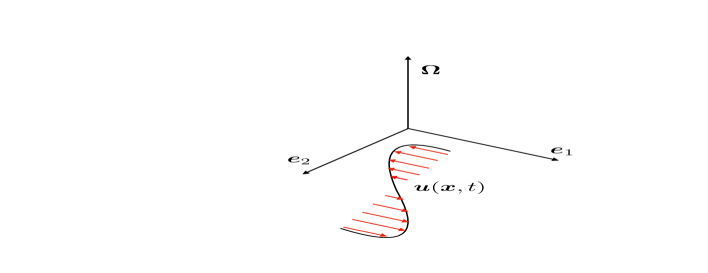
Figure 1: Sketch of a shear flow along the direction $\bm{e}_{1}$ in a reference frame with angular velocity $\bm{\Omega}$ along $\bm{e}_{3}$.

Under these hypotheses the tensor $\mathds{C}_{00}(t)$ in (39) has only one non vanishing component: $\mathds{C}_{00}^{11}(t)=C(t)$. Thus, upon introducing the vector

$$\bm{M}=\mathds{A}^{-1}\,\mathds{B}\,\bm{e}_{x}=\frac{1}{1+4/\text{Ro}^{2}}\left(\begin{aligned} &1+4\beta/\text{Ro}^{2}\\ &2(\beta-1)/\text{Ro}\\ &0\\ \end{aligned}\right)$$

Generalized Taylor’s formula takes the form

$${\mathds{D}}=\frac{D_{0}}{1+4/\text{Ro}^{2}}\mathds{1}+\bm{M}\otimes\bm{M}\int_{0}^{\infty}\mathrm{d}t\,C(t)\;$$ (41)

or, componentwise:

$$\mathds{D}=\frac{1}{1+4/\mathrm{\text{Ro}}^{2}}\times$$

$$\begin{bmatrix}D_{0}+\frac{(1+4\beta/\text{Ro}^{2})^{2}}{1+4/\text{Ro}^{2}}\int_{0}^{\infty}\mathrm{d}t\,C(t)&\frac{2(1+4\beta/\text{Ro}^{2})(\beta-1)/\text{Ro}}{1+4/\text{Ro}^{2}}\int_{0}^{\infty}\mathrm{d}t\,C(t)&0\\ \frac{2(1+4\beta/\text{Ro}^{2})(\beta-1)/\text{Ro}}{1+4/\text{Ro}^{2}}\int_{0}^{\infty}\mathrm{d}t\,C(t)&D_{0}+\frac{4(\beta-1)^{2}/\text{Ro}^{2}}{1+4/\text{Ro}^{2}}\int_{0}^{\infty}\mathrm{d}t\,C(t)&0\\ 0&0&D_{0}(1+4/\text{Ro}^{2})\\ \end{bmatrix}$$

It is instructive to analyze the behavior of the trace of the eddy diffusivity as a function of the Rossby number Ro:

$$\operatorname{Tr}{\mathds{D}}=D_{0}\left(1+\frac{2}{(1+4/\text{Ro}^{2})}\right)+\frac{(1+4\,\beta/\text{Ro}^{2})^{2}+4(\beta-1)^{2}/\text{Ro}^{2}}{(1+4/\text{Ro}^{2})^{2}}\int_{0}^{\infty}\mathrm{d}t\,C(t)$$

As a function of $\mathrm{Ro}$, $\operatorname{Tr}\mathds{D}$ turns out to be monotonic, at fixed $\beta$ and $D_{0}$. Indeed, its first derivative is :

$$-\frac{(\beta^{2}-1)\int_{0}^{\infty}\mathrm{d}t\,C(t)-2D_{0}}{(\text{Ro}^{2}+4)^{2}}8\ \text{Ro}$$

which has a constant sign, given that $\text{Ro}\geq 0$. In the limit of vanishing Rossby number (i.e. ideally an infinite value of $\Omega$), we get

$$\lim_{\mathrm{Ro}\downarrow 0}\operatorname{Tr}\mathds{D}=D_{0}+\beta^{2}\int_{0}^{\infty}\mathrm{d}t\,C(t)$$

The opposite limit of large Rossby (i.e. the absence of rotation), recovers the expression of the tracer particle model

$$\lim_{\mathrm{Ro}\uparrow\infty}\operatorname{Tr}\mathds{D}=3\,D_{0}+\int_{0}^{\infty}\mathrm{d}t\,C(t)$$

For $\beta<1$, $\operatorname{Tr}\mathds{D}$ always grows with respect to Ro. For light particles ($\beta>1$), instead, the $\operatorname{Tr}\mathds{D}$ may be monotonically decreasing or increasing depending upon whether the diffusion contribution from the flow $\int_{0}^{\infty}\mathrm{d}t\,C(t)$ is respectively higher or lower than the threshold value:

$$\frac{2D_{0}}{\beta^{2}-1}.$$

For incompressible carrier fields $\bm{u}$, $\int_{0}^{\infty}\mathrm{d}t\,C(t)$ is always positive. Hence, it is clear that only for $\beta>1$ a decreasing behavior is possible.

IV Maxey-Riley model

We now turn to the derivation of generalized Taylor’s formula for the now “canonical” Maxey–Riley model MaRi83 inclusive of the time derivatives along fluid trajectories and the Faxén friction Auton ; AuHuPr88 :

$$\begin{split}\frac{\mathrm{d}\bm{v}}{\mathrm{d}t}(t)&=\frac{\bm{u}(\bm{\xi}(t),t)-\bm{v}(t)+\frac{1}{6}r_{p}^{2}\nabla^{2}\bm{u}(\bm{\xi}(t),t)}{\tau}+\beta\frac{\mathrm{D}\bm{u}(\bm{\xi}(t),t)}{\mathrm{D}t}+\frac{\beta}{30}r_{p}^{2}\frac{\mathrm{d}}{\mathrm{d}t}\nabla^{2}\bm{u}(\bm{\xi}(t),t)\\ &+\sqrt{\frac{3\beta}{\pi\tau}}\int_{0}^{t}\frac{\mathrm{d}s}{\sqrt{t-s}}\,\frac{\mathrm{d}}{\mathrm{d}s}\Big{(}\bm{u}(\bm{\xi}(s),s)-\bm{v}(s)+\frac{1}{6}r_{p}^{2}\nabla^{2}\bm{u}(\bm{\xi}(s),s)\Big{)}+\frac{\sqrt{2D_{0}}}{\tau}\bm{\eta}(t)\end{split}$$ (42)

where $\frac{D}{Dt}=\partial_{t}+\bm{u}\cdot\bm{\nabla}$. With respect to the Basset-Boussinesq-Oseen equation, the latter term represents a higher order correction in the Stokes number, which still needs to be small MaRi83 . Higher order corrections in particles size are included, thanks to the Faxén drag force Gatignol . The reason is to take into account terms of order O($r^{2}_{p}/L^{2})$ whenever they could produce small but relevant deviations in comparison to the lower order approximation the Stokes drag provides. These higher-order corrections with respect to Stokes number and particle radius are often included in applications ToBo09 ; Guazzelli . For simplicity sake, we do not discuss here external forces. Upon removing the initial transient, taking Fourier–Laplace transform and recalling (18), we get into

$$\bm{\hat{v}}(z)=\frac{1}{a(z)}\left[\beta\widehat{\frac{\mathrm{D}\bm{u}}{\mathrm{D}t}}(z)+\left(a(z)-z-\frac{1}{\tau}\right)\left(\hat{\bm{u}}(z)+\frac{1}{6}r_{p}^{2}\widehat{\nabla^{2}\,\bm{u}}(z)\right)\right]$$ (43)

$$+ \frac{1}{\tau\,a(z)}\left[\hat{\bm{u}}(z)+\frac{1}{6}r_{p}^{2}\widehat{\nabla^{2}\,\bm{u}}(z)+\sqrt{2D_{0}}\,\bm{\hat{\eta}}(z)+z\,\frac{\beta}{30}\,r_{p}^{2}\,\widehat{\nabla^{2}\bm{u}}(z)\right]$$

Again the model can be couched into the form (4b) with all tensors $\mathds{K}_{i}$’s having the form of the identity matrix times scalar functions $K_{i}$ $i=0,\dots,3$. By comparing to Eqs. (19), we see that

$$\hat{K}_{0}(z)=1-\frac{z}{a(z)}$$ (44)

$$\hat{K}_{1}(z)=\frac{1}{\,a(z)} \hskip 5.69046pt\& \hat{\bm{f}}_{1}(z)=\beta\,\widehat{\frac{\mathrm{D}\bm{u}}{\mathrm{D}t}}(z)+\frac{\sqrt{2\,D_{0}}}{\tau}\,\bm{\hat{\eta}}(z)$$

$$\hat{K}_{2}(z)=\tau\,\hat{K}_{0}(z) \hskip 5.69046pt\& \bm{\hat{f}}_{2}(z)=\frac{1}{6\tau}r_{p}^{2}\widehat{\nabla^{2}\bm{u}}(z)$$

$$\hat{K}_{3}(z)=\frac{\tau\,z}{a(z)} \hskip 5.69046pt\& \bm{\hat{f}}_{3}(z)=\frac{\beta}{30\tau}\,r_{p}^{2}\widehat{\nabla^{2}\bm{u}}(z)$$

The scalar kernels satisfy

$$\hat{K}_{0}(0) = \int_{0}^{\infty}\mathrm{d}t\,K_{0}(t)=1$$

$$\hat{K}_{i}(0) = \int_{0}^{\infty}\mathrm{d}t\,K_{i}(t)=\tau\,\hskip 28.45274pti=1,2$$

whilst $\hat{K}_{3}(0)=0$. This latter fact implies that $\bm{f}_{3}$ does not give any contribution to generalized Taylor’s formula. Upon applying the general result (14), we get into

$${\mathds{D}}=D_{0}\mathds{1} + \operatorname{Sym}\int_{t_{0}}^{\infty}\mathrm{d}t\,\left\langle\left[\delta\bm{u}(\bm{\xi}(t),t)+\beta\tau\,\delta\frac{\mathrm{D}\bm{u}}{\mathrm{D}t}(\bm{\xi}(t),t)+\frac{1}{6}r_{p}^{2}\,\delta\nabla^{2}\bm{u}(\bm{\xi}(t),t)\right]\right.$$ (45)

$$\otimes \left.\left[\delta\bm{u}(\bm{\xi}(t_{0}),t_{0})+\beta\tau\,\delta\frac{\mathrm{D}\bm{u}}{\mathrm{D}t}(\bm{\xi}(t_{0}),t_{0})+\frac{1}{6}r_{p}^{2}\,\,\delta\nabla^{2}\bm{u}(\bm{\xi}(t_{0}),t_{0})\right]\right\rangle$$

where we considered the instant $t_{0}$ as the time at which the correlation functions can be considered stationary, and:

$$\delta\bm{u}(\bm{\xi}(t),t) = \bm{u}(\bm{\xi}(t),t)-\Big{\langle}\bm{u}(\bm{\xi}(t),t)\Big{\rangle}$$

$$\delta\frac{\mathrm{D}\bm{u}}{\mathrm{D}t}(\bm{\xi}(t),t) = \frac{\mathrm{D}\bm{u}}{\mathrm{D}t}(\bm{\xi}(t),t)-\Big{\langle}\frac{\mathrm{D}\bm{u}}{\mathrm{D}t}(\bm{\xi}(t),t)\Big{\rangle}$$ (46)

$$\delta\nabla^{2}\bm{u}(\bm{\xi}(t),t) = \nabla^{2}\bm{u}(\bm{\xi}(t),t)-\Big{\langle}\nabla^{2}\bm{u}(\bm{\xi}(t),t)\Big{\rangle}$$

By comparing Eqs. (45) and (27), we clearly see the Maxey–Riley and Basset–Boussinesq–Oseen models tend to coincide when $r_{p}/L$ and $\beta\tau/\tau_{F}$ are $\ll 1$, $\tau_{F}$ and $L$ being characteristic time and length scale of the flow, respectively.

Eq. (45) generalizes results previously given in literature (see e.g.BoMaMG17 ), where explicit expressions for the eddy diffusivity had been derived in the case of heavy particles. Indeed, that corresponds to $\beta=0$, and in such a limit only the Stokes drag in Eq. (42) survives.

V Models including lift forces

Further higher-order corrections due to particle size and higher Stokes numbers include lift forces. Some models were obtained in literature even in the case of small particle Reynolds numbers Re_p. The earliest model was provided by Saffman in 1965 Saffman ; SaffmanII for small solid particles in shear flows. This model is often used in its generalization to 3-dimensional flows Lift . A lot of different, empirical models have been proposed since then, taking into account different sizes and shapes of particles, wall effects, momentum transfer between the carrier fluid and the inner fluid inside the particle – which is meaningful if that particle is a bubble – or finite Reynolds numbers Legendre ; LiftWall ; Tomi ; MeiLift . Typically, these models have the following shape for the lift force on a spherical particle:

$$\bm{F}_{L}={C_{L}}\,\rho_{f}\,\frac{4}{3}\pi r_{p}^{3}[\bm{v}(t)-\bm{u}(\bm{\xi}(t),t)]\times\bm{\omega}(\bm{\xi}(t),t)$$ (47)

where $\bm{\omega}=\nabla\times\bm{u}$ is the vorticity and $C_{L}$ is the lift coefficient, which in general can be determined solely by fitting experimental data and it depends on several parameters of the carrier flow itself.

It is not in the scope of this article to provide a general view over lift force models, which is a vast phenomenology as said above. We rather want to provide an example about how to obtain an expression of the eddy diffusivity via the generalized Taylor’s formula. That would be useful to see how the autocorrelation and the mutual correlations of the several forces would act on the asymptotic diffusion. To do so, we stick to the Saffman model, for which Lift :

$$C_{L}=\frac{6.46}{\frac{4}{3}\,\pi r_{p}}\sqrt{\frac{\nu}{||\bm{\omega}(\bm{\xi}(t),t)||}}$$ (48)

The equation of motion turns out to be:

$$\begin{split}\frac{\mathrm{d}\bm{v}}{\mathrm{d}t}(t)&=\frac{\bm{u}(\bm{\xi}(t),t)-\bm{v}(t)+\frac{1}{6}r_{p}^{2}\nabla^{2}\bm{u}(\bm{\xi}(t),t)}{\tau}+\beta\frac{\mathrm{D}\bm{u}(\bm{\xi}(t),t)}{\mathrm{D}t}+\frac{\beta}{30}r_{p}^{2}\frac{\mathrm{d}}{\mathrm{d}t}\nabla^{2}\bm{u}(\bm{\xi}(t),t)\\ &+\sqrt{\frac{3\beta}{\pi\tau}}\int_{0}^{t}\frac{\mathrm{d}s}{\sqrt{t-s}}\,\frac{\mathrm{d}}{\mathrm{d}s}\Big{(}\bm{u}(\bm{\xi}(s),s)-\bm{v}(s)+\frac{1}{6}r_{p}^{2}\nabla^{2}\bm{u}(\bm{\xi}(s),s)\Big{)}\\ &+\frac{6.46\,\beta}{2\,\pi r_{p}}\sqrt{\frac{\nu}{||\bm{\omega}(\bm{\xi}(t),t)||}}[\bm{v}(t)-\bm{u}(\bm{\xi}(t),t)]\times\bm{\omega}(\bm{\xi}(t),t)+\frac{\sqrt{2D_{0}}}{\tau}\bm{\eta}(t)\\ \end{split}$$ (49)

Seeing that here the advection time scales are provided by the very vorticity, i.e. $\tau_{F}=\max(1/||\bm{\omega}||)$, and regcalling that $\tau=3r^{2}_{p}/(\nu\beta)$, the ratio between Saffman force per unity of mass and Stokes drag is:

$$\frac{\frac{2}{3}\beta\frac{6.46}{4/3\,\pi r_{p}}\sqrt{\frac{\nu}{||\bm{\omega}||}}||[\bm{v}-\bm{u}]\times\bm{\omega}||}{||\bm{u}-\bm{v}||/\tau}\leq\frac{2}{3}\beta\frac{6.46}{4/3\pi}\sqrt{\frac{\nu}{||\bm{\omega}||r_{p}^{2}}}\tau||\bm{\omega}||\sim O(\sqrt{\text{St}})$$ (50)

As a result of this, Saffman’s lift force is always negligible at sufficiently low Stokes times, or whenever $\rho_{p}\ll\rho_{f}$, that is $\beta\ll 1.$ For the Saffman model to hold true, along with Re${}_{p}\sim 0$ one needs:

$$\max\frac{||\bm{\Omega}_{p}||r_{p}^{2}}{||\bm{v}-\bm{u}||}\ll 1\qquad\&\qquad\max\frac{\sqrt{||\bm{\omega}||/\nu}}{||\bm{v}-\bm{u}||/\nu}\gg 1$$

having indicated the particle angular velocity by $\bm{\Omega}_{p}$.

We observe that we have one more forcing term in addition to those of the Maxey-Riley model in Eq. (44):

$$\hat{K}_{4}(z)=\hat{K}_{1}(z) \hskip 5.69046pt\& \bm{\hat{f}}_{4}(z)={\hat{\bm{f}}_{L}(z)}$$ (51)

where $\hat{\bm{f}}_{L}$ is the time Laplace transform of the lift force:

$$\bm{f}_{L}(\bm{\xi}(t),t)=\frac{6.46\,\beta}{2\,\pi r_{p}}\sqrt{\frac{\nu}{||\bm{\omega}(\bm{\xi}(t),t)||}}[\bm{v}(t)-\bm{u}(\bm{\xi}(t),t)]\times\bm{\omega}(\bm{\xi}(t),t)$$ (52)

A straightforward application of the generalized Taylor’s formula (14) yields:

$${\mathds{D}}=D_{0}\mathds{1} + \operatorname{Sym}\int_{t_{0}}^{\infty}\mathrm{d}t\,\left\langle\left[\delta\bm{u}(\bm{\xi}(t),t)+\beta\tau\,\delta\frac{\mathrm{D}\bm{u}}{\mathrm{D}t}(\bm{\xi}(t),t)+\frac{1}{6}r_{p}^{2}\,\delta\nabla^{2}\bm{u}(\bm{\xi}(t),t)+\tau\delta\bm{f}_{L}(\bm{\xi}(t),t)\right]\right.$$

$$\otimes \left.\left[\delta\bm{u}(\bm{\xi}(t_{0}),t_{0})+\beta\tau\,\delta\frac{\mathrm{D}\bm{u}}{\mathrm{D}t}(\bm{\xi}(t_{0}),t_{0})+\frac{1}{6}r_{p}^{2}\,\,\delta\nabla^{2}\bm{u}(\bm{\xi}(t_{0}),t_{0})+\tau\delta\bm{f}_{L}(\bm{\xi}(t_{0}),t_{0})\right]\right\rangle$$

Eq. (V) allows evaluating how the autocorrelation of the lift force and its cross-correlations with the other terms contribute to the eddy diffusivity. This can be carried out by the analysis of trajectories from available RADAR data or numerical simulations.

It should be noted that Eqs. (49) and (V) do not contain lift terms depending on the angular velocity $\bm{\Omega}_{p}$ of the particle, the so-called Magnus effect. Indeed, among higher order corrections (see. Eqs. (2.17)-(4.15) in Saffman and Eq. (4) in Lift ), a lift force acting on the particle of the form Magnus :

$$\rho_{f}r_{p}^{3}\pi\bm{\Omega}_{p}\times[\bm{v}(t)-\bm{u}(\bm{\xi}(t),t)]$$ (54)

should be added to Eq. (47). However, the ratio between this term per unity of mass and the Stokes drag is:

$$\frac{\frac{2}{3}\beta\pi r^{3}_{p}||\bm{\Omega}_{p}\times[\bm{v}(t)-\bm{u}(\bm{\xi}(t),t)]||}{\frac{4}{3}\pi r_{p}^{3}||\bm{v}(t)-\bm{u}(\bm{\xi}(t),t)||/\tau}\leq\beta||\bm{\Omega}_{p}||\tau\leq\beta\frac{||\bm{\Omega}_{p}||}{||\bm{\omega}||}\text{St}$$ (55)

This ratio turns out to be of order $O$(St), while the one between Saffman lift and Stokes drag was $\sim O(\sqrt{\text{S}t})$. This justifies why the Magnus term (55) is often neglected for small solid particles, unless the angular velocity is high. However, for a freely rotating sphere, $\bm{\Omega}_{p}=1/2\,\bm{\omega}$ Saffman . We did not take that term into account here for the sake of simplicity, it being often ignored. In any case, its inclusion in Eq. (V) is trivially inside the addend $\bm{f}_{L}$.

VI Conclusions

We analyzed general conditions under which a generalized Taylor’s eddy diffusivity formula applies to inertial particle models.

It is worth emphasizing that Taylor’s formula for the Basset–Boussinesq–Oseen model of inertial particle dynamics with the inclusion of the Brownian force, is formally the same as the Taylor’s formula for tracer particles. The equivalence is, however, only formal. Since the time integral of the fluid velocity autocorrelation function is carried out along particle trajectories, the well-known mismatch between fluid and particle trajectories leads in general to different eddy diffusivities.

In the case of the Maxey-Riley model, new terms appear in the expression for the eddy diffusivity with respect to the tracer case and thus with respect to the Basset–Boussinesq–Oseen model. We also discussed under which coditions the two models admit the same formal expression for the eddy diffusivity. Similar conclusions were drawn taking into account lift forces.

Our analysis encompasses, as special cases of interest in applications, the two relevant examples of particle dynamics forced by the Coriolis contribution (for application to dispersions in geophysical flows) and the Lorentz force (for application to dispersions of charged particles in electrically neutral flows). In this latter case, we proved that in the limit of small inertia (i.e. $\mathrm{St}\,\downarrow\,0$) and magnetic field $\bm{B}^{*}$ such that $\|\bm{B}^{*}\|$ is independent of $\mathrm{St}$, the inertial particle dynamics reduces to a tracer dynamics with a carrier flow which now becomes compressible. Clustering phenomena induced by the magnetic field are thus expected to emerge. For a vanishing carrier flow, the combined roles of Brownian motion and magnetic field has been proved to give rise to a smaller eddy diffusivity than the molecular diffusivity $D_{0}$. Transport depletion is thus expected in applications involving the magnetic field. Similar conclusions can be obtained for the Coriolis contribution. The mathematical structure of this term is indeed very similar to the Lorentz force. Taylor’s formula for tracer dispersion has ubiquitous applications in the study of turbulent transport. We thus expect that our analysis will be useful for further investigations of large-scale transport properties of inertial particles under the action of different forcing mechanisms.

Appendix A

Proposition 1

Under the hypotheses I-II-III, generalized Taylors’s identity (14) holds true for any dynamical model of the form (4)

To prove the claim, we need first to couch (10) into the form (11) which is more adapted to discuss the large time limit. This is done by first applying to (10) the double integral inversion formula over a triangular domain

$$\operatorname{Sym}\int_{0}^{t}\mathrm{d}s\,\langle\,\delta\bm{v}(t)\otimes\delta\bm{v}(s)\rangle=$$ (1)

$$\sum_{ij=0}^{N}\operatorname{Sym}\int_{0}^{t}\mathrm{d}s_{3}\,\int_{0}^{t}\mathrm{d}s_{2}\int_{s_{2}}^{t}\mathrm{d}s_{1}\,\mathds{K}_{i}(t-s_{3})\,\tilde{\mathds{C}}_{ij}(s_{3},s_{2})\,\mathds{K}_{j}^{T}(s_{1}-s_{2})$$

Performing the sequence the change of variables $s_{1}=u_{1}+s_{2}$, $s_{2}=t-u_{2}$ and $s_{3}=t-u_{3}$ yields (11) which, for reading convenience, we re-write here as

$$\operatorname{Sym}\int_{0}^{t}\mathrm{d}s\,\langle\,\delta\bm{v}(t)\otimes\delta\bm{v}(s)\rangle=$$ (2)

$$\sum_{ij=0}^{N}\operatorname{Sym}\int_{0}^{t}\mathrm{d}u_{3}\,\int_{0}^{t}\mathrm{d}u_{2}\int_{0}^{u_{2}}\mathrm{d}u_{1}\,\mathds{K}_{i}(u_{3})\,\tilde{\mathds{C}}_{ij}(t-u_{3},t-u_{2})\,\mathds{K}_{j}^{T}(u_{1})$$

We now invoke hypotheses I-II. They ensure that (2) (or equivalently (11)) is absolutely integrable in the large time limit. Before proving this claim, it is convenient to proceed to analyze its implications. Namely, if we take the limit under the integral and invoke hypothesis III, upon applying once again the double integral inversion formula over a triangular domain, we obtain

$$\mathds{D}=\lim_{t\uparrow\infty}\operatorname{Sym}\int_{0}^{t}\mathrm{d}s\,\langle\,\delta\bm{v}(t)\otimes\delta\bm{v}(s)\rangle$$ (3)

$$=\sum_{ij=0}^{N}\operatorname{Sym}\int_{0}^{\infty}\mathrm{d}u_{3}\,\int_{0}^{\infty}\mathrm{d}u_{1}\,\mathds{K}_{i}(u_{3})\,\mathds{F}_{ij}(u_{3},u_{1})\,\mathds{K}_{j}^{T}(u_{1})$$

where by (13)

$$\mathds{F}_{ij}(u_{3},u_{1})=\int_{u_{1}}^{\infty}\mathrm{d}u_{2}\left\{\begin{array}[]{ll}\mathds{C}_{ij}(u_{2}-u_{3})&\hskip 5.69046pt\forall\,u_{2}\geq u_{3}\\[8.5359pt] \mathds{C}_{ji}^{T}(u_{3}-u_{2})&\hskip 5.69046pt\forall\,u_{2}<u_{3}\end{array}\right.$$ (6)

The kernel (6) is in fact a function of $u_{1}-u_{3}$ alone and admits important simplifications. Namely, we notice that for $u_{1}\,\geq\,u_{3}$

$$\mathds{F}_{ij}(u_{3},u_{1})=\int_{0}^{\infty}\mathrm{d}u\,\mathds{C}_{ij}(u)-\int_{0}^{u_{1}-u_{3}}\mathrm{d}u\,\mathds{C}_{ij}(u)$$

whilst for $u_{3}\,>\,u_{1}$ we find

$$\mathds{F}_{ij}(u_{3},u_{1})=\int_{0}^{\infty}\mathrm{d}u\,\mathds{C}_{ij}(u)+\int_{0}^{u_{3}-u_{1}}\mathrm{d}u\,\mathds{C}_{ji}^{T}(u)$$

Upon gleaning these observations, we conclude after a further application of (13) that

$$\mathds{F}_{ij}(u_{3},u_{1})=\int_{0}^{\infty}\mathrm{d}u\,\mathds{C}_{ij}(u)-\int_{0}^{u_{1}-u_{3}}\mathrm{d}u\,\mathds{C}_{ij}(u)\equiv\mathds{\hat{C}}_{ij}(0)-\tilde{\mathds{F}}_{ij}(u_{1}-u_{3})$$ (7)

where furthermore

$$\tilde{\mathds{F}}_{ij}(-t)=\int_{0}^{-t}\mathrm{d}u\,\mathds{C}_{ij}(u)=-\int_{0}^{t}\mathrm{d}u\,\mathds{C}_{ij}(-u)=-\int_{0}^{t}\mathrm{d}u\,\mathds{C}_{ji}^{T}(u)=-\tilde{\mathds{F}}_{ji}^{T}(t)$$ (8)

We have now forged all the tools needed to prove the proposition. If we take the $\operatorname{Sym}$ operation under the integral sign and rename dummy integration/summation variables, we get into

$$\mathds{D}=\sum_{ij=0}^{N}\int_{0}^{\infty}\mathrm{d}u_{3}\int_{0}^{\infty}\mathrm{d}u_{1}\,\mathds{K}_{i}(u_{3})\,\frac{\mathds{F}_{ij}(u_{3},u_{1})+\mathds{F}_{ji}^{T}(u_{1},u_{3})}{2}\,\mathds{K}_{j}^{T}(u_{1})$$ (9)

In view of (7), (8) the chain of identities

$$\frac{\mathds{F}_{ij}(u_{3},u_{1})+\mathds{F}_{ji}^{T}(u_{1},u_{3})}{2}=$$ (10)

$$\frac{\mathds{\hat{C}}_{ij}(0)+\mathds{\hat{C}}_{ji}^{\mathsf{T}}(0)}{2}-\frac{\mathds{\tilde{F}}_{ij}(u_{1}-u_{3})+\mathds{\tilde{F}}_{ji}^{T}(u_{3}-u_{1})}{2}=$$

$$\frac{\mathds{\hat{C}}_{ij}(0)+\mathds{\hat{C}}_{ji}^{\mathsf{T}}(0)}{2}-\frac{\mathds{\tilde{F}}_{ij}(u_{1}-u_{3})-\mathds{\tilde{F}}_{ij}(u_{1}-u_{3})}{2}=\frac{\mathds{\hat{C}}_{ij}(0)+\mathds{\hat{C}}_{ji}^{\mathsf{T}}(0)}{2}$$

holds true. Hence, the kernel in (10) is independent of the integration variables $u_{1}$, $u_{3}$ and the double integral factorizes in the product of two integrals. As a consequence, (10) reduces to generalized Taylor’s formula (14), as claimed.

Finally, we can return to the proof that hypotheses I-II are sufficient to guarantee that it is safe to apply the dominated convergence theorem to (2). Namely, the chain of inequalities

$$\left|\int_{0}^{t}\mathrm{d}s\Big{\langle}\delta{v}^{m}(t)\;\delta{v}^{n}(s)\Big{\rangle}\,\right|$$ (11)

$$\leq\sum_{ij=0}^{N}\int_{0}^{t}\mathrm{d}s_{3}\int_{0}^{t}\mathrm{d}s_{1}\int_{0}^{s_{1}}\mathrm{d}s_{2}\,|\mathds{K}_{i}^{ml}(s_{3})|\,|\mathds{K}_{j}^{nk}(s_{1})|\,|\tilde{\mathds{C}}^{l\,k}_{i\,j}(s_{3},s_{2})|$$

$$\leq\int_{0}^{t}\mathrm{d}s_{3}\int_{0}^{t}\mathrm{d}s_{1}V^{m}(s_{3})\,V^{n}(s_{1})\,\int_{0}^{s_{1}}\mathrm{d}s_{2}\,F(s_{3}-s_{2})$$

holds for

$$V^{n}(t)=\sum_{i=0}^{N}\sum_{l=1}^{d}|\mathds{K}_{i}^{nl}(t)|$$

The innermost integral in (11) satisfies

$$0\leq\int_{0}^{s_{1}}\mathrm{d}s_{2}\,F(s_{3}-s_{2})\,<\,\int_{-\infty}^{\infty}\mathrm{d}s\,F(s)\equiv 2\,f_{\star}$$

since $F$ is positive, even and integrable by hypothesis. We conclude that

$$\lim_{t\uparrow\infty}\left|\int_{0}^{t}\mathrm{d}s\Big{\langle}\delta{v}^{m}(t)\;\delta{v}^{n}(s)\Big{\rangle}\,\right|\,<\,2\,[(N+1)\,K_{\star}\,d]^{2}\,f_{\star}\,<\,\infty\,,$$

with $K_{*}$ being defined in Eq. (5).

TABLE OF GENERALIZED TAYLOR FORMULAE
Model	Eddy diffusivity
Basset-Boussinesq-Oseen equation	$\lim_{t\uparrow\infty}\operatorname{Sym}\int_{0}^{t}\mathrm{d}s\,\langle\,\delta\bm{u}(\bm{\xi}(s),s)\otimes\delta\bm{u}(\bm{\xi}(t),t)\rangle\;\;\;$
plus white noise and constant gravity
Basset-Boussinesq-Oseen equation	$\frac{D_{0}}{\tau^{2}}\mathds{\hat{A}}^{-1}(0)\,(\mathds{\hat{A}}^{-1})^{T}(0)+\frac{1}{\tau^{2}}\mathds{\hat{A}}^{-1}(0)\operatorname{Sym}\Big{(}\hat{\mathds{C}}_{00}(0)\Big{)}\,(\mathds{\hat{A}}^{-1})^{T}(0)$
plus white noise and Lorentz force	where
	$(\mathds{\hat{A}}^{-1})^{\mu\nu}(z)=\frac{1}{a^{2}(z)+\gamma^{2}\,\|\bm{B}\|^{2}}\left[a(z)\,\delta^{\mu\nu}-\gamma\,B^{i}\,\epsilon^{\mu\sigma\nu}+\frac{\gamma^{2}}{a(z)}B^{k}\,B^{j}\right]$
	$a(z)=z+\frac{1}{\tau}+\sqrt{\frac{3\beta z}{\pi\tau}}$
	$\gamma=\frac{q}{\frac{4}{3}\pi r^{3}_{p}\rho_{p}}$
Basset-Boussinesq-Oseen equation
plus white noise and Lorentz force	$\text{diag}\left(\frac{D_{0}}{1+\gamma^{2}\,B^{2}\,\tau^{2}},\frac{D_{0}}{1+\gamma^{2}\,B^{2}\,\tau^{2}},D_{0}\right)$
(flow at rest, constant magnetic field $\bm{B}=(0,0,B)$ )
Basset-Boussinesq-Oseen equation	$D_{0}\;\mathds{A}^{-1}({\mathds{A}}^{-1})^{T}+\mathds{A}^{-1}\operatorname{Sym}\Big{(}\hat{\mathds{C}}_{00}(0)\Big{)}({\mathds{A}}^{-1})^{T}$
plus white noise and Lorentz force	where
(limit of vanishing Stokes number and $\bm{B}*=\gamma\tau\bm{B}$ )	$\mathds{A}^{\mu\nu}=\delta^{\mu\nu}+B^{*\,i}\,\epsilon^{\mu\sigma\nu}$

Model	Eddy diffusivity
Basset-Boussinesq-Oseen equation	$\frac{D_{0}}{\tau^{2}}\mathds{\hat{A}}^{-1}(0)\,({\mathds{\hat{A}}}^{-1})^{T}(0)+\mathds{\hat{A}}^{-1}(0)\,\mathds{\hat{B}}(0)\,\operatorname{Sym}\Big{(}\hat{\mathds{C}}_{00}(0)\Big{)}\,\mathds{\hat{B}}^{T}(0)\,({\mathds{\hat{A}}}^{-1})^{T}(0)$
plus constant gravity, white noise and Coriolis force,	where
Basset force neglected	$\mathds{\hat{A}}^{\mu\nu}(z)=\left(z+\frac{1}{\tau}\right)\,\delta^{\mu\nu}+2\,\Omega^{\sigma}\,\epsilon^{\mu\sigma\nu}$
	$\mathds{\hat{B}}^{\mu\nu}(z)=\left(\beta\,z+\frac{1}{\tau}\right)\,\delta^{\mu\nu}+2\,\beta\,\Omega^{\sigma}\,\epsilon^{\mu\sigma\nu}$
Basset-Boussinesq-Oseen equation
plus white noise, constant gravity and Coriolis force	$\text{diag}\left(\frac{D_{0}}{1+4\,\Omega^{2}\,\tau^{2}},\frac{D_{0}}{1+4\,\Omega^{2}\,\tau^{2}},D_{0}\right)$
(flow at rest,constant angular velocity $\bm{\Omega}=(0,0,\Omega)$ )
Basset-Boussinesq-Oseen equation	$\frac{D_{0}}{1+4/\text{Ro}^{2}}\mathds{1}+\bm{M}\otimes\bm{M}\int_{0}^{\infty}\mathrm{d}t\,C(t)$
plus white noise, constant gravity and Coriolis force,	where
Basset force neglected.	$\bm{M}=\frac{1}{1+4/\text{Ro}^{2}}\left(\begin{aligned} &1+4\beta/\text{Ro}^{2}\\ &2(\beta-1)/\text{Ro}\\ &0\\ \end{aligned}\right)$
(shear flow $\bm{u}(\bm{x},t)=u(x_{2},x_{3},t)\bm{e}_{1}\;,$	$C(t)=\lim_{t^{\prime}\to\infty}\langle\delta u(\bm{\xi}(t^{\prime}),t^{\prime})\delta u(\bm{\xi}(t+t^{\prime}),t+t^{\prime})\rangle$
constant angular velocity $\bm{\Omega}=(0,0,\Omega)$ ,
fixed Rossby number $\mathrm{Ro}=1/(\tau\,\Omega)$ )

Model	Eddy diffusivity
Maxey-Riley equation	$D_{0}\mathds{1}+\operatorname{Sym}\int_{t_{0}}^{\infty}\mathrm{d}t\,$
(including white noise, Faxén, and Auton terms)	$\left\langle\left[\delta\bm{u}(\bm{\xi}(t),t)+\beta\tau\,\delta\frac{\mathrm{D}\bm{u}}{\mathrm{D}t}(\bm{\xi}(t),t)+\frac{1}{6}r_{p}^{2}\,\delta\nabla^{2}\bm{u}(\bm{\xi}(t),t)\right]\right.$
	$\otimes\left.\left[\delta\bm{u}(\bm{\xi}(t_{0}),t_{0})+\beta\tau\,\delta\frac{\mathrm{D}\bm{u}}{\mathrm{D}t}(\bm{\xi}(t_{0}),t_{0})+\frac{1}{6}r_{p}^{2}\,\,\delta\nabla^{2}\bm{u}(\bm{\xi}(t_{0}),t_{0})\right]\right\rangle$
Maxey-Riley equation + lift force	${\mathds{D}}=D_{0}\mathds{1}+\operatorname{Sym}\int_{t_{0}}^{\infty}\mathrm{d}t\,$
	$\left\langle\left[\delta\bm{u}(\bm{\xi}(t),t)+\beta\tau\,\delta\frac{\mathrm{D}\bm{u}}{\mathrm{D}t}(\bm{\xi}(t),t)\right.\right.$
	$\left.\left.+\frac{1}{6}r_{p}^{2}\,\delta\nabla^{2}\bm{u}(\bm{\xi}(t),t)+\tau\delta\bm{f}_{L}(\bm{\xi}(t),t)\right]\right.$
	$\otimes\left.\left[\delta\bm{u}(\bm{\xi}(t_{0}),t_{0})+\beta\tau\,\delta\frac{\mathrm{D}\bm{u}}{\mathrm{D}t}(\bm{\xi}(t_{0}),t_{0})\right.\right.$
	$\left.\left.+\frac{1}{6}r_{p}^{2}\,\,\delta\nabla^{2}\bm{u}(\bm{\xi}(t_{0}),t_{0})+\tau\delta\bm{f}_{L}(\bm{\xi}(t_{0}),t_{0})\right]\right\rangle$

References

• (1) G. I. Taylor, Diffusion by continuous movements, Proceedings of the London Mathematical Society 20, 196–212 (1922).
• (2) L. Biferale, A. Crisanti, M. Vergassola, and A Vulpiani, Eddy diffusivities in scalar transport, Physics of Fluids 7, 2725-2734 (1995).
• (3) S. Boi, A. Mazzino and G. Lacorata, Explicit expressions for eddy-diffusivity fields and effective large-scale advection in turbulent transport, Journal of Fluid Mechanics 795, 524-548 (2016).
• (4) M. Cencini, A. Mazzino, S. Musacchio and A. Vulpiani, Large-scale effects on meso-scale modeling for scalar transport, Physica D 220, 146-156 (2006).
• (5) U. Frisch, Lecture on turbulence and lattice gas hydrodynamics. In Lecture Notes, NCAR-GTP Summer School June 1987 (ed. J. R. Herring & J. C. McWilliams), pp. 219–371. World Scientific.
• (6) A. Mazzino, Effective correlation times in turbulent scalar transport, Physical Review E 56(5), 5500-5510 (1997).
• (7) A. Mazzino, S. Musacchio and A. Vulpiani, Multiple-scale analysis and renormalization for preasymptotic scalar transport, Physical Review E 71, 011113 (2005).
• (8) R.H. Kraichnan, R. H. Eddy viscosity and diffusivity: exact formulas and approximations Complex Systems, 1, 805-820, (1987).
• (9) J. Majda and P. R. Kramer, Simplified models for turbulent diffusion: Theory, numerical modelling, and physical phenomena, Physics Reports 314, 237-574 (1999).
• (10) P.K. Kundu, I.M. Cohen and D.R. Dowling, Fluid mechanics 6th edition, Academic Press (2012).
• (11) F. Toschi and E. Bodenschatz, Lagrangian Properties of Particles in Turbulence, Annual Review of Fluid Mechanics 41, 375-404 (2009).
• (12) IPCC: Fifth assessment report – the physical science basis, available at: http://www.ipcc.ch (last access: 14 December 2015), (2013).
• (13) G. Falkovich, A. Fouxon and M.G. Stepanov, Acceleration of rain initiation by cloud turbulence, Nature 419, 151-154 (2002).
• (14) A. Celani, G. Falkovich, A. Mazzino and A. Seminara, Droplet condensation in turbulent flows. Europhysics Letters 70, 775-781 (2005).
• (15) A. Celani, A. Mazzino and M. Tizzi, The equivalent size of cloud condensation nuclei. New Journal of Physics 10, 075021 (2008)
• (16) I. Fouxon and A. Leshansky, Phytoplankton’s motion in turbulent ocean, Physical Review E 92, 013017 (2015).
• (17) A. Bracco, P.H. Chavanis, A. Provenzale and E.A. Spiegel, Particle aggregation in a turbulent Keplerian flow, Physics of Fluids 11, 2280 (1999).
• (18) M. Wilkinson, B. Mehlig and V. Uski, Stokes Trapping and Planet Formation, The Astrophysical Journal Supplement Series 176, 484-496 (2008).
• (19) B.T. Chao, Turbulent transport behaviour of small particles in dilute suspension, Österreichisches Ingenieur-Archiv 18, 7-21 (1964).
• (20) C. M. Tchen, Mean value and correlation problems connected with the motion of small particles suspended in a turbulent fluid, Ph.D. Thesis, University of Delft, Martinus Nijhoff, The Hague (1947).
• (21) J.O. Hinze, Turbulence, Mcgraw-Hill College, 790 (1975).
• (22) R. Mei, R.J. Adrian, and T.J. Hanratty, Particle dispersion in isotropic turbulence under Stokes drag and Basset force with gravitational settling Journal of Fluid Mechanics 225, 481 (1991).
• (23) L.M. Pismen and A. Nir, On the motion of suspended particles in stationary homogeneous turbulence Journal of Fluid Mechanics, 84, 193 (1978).
• (24) M.W. Reeks, On the dispersion of small particles suspended in an isotropic turbulent fluid, Journal of Fluid Mechanics 83, 529-546 (1977).
• (25) M.W. Reeks, The relationship between Brownian motion and the random motion of small particles in a turbulent flow, Physics of Fluids 31, 1314–1316 (1988).
• (26) L.-P. Wang and D.E. Stock, Dispersion of Heavy Particles by Turbulent Motion, Journal of the Atmospheric Sciences 50, 1897-1913 (1993).
• (27) L. Corgnati, C. Mantovani, A. Griffa, P. Penna, P. Celentano, L. Bellomo, D.F. Carlson, R. D’Adamo, Implementation and validation of the ISMAR High Frequency Coastal Radar Network in the Gulf of Manfredonia (Mediterranean Sea). IEEE Journal of Oceanic Engineering (2018).
• (28) A. Mazzino and M. Vergassola, Interference between turbulent and molecular diffusion. Europhysics Letters 37, 535-540 (1997).
• (29) M. R. Maxey and J. J. Riley, Equation of motion for a small rigid sphere in a nonuniform flow, Physics of Fluids 26(4), 883–889 (1983).
• (30) T. R. Auton, Dynamics of bubbles, drops, and particles in motion in liquids, Ph.D. thesis, University of Cambridge, Cambridge, UK (1984).
• (31) T.R. Auton, J.C.R. Hunt, and M. Prud’Homme, The force exerted on a body in inviscid unsteady non-uniform rotational flow. Journal of Fluid Mechanics 197, 241–257 (1988).
• (32) E.E. Michaelides, Hydrodynamic Force and Heat/Mass Transfer From Particles, Bubbles, and Drops—The Freeman Scholar Lecture. Journal of Fluids Engineering 25(2), 209-238 (2003).
• (33) F. Candelier, J. Einarsson, and B. Mehlig, Angular Dynamics of a Small Particle in Turbulence. Physical Review Letters 117, 204501 (2016)
• (34) P. Castiglione, A. Mazzino, P. Muratore-Ginanneschi and A. Vulpiani, On strong anomalous diffusion, Physica D: Nonlinear Phenomena 134, 75-93 (1999).
• (35) G. Biroli, A crash course on ageing, Journal of Statistical Mechanics: Theory and Experiment, P05014 (2005).
• (36) G. Falkovich, K. Gawȩdzki and M. Vergassola, Particles and fields in fluid turbulence, Reviews of Modern Physics 73, 913 (2001).
• (37) R. Kubo, M. Toda, and N. Hashitsume, Statistical Physics II - Nonequilibrium Statistical Mechanics, Springer-Verlag Berlin Heidelberg (1991).
• (38) M. R. Maxey, The motion of small spherical particles in a cellular flow field, Physics of Fluids 30 (7), 1915-1928 (1987).
• (39) M. Farazmand and G. Haller, The Maxey–Riley equation: Existence, uniqueness and regularity of solutions, Nonlinear Analysis: Real World Applications 22, 98-106 (2015).
• (40) M. Martins Afonso, A. Mazzino and P. Muratore-Ginanneschi, Eddy diffusivities of inertial particles under gravity, Journal of Fluid Mechanics 73, 426-463 (2012).
• (41) L. Bergougnoux, G. Bouchet, D. Lopez, and E. Guazzelli, The motion of solid spherical particles falling in a cellular flow field at low Stokes number. Physics of Fluids 26, 093302 (2014)
• (42) R. Czopnik and P. Garbaczewski, Brownian motion in a magnetic field, Physical Review E 63, 187-198 (2001).
• (43) B. Kursunoglu, Brownian motion in a magnetic field, Annals of Physics 17, 259–268 (1962).
• (44) D. S. Lemons and D. L. Kaufman, Brownian motion of a charged particle in a magnetic field, IEEE Transactions on Plasma Science 27 (5), 128-1296 (1999).
• (45) P. S. Alekseev, Negative Magnetoresistance in Viscous Flow of Two-Dimensional Electrons, Physical Review Letters 117, 166601 (2016).
• (46) W.B. Russel, Brownian Motion of Small Particles Suspended in Liquids, Annual Review of Fluid Mechanics 13, 425–455 (1981).
• (47) L. E. Reichl, A Modern Course in Statistical Physics (4th edition), Wiley (2016).
• (48) O. A. Druzhinin , andL. A. Ostrovsky, The influence of Basset force on particle dynamics in two-dimensional flows. Physica D 76, 34-43 (1994).
• (49) S. Boi, M. Martins Afonso, and A. Mazzino, Anomalous diffusion of inertial particles in random parallel flows: theory and numerics face to face. Journal of statistical mechanics: theory and experiment, P10023 (2015).
• (50) P. Monroy, E. Hernandez-Garcia, V. Rossi and C. Lopez, Modeling the dynamical sinking of biogenic particles in oceanic flow, Nonlinear Processes in Geophysics 24, 293-305 (2017).
• (51) R. Gatignol, The Faxén formulas for a rigid particle in an unsteady non-uniform Stokes-flow. Journal de mécanique théorique et appliquée 2 (2), 143–160 (1983).
• (52) S. Boi, A. Mazzino and P. Muratore-Ginanneschi, Eddy diffusivities of inertial particles in random Gaussian flows, Physical Review Fluids 2 (1), 014602 (2017).
• (53) P. G. Saffman, The lift on a small sphere in a slow shear flow. Journal of Fluid Mechanics 22, 385 (1965).
• (54) P. G. Saffman, Corrigendum to: “The lift on a small sphere in a slow shear flow”. Journal of Fluid Mechanics 31, 624 (1968).
• (55) K. L.Henderson, D. R. Gwynllyw, and C. F.Barenghi, Particle tracking in Taylor–Couette flow. European Journal of Mechanics - B/Fluids 26 (6), 738-748 (2007).
• (56) D. Legendre, J. and Magnaudet, The lift force on a spherical bubble in a viscous linear shear flow. Journal of Fluid Mechanics 368, 81–126 (1998).
• (57) A. Tomiyama, Struggle with computational bubble dynamics. ICMF’98, 3rd International Conference of Multiphase Flow, Lyon, France, pp. 1-18, June 8-12 (1998)
• (58) D. Leighton and A. Acrivos, The lift on a small sphere touching a plane in the presence of a simple shear flow . Journal of Applied Mathematics and Physics 36, 174 (1985)
• (59) R. Mei, An approximate expression for the shear lift force on a spherical particle at finite Reynolds number. International Journal of Multiphase Flow, 18(1), 145–147 (1992).
• (60) N. Lukerchenko , Y. Kvurt , I. Keita , Z. Chara, and P. Vlasak, Drag Force, Drag Torque, and Magnus Force Coefficients of Rotating Spherical Particle Moving in Fluid. Particulate Science and Technology 30, 55-67 (2012).