Portable multi-node LQCD Monte Carlo simulations using OpenACC

Abstract

This paper describes a state-of-the-art parallel Lattice QCD Monte Carlo code for staggered fermions, purposely designed to be portable across different computer architectures, including GPUs and commodity CPUs. Portability is achieved using the OpenACC parallel programming model, used to develop a code that can be compiled for several processor architectures. The paper focuses on parallelization on multiple computing nodes using OpenACC to manage parallelism within the node, and OpenMPI to manage parallelism among the nodes. We first discuss the available strategies to be adopted to maximize performances, we then describe selected relevant details of the code, and finally measure the level of performance and scaling-performance that we are able to achieve. The work focuses mainly on GPUs, which offer a significantly high level of performances for this application, but also compares with results measured on other processors.

PACS Nos.: 07.05.Bx 12.38.Gc

1 Introduction

Monte Carlo simulations play a key role in the study of several aspects of Quantum Chromodynamics (QCD), the quantum field theory that describes the strong interaction in the standard model of particle physics. Lattice QCD is a computational scheme based on importance sampling Monte Carlo simulations used to study QCD in the non-perturbative regime, i.e. when the theory is strongly interacting and perturbation theory cannot be applied. This approach has been extremely effective in obtaining first principles calculations of the hadron masses[1, 2] and of the thermodynamical properties of the quark-gluon plasma[3], while technical difficulties are still encountered when a large baryon chemical potential is present[4]. Despite the continuous efforts in the development of more and more efficient algorithms[5], Lattice QCD simulations still require a tremendous amount of computing resources.

Lattice QCD simulations belong to the class of HPC grand challenge applications, with physics results strongly limited by available computational resources[6, 7]. For this reason in the mid ’80s the increasing request for computational resources triggered the development of massively parallel supercomputers [8, 9, 10, 11, 12, 13] specifically designed and optimized to match the computing requirements of Lattice QCD algorithms. This approach lost its effectiveness as general purpose supercomputers started to be available on the market; interestingly enough, the architectures of these commercial machines were still similar to the ones of their LQCD-optimized predecessors, with low frequency and low power CPUs in each node and toroidal interconnection between the nodes. Nowadays we are in the middle of a new change of paradigm in the field of High Performance Computing (HPC), in which the typical node-to-node communication harness is all-to-all, and “slim” computing nodes are being replaced by “fat” ones, based on multi- and many-core CPUs or Graphic Processing Units (GPUs).

While the most recent CPU and GPU architectures seem to follow a converging evolutionary path, with an always increasing level of vectorization, different programming languages are still used to develop applications for CPUs and GPUs. This poses significant portability issues, that need to be seriously addressed, as there is still no clear consensus on the computing architectures – CPUs or GPUs – that will be mostly adopted in the near future.

The OpenACC[14] standard is a solution designed to address portability issues across several computing architectures, using a programming model similar to OpenMP[15], but specifically designed to allow applications to run on accelerators. It abstracts code functionalities to a descriptive level, leaving architecture-specific implementations to the compiler. Using this approach, the same source code may run on all processors, GPUs and also CPUs, supported by the compiler, achieving an easy and good level of code portability. OpenACC is becoming increasingly popular among several scientific communities for coding many lattice-based applications to run mainly on GPU accelerators, including Lattice Boltzmann Methods[16, 17, 18], and more recently also Lattice QCD [19, 20].

The change from “slim” to “fat” nodes, however, does not affect only the portability of the code, but also its parallel structure. In fact: i) the traditional strategy to minimize the surface over volume ratio of the tiles is no more a priori the optimal approach to get the best parallel efficiency, ii) different levels of parallelization must be exploited, ii) and data organization plays an increasing relevant role for computing performances.

In our previous work[20] we have described an OpenACC implementation of a state-of-the-art Monte Carlo Lattice QCD application, derived from an earlier version coded using CUDA[21], and able to run only on single-accelerator systems, including GPUs (NVIDIA and AMD), and also CPUs. In this paper we extend our OpenACC code to run also on accelerators-based parallel computing machines, discussing in detail how we have structured the code, the strategies that have guided our design choices, and presenting several performance results on different computing architectures. We focus mainly on GPU-based clusters since for this kind of applications they offer a level of performances an order of magnitude higher than standard high-end commodity CPUs. We describe how we distribute the workload of the application among the GPUs, the strategies used to overlap communications and computation, and analyze computing efficiency and strong scalability on several nodes. As in the previous work, we use the PGI compiler able to target all versions of NVIDIA GPUs as well as commodity CPUs, offering code portability and the possibility to measure, compare and analyze also performance figures of clusters based on recent multi-core Intel Xeon CPUs.

The structure of this paper is as follows: in Sec. 2 we briefly recall the global structure of Lattice QCD simulation algorithm, mainly focusing on those aspects that are relevant for parallelization; in Sec. 3 we analyze several parallelization strategies to distribute the data-domain over several computing-nodes and the tools available to exchange data, and in Sec. 4 we describe the details of our implementation. Finally, in Sec. 5 we analyze the parallel efficiency and scaling figures of the code, and in Sec. 6 we draw our conclusions.

2 Algorithms for Lattice QCD

In this section we summarize the basic algorithmic ingredients of a typical Lattice QCD simulation that are needed to understand the parallel structure of our implementation. We will use the same notation of a previous paper describing a single device implementation[20], to which we refer for more details and reference to the original literature[22, 23].

In a Lattice QCD simulation the space-time continuum is approximated by a lattice of spacing $a$ and extents $aN_{t},aN_{x},aN_{y},aN_{z}$. The fundamental variables are the gauge fields $U_{\mu}(x)$, which are $3\times 3$ unitary complex matrices associated to the links $(x,\mu)$ of the lattice ($x$ is a site of lattice and $\mu$ a direction), the momenta $H_{\mu}(x)$ conjugated to the gauge fields ($3\times 3$ complex Hermitian and traceless matrices) and the pseudofermions $\phi(x)$, associated to the site $x$ of the lattice. These variables have to be sampled according to the probability distribution (for the case of a single staggered fermion)

$$P(U,H,\phi)\propto\exp\left(-\frac{1}{2}H^{2}-S_{g}[U]-\phi^{{\dagger}}M[U^{(k)}]^{-1/4}\phi\right)\ ,$$ (1)

where $H^{2}$ stands for the sum over the whole lattice of the traces of the squared momenta, while the scalar function $S_{g}(U)$ (the gauge part of the action) is a sum of traces of path-ordered products along closed circuits of the gauge variables $U_{\mu}(x)$. In our code we used for $S_{g}$ the so-called tree-level Symanzik improved discretization[24, 25], in which only $1\times 1$ and $1\times 2$ rectangular paths (with all possible orientations) enter the action.

The last term in Eq. (1) is the fermion part of the action and $M[U^{(k)}]$ is the Dirac matrix: in the staggered discretization this matrix connects nearest neighbor sites of the lattice and the hopping term between the sites $x$ and $x+\mu$ is proportional to the $k-$times stout smeared[26] gauge field $U^{(k)}_{\mu}(x)$ (with the convention $U_{\mu}^{(0)}(x)\equiv U_{\mu}(x)$, the case $k=0$ corresponds to the simple staggered fermions). Since $M[U^{(k)}]$ connects only nearest neighbor sites it is convenient to use an even-odd preconditioning[23, 27]; it can be shown that it is sufficient to have pseudofermions associated only to the even sites of the lattice. In the following we will denote by $D_{oe}$ and $D_{eo}$ the two out-of-diagonal blocks of $M[U^{(k)}]$ (note, for future reference, that $D_{oe}^{{\dagger}}=-D_{eo}$)

We use the Rational Hybrid Monte Carlo algorithm[28, 29, 30] (RHMC) to sample the probability distribution in Eq. (1), using a Markov chain Monte Carlo approach: the fractional power of $M(U)$ is approximated to machine precision by a rational function of $M(U)$ and the update is performed by a combination of Molecular Dynamics (MD) evolution of the gauge fields and accept/reject steps, like in the ordinary Hybrid Monte Carlo update[31, 5]. Pseudofermions enter quadratically in the action, so they are generated by an heatbath step at the beginning of the MD evolution and remain constant along the MD trajectory.

Most of the simulation time is spent in the computation of the force acting on the gauge field (needed for the MD evolution) and in the evaluation of the action at the end of the trajectory, needed for the accept/reject step. These high level operations map at intermediate level to the following two operations: products of $U_{\mu}(x)$ matrices along some simple paths and solutions of linear equations of the form:

$$(m^{2}\,I-D_{eo}D_{oe}+\sigma^{(i)})\varphi^{(i)}=b\ ,\quad i\in\{1,\ldots,r\}\ ,$$ (2)

where $m$ is the fermion mass, $r$ is the order of the rational approximation used in the RHMC and $\sigma^{(i)}$ are the positions of the poles of the rational approximation. Since the linear operators acting on the left-hand side of Eq. (2) are positive definite, these equations can be conveniently solved by using the shift (also known as multi-mass) form of the Conjugate Gradient[32, 33], whose elementary building blocks are vector linear algebra (basically scalar products and sums) and the application of the matrices $D_{oe}$ and $D_{eo}$ to a vector.

Also for the multi-node implementation, as for the single-node, several algorithmic improvement can be implemented on top of the basic scheme described so far, however these improvements typically do not require any additional effort in the parallelization. Features that are implemented but not described here for this reason are multi-step[34, 35] and improved integrators[36, 37, 38], the use of multiple pseudofermions[29] and of different values of the stopping residuals and of the rational approximation orders in different parts of the RHMC[30].

3 Parallelization and data exchange on regular lattices

In this section we first analyze design options for the development of a multi-process parallel version of our LQCD code[20], and then we give an overview of the available tools for data communications in parallel systems.

3.1 Strategies for parallelization

Designing a parallel multi-process LQCD code is in principle straightforward[7]. One splits the physical lattice in regular tiles of the same size, and maps them onto a cluster of processing nodes. Doing that, the processing load is balanced among the processing elements, and communication patterns among the computing nodes are regular, predictable and only involve (logically) nearest-neighbor processes. However, if processes reside on different computing nodes, node-to-node communication introduces overheads that may seriously hamper the scaling behavior of the code, as the number of processing nodes increases.

Consider a lattice of $N$ points in $D$ dimensions (i.e. with linear size $L=N^{1/D}$, $D=4$ in our case), and parallelize it on $d\leq D$ dimensions, dividing the lattice in regular sub-lattice tiles and mapping them onto $N_{p}$ processors. As information exchange is roughly proportional to the surface of each computational domain, while computing grows as the domain volume, one should in principle minimize the surface-over-volume ratio $(S/V)\simeq d\leavevmode\nobreak\ N_{p}^{1/d}$. One is then led to the conclusion that the largest possible choice for $d$ ($d=D$, $d=4$ in our case) should have the best asymptotic scaling behavior. This depends on the apparently obvious assumption that node-to-node communication bandwidth does not depend on the size of data-messages, and on the way the physical lattice is tiled. However, this is not necessarily the case for currently available large cluster systems, for many reasons:

• communication of data buffers, corresponding to physical surfaces not stored in contiguous memory locations, implies a gather-and-scatter overhead that may seriously reduce sustained communication bandwidth;

• as one increases $d$, the size of each communication chunk becomes smaller; however, since communication functions have large startup latencies, this reduces effective sustained bandwidth[39];

• current available multi- and many-core processors have large memories and high computing-power, making the computation more coarse-grained compared to previous machines, such as several generations of Blue-Gene systems. Near-peak sustained performance on these processors implies substantial streaming computation, thus each processor need to handle a large enough data-domain, limiting the number of computing nodes that can be used for many lattice-domain sizes of interest from the physics point of view;

• tiling the lattice domain on many dimensions implies a significantly more complex code structure, that may hamper further optimization steps[40].

For these reasons, in this work we have decided to tile our lattice in just one dimension ($d=1$), leaving all three remaining dimensions fully contained within each processing node. However we have taken care to allow an arbitrary mapping among the code coordinates ($0,1,2,3$) and the physical ones ($t,x,y,z$), so one can select which physical coordinate should be tiled onto the processors; this is obviously relevant when using asymmetric lattices.

For further analysis, we now consider the amount of data items that must be transferred across node boundaries for the most compute intensive operations that we have described in the previous section. Consider first the evaluation of the Dirac operator; since the matrices $D_{oe}$ and $D_{eo}$ connect only neighboring sites (and pseudofermions are constant along the MD evolution), in the solution of Eq. (2) we need only to communicate (after each application of $D_{eo}$ or $D_{oe}$) the values of the pseudofermions in a slice of thickness $1$ along the boundaries. Since the pseudofermions field is represented by $3$ double complex numbers for each even site, we must transfer 48 bytes for unit of surface in both directions. Some communication is obviously needed also in the computation of the scalar products, but this is negligible with respect to the previous one.

A larger amount of data transfer is required for the gauge fields: the function $S_{g}$ uses the products of gauge fields along $1\times 1$ and $1\times 2$ rectangles; thus in the computation of the (gauge part of the) force acting on $U_{\mu}(x)$ we need the values of the gauge field at sites that are up to $2$ lattice spacing away from $x$. As a consequence, for the computation of the so called “staples” (that are in the LQCD context the equivalent of the stencils for partial differential equations), we need to communicate the values of the gauge fields in a slice of thickness $2$, for a total amount of 768 bytes (using gauge link compression) for unit of surface.

The other relevant strategy for scaling performance is the implementation of overlap between computations and node-to-node communications. Consider for instance the evaluation of the Dirac operator; the physical points sitting on a contact-surface between two processing elements have a data dependency with the adjoining physical points, sitting on the logically-neighbor processor. It is customary to organize halo-regions, containing updated copies of the data corresponding to those points; the obvious strategy is that one: i) applies first the Dirac operator to the points belonging to the contact-surface and then, ii) applies the Dirac operator to all other bulk lattice points and at the same time transfers the freshly computed data values to the corresponding halos on the neighbor processors.

Summing up, in our 1-d tiling approach on $N_{p}$ processors, for a given lattice size, communication time $T_{c}$ is roughly constant in time, while the processing time $T_{p}$ decreases as $1/N_{p}$; we then expect for the total processing time $T_{T}\simeq max\leavevmode\nobreak\ \left[T_{c},T_{p}(N_{p})\right]$, that is (nearly) perfect scaling as long as $T_{c}\leq T_{p}$ followed by a regime in which adding processors yields almost no performance improvement.

3.2 Tools for data exchange

Large GPU clusters are widely heterogeneous computing systems, with compute nodes hosting one or more CPU processors, each acting as host for a variable number of GPUs directly connected to their host through the PCIe bus interface, together with the network interface, such as Infiniband.

The complexity of this structure implies that what, at the application level, is a plain GPU-to-GPU communication, may involve different hardware routes, different communication protocols, and correspondingly different performances both in terms of latency and bandwidth. A large development effort has been put in place in recent years to make communication programming relatively transparent to hardware details and at the same time provide a reasonable level of efficiency. We use several such developments in our code and briefly describe them here. Current implementations of MPI, like OpenMPI indeed, support several features to allow for easy and efficient communications among GPUs. The following are included in our code:

• CUDA-aware MPI[41] allows to specify buffers allocated on the GPU memory as arguments of the MPI operations, making codes terser and more readable.

• For GPUs attached to the same host, CUDA-IPC moves data directly across GPUs without staging on CPU memory, making communication faster[39].

• GPUs attached to different CPUs of the same node communicate through CPU-memory staging, pipelining all communication steps to shorten communications latency.

• For GPUs belonging to different nodes, GPUDirect RDMA[42] moves short data packets from the GPU to the network interface without any involvement of the host CPU. For longer data packets due to PCIe architectural bottlenecks, RDMA becomes less effective[42]. In this case, GPUDirect simplifies the operation by sharing a common staging region between the GPU and the network interface.

4 Parallel Implementation

Our code uses plain C99 language, the standard MPI library and OpenACC. The MPI library is used to perform the first coarse tiling of the lattice, with tiles of equal size along one direction as described in Sec. 3. Different processes operate on different sub-lattices, with each process typically associated to one processor unit (e.g. a CPU or a GPU) and communications between neighboring processes being managed by the MPI library. OpenACC directives are used to take care of the parallelization across the computing elements of each single processing unit (e.g. a CPU or a GPU).

OpenACC[14] is a directive based language abstracting parallel programming to a descriptive level, relieving programmers from specifying how codes should be mapped onto the target architecture. It is similar to OpenMP and was introduced to manage parallelism on accelerators, such as GPUs, although it is designed to be architecture agnostic[43], and the same code can be compiled and run also on standard CPU processors. For more detail on the OpenACC implementation see our previous work[20].

The RHMC algorithm conceptually consists of two different units, namely molecular dynamics (MD) and the Metropolis test. In the Metropolis test the value of the action (i.e. the exponent in Eq.1) has to be computed before and after the MD evolution and the most compute-intensive part of this unit is the solution of a linear systems of the form in Eq. (2). As noted in Sec. 2 this basically amount to repeated applications of the linear operators $D_{eo}$ and $D_{oe}$, which connect nearest neighbors lattice sizes through the $U^{(k)}$ link matrices.

In the MD step the main task is to update the SU(3) link matrices $U^{(0)}$ in Eq.1, which is done by solving a set of first-order differential equations which involve the gauge links and their conjugate momenta. In the computation of the force driving the MD evolution two terms are present: one coming from $\phi^{{\dagger}}M[U^{(k)}]^{-1/4}\phi$ (the fermionic term), and the other coming from $S_{g}(U)$ (the gauge term). As far as the fermionic term is concerned, the most compute-intensive step is the already discussed multi-shift Conjugate Gradient solver for the Dirac operator. In our lattice discretization of the theory (i.e. the tree-level improved Symanzik gauge action) the evaluation of the gauge term of the force requires the computation of products of $U^{(0)}$ link matrices along the perimeter of $1\times 1$ plaquettes and $2\times 1$ rectangles. Once the force acting on each link is computed, the MD algorithm proceeds in an embarrassingly parallel way until the next computation of the force is required.

Another part of the algorithm which is not embarrassingly parallel is the one related to the so-called stouting procedure[26], which enters the algorithm in two places. The first place is the computation of the $k$-stouted links $U^{(k)}$ (which are used in the Dirac operator) starting from the original links $U^{(0)}$ which enter the gauge term. The second place is the computation of the force in the MD evolution, since the fundamental variables to evolve are the $U^{(0)}$ links, but the fermionic part of the action depends on $U^{(k)}$ (see [26] for the procedure to be used). For both these computations data relative to a 1-site thick halos have to be communicated. Since however the computing time spent in the stouting procedure is roughly one order of magnitude smaller than the time spent in the pure gauge molecular dynamics evolution and in the Dirac operator, the impact on the global performance of any optimization of the communication pattern used in this step would be minimal.

In the following we will focus on the communication-related aspects of the implementation (for a more detailed description of the algorithm see our previous paper[20] or the standard references [22, 23]).

4.1 Data structures, domain partitioning and data compression

Thanks to the 1d-tiling approach we adopt, there is no need for gather-scatter operations since data to be moved between processes are already at contiguous memory locations. A graphic view of the data structures used in the code is shown in Fig.1.
We store the pseudofermions fields is the vec3_soa structure (see listing 1 and Figure 1). It consist of 3 arrays of double (or float) C99 complex numbers, arranged in a Structure of Arrays (SoA) layout[44, 20]. Each array has LNH_SIZEH $=n_{0,loc}n_{1,loc}n_{2,loc}(n_{2,loc}+2h)/2$ elements, where $n_{i,loc}$ are the sizes of the local lattice and $h$ is the “largest” needed halo size, which is 1 for the Dirac operator, and 1 or 2 for the gauge part depending on the choice of $S_{g}$.
The data pertaining to the two halo regions for the current process are stored in the first and last section of the array (red in Figure 1). The local data domain also splits in three parts: two “borders” (blue in Figure 1), that are the parts of the local domain corresponding to the halos for neighboring processes, and a “bulk” region, which is not involved in communications.
We store data related to the SU(3) matrices representing the gauge configuration using the su3_soa structure, consisting of 3 vec3_soa structures corresponding to the rows of the matrix.

We use several techniques to reduce the amount of data exchanged with memory and with neighbor nodes, in an attempt to increase overall performance. Indeed, all performance critical kernels are strongly memory-bound on currently available processors (for instance the Dirac operator has an arithmetic intensity which is $\approx 6$ times lower than the machine balance[45] on recent GPUs).

For the gauge variables, we make use of gauge link compression: the third row of an $SU(3)$ matrix can be computed from the first two as $r3=(r1\wedge r2)^{\ast}$ thanks to the orthonormality conditions, so we do not read it from memory and we do not include it in communications. This technique is successfully used to alleviate bandwidth related issues, e.g. in the GPU implementation of the whole algorithm, and in MPI communications.

A different compression technique is used for quark-related variables. Remember that each quark flavor is related to a U(1) field $u_{\mu}(x)=\exp(i\theta_{\mu}(x))$, by which we handle antiperiodic boundary conditions in the time-direction, staggered phases, the imaginary chemical potential and background (electro-)magnetic fields. Hence, while applying the Dirac operator, pseudofermions must be multiplied by $u_{\mu}(x)U_{\mu}(x)$ instead of $U_{\mu}(x)$. We reduce data access request by storing in memory $\theta_{\mu}(x)$ and recomputing $u_{\mu}(x)=\cos\theta_{\mu}(x)+i\sin\theta_{\mu}(x)$ on-line. Even if trigonometric functions are very compute-intensive (approximately 15(30) floating point operations in single(double)-precision) this approach leaves the code memory-bound and increases performance.

Listing 1: The implementation of our most important data structures.

⬇

typedef struct vec3_soa_t{

double complex c0[LNH_SIZEH],c1[LNH_SIZEH],c2[LNH_SIZEH];

} vec3_soa;

typedef struct su3_soa_t{

vec3_soa r0,r1,r2;

} su3_soa;

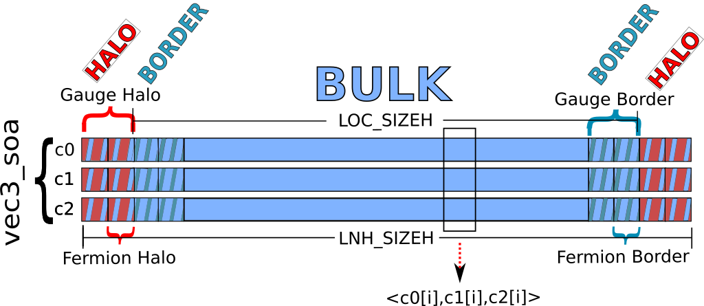
(a) The vec3_soa data structure

(b) The su3_soa data structure

Figure 1: Graphical view of how data structures corresponding to the vec3_soa and the su3_soa data-types are stored in memory. This layout allow to exploit instruction vectorization of the code.

4.2 The $D_{oe}$ and $D_{eo}$ operators

The application in the local domain of the $D_{oe}$ and $D_{eo}$ operators requires halos which are 1-site thick. Both functions are split into 3 pieces, two of which compute the result on the borders (using also data from the halos) and one computes the result on the bulk (which needs no data from the halos). After the computation ends, all halos must be updated: freshly computed data belonging to the borders must be sent to neighboring processes while new halo data must be retrieved from them. A schematic of this procedure is shown in Algorithm 1. The data to be transferred from and to each process in this case consists of 6 packets of size $8\leavevmode\nobreak\ n_{0,loc}n_{1,loc}n_{2,loc}$ bytes, as seen in Figure 1 (a typical size is around 250KB).

Algorithm 1 Parallelization of the $D_{oe}$ operator in our 1D-tiling approach (the $D_{eo}$ case is the same).

1:  $\phi^{(1)}_{o,l}=D_{oe,l}\phi^{(0)}_{e}$ on the lower border (on stream 1)

2:  $\phi^{(1)}_{o,u}=D_{oe,u}\phi^{(0)}_{e}$ on the upper border (on stream 2)

3:  $\phi^{(1)}_{o,b}=D_{oe,b}\phi^{(0)}_{e}$ in the bulk (on stream 3)

4:  Wait on stream 1 and 2

5:  Start asynchronous communications of fermion halos of $\phi^{(1)}_{o}$, that is $\phi^{(1)}_{o,l}$ and $\phi^{(1)}_{o,e}$ {6 send requests, 6 recv requests}

6:  Wait on stream 3 and on the 12 requests

4.3 The molecular dynamics evolution

For the pure gauge part of the molecular dynamics evolution, each iteration of the algorithm involves three steps: computing the forces from the gauge configuration at fictitious time $t$, evolving the momenta according to the evaluated forces to time $t+\delta t_{1}$, and finally evolving the gauge configuration to $t+\delta t_{2}$ (where $\delta t_{1}$ and $\delta t_{2}$ depend on the algorithm chosen). Notice that this is a constrained system. The first step is the only one that involves inter-process data moves: the so-called staples (which consist of products of all but one links along the perimeter of a rectangle) must be computed for $1\times 1$ and $1\times 2$ rectangles. For this step an update of the halos of the gauge configuration is required. The gauge configuration consists of 8 su3_soa structures depicted in Figure 1. The data to be transferred to and from each process consists of 96 packets, having size $8n_{0,loc}n_{1,loc}n_{2,loc}$ bytes (as in the case of the $D_{oe}$ and $D_{eo}$ operators). In order to allow for the superposition of communications of halos with computation in the bulk, we adopted the procedure described in Algorithm 2: all three steps are completed first on the borders, communications of the updated gauge configuration halos are started, the three steps are performed on the bulk, and then we wait for completion of all communication steps before starting the next iteration.

Algorithm 2 Parallelization of a block of pure-gauge molecular dynamics in our 1D-tiling approach.

1:  gauge force on the lower border

2:  gauge force on the upper border

3:  new momenta on the lower border

4:  new momenta on the upper border

5:  new configuration on the lower border

6:  new configuration on the upper border

7:  start asynchronous communications of new gauge configuration halos {96 send requests, 96 recv requests}

8:  force on the bulk

9:  new momenta on the bulk

10:  new configuration on the bulk

11:  Wait on the 192 requests

5 Performance results

In this section we initially describe the computing system we have used to run all the simulations, i.e. the COKA cluster, and then we analyze scaling and performance figures of the MPI-OpenACC application described in the previous sections.

In most Lattice QCD simulations one wants to complete a given number of Monte Carlo trajectories on a lattice of a specific size in the shortest possible time, so we focus on Strong Scaling, that is we analyze the compute time as a function of the number of compute devices used to solve the same problem size, as one splits the same lattice in smaller and smaller tiles. We study in larger details the two most time consuming phases of the code – the Dirac operator and the pure gauge molecular dynamics, describing their scaling behavior – but we also show performance results for the full code running on thermalized configurations with typical state-of-the-art physics parameters.

We analyze in finer details performance – and performance bottlenecks – for GPUs, since these processors have by far higher sustained performance than other architectures. However, since our code is fully portable to X86 CPUs we also show some results for them.

5.1 The COKA cluster

All our tests have been done on the COKA cluster, a GPU-based HPC cluster jointly operated by INFN and Università degli Studi di Ferrara, with a peak performance of $\approx 100$ TFLOPs.

The COKA cluster has 5 computing nodes, each node embedding $2\times$ Intel Xeon E5-2630v3 CPUs and $8\times$ NVIDA K80 dual-GPU boards. Each board hosts $2\times$ GK210 GPUs, so there are $16$ CUDA devices on each node. Nodes are interconnected with 56Gb/s FDR InfiniBand links; each node has $2\times$ Mellanox MT27500 Family [ConnectX-3] HCA, allowing multirail networking[46] for a doubled inter-node bandwidth. The two InfiniBand HCAs are connected respectively to the two PCIe root complexes, connected on their turn to the two CPU sockets. This allows for a symmetric hardware configuration, where each GPU has one local InfiniBand HCA, connected to the same PCIe root complex, so data messages do not need to traverse the inter-socket communication link (i.e. the Intel Quick Path Interconnect in this case). In all tests we have used the OpenMPI library, version 1.10.7, exploiting its CUDA-aware MPI capabilities, when running on GPUs.

5.2 The Dirac Operator

In this section we measure the Strong Scaling behavior and aggregate performance of the Dirac operator. We consider two different lattice sizes i.e. $32^{3}\times 48$ and $32^{3}\times 64$, which are relevant for physics simulations, and easily divisible across various numbers of GPUs. We split the former lattice on 1, 2, 4, 6, 8 and 12 GPUs, and the latter lattice on 2, 4, 8 and 16 GPUs.

As discussed in Sec. 3, this kernel scales perfectly as long as communication time is hidden by computing time over the bulk of the lattice. This is confirmed in Figure 2, where we can see a perfect Strong Scaling behavior up to $8$ GPUs for both lattice sizes. Further increasing the number of GPUs does not increase the performance anymore for the $32^{3}\times 48$ lattice, thus the speedup reaches a plateau. On the other hand, for the bigger $32^{3}\times 64$ lattice, using more than $8$ GPUs we can still have a performance increase, although using $16$ GPUs we are far from an optimal speedup.

Figure 2: Relative Speedup of the Dirac Operator in double precision on two lattices of size $32^{3}\times 48$ and $32^{3}\times 64$, for a growing number of GPUs hosted in the same compute node of the COKA Cluster.

To shed more light on this behavior we use the PGI Profiler to extract traces of the GPU kernel executions from an actual run of the code. From Figure 2, we know that for a lattice of $32^{3}\times 48$ sites the Dirac operator scales up to $8$ GPUs. Thus we profiled two different runs, using the same lattice size, and using respectively $8$ and $12$ GPUs, looking for execution differences which could explain the scaling impairment. Results are shown in Figure 3, clearly showing to which extent the computation phases overlap with communication in the two different cases.

(a) One iteration using $8$ GPUs. The time-lines of the kernels executing on two neighboring GPUs are shown, one over the other.

(b) One iteration using $12$ GPUs. The time-lines of the kernels executing on two neighboring GPUs are shown, one over the other.

Figure 3: Time-line of the execution of the Dirac operator on a lattice of $32^{3}\times 48$ sites using different numbers of GPUs ($8$ in Fig. 3a and $12$ in Fig. 3b). Purple-blue colored: execution of $D_{eo}$ and $D_{oe}$ on the borders of the lattice; turquoise colored: execution of $D_{eo}$ and $D_{oe}$ operations on the bulk of the lattice; gold colored: communication steps, as seen from the GPUs. Bulk operations are fully (3a) or partially (3b) overlapped with communication.

The Dirac Operator has 7 different kernels, shown in different colors and labeled in Figure 3a. The first three blocks on the left, acc_Doe_d3p, acc_Doe_d3m and acc_Doe_bulk, refer to the execution of the $D_{oe}$ kernel, respectively on the borders and on the bulk of the lattice, while acc_Deo_d3p, acc_Deo_d3m and acc_Deo_bulk, show $D_{eo}$, again on the borders and on the bulk of the lattice. Eventually, a final kernel, shown in red, is run for each iteration, performing just a zaxpy operation, corresponding to the final sum of Eq. 2.

Unlabeled yellow bars, represent MPI communications, as seen from the GPUs point of view; there are 6 communication steps for each iteration of $D_{eo}$ or $D_{oe}$, as expected. More interestingly, we can see that in Figure 3a communications are fully overlapped in time with the kernels operating on the bulk of the lattice. On the other hand, in Figure 3b, the execution time of those same kernels take a shorter amount of time, as we use a higher number of GPUs, so tiles are smaller. In the latter case, since communication time is approximately constant w.r.t. the tile size, the data transfer step is not completely hidden behind computation time on the bulk. This analysis (done on the actual code) fully explains the scalability limit displayed in Figure 2, since the overall execution time can not be decreased when communication time becomes the limiting factor.

From this analysis for the $32^{3}\times 48$ lattice, we obtain that we have a perfect Strong Scaling if lattice tiles associated to each GPU are at least $6$ sites thick, that is each GPU processes a $32^{3}\times 6$ slice of the lattice. This analysis also explains the behavior of the larger $32^{3}\times 64$ lattice in Figure 2: we should have a perfect Strong Scaling up to $10$ GPUs and then reach the plateau. As $64$ is not divisible by $10$ we cannot test precisely this configuration, but, using $16$ GPUs, we see a $10\times$ speedup, corresponding to the expected plateau figure.

In order to convert our scaling results into absolute performance figures, we have counted the floating point operations and memory accesses needed to apply the Dirac operator to each lattice site, directly accessing GPU hardware counters (through the PGI Profiler) and then double checking the results against theoretical expectations. From these measured values we have computed the actual sustained performance (floating point operations per second) and bandwidth (data bytes per second). This results are shown in Figure 4 for several runs using an increasing number of GPUs, on a $32^{3}\times 48$ lattice. Note that we include in our operation count the additional computational load associated to the data compression techniques that we have described in section 4.1.

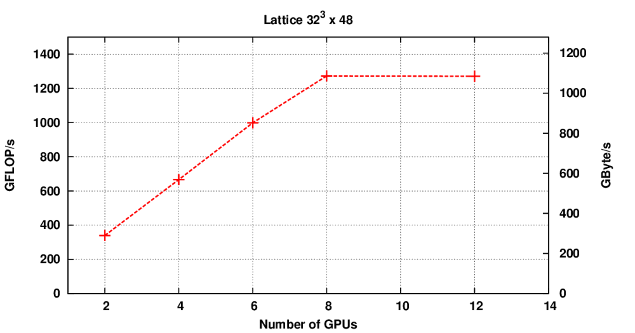
Figure 4: Aggregate performance (GFLOP/s) and bandwidth (Gbyte/s) for the Dirac operator om a $32^{3}\times 48$ lattice. Several runs of the same benchmark have been performed with different numbers of GPUs in the COKA Cluster.

As an example, using both GPUs of a NVIDIA K80 board, as shown in Figure 4, our implementation of the staggered Dirac Operator has a performance of $\simeq 339$ GFLOP/s in double precision and a sustained bandwidth of $\simeq 290$ GBytes/s (partially given also by cache accesses), that is $\approx 80\%$ of the aggregated raw peak memory bandwidth of the processor (taking into account the bandwidth penalty associated to Error-correcting-Codes (ECC) that we use throughout to increase data reliability). These figures are consistent with those obtained by other codes adopting non-portable architecture-specific languages[47].

5.3 Gauge part of the Molecular Dynamics

Figure 5: Relative speedup of the pure gauge part of the molecular dynamics kernel for two different lattices of size $32^{3}\times 48$ and $32^{3}\times 64$, as a function of the number of GPUs.

We now consider the Gauge part of the molecular dynamics, which is the second most time consuming step of the whole Monte Carlo code, after the Dirac operator.

As shown in Figure 5, for this phase of the simulation an almost perfect speedup can be appreciated up to $12$ and $16$ GPUs, respectively for the $32^{3}\times 48$ and the $32^{3}\times 64$ lattices (the same lattice sizes considered in Figure 2 for the Dirac operator). This different behavior can be explained by the fact that the computation-time versus communication-time ratio is more favorable in this case: to very first approximation, for each lattice site we use a data set which is $32$ times larger than for the Dirac operator, but the operation count increases by $\approx 300$. As a consequence, communications do not become the scaling limiting factor. Indeed, the true limiting factor encountered when increasing the number of compute devices (i.e. GPUs for this test), is the length of the tiling dimension. In fact, here lattice borders have a thickness of $2$ lattice sites, so Figure 5 shows an almost perfect scaling up to the point at which the bulk size reaches zero (since $48/12=64/16=4$) and the lattice cannot be further divided across more devices.

5.4 Full Simulation

To have a comprehensive view of the performance and scaling behavior of a complete run, as a representative example, we choose a simulation of QCD with 2 light (up and down) and 1 intermediate (strange) flavors over a $32^{3}\times 48$ lattice, that is part of a production run regarding the study of QCD at finite baryon density and towards the chiral limit. In this particular simulation (with quark mass $0.0015$ in lattice units and $\beta=3.3600$), the quark mass is about 1/3 of its physical value and the lattice spacing is around 0.3 fermi ($3\times 10^{-16}$ meters). For the computations in the molecular dynamics we are using floating-point operations, while for the Metropolis test we are using double-precision ones.

We have run the same simulation on different numbers of CPUs and GPUs available on the COKA cluster, demonstrating the actual code portability offered by the OpenACC programming model, and measuring performance. Our results are shown in Figure 6, as a function of the number of computing devices. We plot the aggregate performance (floating point operations per second) and aggregate Memory Bandwidth (data bytes per second). These metrics allow to appreciate both the strong scaling behavior and the differences in absolute performance between the two architectures.

Figure 6: Aggregate performance (GFLOP/s) and bandwidth (read/write GByte/s) for a full simulation on a $32^{3}\times 48$ lattice (see the text for a list of simulation parameters). The same simulation has been performed using different numbers of processors (CPUs or GPUs) in the COKA Cluster.

In Figure 6 we see that GPUs have much higher performance than CPUs for this kind of application. This was partly expected, since, when using just one processor, we had already measured a performance gap of approximately one order of magnitude[20]; this gap widens further when using multiple devices. As an example using two CPUs. execution times increases $\approx 14\times$ w.r.t. two GPUs. In order to put this figure in perspective, we note that the limitations of the compiler when targeting CPUs, that we had described in our previous work[20], still hold today; however, when using multiple devices, the performance measured on CPUs is further degraded by two main factors:

• The COKA cluster is a GPU dense machine, as each node hosts $16$ CUDA devices. This translates to the fact that all the GPU related points of Figure 6 are given by simulations executing on a single-node, without requiring inter-node communications, but only faster intra-node data transfers between GPU memories. On the other side, each node hosts only two CPUs, so CPU related points in Figure 6 refer to simulations run respectively on 1, 2, 3 and 4 nodes.

• When running on GPUs, communications can be overlapped with communications and small kernels (such as computations on the lattice borders) can run concurrently on the same device, as shown in Figure 3. On the other side, the current version of the PGI compiler completely ignores – when targeting CPUs – async clauses to OpenACC directives, and fully serialize the execution of different kernels and communications.

These factors can be, at least partially, overcome by: i) the use of CPU “denser” machines e.g. using CPUs with an higher core number or even Xeon Phi processors[48]; ii) the use of a compiler able to exploit the async OpenACC clause.

We also expect that single-CPU performance can be significantly increased, with improved data layouts. Remember that the data-layout chosen for this code (i.e. Structure of Array) allows code vectorization on both GPU and CPU architectures[44]; however, recent work[49, 48, 50] has shown that more complex data structures are able to increase the performance of memory sub-system performance on Intel CPUs and also Xeon-Phi accelerators. This has been demonstrated also for other lattice-based simulation codes[51].

We conclude at this stage that our code is actually portable to clusters adopting either Intel CPU or NVIDIA GPU architectures, but an additional effort is needed in the direction of performance portability, both on the programming side and on the side of improved compiler support for CPU architectures. In this latter regard we add that the community developing the GCC compiler seem to be strongly committed in supporting OpenACC and GCC, version 7, is expected to compile OpenACC codes for x86 CPU architecture.

6 Conclusions

In this work we have presented a full state-of-the-art production-grade code for Lattice QCD simulations with staggered fermions, coded using the OpenACC directive-based programming model to make the code portable across different computing architectures, and MPI to allow the code to run on multi-node systems where each node may have more then one accelerator installed.

This work extends the code we have developed in a previous work[20] designed to run on single-accelerator systems, turning it into a fully working MPI version able to exploit multi-node HPC clusters and multiple accelerators board within each computing node. We have described our implementation, detailing how parallelization has been exploited, and the strategies adopted to improve parallel efficiency, such as overlapping of MPI transfers with computation to hide communications time overheads. We have measured the scalability behavior of our code on the COKA GPU-based HPC cluster, and make also some tests on Intel CPU architectures. In this first implementation we have decides to use the 1d-tiling strategy, to keep the code structure simple, avoiding to handle non contiguous data communications, that for GPU-based clusters are not easily manageable[39], and also easily exploiting computation and communication overlap. As already commented in Sec. 3, this basic strategy keeps communication time constant while increasing the number of nodes, and for this reason the code scales as long as the communication time is hidden by the computation time.

In conclusion, our final result is a LQCD Monte Carlo code portable on a large subset of HPC clusters, based on both GPUs and standard CPUs, with satisfactory figures of aggregate performance and scalability. Performances measured on CPUs are lower compared with that of GPUs; this results is inline to what we have measured in our previous work, and the main reason is that the compiler does not fully yet support this architecture. We would like to highlight that this has not been a mere exercise on performance scalability: our efforts have been driven by the actual need to scale on multi-GPU architecture (basically for large RAM requirements) within the context of a project regarding QCD at finite baryon density, for which the present code has been already in full production since several months.

In the near future we plan to further optimize our code for Intel processors, without impacting the performance on NVIDIA GPUs, hoping for a contextual further development of the available compilers. We plan also to carefully assess the performance and scalability of our code on Intel KNL Xeon Phi clusters, as soon as the support for this architecture is added to the PGI compiler, or as soon as other compilers become available. On a longer time scale, we also plan to split the lattice across more dimensions and investigate the impact on performance, scalability and code maintainability, and to investigate the impact of different memory layout to improve vectorization of codes especially on multi-core CPUs.

References

- [1] A. Bazavov et al., Rev. Mod. Phys. 82, 1349 (2010), doi:10.1103/RevModPhys.82.1349.
- [2] Z. Fodor and C. Hoelbling, Rev. Mod. Phys. 84, p. 449 (2012), doi:10.1103/RevModPhys.84.449.
- [3] H.-T. Ding, F. Karsch and S. Mukherjee, Thermodynamics of Strong-Interaction Matter from Lattice QCD, in Quark-Gluon Plasma 5, ed. X.-N. Wang 2016, pp. 1–65. doi:10.1142/9789814663717_0001.
- [4] G. Aarts, J. Phys. Conf. Ser. 706, p. 022004 (2016), doi:10.1088/1742-6596/706/2/022004.
- [5] A. Kennedy, arXiv preprint hep-lat/0607038 (2006).
- [6] C. Bernard, N. Christ, S. Gottlieb, K. Jansen, R. Kenway, T. Lippert, M. Lüscher, P. Mackenzie, F. Niedermayer, S. Sharpe, R. Tripiccione, A. Ukawa and H. Wittig, Nuclear Physics B - Proceedings Supplements 106-107, 199 (2002), doi:https://doi.org/10.1016/S0920-5632(01)01664-4.
- [7] G. Bilardi, A. Pietracaprina, G. Pucci, F. Schifano and R. Tripiccione, Lecture Notes in Computer Science 3769, 386 (2005), doi:10.1007/11602569_41.
- [8] M. Albanese et al., Comput. Phys. Commun. 45, 345 (1987), doi:10.1016/0010-4655(87)90172-X.
- [9] P. A. Boyle, D. Chen, N. H. Christ, M. A. Clark, S. D. Cohen, C. Cristian, Z. Dong, A. Gara, B. Joo, C. Jung, C. Kim, L. A. Levkova, X. Liao, G. Liu, R. D. Mawhinney, S. Ohta, K. Petrov, T. Wettig and A. Yamaguchi, IBM Journal of Research and Development 49, 351 (March 2005), doi:10.1147/rd.492.0351.
- [10] F. Belletti, S. F. Schifano, R. Tripiccione, F. Bodin, P. Boucaud, J. Micheli, O. Pene, N. Cabibbo, S. De Luca, A. Lonardo, D. Rossetti, P. Vicini, M. Lukyanov, L. Morin, N. Paschedag, H. Simma, V. Morenas, D. Pleiter and F. Rapuano, Computing in Science and Engineering 8, 50 (2006), doi:10.1109/MCSE.2006.4.
- [11] N. R. Adiga et al., An Overview of the BlueGene/L Supercomputer, in Supercomputing, ACM/IEEE 2002 Conference, Nov 2002. doi:10.1109/SC.2002.10017.
- [12] G. Goldrian, T. Huth, B. Krill, J. Lauritsen, H. Schick, I. Ouda, S. Heybrock, D. Hierl, T. Maurer, N. Meyer, A. Schaefer, S. Solbrig, T. Streuer, T. Wettig, D. Pleiter, K.-H. Sulanke, F. Winter, H. Simma, S. Schifano, R. Tripiccione, A. Nobile, M. Drochner, T. Lippert and Z. Fodor, Computing in Science and Engineering 10, 46 (2008), doi:10.1109/MCSE.2008.153.
- [13] R. Haring, M. Ohmacht, T. Fox, M. Gschwind, D. Satterfield, K. Sugavanam, P. Coteus, P. Heidelberger, M. Blumrich, R. Wisniewski, a. gara, G. Chiu, P. Boyle, N. Chist and C. Kim, IEEE Micro 32, 48 (March 2012), doi:10.1109/MM.2011.108.
- [14] OpenACC directives for accelerators http://www.openacc-standard.org/.
- [15] The OpenMP API specification for parallel programming http://www.openmp.org/specifications/.
- [16] S. Blair, C. Albing, A. Grund and A. Jocksch, Accelerating an mpi lattice boltzmann code using openacc, in Proceedings of the Second Workshop on Accelerator Programming Using Directives, WACCPD ’15 (ACM, New York, NY, USA, 2015). doi:10.1145/2832105.2832111.
- [17] J. Kraus, M. Schlottke, A. Adinetz and D. Pleiter, Accelerating a c++ cfd code with openacc, in Accelerator Programming using Directives (WACCPD), 2014 First Workshop on, 2014. doi:10.1109/WACCPD.2014.11.
- [18] E. Calore, A. Gabbana, J. Kraus, S. F. Schifano and R. Tripiccione, Concurrency and Computation: Practice and Experience 28, 3485 (2016), doi:10.1002/cpe.3862.
- [19] S. Gupta and P. Majumdar, ArXiv e-prints (October 2017), arXiv:1710.09178.
- [20] C. Bonati, S. Coscetti, M. D’Elia, M. Mesiti, F. Negro, E. Calore, S. F. Schifano, G. Silvi and R. Tripiccione, International Journal of Modern Physics C 28 (2017), doi:10.1142/S0129183117500632.
- [21] C. Bonati, G. Cossu, M. D’Elia and P. Incardona, Comput. Phys. Commun. 183, 853 (2012), doi:10.1016/j.cpc.2011.12.011.
- [22] H. J. Rothe, Lattice gauge theories. An Introduction. (World Scientific, 2005).
- [23] T. DeGrand and C. DeTar, Lattice methods for quantum chromodynamics (World Scientific, 2006).
- [24] P. Weisz, Nuclear Physics B 212, 1 (1983).
- [25] G. Curci, P. Menotti and G. Paffuti, Physics Letters B 130, 205 (1983).
- [26] C. Morningstar and M. Peardon, Physical Review D 69, p. 054501 (2004).
- [27] T. A. Degrand and P. Rossi, Computer Physics Communications 60, 211 (1990), doi:http://dx.doi.org/10.1016/0010-4655(90)90006-M.
- [28] M. Clark, A. Kennedy and Z. Sroczynski, arXiv (2004), hep-lat/0409133.
- [29] M. Clark and A. Kennedy, Physical review letters 98, p. 051601 (2007).
- [30] M. Clark and A. Kennedy, Physical Review D 75, p. 011502 (2007).
- [31] S. Duane, A. D. Kennedy, B. J. Pendleton and D. Roweth, Physics letters B 195, 216 (1987).
- [32] B. Jegerlehner, arXiv (1996), hep-lat/9612014.
- [33] V. Simoncini and D. B. Szyld, Numerical Linear Algebra with Applications 14, 1 (2007).
- [34] J. Sexton and D. Weingarten, Nuclear Physics B 380, 665 (1992).
- [35] C. Urbach, K. Jansen, A. Shindler and U. Wenger, Computer Physics Communications 174, 87 (2006).
- [36] I. Omelyan, I. Mryglod and R. Folk, Physical Review E 65, p. 056706 (2002).
- [37] I. Omelyan, I. Mryglod and R. Folk, Computer Physics Communications 151, 272 (2003).
- [38] T. Takaishi and P. De Forcrand, Physical Review E 73, p. 036706 (2006).
- [39] E. Calore, A. Gabbana, J. Kraus, E. Pellegrini, S. F. Schifano and R. Tripiccione, Parallel Computing 58, 1 (2016), doi:10.1016/j.parco.2016.08.005.
- [40] E. Calore, D. Marchi, S. F. Schifano and R. Tripiccione, Optimizing communications in multi-GPU Lattice Boltzmann simulations, in High Performance Computing Simulation (HPCS), 2015 International Conference on, July 2015. doi:10.1109/HPCSim.2015.7237021.
-
[41]
An Introduction to CUDA-Aware MPI
http://developer.nvidia.com/content/introduction-cuda-aware-mpi. -
[42]
Benchmarking GPUDirect RDMA on modern server platforms
http://devblogs.nvidia.com/parallelforall/benchmarking-gpudirect-rdma-on-modern-server-platforms. - [43] S. Wienke, C. Terboven, J. Beyer and M. Müller, LNCS 8632, 812 (2014), doi:10.1007/978-3-319-09873-9_68.
- [44] C. Bonati, E. Calore, S. Coscetti, M. D’Elia, M. Mesiti, F. Negro, S. F. Schifano and R. Tripiccione, Development of scientific software for HPC architectures using OpenACC: the case of LQCD, in The 2015 International Workshop on Software Engineering for High Performance Computing in Science (SE4HPCS), ICSE Companion Proceedings2015. doi:10.1109/SE4HPCS.2015.9.
- [45] J. D. McCalpin, IEEE Technical Committee on Computer Architecture (TCCA) Newsletter (Dec 1995).
- [46] J. Liu, A. Vishnu and D. K. Panda, Building multirail InfiniBand clusters: MPI-level design and performance evaluation, in Proceedings of the 2004 ACM/IEEE conference on Supercomputing, 2004.
- [47] R. Li, C. DeTar, S. Gottlieb and D. Toussaint, ArXiv e-prints (November 2017), arXiv:1712.00143.
- [48] I. Kanamori and H. Matsufuru, ArXiv (December 2017), arXiv:1712.01505.
- [49] J. Jeffers, J. Reinders and A. Sodani, Chapter 26 - Quantum Chromodynamics, in Intel Xeon Phi Processor High Performance Programming, eds. J. Jeffers, J. Reinders and A. Sodani (Morgan Kaufmann, Boston, 2016), pp. 581 – 598, Second edn. doi:10.1016/B978-0-12-809194-4.00026-0.
- [50] B. Joó, M. Smelyanskiy, D. D. Kalamkar and K. Vaidyanathan, Chapter 9 - wilson dslash kernel from lattice QCD optimization, in High Performance Parallelism Pearls, eds. J. Reinders, and J. Jeffers (Morgan Kaufmann, Boston, 2015), pp. 139 – 170. doi:https://doi.org/10.1016/B978-0-12-803819-2.00023-9.
- [51] E. Calore, A. Gabbana, S. F. Schifano and R. Tripiccione, The International Journal of High Performance Computing Applications , 1 (2017), doi:10.1177/1094342017703771.