Cluster-weighted latent class modeling

Usually in Latent Class Analysis (LCA), external predictors are taken to be cluster conditional probability predictors (LC models with covariates), and/or score conditional probability predictors (LC regression models). In such cases, their distribution is not of interest. Class specific distribution is of interest in the distal outcome model, when the distribution of the external variable(s) is assumed to dependent on LC membership. In this paper, we consider a more general formulation, typical in cluster-weighted models, which embeds both the latent class regression and the distal outcome models. This allows us to test simultaneously both whether the distribution of the covariate(s) differs across classes, and whether there are significant direct effects of the covariate(s) on the indicators, by including most of the information about the covariate(s) - latent variable relationship. We show the advantages of the proposed modeling approach through a set of population studies and an empirical application on assets ownership of Italian households.

Key-Words: latent class analysis, latent class regression models, continuous distal outcomes, direct effects, cluster-weighted models, household wealth, assets ownership

1 Introduction

Latent class analysis (McCutcheon, 1985) is widely used in the social and behavioral sciences to locate subgroups of observations in the sample based on a set of $J$ observed response variables $\mathbf{Y}$. Examples of applications include identification of types of mobile internet usage in travel planning and execution (Okazaki ., 2015), types of political involvement (Hagenaars  Halman, 1989), classes of treatment engagement in adolescents with psychiatric problems (Roedelof ., 2013), a typology of infant temperament (Loken, 2004), modeling phases in the development of transitive reasoning (Bouwmeester  Sijtsma, 2007), or classes of self disclosure (Maij-de Meij ., 2005).

In many empirical studies, interest lies in investigating which external variables $\mathbf{Z}$ predict latent class membership $X$. Latent class models with covariates (Dayton  Macready, 1988) are a well-known extension of the baseline model, in which external variables are included in the latent class modeling framework as predictors of class membership (Collins  Lanza, 2010). Stegmann  Grimm (2017), for instance, discuss the inclusion of covariates in more complicated LC models. However, recent methodological development has shifted the attention towards modeling the effect in the opposite direction. That is, predicting a - possibly continuous - distal outcome based on the latent class membership (Bakk ., 2013; Lanza ., 2013), as depicted in Figure 1. Although there can be more than one external variable available, for sake of exposition here we describe the models with only one external variable.

Figure 1: Latent class model with distal outcome.

For instance, Roberts  Ward (2011) predict distal pain outcomes based on class memberships defined by patterns of barriers to pain management and Mulder . (2012) compared average measures of recidivism in clusters of juvenile offenders.

Typically, in distal outcome models, the distal outcome and the $J$ response variables $\mathbf{Y}$’s are assumed to be conditionally independent given the latent variable $X$ (Bakk ., 2013; Lanza ., 2013). A direct effect of $Z$ on $\mathbf{Y}$ is therefore not allowed for, neither its presence tested. In latent variable modeling, it is well known that Maximum Likelihood (ML) estimation is subject to severe bias when direct effects are present in LC and latent trait models (Asparouhov  Muthén, 2014, regression mixture models (Kim ., 2016; Nylund-Gibson  Masyn, 2016), and latent Markov models (Di Mari  Bakk, 2017), and are not accounted for.

Given the restrictiveness of the conditional independence assumption and the possible severity of its violation, we propose a more general model that can account for complex interdependencies between the external variable, LC membership, and the indicators of the LC model. In regression mixtures, a “circular” relation among $\mathbf{Y}$-$X$-$Z$ is commonly considered in the cluster-weighted modeling approach (Ingrassia ., 2012, 2014, 2015; Punzo, 2014; Dang ., 2017). That is, a more general model is specified, where next to modeling the class specific distribution of $Z$ (distal outcome situation), also the direct effect of $Z$ on $\mathbf{Y}$ is modeled (latent class regression). If $\mathbf{Y}$ are indicators of assets ownership, and $Z$ is a measure (in euro) of net (of liabilities) wealth, the cluster-weighted modeling approach allows net wealth also to directly affect a household decision to own assets. With standard inference, the statistical significance of each effect can then be tested to see whether intermediate model specifications are more appropriate.

In LC regression models (Kamakura  Russel, 1989; Wedel  DeSarbo, 1994), although the assumption of conditional independence of $\mathbf{Y}$ and $Z$ can be relaxed (see Figure 2), the distal outcome’s distribution is not of interest and hence not modeled. Therefore, in the traditional LCA approach, an external variable enters the model either as a covariate (latent class regression) or as a distal outcome, but never as both at the same time. We propose to extend the idea of cluster-weighted modeling in the context of latent class analysis, by proposing a generalized version of the models in Figures 1 and 2, as depicted in Figure 3, which embeds them both.

Figure 2: Latent class regression model.

Figure 3: Latent class cluster-weighted model.

By starting from the most general model, the user can proceed backwards, testing the model assumptions of both the distal outcome and the latent class regression models. In particular, in this paper we will show evidence, based on a set of population studies and an empirical application, that 1) if direct effects are present, our approach, contrary to the distal outcome model, yields unbiased estimates of the distal outcome cluster specific means and variances; and 2) if the most suitable model is one between the distal outcome model or the latent class regression model, the relative class sizes and compositions will be the same as the ones delivered under the proposed modeling approach.

The paper proceeds as follows. In Section 2, we illustrate the proposed modeling approach through three population studies, in comparison with the LC regression and the distal outcome models. We give model definitions and details on the parameterizations in Section 3. In Section 4, we analyze data from the Household Finance and Consumption Survey, and conclude with some final remarks in Section 5.

2 Population studies

This Section is devoted to showing very simple and intuitive evidence, obtained by analyzing three large data sets (30000 sample units) - each drawn from the three models in Figures 1, 2 and 3 - in order to motivate the application of the cluster-weighted modeling approach in LCA (see Table 1). We set the number of latent classes $S=2,$ and to begin with we fit all three models assuming this value to be known. At the end of the Section, we will also show results on estimation of the number of latent classes based on BIC.

		Acronym	Data
Latent Class regression		LCreg	LCreg
Latent Class with distal outcome		LCdist	LCdist
Latent Class cluster-weighted		LCcw	LCcw

Table 1: Legend of acronyms used for the population models and for the generated data.

To get approximately equal (realistic) conditions on class separation, we generated the data such that the entropy-based $R^{2}$ (Magidson, 1981) for the correctly specified model is about 0.7 in all the three data sets - which is the minimum class separation to get a good LC model (Vermunt, 2010; Asparouhov  Muthén, 2014). The data were generated in R (R Core Team, 2017), and parameter estimation was carried out with Latent GOLD 5.1 (Vermunt  Magidson, 2016).

2.1 LCreg data

The LCreg data set was generated from a two-class LCreg model, with class memberships of 0.7 and 0.3, six dichotomous indicators $(J=6)$ and one continuous $Z$ - drawn from a standard normal distribution - loaded on all six indicators. The external variable $Z$ is loaded on the indicators with a coefficient of -0.5, if the most likely response is on the first class, or 1, if the most likely response is on the second class, giving a large effect size.

	Class proportions			Entr. $R^{2}$		#par
LCreg	0.7010	0.2990		0.7675		25
LCdist	0.7357	0.2643		0.8639		17
LCcw	0.7018	0.2982		0.7681		29

Table 2: LCreg data. Estimated class proportions, entropy-based $R^{2}$ and number of parameters for each of the three estimated models. Results from correctly specified model in bold font.

We observe in Table 2 that the LCdist model overinflates the mixing proportion on the bigger class, whereas the LCcw model yields nearly equivalent class proportions as in the correctly specified case. This at the cost of four more parameters to be estimated.

Table 3 reports estimated means and variances for the variable $Z$ based on the LCdist and LCcw models, along with standard errors and $p$-values of the Wald tests of equality of the means and the variances. Nothing is reported for LCreg, as $Z$ is not modeled. In the LCdist model, both the means are wrongly estimated to be statistically different from zero. Moreover, based on the reported Wald tests, we reject the nulls of equal means and equal variances (with $p$-values smaller than 0.01). These findings for the LCdist model can be explained by the fact that it wrongly predicts a clustered distribution on $Z$ in order to accommodate for a direct effect of $Z$ on the indicators which is not accounted for. This creates an additional source of entropy in the class solution (as displayed by the relatively higher value of the entropy-based $R^{2}$).

	Means		Wald(=) $p$	Variances		Wald(=) $p$
LCdist	0.0525***	-0.1640***	0.0000	1.0301	0.8846	0.0000
	(0.0071)	(0.0122)		(0.0100)	(0.0158)
LCcw	-0.0010	-0.0134	0.9000	0.9966	1.0105	0.6100
	(0.0086)	(0,0163)		(0.0114)	(0.0208)

Table 3: LCreg data. Estimated means (*** $p$-value$<$0.01, ** $p$-value$<$0.05, * $p$-value$<$0.1) and variances , and $p$-values from Wald test of equality of component means and variances for the LCdist model and the LCcw model. Standard errors in parentheses.

2.2 LCdist data

The LCdist data set was generated from a two-class LCdist model, with class memberships of 0.7 and 0.3, six dichotomous indicators ($J=6$) and one continuous $Z$, drawn from a mixture of two normal distributions with means of -1 and 1 and common variance of 1.

	Class proportions			Entr. $R^{2}$		#par
LCreg	0.5850	0.4150		0.2781		25
LCdist	0.7006	0.2994		0.7274		17
LCcw	0.7026	0.2974		0.7320		29

Table 4: LCdist data. Estimated class proportions, entropy $R^{2}$ and number of parameters for each of the three estimated models. Results from correctly specified model in bold font.

The LCreg model yields a completely distorted class solution, whereby both the LCdist and LCcw models yields almost identical (correct) solutions (Table 4).

Interestingly, the misspecified response-$Z$ relation in the LCreg model yields a solution with relatively smaller class separation (as measured by the entropy-based $R^{2}$).

Next, we compare estimates of class-specific means and variances of $Z$ as obtained by the LCdist and LCcw models.

	Means		Wald(=) $p$	Variances		Wald(=) $p$
LCdist	-0.9911***	1.0156***	0.0000	1.0072	0.9886	0.4000
	(0.0084)	(0.0145)		(0.0119)	(0.0196)
LCcw	-0.9889***	1.0242***	0.0000	1.0075	0.9810	0.2700
	(0.0096)	(0,0176)		(0.0125)	(0.0207)

Table 5: LCdist data. Estimated means (*** $p$-value$<$0.01, ** $p$-value$<$0.05, * $p$-value$<$0.1) and variances , and $p$-values from Wald test of equality of component means and variances for the LCdist model and the LCcw model. Standard errors in parentheses. Results from correctly specified model in bold font.

The LCdist and the LCcw models estimate almost identical means and variances of $Z$, both correctly not rejecting the null of common variance across latent classes. We observe that the SE’s for the less parsimonious LCcw model are systematically larger than those of the correctly specified model: this is not surprising, as having less degrees of freedom corresponds, all else equal, to slightly more variable estimates.

2.3 LCcw data

The LCcw data was generated from a two-class LCcw model, with class memberships of 0.7 and 0.3, six dichotomous indicators ($J=6$) and one continuous $Z$, drawn from a mixture of two normal distributions with means of -1 and 1 and common variance of 1.

	Class proportions			Entr. $R^{2}$		#par
LCreg	0.8899	0.1101		0.5611		25
LCdist	0.4373	0.5627		0.6441		17
LCcw	0.6993	0.3007		0.7045		29

Table 6: LCcw data. Estimated class proportions, entropy-based $R^{2}$ and number of parameters for each of the three estimated models. Results from correctly specified model in bold font.

Both the LCreg and the LCdist models deliver distorted class solutions (Table 6). Although with a higher entropy-based $R^{2},$ the residual dependence among the indicators due to the exclusion of the direct effect causes a more severe distortion in the LCdist model compared to the LCreg model. Equally we observe (Table 7) that the means and variance(s) of $Z$ are both biased in the LCdist model. Contrary to the correctly specified model, in LCdist the Wald test cannot reject the equal variances hypothesis (at 1 % level).

	Means		Wald(=) $p$	Variances		Wald(=) $p$
LCdist	-1.4544***	0.4159***	0.0000	0.7044	1.2096	0.0000
	(0.0102)	(0.0120)		(0.0111)	(0.0159)
LCcw	-1.0029***	0.9955***	0.0000	1.0215	0.9818	0.0380
	(0.0104)	(0,0122)		(0.0146)	(0.0160)

Table 7: LCcw data. Estimated means (*** $p$-value$<$0.01, ** $p$-value$<$0.05, * $p$-value$<$0.1) and variances , and $p$-values from Wald test of equality of component means and variances for the LCdist model and the LCcw model. Standard errors in parentheses. Results from correctly specified model in bold font.

Table 8 reports adjusted Rand indexes ARI (Hubert  Arabie, 1985), arranged in a three-by-three table, comparing the hard partitions obtained with each fitted model under the three data generating model scenarios. The results are in line with what observed above. When the data are generated with a LCreg model, the LCcw model delivers an almost identical partition to that of the correctly specified model, followed close up by the LCdist model - with only about 3% difference. In the LCdist data set as well, the LCcw model’s partition is nearly as in the correctly specified model (ARI of $\approx 0.99$), whereby the ARI drops to $\approx 0.21$ when the comparison is with the LCreg partition. In the latest scenario - LCcw data set - fitting both the LCreg and the LCdist models delivers in both cases quite different partitions ($\approx 0.16$ and $\approx 0.31$ ARI’s) compared to the correctly specified model.

			Fitted model
Data		Correct model	LCreg	LCdist	LCcwm
LCreg		LCreg	1	0.9732	0.9997
LCdist		LCdist	0.2125	1	0.9889
LCcw		LCcw	0.1604	0.3101	1

Table 8: Adjusted Rand indexes, computed between clustering with correctly specified models - LCreg, LCdist and LCcw models - and clustering with the other two models

Based on the above data sets, in Table 9 we report also results on BIC values for the three models in all three scenarios, for $S=1,\dots,5$. Although BIC values can be compared for LCdist and LCcw, selecting a model among the three with BIC cannot be done as $Z$ in LCreg is not modeled and the model likelihoods are therefore not comparable. In both the LCreg and LCdist data sets, BIC for the LCcw model selects, together with the correctly specified model in the first two scenarios, the correct number of classes. Interestingly however, misspecifying the indicators-$Z$ relation causes, in both the LCreg and LCdist models, a severe overstatement of the number of classes (LCcw data set).

			Number of components
Data			$S=1$	$S=2$	$S=3$	$S=4$	$S=5$
LCreg $\begin{dcases*}\\ \\ \end{dcases*}$		LCreg	235957.23	191309.94	191411.62	191539.73	191642.90
		LCdist	321109.39	283926.34	278042.32	277453.71	277117.53
		LCcw	321137.31	276509.33	276636.54	276766.45	276888.98
LCdist $\begin{dcases*}\\ \\ \end{dcases*}$		LCreg	233652.06	231508.46	231251.75	231041.07	230893.17
		LCdist	348714.25	331953.90	332037.14	332112.24	332189.69
		LCcw	337204.58	332067.91	332198.43	332329.23	332449.70
LCcw $\begin{dcases*}\\ \\ \end{dcases*}$		LCreg	213395.81	207054.91	206149.45	205996.43	205922.50
		LCdist	321792.35	310231.51	306431.47	305466.02	304613.18
		LCcw	316998.91	303623.67	303759.81	303910.04	304025.80

Table 9: Model selection with BIC computed for each model at each data generating model - LCreg, LCdist and LCcw models - for $S=1,\dots,5$. Data generating model and minimum BIC value, for each model at each scenario, in bold.

3 The different modeling approaches in details

3.1 The latent class cluster-weighted model

Let $\operatorname{\mathbf{Y}}=(Y_{1},\dots,Y_{J})^{\prime}$ be the vector of the full response pattern and $\operatorname{\mathbf{y}}$ its realization. Let us assume also one continuous external variable $Z$ is available, and we denote as $z$ its realization. Let us denote as $X$ the categorical latent variable, with latent classes $s=1,\dots,S.$ A general form of association between $\operatorname{\mathbf{Y}},$ $X$ and $Z,$ involves modeling the following joint probability

$$P(Z=z,X=s,\operatorname{\mathbf{Y}}=\operatorname{\mathbf{y}})=P(Z=z,X=s)P(\operatorname{\mathbf{Y}}=\operatorname{\mathbf{y}}|Z=z,X=s),$$ (1)

where the common assumption in LCA of $\operatorname{\mathbf{Y}}$ and $Z$ being conditionally independent given the latent process is relaxed. From Equation (1), several submodels can be specified (covariate model, distal outcome model, etc). If substantive theoretical arguments postulate the latent variable to be a predictor of the external variable $Z,$ the latent class cluster-weighted model specifies the probability of observing a response pattern $\operatorname{\mathbf{y}}$ as

$$P(\operatorname{\mathbf{Y}}=\operatorname{\mathbf{y}},Z=z)=\sum_{s=1}^{S}\underbrace{P(X=s)}_{\text{a}}\underbrace{P(Z=z|X=s)}_{\text{b}}\underbrace{P(\operatorname{\mathbf{Y}}=\operatorname{\mathbf{y}}|Z=z,X=s)}_{\text{c}},$$ (2)

which is defined by three components: the structural component (a), which describes the latent class variable, a measurement component (b), connecting the latent class to the observed responses with a direct effect of $Z$, and the external variable model (c), which models the latent class specific distribution of $Z$. Under the assumption of local independence of response variables given the class membership and $Z$, the conditional distribution of the responses can be written as

$$P(\operatorname{\mathbf{Y}}=\operatorname{\mathbf{y}}|Z=z,X=s)=\prod_{j=1}^{J}P(Y_{j}=y_{j}|Z=z,X=s).$$ (3)

For estimating the model in Equation (2), we assume each $Y_{j}$ to be conditionally Bernoulli distributed, with success probability $\pi_{sj},$ and parametrize the conditional response probabilities through the following log-odds

$$\log\left(\frac{\pi_{js}}{1-\pi_{js}}\right)=\beta_{0,js}+Z\beta_{js},$$ (4)

whereby $Z$ is assumed to be conditionally Gaussian with mean $\mu_{s}$ and variance $\sigma^{2}_{s},$ for $1\leq s\leq S.$

The model of Equation (2) can be used to assign observations to clusters based on the posterior membership probabilities

$$P(\text{X}=s|\operatorname{\mathbf{Y}}=\mathbf{y},Z=z)=\frac{P(X=s)P(Z=z|X=s)P(\operatorname{\mathbf{Y}}=\operatorname{\mathbf{y}}|Z=z,X=s)}{P(\operatorname{\mathbf{Y}}=\operatorname{\mathbf{y}},Z=z)},$$ (5)

according to, for instance, modal or proportional assignment rules.

The latent class unconditional probabilities can as well be parametrized using logistic regressions. We opt for the following parametrization

$$\log\left(\frac{P(X=s)}{P(X=1)}\right)=\theta_{s},$$ (6)

for $1<s\leq S,$ where we take the first category as reference, and we set to zero the related parameter. The total number of free parameters to be estimated is therefore $2(J\times S)$ for the measurement model, $2S$ for the external variable model, and $S-1$ for the structural model.

Notice that, by setting the $\beta_{js}$’s of Equation (4) to zero, the LC cluster-weighted model reduces to a standard LC with distal outcome model. By contrast, given that the external variable component is completely missing, the LC regression is not formally nested in the LC cluster-weighted model, although it can be thought of as a sub-model in which the conditional distribution of $\mathbf{Y}|Z$ is modeled, and $Z$ is taken as fixed-value rather than a random variable to be modeled as well.

3.2 The LC with distal outcome model

It is common, in LCA, to consider a less general version of the joint distribution of Equation (1), by assuming the responses and $Z$ to be conditionally independent given the latent process. If, again, the latent class variable is taken to be a predictor of the external variable $Z,$ this yields the following latent class with distal outcome model

$$P(\operatorname{\mathbf{Y}}=\operatorname{\mathbf{y}},Z=z)=\sum_{s=1}^{S}P(X=s)P(Z=z|X=s)P(\operatorname{\mathbf{Y}}=\operatorname{\mathbf{y}}|X=s).$$ (7)

Under the local independence assumption of the items given the latent class variable, the response conditional probabilities can be written, similarly to Equation (3), as

$$P(\operatorname{\mathbf{Y}}=\operatorname{\mathbf{y}}|X=s)=\prod_{j=1}^{J}P(Y_{j}=y_{j}|X=s),$$ (8)

and parametrized through the following log-odds

$$\log\left(\frac{\pi_{js}}{1-\pi_{js}}\right)=\beta_{0,js}.$$ (9)

The model of Equation (7) can be used to cluster observations, according to modal or proportional assignment rules, based on the following posterior membership probabilities

$$P(\text{X}=s|\operatorname{\mathbf{Y}}=\mathbf{y},Z=z)=\frac{P(X=s)P(Z=z|X=s)P(\operatorname{\mathbf{Y}}=\operatorname{\mathbf{y}}|X=s)}{P(\operatorname{\mathbf{Y}}=\operatorname{\mathbf{y}},Z=z)}.$$ (10)

The external variable $Z$ is assumed, conditional to the latent class, to be Gaussian with mean $\mu_{s}$ and variance $\sigma^{2}_{s},$ for $1\leq s\leq S,$ whereby the latent class unconditional probabilities are parametrized as in Equation (6). This yields $J\times S+2S+S-1$ free parameters to be estimated. The only difference with the model of Equation (2) is that $\mathbf{Y},$ in the measurement component, is conditional only on $X$, not on $Z$. That is, $\mathbf{Y}$ is assumed to be independent of $Z$ given $X$, which is a standard, and rather very strong, assumption of LCA.

3.3 The LC regression model

Rather than modeling the joint distribution $P(Z,X,\operatorname{\mathbf{Y}})$ of Equation (1), the latent class regression models the conditional distribution of $\operatorname{\mathbf{Y}}$ given $Z$ and the latent class variable, specifying the following model for $\operatorname{\mathbf{Y}}$:

$$P(\operatorname{\mathbf{Y}}=\operatorname{\mathbf{y}}|Z=z)=\sum_{s=1}^{S}P(X=s)P(\operatorname{\mathbf{Y}}=\operatorname{\mathbf{y}}|Z=z,X=s).$$ (11)

In this case, the conditional response probabilities depend on the external variable $Z$ and, under local independence of the responses given the latent variable, the measurement model can be written as in Equation (3), and parametrized as in Equation (4). The posterior membership probabilities, computed based on the model in Equation (11), are as follows

$$P(\text{X}=s|\operatorname{\mathbf{Y}}=\mathbf{y},Z=z)=\frac{P(X=s)P(Z=z|X=s)P(\operatorname{\mathbf{Y}}=\operatorname{\mathbf{y}}|X=s)}{P(\operatorname{\mathbf{Y}}=\operatorname{\mathbf{y}},Z=z)}.$$ (12)

With latent class unconditional probabilities parametrized as in Equation (6), the total number of free parameters to be estimated is $2(J\times S)+S-1.$

		Dir. Eff.	$Z$ modeled	#par
Latent Class regression		$\checkmark$	$\times$	$2(J\times S)+(S-1)$
Latent Class with distal outcome		$\times$	$\checkmark$	$(J\times S)+2S+(S-1)$
Latent Class cluster-weighted		$\checkmark$	$\checkmark$	$2(J\times S)+2S+(S-1)$

Table 10: Summary of different modeling assumptions and number of free parameters to be estimated.

Table 10 summarizes how $Z$ enters each of the three models, and the total number of free parameters to be estimated. Intuitively, this shows that the first two models can be seen as special cases of the third model, which therefore models the relationship between the 3 sets of variables in the most exhaustive manner.

4 A latent class model of households’ assets ownership to predict wealth

Household wealth cannot be directly observed. Nonetheless, measuring it is a crucial issue for any policy maker. Notably, survey measures of income - or expenditure, if available - are affected by substantial measurement error and systematic reporting bias (Ferguson ., 2003; Moore  Welniak, 2000). In addition, if wealth as a measure of permanent income (Friedman, 1957) is of interest, current income, even if measured without error, is likely to be a poor approximation. In more recent surveys (like the Household Finance and Consumption Survey, from the European Central Bank), a measure of net wealth - value of total household assets minus the value of total liabilities - is provided. However, relying on each household’s subjective evaluation of the current value of each asset they own, such a measure is prone to considerable measurement error as well. Furthermore, having such a complex measure is complicated to understand for a more general audience, to whom a simpler classification/index would appeal.

Latent Trait (LTA) and Latent Class Analysis have been used in order to model wealth - or, inversely, deprivation - from observed assets ownership. Whereby in the LTA framework, wealth is modeled as a continuous trait (Szeles  Fusco, 2013; Vandemoortele, 2014), LCA was used (Moisio, 2004; Pérez-Mayo, 2005) based on the idea that wealth (poverty) can be seen as a multidimensional latent construct. Although determining which ownership indicators to use can be a problem, arguably they all attempt to identify subgroups in the population based on the same multidimensional phenomenon (Moisio, 2004): different dimensions of wealth are measured by different (sets of) indicators. In addition, within an LCA framework, response probabilities can be used to evaluate ex post each indicator’s validity of measuring the (latent variable) wealth.

We analyze data from the first wave of the Household Finance and Consumption Survey, conducted by the European Central Bank. We focus on a sample of Italian households, for which we have information on real and financial assets, liabilities, different income measures, consumption expenditures, and a measure of total wealth in euro. The latter is defined as total household assets value, excluding public and occupational pension wealth, minus total outstanding household’s liabilities (Household Finance and Consumption Network, 2013). The value of each asset is provided by asking to the interviewees how much they think each asset is worth. For instance, related to the item “owning any car” (HB4300, Table 11), the interviewer asks “For the cars that you/your household own, if you sold them now, about how much do you think you could get?” (HFCS Core Variables Catalogue, 2013). In fact, different households might have very different (and possibly wrong) perceptions about the value of the assets they own. This is why we cannot rely only on DN3001 as a measure of households wealth, but rather use a model known for its strengths in correcting for measurement error using multiple indicators.

We selected a set of 10 items related to a financial type of wealth, and we included also 4 items related to a broader type of wealth, for a total of 14 items. The variable concerning household residence tenure status (HB0300) was recoded to have “entirely owned main residence” or “partially owned main residence” merged into one category. The resulting variable on tenure status (hometen) has 3 categories, and enters all models with dummy coding.

We restrict ourselves to analyzing only households having positive wealth. Doing so allows us to set up a model for log-wealth rather than for wealth, as is commonly done in the economic literature studying elasticities (see, for instance, Charles  Hurst, 2003). Imposing this restriction leads us to drop only 188 sample units (about 2% of the total sample).

The LCreg, the LCdist and the LCcw models are estimated using Latent GOLD 5.1 (Vermunt  Magidson, 2016). Sample syntaxes for each model are reported in the Appendix. The model comparison is done with the purpose of investigating how cluster membership is able to predict classes of (log) wealth. The cluster-weighted modeling approach does so by relaxing the conditional independence assumption and allowing for possible direct effects of log-wealth on the indicators.

Name	Description	Type
HB0300	Household main residence - Tenure status	Nominal
	(1 if entirely owned)
	(2 if partially owned)
	(3 if rented)
	(4 if for free use)
hometen	Household main residence - Tenure status	Nominal
	(1 if entirely or partially owned)
	(2 if rented)
	(3 if for free use)
HB2400	Household owns other properties	Dichotomous
HB4300	Household owns any car	Dichotomous
HB4700	Ownership of other valuables	Dichotomous
HC0200	Household has a credit line or overdraft	Dichotomous
HC0300	Household has a credit card	Dichotomous
HC0400	Household has a non collaterized loan	Dichotomous
HD0100	Household has any investment in business	Dichotomous
HD1100	Household owns a sight account	Dichotomous
HD1200	Household owns a savings account	Dichotomous
HD1300	Household has any investment in mutual fund	Dichotomous
HD1400	Household owns bonds	Dichotomous
HD1500	Household owns managed accounts	Dichotomous
DN3001	Net Wealth	Continuous

Table 11: Variables list, with description and type. hometen obtained by recoding HB0300 into 3 categories, where “partially owned” and “entirely owned” are merged into one. DN3001 is obtained as total household assets, excluding public and occupational pension wealth, minus total outstanding household’s liabilities. We focus on a sample of observations with positive net wealth, and work with its logarithmic transformation. Further details on variables definitions are available from the ECB website.

In Table 12 we display number of components, BIC, number of parameters, expected classification error, and entropy-based $R^{2}$ for each of the three models, from 1 to 5 components. Expected classification error is a standard output in Latent GOLD, and is obtained by cross-tabulating the modal classes (as estimated by the modal assignment rule) with probabilistic classes (as estimated by the class proportions), then taking the ratio between the number of missclassified observations and the total number of units.

	$S$	BIC	#par	Class. Err.	Entr. $R^{2}$
LCreg	1	84730.90	27	-	-
	2	80709.36	55	0.12	0.59
	3	79157.86	83	0.18	0.58
	4	78647.04	111	0.24	0.57
	5	78680.09	139	0.25	0.57
LCdist	1	125830.86	16	-	-
	2	114860.57	33	0.06	0.77
	3	109951.62	50	0.08	0.83
	4	108642.01	67	0.11	0.81
	5	107201.39	84	0.14	0.79
LCcw	1	115507.90	29	-	-
	2	108412.34	59	0.01	0.95
	3	106477.23	89	0.09	0.80
	4	105996.46	119	0.17	0.72
	5	105731.14	149	0.19	0.73

Table 12: Number of components (Ncomp), BIC, number of parameters (#par), expected classification error (Class. Err.), and entropy-based (Entr.) $R^{2}$ for each of the three models, from 1 to 5 components.

Based on BIC only, both LCdist and LCcw models would select the highest possible number of components ($S=5$), whereas LCreg would select four components. In fact, consistently with previous literature on LCA for measuring wealth (Moisio, 2004; Pérez-Mayo, 2005), both with four and five components, latent classes would be hardly interpretable. $S=2$ seems to be the best trade-off solution according to BIC and the two fit criteria for the LCreg and LCcw models. LCdist seems to favor $S=3$. We select 2 classes for LCreg and LCcw, and 3 classes for LCdist. We also show, for comparability reasons, results for LCdist with $S=2$. Interestingly however, BIC values of LCcw are always smaller than those of LCdist, indicating a better overall fit to the data.

We report (Figure 4) the probability profile plot for LCreg with $S=2$ (Figure 4a), LCdist for $S=2$ and $S=3$(Figures 4c and 4d respectively), and LCcw for$S=2$ (Figure 4b).

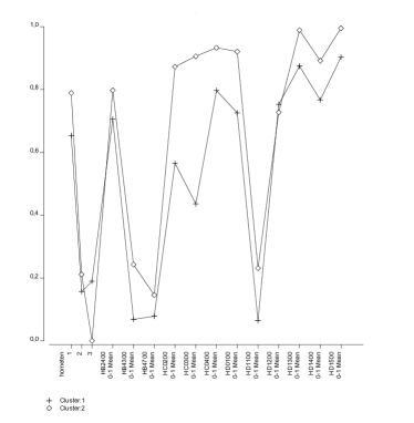
(a) LCreg, $S=2$

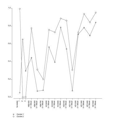
(b) LCcw, $S=2$

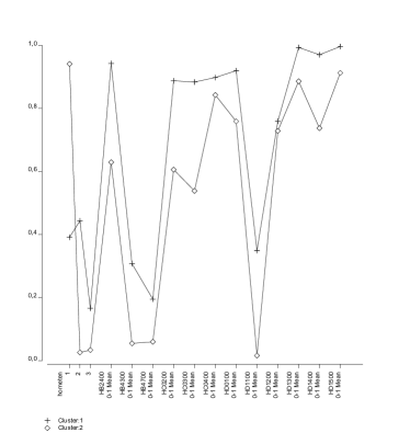
(c) LCdist, $S=2$

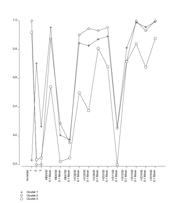
(d) LCdist, $S=3$

Figure 4: Probability profile plot for LCreg $(S=2)$, LCdist $(S=2$ and $S=3$) and LCcw $(S=2)$. For the variable “hometen”, the levels indicate the four category ownership probabilities within each wealth class. Similarly, levels refer to average item ownership probability in wealth classes for the remaining (dichotomous) items.

We observe that both the LCreg and the LCcw models, contrary to the two-class LCdist model, predict a wealthier class, with higher ownership probabilities for all items, and a higher probability of owning (partially or entirely) the household main residence - relative to “free use” and “rent” categories. In the three-class LCdist model, whose first and second clusters seem to arise from a split of the first cluster of the two-class model, the first wealth class shows higher ownership probabilities for all items, and a higher probability of owning (partially or entirely) the household main residence, as in the two-class LCreg and LCcw models. One possible explanation for this is that the LCdist model needs one additional class to predict a class profile reasonably corresponding to the highest wealth level. Interestingly, profiles of all three models ($S=2$) are comparable, though each showing specific features. LCreg classes have a similar composition in terms of profiles. Both LCdist ($S=2$ and $S=3$) and LCcw deliver better separated classes. However, wealthier households are predicted by LCcw to own more assets, whereas less wealthy household have a relatively larger probability, for instance, to have a rented (or for free use) residence.

Table 13 reports the ARI for pairwise comparisons of the three models. LCdist, with both $S=2$ and $S=3$, and LCcw deliver clusterings with moderate agreement. Figure 5d shows how the class composition of LCdist (with $S=2$ and $S=3$) and LCcw predicts classes in log-wealth.

	LCreg	LCdist	LCdist	LCcwm
		$(S=2)$	$(S=3)$
LCreg	1
LCdist $(S=2)$	0.0869	1
LCdist $(S=3)$	0.3369	0.4446	1
LCcw	0.0661	0.4676	0.4371	1

Table 13: Adjusted Rand indexes comparing clustering in classes of wealth of LCreg, LCdist and LCcw models.

The first class in LCdist with $S=2$ (Figure 5a) seems to capture observations with lower log-wealth, although its relatively fat tails allocate non-zero density also to the wealthiest observations. With $S=3$ (Figure 5b), the second class is split into two (see also Figure 5d), with the new third class made up of households in the right tale of log-wealth distribution. Consistently with findings in the probability profiles, classes in LCcw are able to discriminate households better in terms of prediction of the (log) wealth distribution (Figure 5c).

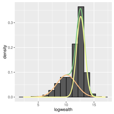
(a) LCdist, $S=2$

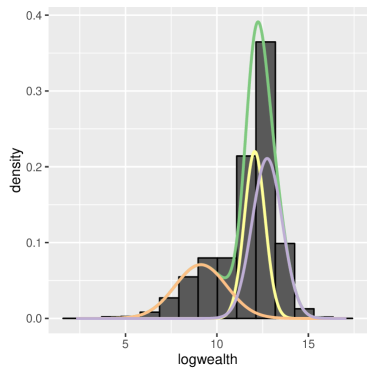
(b) LCdist, $S=3$

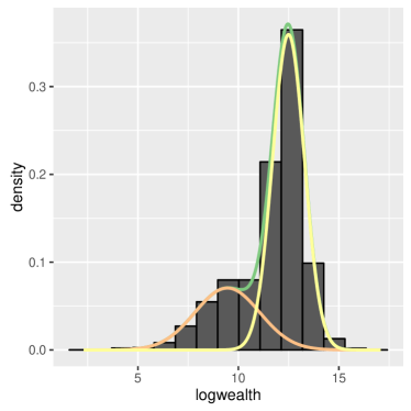
(c) LCcw

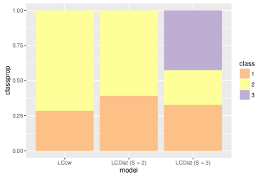
(d) Class proportions

Figure 5: Density plots of log-wealth as predicted by LCdist $(S=2$, a, and $S=3$,b) and LCcw (c). Mixture density in green, component marginal densities in other colors. Class proportions in (d).

To gain further insights on the estimated wealth distribution, we report (Table 14) estimated means and variances of log-wealth, for LCdist with $S=2$ and LCcw. For comparability, we choose not to report mean and variance values for LCdist with $S=3$.

	Means		Wald(=) $p$	Variances		Wald(=) $p$
LCdist	10.0835***	12.6173***	0.0000	3.0910	0.5573	0.0000
	(0.0451)	(0.0129)		(0.0843)	(0.0137)
LCcw	9.4489***	12.4928***	0.0000	2.5960	0.6304	0.0380
	(0.0391)	(0.0112)		(0.0865)	(0.0131)

Table 14: Estimated means (*** $p$-value$<$0.01, ** $p$-value$<$0.05, * $p$-value$<$0.1) and variances of log-wealth, and $p$-values from Wald test of equality of component means and variances for the LCdist $(S=2)$ and LCcw models. Standard errors in parentheses.

Inference on the estimated parameters of the log-wealth ($p$-values of all tests are below 0.01) validates the model assumption of clustered distribution, with heteroscedastic components, of log-wealth in both LCdist and LCcw. The mean in the first class of wealth is larger for LCdist than for LCcw, along with the related variance. As we observed above, this first class in LCdist absorbs also households in the right tale of the distribution. This complicates the interpretation of the wealth classes compared to LCcw. That is, LCcw, with a first class with smaller mean and variance, allows for a more natural substantive interpretation of the two classes as wealthier versus less wealthy households. This is also consistent with findings of the related literature on poverty (deprivation) (Moisio, 2004; Pérez-Mayo, 2005).

Finally, Table 15 demonstrates that LCcw provides an easy way to test whether there are significant direct effects of log-wealth on the response variables. Interestingly, inference on such effects points out that there are variables for which we have no significant direct effects of log-wealth (hometen), as well as indicating that some effects are the same across latent classes (HB2400, HD1300, HD1400 and HD1500). In the logic of an applied researcher, this suggests intermediate and more parsimonious modeling options, where effects on some variables can be constrained to be zero, or to be the same across classes, which can easily be discovered with a cluster-weighted modeling approach.

Log-wealth on	Coefficients		Wald(0) $p$	Wald(=) $p$
	Class 1	Class 2
hometen	0.0184	0.1532	0.6800	0.4800
(Main res. tenure stat)	(0.0392)	(0.1930)
HB2400	-1.6242***	-1.5421***	0.0000	0.4600
(HH owns other properties)	(0.0957)	(0.0564)
HB4300	-0.5784***	-1.1729***	0.0000	0.0000
(HH owns any car)	(0.0426)	(0.0626)
HB4700	-0.3866***	-0.7445***	0.0000	0.0000
(HH owns other valuables)	(0.0396)	(0.0639)
HC0200	-0.5217***	-0.7899***	0.0000	0.0000
(HH has a credit line)	(0.0431)	(0.0433)
HC0300	-0.8741***	-1.1398***	0.0000	0.0001
(HH has a credit card)	(0.0517)	(0.0480)
HC0400	-0.2026***	-0.2205***	0.0000	0.7800
(HH has a non-coll. loan)	(0.0415)	(0.0515)
HD0100	-0.7896***	-1.0633***	0.0000	0.0002
(HH has any invest. in business)	(0.0536)	(0.0527)
HD1100	-0.8060***	-1.6133***	0.0000	0.0000
(HH owns a sight account)	(0.0463)	(0.0768)
HD1200	-0.2216***	-0.0630*	0.0000	0.0025
(HH owns a savings account)	(0.0364)	(0.0381)
HD1300	-1.0827***	-1.1224***	0.0000	0.7500
(HH has invest. in mutual funds)	(0.1061)	(0.0636)
HD1400	-0.9244***	-0.9835***	0.0000	0.5100
(HH owns bonds)	(0.0766)	(0.0478)
HD1500	-1.0942***	-1.1664***	0.0000	0.6100
(HH owns managed accounts)	(0.1236)	(0.0688)

Table 15: Estimated direct effects of log-wealth on each variable per latent class (*** $p$-value$<$0.01, ** $p$-value$<$0.05, * $p$-value$<$0.1), $p$-values from Wald test of joint equality of each variable’s direct effect to zero - Wald(0) - and from Wald test of equality of effects across latent classes - Wald(=) - for the LCcw model. Short description below variable names. HH stands for Household. Standard errors in parentheses.

5 Conclusion

In this paper we have brought modeling ideas from the regression mixture literature into latent class analysis. Our focus has been to motivate the use of the cluster-weighted modeling approach as a general specification for the joint relationship of the response variables, the external variable, and the latent variable. Three population studies have been used to illustrate this idea, and the actual advantage of the proposed approach was showed through an application on Italian household asset ownership data.

The cluster-weighted modeling approach, contrary to the simpler distal outcome model, was able to predict, based on the joint relationship of ownership indicators, the underlying true wealth, and wealth as measured by the survey, two interpretable classes of wealth with class ownership profiles coinciding respectively with less wealthy (first class) and wealthier (second class) households on the measured log-wealth distribution.

In the applied researcher perspective, the proposed approach has several advantages. First, it allows to deal with direct effects if this are of substantive interest, as well as if those represent a source of noise to be handled. That is, if direct effects are present, our approach, contrary to the distal outcome model, yields unbiased estimates of the distal outcome cluster specific means and variances. Second, it guarantees a safe and flexible option, in which one starts from the most general model. Then, proceeding backwards, the user can test the model assumptions of both the distal outcome and the latent class regression models.

The approach we suggest has some limitations as well. First, it can be unstable if some of the observed response patterns are lacking, or are simply too small in number to estimate the model parameters (see for instance, for standard sufficient conditions for identifiability of LCA, Bandeen-Roche ., 1997). Especially in an exploratory stage of the analysis, in such cases simpler models can be more attractive. Second, depending on the goal of the analysis, the cluster-weighted modeling approach can generate a final output which might be harder to interpret than that of simpler models. In other words, the final model interpretability relies on the final goal of the analysis, which must be clear in mind in this as well as in any other modeling approach.

Appendix A Latent GOLD syntax for the three models

A.1 LCreg model syntax

options

maxthreads=4;

algorithm

tolerance=1e-008 emtolerance=0.01 emiterations=500 nriterations=100 ;

startvalues

seed=0 sets=50 tolerance=1e-005 iterations=50;

bayes

categorical=1 variances=1 latent=1 poisson=1;

montecarlo

seed=0 sets=0 replicates=500 tolerance=1e-008;

quadrature nodes=10;

missing excludeall;

output

parameters=first betaopts=wl standarderrors profile probmeans=posterior

bivariateresiduals estimatedvalues=model;

variables

dependent hometen nominal, HB2400, HB4300, HB4700, HC0200,

HC0300, HC0400, HD0100,

HD1100, HD1200, HD1300, HD1400, HD1500;

independent logwealth;

latent

Cluster nominal 2;

equations

Cluster $<-$ 1;

hometen $<-$ 1$|$Cluster + logwealth$|$Cluster;

HB2400 $<-$ 1$|$Cluster + logwealth$|$Cluster;

HB4300 $<-$ 1$|$Cluster + logwealth$|$Cluster;

HB4700 $<-$ 1$|$Cluster + logwealth$|$Cluster;

HC0200 $<-$ 1$|$Cluster + logwealth$|$Cluster;

HC0300 $<-$ 1$|$Cluster + logwealth$|$Cluster;

HC0400 $<-$ 1$|$Cluster + logwealth$|$Cluster;

HD0100 $<-$ 1$|$Cluster + logwealth$|$Cluster;

HD1100 $<-$ 1$|$Cluster + logwealth$|$Cluster;

HD1200 $<-$ 1$|$Cluster + logwealth$|$Cluster;

HD1300 $<-$ 1$|$Cluster + logwealth$|$Cluster;

HD1400 $<-$ 1$|$Cluster + logwealth$|$Cluster;

HD1500 $<-$ 1$|$Cluster + logwealth$|$Cluster;

A.2 LCdist model syntax

options

maxthreads=4;

algorithm

tolerance=1e-008 emtolerance=0.01 emiterations=500 nriterations=50 ;

startvalues

seed=0 sets=50 tolerance=1e-005 iterations=50;

bayes

categorical=1 variances=1 latent=1 poisson=1;

montecarlo

seed=0 sets=0 replicates=500 tolerance=1e-008;

quadrature nodes=10;

missing excludeall;

output

parameters=first betaopts=wl standarderrors profile probmeans=posterior

bivariateresiduals estimatedvalues=model;

variables

dependent hometen nominal, HB2400, HB4300, HB4700, HC0200,

HC0300, HC0400, HD0100,

HD1100, HD1200, HD1300, HD1400, HD1500, logwealth continuous;

latent

Cluster nominal 2;

equations

Cluster $<-$ 1;

hometen $<-$ 1$|$Cluster;

HB2400 $<-$ 1$|$Cluster;

HB4300 $<-$ 1$|$Cluster;

HB4700 $<-$ 1$|$Cluster;

HC0200 $<-$ 1$|$Cluster;

HC0300 $<-$ 1$|$Cluster;

HC0400 $<-$ 1$|$Cluster;

HD0100 $<-$ 1$|$Cluster;

HD1100 $<-$ 1$|$Cluster;

HD1200 $<-$ 1$|$Cluster;

HD1300 $<-$ 1$|$Cluster;

HD1400 $<-$ 1$|$Cluster;

HD1500 $<-$ 1$|$Cluster;

logwealth $<-$ 1$|$Cluster;

logwealth$|$Cluster;

A.3 LCCw model syntax

Notice that “logwealthshadow” is a duplicate of “logwealth”, as Latent GOLD does not allow the same variable to be both dependent and independent variable at the same time.

options

maxthreads=4;

algorithm

tolerance=1e-008 emtolerance=0.01 emiterations=500 nriterations=50 ;

startvalues

seed=0 sets=50 tolerance=1e-005 iterations=50;

bayes

categorical=1 variances=1 latent=1 poisson=1;

montecarlo

seed=0 sets=0 replicates=500 tolerance=1e-008;

quadrature nodes=10;

missing excludeall;

output

parameters=first betaopts=wl standarderrors profile probmeans=posterior

bivariateresiduals estimatedvalues=model;

variables

dependent hometen nominal, HB2400, HB4300, HB4700, HC0200,

HC0300, HC0400, HD0100,

HD1100, HD1200, HD1300, HD1400, HD1500, logwealth continuous;

independent logwealthshadow;

latent

Cluster nominal 2;

equations

Cluster $<-$ 1; hometen $<-$ 1$|$Cluster + logwealthshadow$|$Cluster;

HB2400 $<-$ 1$|$Cluster + logwealthshadow$|$Cluster;

HB4300 $<-$ 1$|$Cluster + logwealthshadow$|$Cluster;

HB4700 $<-$ 1$|$Cluster + logwealthshadow$|$Cluster;

HC0200 $<-$ 1$|$Cluster + logwealthshadow$|$Cluster;

HC0300 $<-$ 1$|$Cluster + logwealthshadow$|$Cluster;

HC0400 $<-$ 1$|$Cluster + logwealthshadow$|$Cluster;

HD0100 $<-$ 1$|$Cluster + logwealthshadow$|$Cluster;

HD1100 $<-$ 1$|$Cluster + logwealthshadow$|$Cluster;

HD1200 $<-$ 1$|$Cluster + logwealthshadow$|$Cluster;

HD1300 $<-$ 1$|$Cluster + logwealthshadow$|$Cluster;

HD1400 $<-$ 1$|$Cluster + logwealthshadow$|$Cluster;

HD1500 $<-$ 1$|$Cluster + logwealthshadow$|$Cluster;

logwealth $<-$ 1$|$Cluster;

logwealth$|$Cluster;

References

- Asparouhov \BBA Muthén (\APACyear2014) \APACinsertmetastarasparouhov2012auxiliary{APACrefauthors}Asparouhov, T.\BCBT \BBA Muthén, B. \APACrefYearMonthDay2014. \BBOQ\APACrefatitleAuxiliary variables in mixture modeling: Three-step approaches using Mplus Auxiliary variables in mixture modeling: Three-step approaches using Mplus.\BBCQ \APACjournalVolNumPagesStructural Equation Modeling21329-341. \PrintBackRefs\CurrentBib
- Bakk \BOthers. (\APACyear2013) \APACinsertmetastarbakk:12{APACrefauthors}Bakk, Z., Tekle, F\BPBIT.\BCBL \BBA Vermunt, J\BPBIK. \APACrefYearMonthDay2013. \BBOQ\APACrefatitleEstimating the association between latent class membership and external variables using bias-adjusted three-step approaches Estimating the association between latent class membership and external variables using bias-adjusted three-step approaches.\BBCQ \APACjournalVolNumPagesSociological Methodology272-311. \PrintBackRefs\CurrentBib
- Bandeen-Roche \BOthers. (\APACyear1997) \APACinsertmetastarbandeenroche:97{APACrefauthors}Bandeen-Roche, K., Miglioretti, D.\BCBL \BBA Zegger, P., S.L. Rathouz. \APACrefYearMonthDay1997. \BBOQ\APACrefatitleLatent variable regression for multiple discrete outcomes Latent variable regression for multiple discrete outcomes.\BBCQ \APACjournalVolNumPagesJournal of the American Statistical Association921375-86. \PrintBackRefs\CurrentBib
- Bouwmeester \BBA Sijtsma (\APACyear2007) \APACinsertmetastarbouwmeester{APACrefauthors}Bouwmeester, S.\BCBT \BBA Sijtsma, K. \APACrefYearMonthDay2007. \BBOQ\APACrefatitleLatent Class Modeling of Phases in the Development of Transitive Reasoning Latent class modeling of phases in the development of transitive reasoning.\BBCQ \APACjournalVolNumPagesMultivariate Behavioral Research423457–480. \PrintBackRefs\CurrentBib
- Charles \BBA Hurst (\APACyear2003) \APACinsertmetastarcharles2003{APACrefauthors}Charles, K\BPBIK.\BCBT \BBA Hurst, E. \APACrefYearMonthDay2003. \BBOQ\APACrefatitleThe correlation of wealth across generations The correlation of wealth across generations.\BBCQ \APACjournalVolNumPagesJournal of Political Economy11161155–1182. \PrintBackRefs\CurrentBib
- Collins \BBA Lanza (\APACyear2010) \APACinsertmetastarcollins2010latent{APACrefauthors}Collins, L\BPBIM.\BCBT \BBA Lanza, S\BPBIT. \APACrefYear2010. \APACrefbtitleLatent class and latent transition analysis: With applications in the social, behavioral, and health sciences Latent class and latent transition analysis: With applications in the social, behavioral, and health sciences (\BVOL 718). \APACaddressPublisherWiley. \PrintBackRefs\CurrentBib
- Dang \BOthers. (\APACyear2017) \APACinsertmetastarDang:Punz:McNi:Ingr:Brow:Mult:2017{APACrefauthors}Dang, U\BPBIJ., Punzo, A., McNicholas, P\BPBID., Ingrassia, S.\BCBL \BBA Browne, R\BPBIP. \APACrefYearMonthDay2017. \BBOQ\APACrefatitleMultivariate Response and Parsimony for Gaussian Cluster-Weighted Models Multivariate response and parsimony for Gaussian cluster-weighted models.\BBCQ \APACjournalVolNumPagesJournal of Classification3414–34. \PrintBackRefs\CurrentBib
- Dayton \BBA Macready (\APACyear1988) \APACinsertmetastardayton{APACrefauthors}Dayton, C\BPBIM.\BCBT \BBA Macready, G\BPBIB. \APACrefYearMonthDay1988. \BBOQ\APACrefatitleConcomitant-variable latent class models. Concomitant-variable latent class models.\BBCQ \APACjournalVolNumPagesJournal of the American Statistical Association83173-178. \PrintBackRefs\CurrentBib
- Di Mari \BBA Bakk (\APACyear2017) \APACinsertmetastarrobzsuzsa17{APACrefauthors}Di Mari, R.\BCBT \BBA Bakk, Z. \APACrefYearMonthDay2017. \BBOQ\APACrefatitleMostly harmless direct effects: a comparison of different latent Markov modeling approaches Mostly harmless direct effects: a comparison of different latent markov modeling approaches.\BBCQ \APACjournalVolNumPagesStructural Equation Modeling: A Multidisciplinary Journal. \PrintBackRefs\CurrentBib
- Ferguson \BOthers. (\APACyear2003) \APACinsertmetastarferguson2003{APACrefauthors}Ferguson, B\BPBID., Tandon, A., Gakidou, E.\BCBL \BBA Murray, C\BPBIJ. \APACrefYearMonthDay2003. \BBOQ\APACrefatitleEstimating permanent income using indicator variables Estimating permanent income using indicator variables.\BBCQ \APACjournalVolNumPagesHealth systems performance assessment: debates, methods and empiricism. Geneva: World Health Organization747–760. \PrintBackRefs\CurrentBib
- Friedman (\APACyear1957) \APACinsertmetastarfriedman1957{APACrefauthors}Friedman, M. \APACrefYear1957. \APACrefbtitleA Theory of the Consumption Function A theory of the consumption function. \APACaddressPublisherPrinceton: Princeton University Press. \PrintBackRefs\CurrentBib
- Hagenaars \BBA Halman (\APACyear1989) \APACinsertmetastarhagenaars1989{APACrefauthors}Hagenaars, J\BPBIA.\BCBT \BBA Halman, L\BPBIC. \APACrefYearMonthDay1989. \BBOQ\APACrefatitleSearching for idealtypes: the potentialities of latent class analysis Searching for idealtypes: the potentialities of latent class analysis.\BBCQ \APACjournalVolNumPagesEuropean Sociological Review5181–96. \PrintBackRefs\CurrentBib
- Household Finance and Consumption Network (\APACyear2013) \APACinsertmetastarecb2013{APACrefauthors}Household Finance and Consumption Network. \APACrefYearMonthDay2013. \APACrefbtitleThe Eurosystem Household Finance and Consumption Survey-Methodological report The eurosystem household finance and consumption survey-methodological report \APACbVolEdTR\BTR. \APACaddressInstitutionECB Statistics Paper. \PrintBackRefs\CurrentBib
- Hubert \BBA Arabie (\APACyear1985) \APACinsertmetastarhubertARI{APACrefauthors}Hubert, L.\BCBT \BBA Arabie, P. \APACrefYearMonthDay1985. \BBOQ\APACrefatitleComparing partitions Comparing partitions.\BBCQ \APACjournalVolNumPagesJournal of Classification21193–218. \PrintBackRefs\CurrentBib
- Ingrassia \BOthers. (\APACyear2012) \APACinsertmetastaringrassia2012{APACrefauthors}Ingrassia, S., Minotti, S.\BCBL \BBA Vittadini, G. \APACrefYearMonthDay2012. \BBOQ\APACrefatitleLocal statistical modeling via a cluster–weighted approach with elliptical distributions Local statistical modeling via a cluster–weighted approach with elliptical distributions.\BBCQ \APACjournalVolNumPagesJournal of Classification29363–401. \PrintBackRefs\CurrentBib
- Ingrassia \BOthers. (\APACyear2014) \APACinsertmetastarIngr:Mino:Punz:Mode:2014{APACrefauthors}Ingrassia, S., Minotti, S\BPBIC.\BCBL \BBA Punzo, A. \APACrefYearMonthDay2014. \BBOQ\APACrefatitleModel-based clustering via linear cluster-weighted models Model-based clustering via linear cluster-weighted models.\BBCQ \APACjournalVolNumPagesComputational Statistics & Data Analysis71159–182. \PrintBackRefs\CurrentBib
- Ingrassia \BOthers. (\APACyear2015) \APACinsertmetastarIngr:Punz:Vitt:TheG:2015{APACrefauthors}Ingrassia, S., Punzo, A., Vittadini, G.\BCBL \BBA Minotti, S\BPBIC. \APACrefYearMonthDay2015. \BBOQ\APACrefatitleThe Generalized Linear Mixed Cluster-Weighted Model The generalized linear mixed cluster-weighted model.\BBCQ \APACjournalVolNumPagesJournal of Classification32185–113. \PrintBackRefs\CurrentBib
- Kamakura \BBA Russel (\APACyear1989) \APACinsertmetastarkamakura1989{APACrefauthors}Kamakura, W\BPBIA.\BCBT \BBA Russel, G. \APACrefYearMonthDay1989. \BBOQ\APACrefatitleA Probabilistic Choice Model for Market Segmentation and Elasticity Structure A probabilistic choice model for market segmentation and elasticity structure.\BBCQ \APACjournalVolNumPagesJournal of Marketing Research264379–390. \PrintBackRefs\CurrentBib
- Kim \BOthers. (\APACyear2016) \APACinsertmetastarleepaper{APACrefauthors}Kim, M., Vermunt, J\BPBIK., Bakk, Z., Jaki, T.\BCBL \BBA Van Horn, M\BPBIL. \APACrefYearMonthDay2016. \BBOQ\APACrefatitleModeling Predictors of Latent Classes in Regression Mixture Models Modeling predictors of latent classes in regression mixture models.\BBCQ \APACjournalVolNumPagesStructural Equation Modeling: A Multidisciplinary Journal23601-614. \PrintBackRefs\CurrentBib
- Lanza \BOthers. (\APACyear2013) \APACinsertmetastarlanza:13{APACrefauthors}Lanza, T\BPBIS., Tan, X.\BCBL \BBA Bray, C\BPBIB. \APACrefYearMonthDay2013. \BBOQ\APACrefatitleLatent Class Analysis With Distal Outcomes: A Flexible Model-Based Approach Latent class analysis with distal outcomes: A flexible model-based approach.\BBCQ \APACjournalVolNumPagesStructural Equation Modeling2011-26. \PrintBackRefs\CurrentBib
- Loken (\APACyear2004) \APACinsertmetastarloken2004{APACrefauthors}Loken, E. \APACrefYearMonthDay2004. \BBOQ\APACrefatitleUsing Latent Class Analysis to Model Temperament Types Using latent class analysis to model temperament types.\BBCQ \APACjournalVolNumPagesMultivariate Behavioral Research394625–652. \PrintBackRefs\CurrentBib
- Magidson (\APACyear1981) \APACinsertmetastarmagidson81{APACrefauthors}Magidson, J. \APACrefYearMonthDay1981. \BBOQ\APACrefatitleQualitative variance, entropy, and correlation ratios for nominal dependent variables Qualitative variance, entropy, and correlation ratios for nominal dependent variables.\BBCQ \APACjournalVolNumPagesSocial Science Research10. \PrintBackRefs\CurrentBib
- Maij-de Meij \BOthers. (\APACyear2005) \APACinsertmetastarhenk{APACrefauthors}Maij-de Meij, A\BPBIM., Kelderman, H.\BCBL \BBA van der Flier, H. \APACrefYearMonthDay2005. \BBOQ\APACrefatitleLatent-trait latent-class analysis of self-disclosure in the work environment Latent-trait latent-class analysis of self-disclosure in the work environment.\BBCQ \APACjournalVolNumPagesMultivariate Behavioral Research404435–459. \PrintBackRefs\CurrentBib
- McCutcheon (\APACyear1985) \APACinsertmetastarmccutcheon1985latent{APACrefauthors}McCutcheon, A\BPBIL. \APACrefYearMonthDay1985. \BBOQ\APACrefatitleA latent class analysis of tolerance for nonconformity in the American public A latent class analysis of tolerance for nonconformity in the american public.\BBCQ \APACjournalVolNumPagesPublic Opinion Quarterly494474–488. \PrintBackRefs\CurrentBib
- Moisio (\APACyear2004) \APACinsertmetastarmoisio2004{APACrefauthors}Moisio, P. \APACrefYearMonthDay2004. \BBOQ\APACrefatitleA latent class application to the multidimensional measurement of poverty A latent class application to the multidimensional measurement of poverty.\BBCQ \APACjournalVolNumPagesQuality & Quantity386703–717. \PrintBackRefs\CurrentBib
- Moore \BBA Welniak (\APACyear2000) \APACinsertmetastarmoore2000{APACrefauthors}Moore, J\BPBIC.\BCBT \BBA Welniak, E\BPBIJ. \APACrefYearMonthDay2000. \BBOQ\APACrefatitleIncome measurement error in surveys: A review Income measurement error in surveys: A review.\BBCQ \APACjournalVolNumPagesJournal of Official Statistics164331. \PrintBackRefs\CurrentBib
- Mulder \BOthers. (\APACyear2012) \APACinsertmetastarmulder2012{APACrefauthors}Mulder, E., Vermunt, J., Brand, E., Bullens, R.\BCBL \BBA Van Merle, H. \APACrefYearMonthDay2012. \BBOQ\APACrefatitleRecidivism in subgroups of serious juvenile offenders: Different profiles, different risks? Recidivism in subgroups of serious juvenile offenders: Different profiles, different risks?\BBCQ \APACjournalVolNumPagesCriminal Behaviour and Mental Health22122–135. \PrintBackRefs\CurrentBib
- Nylund-Gibson \BBA Masyn (\APACyear2016) \APACinsertmetastarnylund16{APACrefauthors}Nylund-Gibson, K.\BCBT \BBA Masyn, K\BPBIE. \APACrefYearMonthDay2016. \BBOQ\APACrefatitleCovariates and Mixture Modeling: Results of a Simulation Study Exploring the Impact of Misspecified Effects on Class Enumeration Covariates and mixture modeling: Results of a simulation study exploring the impact of misspecified effects on class enumeration.\BBCQ \APACjournalVolNumPagesStructural Equation Modeling: A Multidisciplinary Journal23782-797. \PrintBackRefs\CurrentBib
- Okazaki \BOthers. (\APACyear2015) \APACinsertmetastarokazaki15{APACrefauthors}Okazaki, S., Campo, S., Andreu, L.\BCBL \BBA Romero, J. \APACrefYearMonthDay2015. \BBOQ\APACrefatitleA latent class analysis of Spanish travelers’ mobile internet usage in travel planning and execution A latent class analysis of spanish travelers’ mobile internet usage in travel planning and execution.\BBCQ \APACjournalVolNumPagesCornell Hospitality Quarterly562191–201. \PrintBackRefs\CurrentBib
- Pérez-Mayo (\APACyear2005) \APACinsertmetastarperez2005{APACrefauthors}Pérez-Mayo, J. \APACrefYearMonthDay2005. \BBOQ\APACrefatitleIdentifying deprivation profiles in Spain: a new approach Identifying deprivation profiles in spain: a new approach.\BBCQ \APACjournalVolNumPagesApplied Economics378943–955. \PrintBackRefs\CurrentBib
- Punzo (\APACyear2014) \APACinsertmetastarPunz:Flex:2014{APACrefauthors}Punzo, A. \APACrefYearMonthDay2014. \BBOQ\APACrefatitleFlexible Mixture Modeling with the Polynomial Gaussian Cluster-Weighted Model Flexible mixture modeling with the polynomial Gaussian cluster-weighted model.\BBCQ \APACjournalVolNumPagesStatistical Modelling143257–291. \PrintBackRefs\CurrentBib
- R Core Team (\APACyear2017) \APACinsertmetastarrcore{APACrefauthors}R Core Team. \APACrefYearMonthDay2017. \BBOQ\APACrefatitleR: A Language and Environment for Statistical Computing R: A language and environment for statistical computing\BBCQ [\bibcomputersoftwaremanual]. \APACaddressPublisherVienna, Austria. {APACrefURL} https://www.R-project.org/ \PrintBackRefs\CurrentBib
- Roberts \BBA Ward (\APACyear2011) \APACinsertmetastarroberts2011{APACrefauthors}Roberts, T\BPBIJ.\BCBT \BBA Ward, S\BPBIE. \APACrefYearMonthDay2011. \BBOQ\APACrefatitleUsing latent transition analysis in nursing research to explore change over time Using latent transition analysis in nursing research to explore change over time.\BBCQ \APACjournalVolNumPagesNursing research60173–79. \PrintBackRefs\CurrentBib
- Roedelof \BOthers. (\APACyear2013) \APACinsertmetastarroedelof13{APACrefauthors}Roedelof, A\BPBIJ\BPBIM., Bongers, I\BPBIL.\BCBL \BBA van Nieuwenhuizen, C. \APACrefYearMonthDay2013. \BBOQ\APACrefatitleTreatment engagement in adolescents with severe psychiatric problems: a latent class analysis Treatment engagement in adolescents with severe psychiatric problems: a latent class analysis.\BBCQ \APACjournalVolNumPagesEuropean Child and Adolescent Psychiatry228491–500. \PrintBackRefs\CurrentBib
- Stegmann \BBA Grimm (\APACyear2017) \APACinsertmetastarstegmann2017{APACrefauthors}Stegmann, G.\BCBT \BBA Grimm, K\BPBIJ. \APACrefYearMonthDay2017. \BBOQ\APACrefatitleA New Perspective on the Effects of Covariates in Mixture Models A new perspective on the effects of covariates in mixture models.\BBCQ \APACjournalVolNumPagesStructural Equation Modeling: A Multidisciplinary Journal. \PrintBackRefs\CurrentBib
- Szeles \BBA Fusco (\APACyear2013) \APACinsertmetastarszeles2013{APACrefauthors}Szeles, M\BPBIR.\BCBT \BBA Fusco, A. \APACrefYearMonthDay2013. \BBOQ\APACrefatitleItem response theory and the measurement of deprivation: evidence from Luxembourg data Item response theory and the measurement of deprivation: evidence from luxembourg data.\BBCQ \APACjournalVolNumPagesQuality & Quantity1–16. \PrintBackRefs\CurrentBib
- Vandemoortele (\APACyear2014) \APACinsertmetastarvandemoortele2014{APACrefauthors}Vandemoortele, M. \APACrefYearMonthDay2014. \BBOQ\APACrefatitleMeasuring household wealth with latent trait modelling: an application to Malawian DHS Data Measuring household wealth with latent trait modelling: an application to malawian dhs data.\BBCQ \APACjournalVolNumPagesSocial Indicators Research1182877–891. \PrintBackRefs\CurrentBib
- Vermunt (\APACyear2010) \APACinsertmetastarvermunt:10{APACrefauthors}Vermunt, J\BPBIK. \APACrefYearMonthDay2010. \BBOQ\APACrefatitleLatent Class Modeling with Covariates: Two Improved Three-Step Approaches Latent class modeling with covariates: Two improved three-step approaches.\BBCQ \APACjournalVolNumPagesPolitical Analysis18450-469. \PrintBackRefs\CurrentBib
- Vermunt \BBA Magidson (\APACyear2016) \APACinsertmetastarlatentG5.1{APACrefauthors}Vermunt, J\BPBIK.\BCBT \BBA Magidson, J. \APACrefYearMonthDay2016. \BBOQ\APACrefatitleTechnical guide for Latent GOLD 5.1: Basic, advanced, and syntax Technical guide for latent gold 5.1: Basic, advanced, and syntax.\BBCQ \APACjournalVolNumPagesBelmont, MA: Statistical Innovations Inc.. \PrintBackRefs\CurrentBib
- Wedel \BBA DeSarbo (\APACyear1994) \APACinsertmetastarwedel94{APACrefauthors}Wedel, M.\BCBT \BBA DeSarbo, W. \APACrefYearMonthDay1994. \BBOQ\APACrefatitleA review of recent developments in latent class regression models A review of recent developments in latent class regression models.\BBCQ \BIn R. Bagozzi (\BED), \APACrefbtitleAdvanced Methods of Marketing Research Advanced methods of marketing research (\BPGS 352–388). \APACaddressPublisherCambridge, Massachusetts: Blackwell Publishers. \PrintBackRefs\CurrentBib