A Phase Transition in a Widom-Rowlinson Model with Curie-Weiss Interaction

Abstract.

An analog of the continuum Widom-Rowlinson model is introduced and studied. Its two-component version is a gas of point particles of types 0 and 1 placed in $\mathds{R}^{d}$, in which like particles do not interact and unlike particles contained in a vessel of volume $V$ repel each other with intensity $a/V$. The one-component version is a gas of particles with multi-particle interactions of Curie-Weiss type. Its thermodynamic behavior is obtained by integrating out the coordinates of one of the components of the two-component version. In the grand canonical setting, a rigorous theory of phase transitions in this model is developed and discussed. In particular, for both versions thermodynamic phases and phase diagrams are explicitly constructed and the equations of state are obtained and analyzed.

1. Introduction

The rigorous theory of thermal equilibrium of continuum particle systems has got much more modest results than its counterpart dealing with lattices, graphs, etc. There exist only few ‘realistic’ models in which the existence of a liquid-vapor phase transition was mathematically proved. Among them there is the model introduced in [1] by B. Widom and J. S. Rowlinson in which the potential energy of $n$ point particles located at $x_{1},\dots,x_{n}\in\mathds{R}^{d}$ is set to be $\theta[W(x_{1},\dots,x_{n})-n]$, where $\theta>0$ is a parameter and $W$ is the volume of the area $\cup_{i=1}^{n}B(x_{i})$ covered by the balls of unite volume centered at these particles. The thermodynamics of this model is in a sense equivalent to that of a two-component system with binary interactions in which the interaction between unlike particles is a hard-core repulsion and is zero otherwise. In [2], D. Ruelle proved that the two-component system in two or more dimensions undergoes a phase transition of first order. Later on, the rigorous theory of this model was extended in [3], see also [4] for a review. However, these results give a little for understanding the details of the phenomenon. No rigorous results are available on the behavior at the phase-transition threshold. The very existence of such a threshold remains unknown. At the same time, for a number of lattice models the mean field approach allows for understanding phase transitions in the corresponding models with ‘realistic’ interactions, see [5]. It is then quite natural to develop the mean field theory of phase transitions also in continuum systems. For the Widom-Rowlinson model, the first attempt to do this was undertaken already in [1, Sect. VII]. Assuming that the particles are distributed in a given vessel “at random” the authors heuristically deduced an equation of state [1, eq. (7.4)], which manifests a first order phase transition. One of the ways to develop a mean field theory in a rigorous way is to use Curie-Weiss interaction potentials, see [6] and [7, Sect. IV.4]. The aim of this work is to perform a rigorous study of this kind of an analog of the Widom-Rowlinson model with Curie-Weiss interactions, which we introduce in Section 2 below. Similarly to the original Widom-Rowlinson model, it has two versions: (a) a two-component gas of point particles with binary repulsion of unlike particles; (b) a one-component gas with multi-particle interactions the states of which are obtained by ‘integrating out’ the coordinates of one of the components of the two-component system. The phase diagrams and the thermodynamic phases of these versions are described in Theorems 2.2 and 2.3, respectively. Unlike to [6, 8] we work in the grand canonical ensemble approach and – along with a traditional purely thermodynamic description – we explicitly construct thermodynamic phases and show their multiplicity occurring for certain values of the particle activities. The formulation of the results is followed by their detailed discussion in the same Section 2. The validity of Theorem 2.3 directly follows from Theorem 2.2. The proof of Theorem 2.2 is performed in Section 3. As is usual for Curie-Weiss interactions, the thermodynamic limit is achieved by calculating asymptotics of certain integrals, cf [7, Theorem IV.4.1]. Unlike to lattice system where this is mostly done by directly applying Laplace’s method, here we have to overcome technical difficulties related to a more complex dependence of the integrands on the ‘large parameter’.

2. The Setup

In this work, $\mathds{N}$ and $\mathds{R}$ will stand for the sets of natural and real numbers, respectively; also $\mathds{N}_{0}:=\mathds{N}\cup\{0\}$. For $d\in\mathds{N}$, by $\mathds{R}^{d}$ we denote the Euclidean space of vectors $x=(x^{1},\dots,x^{d})$, $x^{i}\in\mathds{R}$, equipped with the usual Lebesgue measure $dx$.

2.1. The model

States of thermal equilibrium of infinite systems of point particles in $\mathds{R}^{d}$ are described as probability measures defined on the space of locally finite configurations $\Gamma=\{\gamma\subset\mathds{R}^{d}:|\gamma\cap\Lambda|<\infty\}$, where $\Lambda$ is a vessel – a bounded closed subset of $\mathds{R}^{d}$, and $|\gamma\cap\Lambda|$ stands for the number of particles in the intersection of $\gamma$ with $\Lambda$. If the particles do not interact, the corresponding state is a Poisson measure $P_{z}$, characterized by activity $z=e^{\mu}$. The dimensionless parameter $\mu\in\mathds{R}$ is supposed to include the reciprocal temperature $\beta$. For a vessel $\Lambda$ of volume $V$ and $n\in\mathds{N}_{0}$, let $\Gamma_{\Lambda,n}$ be the set of all configurations $\gamma$ such that $|\gamma\cap\Lambda|=n$. Then $P_{z}$ is completely characterized by its values on all such sets $\Gamma_{\Lambda,n}$, given by the formula

$$P_{z}(\Gamma_{\Lambda,n})=\frac{\left(zV\right)^{n}}{n!}\exp\left(-zV\right).$$ (2.1)

In the probabilistic interpretation, $P_{z}$ assigns the probability given in the right-hand side of (2.1) to the event: $\Lambda$ contains $n$ particles. Assume now that point particles of two types, 0 and 1, are placed in the same space $\mathds{R}^{d}$. If they do not interact, their state of thermal equilibrium is the Poisson measure $P_{z_{0},z_{1}}=P_{z_{0}}\otimes P_{z_{1}}$, according to which the event $\Gamma_{\Lambda,n_{0}}\times\Gamma_{\Lambda,n_{1}}$: $\Lambda$ contains $n_{0}$ particles of type 0 and $n_{1}$ particles of type 1, has the probability

$$P_{z_{0},z_{1}}\left(\Gamma_{\Lambda,n_{0}}\times\Gamma_{\Lambda,n_{1}}\right)=P_{z_{0}}\left(\Gamma_{\Lambda,n_{0}}\right)\cdot P_{z_{1}}\left(\Gamma_{\Lambda,n_{1}}\right),$$ (2.2)

where $P_{z_{i}}\left(\Gamma_{\Lambda,n_{i}}\right)$, $i=0,1$, are as in (2.1).

For interacting particles, phases are constructed as limits $\Lambda\to\mathds{R}^{d}$ of local Gibbs measures $P_{z}^{\Lambda,\Phi}$ ($P_{z_{0},z_{1}}^{\Lambda,\Phi}$ for two-component systems) describing the portion of the particles contained in the vessel $\Lambda$ and interacting with each other with energy $\Phi$, see, e.g., [4, 9, 10]. In this work, we introduce two models that – like the Widom-Rowlinson model – can be considered as two versions of the same model. The first one is a two-component gas of point particles in $\mathds{R}^{d}$. For a vessel $\Lambda\subset\mathds{R}^{d}$ of volume $V$, unlike particles contained in $\Lambda$ repel each other with intensity $a/V>0$, whereas like particles do not interact. Thus, the potential energy of the collection of $n_{0}$ particles of type 0 located at $x_{1}^{0},\dots,x_{n_{0}}^{0}\in\Lambda$ and of $n_{1}$ particles of type 1 located at $x_{1}^{1},\dots,x_{n_{1}}^{1}\in\Lambda$ is

$$\Phi_{\Lambda}(x_{1}^{0},\dots,x_{n_{0}}^{0};x_{1}^{1},\dots,x_{n_{1}}^{1})=\sum_{i=1}^{n_{0}}\sum_{j=1}^{n_{1}}\frac{a}{V}=\frac{a}{V}n_{0}n_{1},\qquad n_{0},n_{1}\in\mathds{N}_{0}.$$ (2.3)

The grand canonical partition function of this collection then is

$$\Xi_{\Lambda}(a,\mu_{0},\mu_{1})$$

$$= \sum_{n_{0},n_{1}=0}^{\infty}\frac{1}{n_{0}!n_{1}!}\int_{\Lambda^{n_{0}}}\int_{\Lambda^{n_{1}}}\exp\left(\mu_{0}n_{0}+\mu_{1}n_{1}-\frac{a}{V}n_{0}n_{1}\right)dx_{1}^{0}\cdots dx_{n_{0}}^{0}dx_{1}^{1}\cdots dx_{n_{1}}^{1}$$

$$= \sum_{n_{0},n_{1}=0}^{\infty}\frac{V^{n_{0}+n_{1}}}{n_{0}!n_{1}!}\exp\left(\mu_{0}n_{0}+\mu_{1}n_{1}-\frac{a}{V}n_{0}n_{1}\right).$$

Here the interaction parameter $a>0$ and the chemical potentials $\mu_{i}\in\mathds{R}$, $i=1,2$, include the reciprocal temperature $\beta$ and thus are dimensionless. The second our model is a one-component system of point particles interacting as follows. For a vessel $\Lambda$ of volume $V$, the potential energy of the collection of $n$ particles located at $x_{0},\dots,x_{n}\in\Lambda$ is set to be

$$\widehat{\Phi}_{\Lambda}(x_{1},\dots,x_{n})=V\theta\left[1-\exp\left(-\frac{a}{V}n\right)\right],\qquad n\in\mathds{N}_{0}.$$ (2.5)

Here $\theta>0$ is a parameter, similar to that in [1] mentioned above. Then the corresponding grand canonical partition function is

$$\widehat{\Xi}_{\Lambda}(a,\mu,\theta) = \sum_{n=0}^{\infty}\frac{1}{n!}\int_{\Lambda^{n}}\exp\left(\mu n-V\theta\left[1-\exp\left(-\frac{a}{V}n\right)\right]\right)dx_{1}\cdots dx_{n}$$

$$= \sum_{n=0}^{\infty}\frac{V^{n}}{n!}\exp\left(\mu n-V\theta\left[1-\exp\left(-\frac{a}{V}n\right)\right]\right)$$

$$= \exp\left(-V\theta\right)\Xi_{\Lambda}(a,\mu,\ln\theta).$$

The latter equality can readily be derived by summing out in (2.1) over $n_{1}$. The dependence of the pressure $p$ in the two-component system (resp. $\widehat{p}$ in the one-component system) on $a$ and $\mu_{i}$, $i=0,1$ (resp. on $a$, $\mu$ and $\theta$) is then obtained in the thermodynamic limit

$$p=p(a,\mu_{0},\mu_{1}) = \lim_{V\to+\infty}\frac{1}{V}\ln\Xi_{\Lambda}(a,\mu_{0},\mu_{1}),$$ (2.7)

$$\widehat{p}=\widehat{p}(a,\theta,\mu) = \lim_{V\to+\infty}\frac{1}{V}\ln\widehat{\Xi}_{\Lambda}(a,\theta,\mu),$$

which by the last line in (2.1) yields $\widehat{p}=p-\theta$. Thus, the particle density $\varrho$ in the one-component system and the density $\varrho_{0}$ of the particles of type 0 in the two-component system are related to each other by

$$\varrho=\frac{\partial\widehat{p}}{\partial\mu}=\frac{\partial p}{\partial\mu_{0}}\bigg{|}_{\mu_{0}=\mu,\ \mu_{1}=\ln\theta}=\varrho_{0}\bigg{|}_{\mu_{0}=\mu,\ \mu_{1}=\ln\theta}.$$ (2.8)

2.2. The results

In the sequel, the two-component model defined in (2.3) and (2.1) is considered as the main object of the study, and the description of the one-component model is then based on the use of (2.1) and (2.8).

2.2.1. The two-component model

According to (2.1) the two-component model is characterized by three thermodynamic variables: $a,\mu_{0},\mu_{1}$. Hence the corresponding phase space is

$$\mathcal{F}=\{(a,\mu_{0},\mu_{1}):a\geq 0,\mu_{0},\mu_{1}\in\mathds{R}\}.$$ (2.9)

We then define its subsets

$$\mathcal{M}=\{(a,\mu,\mu):a>0,\mu>1-\ln a\},$$ (2.10)

$$\mathcal{C}=\{(a,1-\ln a,1-\ln a):a>0\},\quad\mathcal{R}=\mathcal{F}\setminus(\mathcal{C}\cup\mathcal{M}).$$

Their meaning – which will be seen below – is as follows: $\mathcal{M}$ is the set of phase coexistence points, $\mathcal{C}$ is the line of the critical points and $\mathcal{R}$ is the single-phase domain. The division itself is called the phase diagram of the model. It turns out that it is related to the maxima of the function

$$E(y)=f(a,\mu_{0}+y)+f(a,\mu_{1}-y)-\frac{y^{2}}{2a},\qquad y\in\mathds{R},$$ (2.11)

with $a$, $\mu_{1}$ and $\mu_{2}$ considered as parameters. Here

$$f(a,x)=\frac{a}{2}\left[u(a,x)\right]^{2}+u(a,x),\qquad x\in\mathds{R},$$ (2.12)

whereas $u$ is a special function that can be expressed through Lambert’s $W$-function [11] as follows

$$u(a,x)=\frac{1}{a}W(ae^{x}).$$ (2.13)

For a fixed $a>0$, the function $\mathds{R}\ni x\mapsto u(a,x)$ can be obtained as the inverse to

$$(0,+\infty)\ni u\mapsto x(u)=au+\ln u,$$ (2.14)

by which one gets that

$$au(a,x)\exp\left[au(a,x)\right]=ae^{x},$$ (2.15)

$$u^{\prime}(a,x):=\frac{\partial}{\partial x}u(a,x)=\frac{u(a,x)}{1+au(a,x)}.$$

The relationship between (2.11) and (2.10) is established in the following statement, proved in Sect. 3.1 and illustrated in Fig 1 below.

Proposition 2.1.

The function $E$ is infinitely differentiable on $\mathds{R}$ and each of its global maxima is also a local maximum. Hence, it satisfies the equation

$$y=w(y):=au(a,\mu_{0}+y)-au(a,\mu_{1}-y),\qquad y\in\mathds{R}.$$ (2.16)

Moreover, the sets defined in (2.9) and (2.10) have the following properties:

• For each $(a,\mu_{0},\mu_{1})\in\mathcal{R}$ such that $\mu_{0}\geq\mu_{1}$ (resp. $\mu_{0}\leq\mu_{1}$), $E$ has a unique non-degenerate global maximum at some $y_{*}\geq 0$ (resp. $y_{*}\leq 0$). For each $a>0$ and $\mu_{0}=\mu_{1}=1-\ln a$, $E$ has a unique degenerate global maximum at $y=0$.

• For each $a>0$ and $\mu_{0}=\mu_{1}=\mu>1-\ln a$, $E$ has two equal maxima at $\pm\bar{y}(a,\mu)$ where $\bar{y}(a,\mu)>0$ is a unique solution of the equation

  $$\psi(y):=y+\frac{y}{e^{y}-1}-1+\ln\frac{y}{e^{y}-1}=\mu-(1-\ln a),\quad y>0.$$ (2.17)

In this statement, by saying that $y_{*}\in\mathds{R}$ is a non-degenerate (resp. degenerate) maximum of $E$ we mean that its second derivative satisfies $E^{\prime\prime}(y_{*})<0$ (resp. $E^{\prime\prime}(y_{*})<0$).

In the next statement – the main result of this work – we describe the thermodynamics of the model at $(a,\mu_{0},\mu_{1})$ belonging to $\mathcal{R}$ and $\mathcal{M}$. The behavior at the critical points will be studied in a separate work.

Theorem 2.2.

The phase diagram of the model defined in (2.3) and (2.1) is such that the following holds:

• For each $(a,\mu_{0},\mu_{1})\in\mathcal{R}$, there exists a unique phase $P_{\tilde{z}_{0},\tilde{z}_{1}}$ with activities

  $$\tilde{z}_{0}=u(a,\mu_{0}+y_{*}),\quad\tilde{z}_{1}=u(a,\mu_{1}-y_{*}),$$ (2.18)

  where $y_{*}$ is the point of a unique global maximum of $E$ corresponding to this $(a,\mu_{0},\mu_{1})$.

• For each $(a,\mu_{0},\mu_{1})\in\mathcal{M}$ (i.e., for $\mu_{0}=\mu_{1}=\mu>1-\ln a$), there exist two phases: $P_{\tilde{z}^{+},\tilde{z}^{-}}$ and $P_{\tilde{z}^{-},\tilde{z}^{+}}$. Here

  $$\tilde{z}^{\pm}=u(a,\mu\pm\bar{y}(a,\mu)),$$ (2.19)

  and $\bar{y}(a,\mu)>0$ is the unique solution of the equation in (2.17).

• The pressure $p$ defined in (2.7) has the following form

  $$p=p(a,\mu_{0},\mu_{1})=a\varrho_{0}\varrho_{1}+\varrho_{0}+\varrho_{1},$$ (2.20)

  where the densities satisfy $\varrho_{i}=\tilde{z}_{i}$, $i=0,1$, cf. (2.18).

The proof of this theorem will be done in the next section. Let us now make some related comments. For $\mu_{0}=\mu_{1}=\mu<1-\ln a$, by Proposition 2.1 $E$ has a unique maximum at $y_{*}=0$. According to (2.18) both components of the system are then in the same state $P_{z}$ with $z=u(a,\mu)$, and the state of the two-component system $P_{z,z}$ is symmetric with respect to the interchange of the components. By claim (ii), for each $\mu>1-\ln a$, there exist two different phases at the same $(a,\mu,\mu)\in\mathcal{M}$, that breaks the symmetry between the components. Hence we have a symmetry breaking phase transition for which the solution $\bar{y}(a,\mu)$ can serve as an order parameter. For small $y>0$, we have that $\psi(y)=y^{2}/24+o(y^{2})$. Therefore,

$$\bar{y}(a,\mu)=\sqrt{24(\mu-(1-\ln a))}+o(\mu-(1-\ln a))$$

for small positive $\mu-(1-\ln a)$. At the same time, for fixed $\mu_{0}+\mu_{1}=2-2\ln a$ and $\eta=\mu_{0}-\mu_{1}$, we have that

$$\bar{y}(a,\mu)=2\left(6\eta\right)^{1/3}+o(\eta^{1/3}),$$

which yields the classical mean-field value of the corresponding critical exponent, cf [7, Table V.2, page 173]. Each $\varrho_{i}$ that appears in (2.20) depends on both $\mu_{0}$, $\mu_{1}$ and satisfies $\varrho_{i}=\frac{\partial p}{\partial\mu_{i}}$, $i=0,1$, cf. (2.8). Note that the densities also satisfy

$$\varrho_{0}=\exp\left(\mu_{0}-a\varrho_{1}\right),\quad\varrho_{1}=\exp\left(\mu_{1}-a\varrho_{0}\right).$$ (2.21)

That is, due to the repulsion both densities are smaller than they are in the free case $a=0$.

Let us turn now to the ground states which one obtains by passing to the limit $a\to+\infty$. To this end, we consider $\varrho_{i}$, $i=0,1$, as differentiable functions of $a$ defined in (2.21). Let $\dot{\varrho}_{i}$, $i=0,1$, stand for the corresponding $a$-derivatives. Differentiating both sides of each equality in (2.21) after some calculations we get

$$\dot{\varrho}_{0}-\dot{\varrho}_{1}=\frac{a\varrho_{0}\varrho_{1}}{1-a^{2}\varrho_{0}\varrho_{1}}\left(\varrho_{0}-\varrho_{1}\right).$$ (2.22)

The denominator here is positive by the fact that $y_{*}$ used in (2.18) is the point of local maximum of $E$ given in (2.11). Indeed, by claim (iii), (2.18), (2.15) and (2.11) we have that

$$1-a^{2}\varrho_{0}\varrho_{1} = 1-a^{2}u(a,\mu_{0}+y_{*})u(a,\mu_{1}-y_{*})$$

$$= -aE^{\prime\prime}(y_{*})\left[1+au(a,\mu_{0}+y_{*})\right]\left[1+au(a,\mu_{1}-y_{*})\right]>0.$$

If $\mu_{0}>\mu_{1}$, then $\varrho_{0}>\varrho_{1}$ for all $a>0$. For assuming $\varrho_{0}=\varrho_{1}$ for some $a>0$, we get by (2.21) that $e^{\mu_{0}}=e^{\mu_{1}}$ and hence $\mu_{0}=\mu_{1}$. Thus, by (2.22) $\varrho_{0}-\varrho_{1}$ is an increasing function of $a$, which yields $\varrho_{0}-\varrho_{1}\geq(\varrho_{0}-\varrho_{1})|_{a=0}=e^{\mu_{0}}-e^{\mu_{1}}$. By (2.21) and the latter estimate we then get

$$\varrho_{1} = \varrho_{0}\exp\left(-(\mu_{0}-\mu_{1})-a(\varrho_{0}-\varrho_{1})\right)$$

$$\leq \varrho_{0}\exp\left(-(\mu_{0}-\mu_{1})-a(e^{\mu_{0}}-e^{\mu_{1}})\right).$$

Since $\varrho_{0}\leq e^{\mu_{0}}$, see (2.21), by (2.2.1) we obtain that $a\varrho_{1}\to 0$, and hence $\varrho_{1}\to 0$, as $a\to+\infty$. At the same time, $\varrho_{0}\geq\varrho_{1}+(e^{\mu_{0}}-e^{\mu_{1}})$, which by (2.21) yields that $\varrho_{0}\to e^{\mu_{0}}$ as $a\to+\infty$. By (2.18) we thus conclude that the model has two ground states: $P_{z_{0},0}$ and $P_{0,z_{1}}$. In each of them, there is only one free component.

To illustrate the results described above we present in Fig. 1 the part of the phase diagram in the plane in $\mathcal{F}$ with fixed $a>0$.

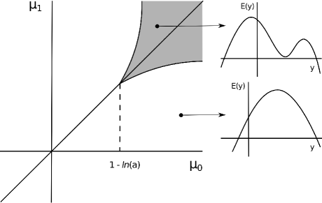
Figure 1. Phase diagram at fixed $a$

Points from the grayed area correspond to the existence of three solutions of (2.16), one of which is $y_{*}$. Note that $y_{*}>0$ for $\mu_{0}>\mu_{1}$. At the boundaries of this area (symmetric under $\mu_{0}\leftrightarrow\mu_{1}$), (2.16) has only two solutions. The upper branch of the boundary is described by the equation

$$\eta=\sqrt{\xi^{2}-1}+\ln\left(\xi-\sqrt{\xi^{2}-1}\right),$$ (2.24)

where $\xi=(\mu_{0}+\mu_{1})/2+\ln a$ and $\eta=(\mu_{1}-\mu_{0})/2$. The lower branch is given also by (2.24) with the same $\xi$ and $\eta=(\mu_{0}-\mu_{1})/2$. For all points from the complement to the grayed area, (2.16) has only one solution. Note that $y_{*}=0$ for $\mu_{0}=\mu_{1}<1-\ln a$.

2.2.2. The one-component model

In this case, the phase space is $\widehat{\mathcal{F}}=\{(a,\mu):a\geq 0,\mu\in\mathds{R}\}$, cf (2.5) and (2.9).

Theorem 2.3.

The phase space $\widehat{\mathcal{F}}$ can be divided into disjoint subsets $\widehat{\mathcal{R}}$, $\widehat{\mathcal{M}}$ and the critical point $(e/\theta,\ln\theta)$. Here $\widehat{\mathcal{M}}=\{(a,\mu):a>e/\theta,\mu=\ln\theta\}$ is the phase coexistence line and $\widehat{\mathcal{R}}$ is the single-phase domain. For each $(a,\mu)\in\widehat{\mathcal{R}}$, there exists a unique phase $P_{z}$ with activity $z=u(a,\mu+y_{*})$ where $y_{*}$ is the point of a unique global maximum of the function defined in (2.11) with $\mu_{0}=\mu$ and $\mu_{1}=\ln\theta$. For each $(a,\mu)\in\widehat{\mathcal{M}}$, there exist two phases: $P_{z^{+}}$ and $P_{z^{-}}$, where $z^{\pm}$ and the order parameter $\bar{y}$ are the same as in (2.19).

The proof of this theorem readily follows from Theorem 2.2. The density of the particles in state $P_{z}$ is $\varrho=z=u(a,\mu+y_{*})$; it depends also on $\theta$. Moreover, by (2.21) we have that $\varrho$ satisfies

$$\varrho=\exp\left(\mu-\theta e^{-a\varrho}\right).$$ (2.25)

It is an increasing and continuous function of $\mu$ whenever $a\leq e/\theta$. For $a>e/\theta$, $\varrho$ makes a jump at $\mu=\ln\theta$ with one-sided limits $\lim_{\mu\to\ln\theta\pm 0}\varrho=u(a,\mu\pm\bar{y}(a,\mu))$. That is, the system undergoes a first-order phase transition with the increment of the density $\varDelta\varrho=\bar{y}(a,\mu)/a$. The pressure defined in the second line of (2.7) is, cf (2.20),

$$\widehat{p}=\widehat{p}(a,\mu)=a\theta\varrho e^{-a\varrho}+\varrho-\theta\left(1-e^{-a\varrho}\right),$$ (2.26)

that can be obtained by (2.25) and the formula $\widehat{p}=p-\theta$. Its dependence on $\mu\in\mathds{R}$ comes only from the corresponding dependence of $\varrho$ just mentioned. In view of this, for a fixed $a$, $\widehat{p}$ can also be considered as a function of $\varrho$. This is typical for the corresponding works employing the canonical partition function calculated for a fixed number of particles $n$ in a vessel of volume $V$. Ten $\widehat{p}$ is obtained in the thermodynamic limit $n\to+\infty$, $V\to+\infty$, taken in such a way that $n/V\to\varrho$. In this case, the density appears as an independent parameter of the theory, see, e.g., [8, 1, 6]. The drawback of this way is that, for $a>e/\theta$, $\widehat{p}$ is a decreasing function of $\varrho$ on a subinterval of $[z^{-},z^{+}]$, which is impossible from the physical point of view. The correct form of this dependence can be deduced from the information on the dependence of $\varrho$ on $\mu$ discussed above. Namely, $\widehat{p}$ is given as in (2.26) for $\varrho\leq z^{-}$ and $\varrho\geq z^{+}$. On the interval $[z^{-},z^{+}]$ it is constant, i.e.,

$$\widehat{p}\equiv\widehat{p}_{*}:=az^{+}z^{-}+z^{+}+z^{-}-\theta.$$ (2.27)

In the canonical formalism, the horizontal part of the dependence of $\widehat{p}$ on $\varrho$ may be obtained from the Maxwell rule, cf [8]. To check whether this rule works in our case we have to show that the following holds

$$\int_{1/z^{+}}^{1/z^{-}}\left[\widehat{p}(1/v)-\widehat{p}_{*}\right]dv=0,$$ (2.28)

which is equivalent to, cf (2.27),

$$-\int_{z^{-}}^{z^{+}}\left[a\theta\varrho e^{-a\varrho}+\varrho+\theta e^{-a\varrho}\right]d\frac{1}{\varrho}=a\left(z^{+}-z^{-}\right)+\frac{z^{+}}{z^{-}}-\frac{z^{-}}{z^{+}}.$$ (2.29)

We take into account that $a\theta\varrho e^{-a\varrho}d\frac{1}{\varrho}=\frac{\theta}{\varrho}de^{-a\varrho}$, and then by integrating by parts we bring the left-hand side of (2.29) to the following form

$${\rm LHS}(\ref{U9})=\frac{\theta}{z^{-}}e^{-az^{-}}-\frac{\theta}{z^{+}}e^{-az^{+}}+\ln\frac{z^{+}}{z^{-}}.$$ (2.30)

Since $z^{\pm}=u(a,\mu\pm\bar{y}(a,\mu))$, by the first line in (2.15) it follows that

$$\frac{\theta}{z^{\pm}}e^{-az^{\pm}}=\theta e^{-\mu\mp\bar{y}(a,\mu)}=e^{\mp\bar{y}(a,\mu)},$$

where we have taken into account that $\mu=\ln\theta$ as $(a,\mu)\in\widehat{\mathcal{M}}$. Likewise, we have that $z^{+}/z^{-}=e^{\bar{y}(a,\mu)}$. On the other hand, by (2.16) it follows that $\bar{y}(a,\mu)=a(z^{+}-z^{-})$. We apply the latter three facts in (2.30) and obtain

$${\rm LHS}(\ref{U9})=e^{\bar{y}(a,\mu)}-e^{-\bar{y}(a,\mu)}+\bar{y}(a,\mu)=\frac{z^{+}}{z^{-}}-\frac{z^{-}}{z^{+}}+a(z^{+}-z^{-})={\rm RHS}(\ref{U9}),$$

which completes the proof of (2.28). Note that the equation of state in (2.26) with $a=1$ formally coincides with that found heuristically in [1].

3. Proving Theorem 2.2

We divide the proof into the following steps. First we prove Proposition 2.1 that relates the phase diagram (2.10) to the properties of the function $E$. Thereafter, we relate $E$ with the large $V$ asymptotic of $\ln\Xi_{\Lambda}/V$.

3.1. The proof of Proposition 2.1

By the very definition, see (2.11) – (2.15), it readily follows that $E$ is an infinitely differentiable function. To prove that it attains its global maxima not at infinity, let us show that

$$E(y)\to-\infty,\qquad{\rm as}\ \ |y|\to+\infty.$$ (3.1)

Since $E$ is symmetric with respect to the simultaneous interchange $y\leftrightarrow-y$ and $\mu_{0}\leftrightarrow\mu_{1}$, it is enough to prove (3.1) for $y\to+\infty$. By (2.14) we have

$$u(a,x) < \frac{x}{a}-\ell(a,x),\qquad x>a,$$ (3.2)

$$\ell(a,x) = \frac{1}{a}\ln\left(\frac{x}{a}-\frac{1}{a}\ln\frac{x}{a}\right).$$

Note that $\ell(a,x)>0$ for $x>a$ and $\ell(a,x)\to+\infty$ as $x\to+\infty$. On the other hand, since $u(a,x)>0$, for $x<0$ we have that $u(a,x)<e^{x}$ and hence $u(a,x)\to 0$ as $x\to-\infty$. By (2.15) we get that $u$ is an increasing function of $x$, which by (3.2) and (2.16) yields that $y>w(y)$ (resp. $y<w(y)$) for big enough $y$ (resp. $-y$). Thus (2.16) has at least one solution, say $y_{0}$. For $\mu_{0}=\mu_{1}$, $w(0)=0$; hence, this solution gets positive for $\mu_{0}>\mu_{1}$. By (2.11) and (2.16) we have that

$$E(y_{0})=\frac{a}{2}u(a,\mu_{0}+y_{0})u(a,\mu_{1}-y_{0})+u(a,\mu_{0}+y_{0})+u(a,\mu_{1}-y_{0})>0,$$ (3.3)

holding for all $y_{0}$ such that $w(y_{0})=y_{0}$.

By (3.2), (2.11) and (2.12) for $y>\max\{a-\mu_{0};\mu_{1}\}$ we obtain

$$E(y) < \frac{a}{2}\left(\frac{\mu_{0}+y}{a}-\ell(a,\mu_{0}+y)\right)^{2}+\frac{\mu_{0}+y}{a}-\ell(a,\mu_{0}+y)$$

$$+ \frac{a}{2}+1-\frac{y^{2}}{2a}=-A_{1}(y)y-A_{2}(y)\ell(a,\mu_{0}+y)+\frac{\mu_{0}^{2}}{2a}+\frac{a}{2}+1,$$

with

$$A_{1}(y)=\frac{1}{2}\ell(a,\mu_{0}+y)-\frac{\mu_{0}+1}{a},$$ (3.5)

$$A_{2}(y)=\frac{y}{2}-\frac{a}{2}\ell(a,\mu_{0}+y)+\mu_{0}+1.$$

Clearly, both these coefficients get positive for sufficiently big $y$, which by (3.1) yields (3.1). This means that the global maxima of $E$ are attained not at infinity and hence are also local maxima, cf (3.3). Therefore, the global maxima of this function are to be found by solving the equation in (2.16). Let us first consider the case where $\mu_{0}=\mu_{1}=\mu$. Then $w$ is an odd function and hence $y=0$ is a solution of (2.16). By (3.2) similarly as the estimate in (3.1) we obtain that $w(y)<y$ for sufficiently large $y$, and hence $w(y)-y$ is eventually negative. Obviously, the existence of positive solutions of (2.16) is determined by the slope of the curve $(w(y),y)$. This means that we have to study the dependence of $w^{\prime}(y)-1$ on $y$. By means of (2.15) we get that

$$w^{\prime}(y)-1 = \frac{c(y)}{[1+au(a,\mu+y)][1+au(a,\mu-y)]},$$ (3.6)

$$c(y) := a^{2}u(a,\mu+y)u(a,\mu-y)-1.$$

That is, the number of positive solutions of $w(y)=y$ coincides with that of $w^{\prime}(y)=1$, and thus of $c(y)=0$. We apply (2.15) once more and obtain

$$c^{\prime}(y)=\frac{a^{3}u(a,\mu+y)u(a,\mu-y)}{[1+au(a,\mu+y)][1+au(a,\mu-y)]}\left[u(a,\mu-y)-u(a,\mu+y)\right].$$ (3.7)

Since $u(a,\mu+y)$ is an increasing function of $y$, $c(y)$ has a unique maximum at $y=0$. By the analysis made above regarding the dependence of $u(a,x)$ on $x$ we conclude that $c(y)\to-1$ as $y\to\pm\infty$. This and (3.7) imply that $c$ has two real zeros, say $\pm\hat{y}$, $\hat{y}>0$, whenever $c(0)>0$. It has a single zero at $y=0$ if $c(0)=0$. If $c(0)<0$, then $c(y)<0$ for all real $y$. In view of (3.6), we then have the following options: (i) $c(0)>0$, and hence $w^{\prime}(0)>1$, which implies that $w(y)=y$ holds for $y=0$ and $y=\pm\bar{y}$, such that $\bar{y}\geq\hat{y}$; (ii) $c(0)=0$, and hence $w^{\prime}(0)=1$ and $w^{\prime}(y)<1$ for all $y>0$, which implies and $w(y)<y$ for all $y>0$; (iii) $c(0)<0$, and hence $w(y)<y$ for all $y>0$. Let us analyze these possibilities in terms of the parameters $\mu$ and $a$. In case (ii), we have $u(a,\mu)=1/a$, which by (2.15) yields $\mu=\mu_{c}:=1-\ln a$ that determines a critical point, cf (2.10). Since $c(0)$ is an increasing function of $\mu$, then $c(0)>0$ implies that $\mu>\mu_{c}$ that corresponds to case (i). Likewise, $\mu<\mu_{c}$ in case (iii). To relate this with $E$ we use the fact that $E^{\prime\prime}(y)=(w^{\prime}(y)-1)/a$, see (2.11), (2.12) and (2.16). Thus, in case (i), $E$ has two equal non-degenerate local (and also global) maxima at $\pm\bar{y}=\pm\bar{y}(a,\mu)$ and one local minimum at 0. In case (ii), $E$ has a degenerate maximum at 0. In case (iii), this unique maximum gets non-degenerate. This proves claim (b) of the statement, and the part of (a) corresponding to the case of equal $\mu_{i}$. Let us show that, for $y>0$, (2.16) turns into (2.17). To simplify notations by the end of this proof we set $v_{\pm}(y)=au(a,\mu\pm y)$. Then $v_{\pm}(y)\exp(v_{\pm}(y))=\exp(\mu+\ln a\pm y)$, see (2.15). We combine this with (2.16) in the form $y=v_{+}(y)-v_{-}(y)$ to obtain

$$v_{+}(y)=\frac{ye^{y}}{e^{y}-1},\quad v_{-}(y)=\frac{e^{y}}{e^{y}-1}.$$ (3.8)

Then we rewrite (2.14) in the form

$$\ln v_{-}(y)+v_{-}(y)+y-1=\mu-(1-\ln a),$$

that by (3.8) coincides with (2.17).

To complete the proof we have to consider the case of unequal $\mu_{i}$. In view of the mentioned symmetry of $E$, it is enough to consider the case $\mu_{0}\geq\mu_{1}$. Set $\mu_{1}=\mu$ and $\mu_{0}=\mu+\delta$, and then

$$w(\delta,y)=au(a,\mu+\delta+y)-au(a,\mu-y).$$ (3.9)

By (3.2) we have that $w(\delta,y)<y$ for sufficiently large $y$. At the same time, $w(\delta,0)>0$ for $\delta>0$. That is, (2.16) has at least one positive solution, say $y_{*}$, in this case. It is such that $E^{\prime\prime}(y_{*})=(w^{\prime}(y_{*})-1)/a<0$; i.e., $E$ has a non-degenerate maximum at $y_{*}$. By standard arguments based on the implicit function theorem we have that $y_{*}$ is a continuous function of $\delta\geq 0$ that tends to a nonnegative solution of (2.16) as $\delta\to 0^{+}$. Its $\delta$-derivative $\dot{y}_{*}$ can be calculated from the equality $y_{*}=w(\delta,y_{*})$, which yields

$$\dot{y}_{*}=\frac{au(a,\mu+\delta+y_{*})}{\left[1-w^{\prime}(\delta,y_{*})\right]\left[1+au(a,\mu+\delta+y_{*})\right]}>0.$$ (3.10)

That is, for $\mu\leq\mu_{c}$ and $\delta>0$, $y_{*}>0$ is the only maximum point of $E$, and $y_{*}\to 0$ as $\delta\to 0^{+}$. For $\mu>\mu_{c}$, by the positivity in (3.10) we have that $y_{*}>\bar{y}(a,\mu)$. In this case, we have two more solutions of $w(0,y)=y$. By the $\delta$-continuity of the solutions of $y=w(\delta,y)$ it should have two more solutions, say $y_{1}$ and $y_{0}$, close to $-\bar{y}(a,\mu)$ and zero, respectively, for small enough $\delta>0$. Their derivatives have the form as in (3.10) with $y_{*}$ replaced by the corresponding $y_{j}$. Since $w^{\prime}(\delta,y_{0})$ is close to $w^{\prime}(0,0)$, then $\dot{y}_{0}<0$, and hence $y_{0}<0$. At the same time, $\dot{y}_{1}>0$ for the same reason. That is, these two solutions move towards each other as $\delta$ increases. Let us compare the values of $E$ at $y_{*}$ and $y_{1}$. For $\delta=0$, we have that $E(y_{1})=E(y_{*})$. The $\delta$-derivative $\dot{E}(y)$ can be calculated from (2.11), which yields

$$\dot{E}(y)=u(a,\mu+\delta+y)+\dot{y}\left[w(\delta,y)-y\right]/a=u(a,\mu+\delta+y).$$

Here we have taken into account that $w(\delta,y)=y$ for $y=y_{1},y_{*}$. Thus, $\dot{E}(y_{*})>\dot{E}(y_{1})$ since $y_{*}>0>y_{1}$ and $u$ is an increasing function of $y$. This means that $y_{*}$ is the point of non-degenerate local and global maximum of $E$.

As follows from this proof, $y_{1}<y_{0}<0$ for $\mu>\mu_{c}$ and small $\delta>0$. Let us fix $\mu>\mu_{c}$ and find $\delta>0$ and $y<0$ such that $y_{1}=y_{0}=y$. Note that (2.16) has two solutions in this case: this $y$ and $y_{*}>0$. Clearly such $\delta$ and $y$ are to be found from the equation $w^{\prime}(\delta,y)=1$. Similarly as above, set $v_{+}(y)=au(a,\mu+\delta+y)$, $v_{-}(y)=au(a,\mu-y)$. Then $w^{\prime}(\delta,y)=1$ by (3.6) yields $v_{+}(y)v_{-}(y)=1$. By (2.15) we have

$$v_{+}(y)v_{-}(y)\exp\left[v_{+}(y)+v_{-}(y)\right]=\exp\left(2\mu+\delta+2\ln a\right),$$

by which we get

$$v_{+}(y)+v_{-}(y)=2\xi:=2\mu+\delta+2\ln a.$$ (3.11)

Since $y<0$, we have that $v_{+}(y)<v_{-}(y)$. Keeping this in mind we solve (3.11) and $v_{+}(y)v_{-}(y)=1$, which yields

$$v_{\pm}(y)=\xi\mp\sqrt{\xi^{2}-1},\quad y=-2\sqrt{\xi^{2}-1}.$$ (3.12)

By (2.15) we have

$$\frac{v_{+}(y)}{v_{-}(y)}\exp\left({v_{+}(y)}-{v_{-}(y)}\right)=\exp\left(2\eta+2y\right),\quad\eta:=\delta/2.$$

Now we use here (3.12) and arrive at (2.24).

3.2. Thermodynamics in a fixed vessel

In equilibrium statistical mechanics, the great canonical ensemble is determined by the family of local Gibbs measures indexed by all possible vessels $\Lambda$, see [9, Chapter 4]. Such measures are in turn uniquely determined by their correlation functions. For a given vessel $\Lambda$ and $x^{0}_{1},\dots,x^{0}_{n_{0}},x^{1}_{1},\dots,x^{1}_{n_{1}}\in\Lambda$, the correlation function $k^{(n_{0},n_{1})}_{\Lambda}(x_{1}^{0},\dots,x^{0}_{n_{0}};x_{1}^{1},\dots,x^{1}_{n_{1}})$ is defined as the density (with respect to the Lebesgue measure) of the probability distribution of the particles of both types in $\Lambda$. If the potential energy $\Phi_{\Lambda}$ is given, then

$$k^{(n_{0},n_{1})}_{\Lambda}(x_{1}^{0},\dots,x^{0}_{n_{0}};x_{1}^{1},\dots,x^{1}_{n_{1}})=\frac{1}{\Xi_{\Lambda}}\sum_{m_{0},m_{1}=0}^{\infty}\frac{z_{0}^{n_{0}+m_{0}}z_{1}^{n_{1}+m_{1}}}{m_{0}!m_{1}!}$$ (3.13)

$$\times\int_{\Lambda^{m_{0}}}\int_{\Lambda^{m_{1}}}\exp\left(-\Phi_{\Lambda}(x_{1}^{0},\dots,x^{0}_{n_{0}},y_{1}^{0},\dots,y^{0}_{m_{0}};x_{1}^{1},\dots,x^{1}_{n_{1}},y_{1}^{1},\dots,y^{1}_{m_{1}})\right)$$

$$\times dy_{1}^{0}\cdots,dy^{0}_{m_{0}}\cdot dy_{1}^{1}\cdots dy^{1}_{m_{1}},$$

where $z_{0}$, $z_{1}$ and $\Xi_{\Lambda}$ are the corresponding activities and the partition function, respectively. The correlation functions of the states of the whole infinite system can be obtained in the limit $\Lambda\to\mathds{R}^{d}$. For the Poissonian state defined in (2.1) and (2.2), we have that

$$k^{(n_{0},n_{1})}(x_{1}^{0},\dots,x^{0}_{n_{0}};x_{1}^{1},\dots,x^{1}_{n_{1}})=z_{0}^{n_{0}}z_{1}^{n_{1}},\qquad n_{0},n_{1}\in\mathds{N}_{0}.$$ (3.14)

Now for $\Phi_{\Lambda}$ as in (2.3) and fixed $\mu_{0}$, $\mu_{1}$, we thus have, cf (2.1) and (3.13),

$$k^{(n_{0},n_{1})}_{\Lambda}(x_{1}^{0},\dots,x^{0}_{n_{0}};x_{1}^{1},\dots,x^{1}_{n_{1}})=\exp\left(\mu_{0}n_{0}+\mu_{1}n_{1}-\frac{a}{V}n_{0}n_{1}\right)$$ (3.15)

$$\qquad\times\frac{1}{\Xi_{\Lambda}(a,\mu_{0},\mu_{1})}\sum_{m_{0},m_{1}=0}^{\infty}\frac{V^{m_{0}+m_{1}}}{m_{0}!m_{1}!}\exp\bigg{(}\left[\mu_{0}-\frac{a}{V}n_{1}\right]m_{0}$$

$$\qquad+\left[\mu_{1}-\frac{a}{V}m_{0}\right]m_{1}-\frac{a}{V}m_{0}m_{1}\bigg{)}$$

$$\qquad=\exp\left(\mu_{0}n_{0}+\mu_{1}n_{1}-\frac{a}{V}n_{0}n_{1}\right)\frac{\Xi_{\Lambda}(a,\mu_{0}-an_{1}/V,\mu_{1}-an_{0}/V)}{\Xi_{\Lambda}(a,\mu_{0},\mu_{1})}$$

Set

$$F_{\Lambda}(a,\mu_{0},\mu_{1}) = \frac{1}{V}\ln\Xi_{\Lambda}(a,\mu_{0},\mu_{1}),$$ (3.16)

$$F^{(i)}_{\Lambda}(a,\mu_{0},\mu_{1}) = \frac{\partial}{\partial\mu_{i}}F_{\Lambda}(a,\mu_{0},\mu_{1}),\quad i=0,1,$$

and rewrite (3.15) in the following form

$$k^{(n_{0},n_{1})}_{\Lambda}(x_{1}^{0},\dots,x^{0}_{n_{0}};x_{1}^{1},\dots,x^{1}_{n_{1}})=\exp\left(\tilde{\mu}^{\Lambda}_{0}n_{0}+\tilde{\mu}^{\Lambda}_{1}n_{1}-\frac{a}{V}n_{0}n_{1}\right),$$ (3.17)

with

$$\tilde{\mu}^{\Lambda}_{0}=\mu_{0}-a\int_{0}^{1}F^{(1)}_{\Lambda}\left(a,\mu_{0},\mu_{1}-\frac{a}{V}n_{0}t\right)dt,$$ (3.18)

$$\tilde{\mu}^{\Lambda}_{1}=\mu_{1}-a\int_{0}^{1}F^{(0)}_{\Lambda}\left(a,\mu_{0}-\frac{a}{V}n_{1}t,\mu_{1}-\frac{a}{V}n_{0}\right)dt.$$

Thus, we have to show that

$$\tilde{\mu}^{\Lambda}_{0}\to\ln\tilde{z}_{0}=\mu_{0}-au(a,\mu_{1}-y_{*}),$$ (3.19)

$$\tilde{\mu}^{\Lambda}_{1}\to\ln\tilde{z}_{1}=\mu_{1}-au(a,\mu_{0}+y_{*}),$$

as $V\to+\infty$, see (2.18), (2.21) and (3.14). This means that we have to obtain the large $V$ asymptotic of the functions defined in (3.16). To this end by means of the identity

$$-\frac{a}{V}n_{0}n_{1}=-\frac{a}{2V}n^{2}_{0}-\frac{a}{2V}n^{2}_{1}+\frac{a}{2V}(n_{0}-n_{1})^{2},$$

and then by the standard Gaussian formula

$$\exp\left(\frac{b^{2}}{2V}\right)=\sqrt{\frac{V}{2\pi}}\int_{-\infty}^{+\infty}\exp\left(by-\frac{Vy^{2}}{2}\right)dy,$$

we rewrite (2.1) and (3.16) in the form

$$\Xi_{\Lambda}(a,\mu_{0},\mu_{1})=\exp\left(VF_{\Lambda}(a,\mu_{0},\mu_{1}\right)=\sqrt{\frac{V}{2\pi}}\int_{-\infty}^{+\infty}\exp\left(VE_{V}(y)\right)dy,$$ (3.20)

with

$$E_{V}(y)=f_{V}(a,\mu_{0}+y)+f_{V}(a,\mu_{1}-y)-\frac{y^{2}}{2a}.$$ (3.21)

Here $f_{V}$ is defined by the following formula

$$\exp\left(Vf_{V}(a,x)\right)=\sum_{n=0}^{\infty}\frac{V^{n}}{n!}\exp\left(xn-\frac{a}{2V}n^{2}\right),$$ (3.22)

and thus is an infinitely differentiable function of $x\in\mathds{R}$ for each fixed $a>0$ and $V>0$. Then so is $E_{V}$ as a function of $y\in\mathds{R}$. Moreover, taking the $\mu_{i}$-derivatives of both sides of (3.20) we obtain

$$F^{(0)}_{\Lambda}(a,\mu_{0},\mu_{1})=\frac{\int_{-\infty}^{+\infty}u_{V}(a,\mu_{0}+y)\exp\left(VE_{V}(y)\right)dy}{\int_{-\infty}^{+\infty}\exp\left(VE_{V}(y)\right)dy},$$ (3.23)

$$F^{(1)}_{\Lambda}(a,\mu_{0},\mu_{1})=\frac{\int_{-\infty}^{+\infty}u_{V}(a,\mu_{1}-y)\exp\left(VE_{V}(y)\right)dy}{\int_{-\infty}^{+\infty}\exp\left(VE_{V}(y)\right)dy},$$

where, cf (3.22),

$$u_{V}(a,x)=\frac{\partial}{\partial x}f_{V}(a,x)=\frac{\langle n\rangle_{V}}{V}=\frac{1}{V}\sum_{n=1}^{\infty}n\pi_{V}(x,n),$$ (3.24)

$$\pi_{V}(x,n)=\frac{V^{n}}{n!}\exp\left(xn-\frac{a}{2V}n^{2}\right)\bigg{/}\sum_{n=0}^{\infty}\frac{V^{n}}{n!}\exp\left(xn-\frac{a}{2V}n^{2}\right).$$

To find the large $V$ asymptotic of the right-hand sides of (3.20) and (3.23) we employ a more advanced version of Laplace’s method as $E_{V}$ depends on $V$. Namely, we will use [12, Theorem 2.2, Chapter II] which we present here in the form adapted to the context.

Proposition 3.1.

Assume that, for all big enough $V$, the function defined in (3.21) has a unique non-degenerate global maximum at some $y_{*,V}\in\mathds{R}$, so that its second $y$-derivative satisfies $E^{\prime\prime}_{V}(y_{*,V})<0$. Assume also that there exists a function $V\mapsto\alpha_{V}>0$ such that $\alpha_{V}\to+\infty$ and

$$\Delta_{V}:=\frac{\alpha_{V}}{\sqrt{V|E^{\prime\prime}_{V}(y_{*,V})|}}\to 0,\quad{\rm as}\ \ V\to+\infty.$$ (3.25)

Set $U_{V}=[y_{*,V}-\Delta_{V},y_{*,V}+\Delta_{V}]$ and let $\phi_{V}(y)$ be constant or either of $u_{V}(a,\mu_{0}+y)$, $u_{V}(a,\mu_{1}-y)$, cf (3.23). Then in the limit of large $V$, it follows that

$$\int_{U_{V}}\phi_{V}(y)\exp\left(VE_{V}(y)\right)dy$$ (3.26)

$$\qquad\qquad=\sqrt{\frac{2\pi}{V|E^{\prime\prime}_{V}(y_{*,V})|}}\phi_{V}(y_{*,V})\exp\left(VE_{V}(y_{*,V})\right)\left[1+o(1)\right].$$

3.3. Preparatory statements

In this subsection, we obtain a number of results by means of which we then apply Proposition 3.1 in (3.23). We begin by obtaining some bounds on the first two $x$-derivatives of the function defined in (3.24) which we denote by $u^{\prime}_{V}(a,x)$ and $u^{\prime\prime}_{V}(a,x)$.

Lemma 3.2.

For each $x\in\mathds{R}$ and $V>0$, the following holds

$$0\leq u^{\prime}_{V}(a,x)\leq u_{V}(a,x).$$ (3.27)

Proof.

By taking the $x$-derivative in (3.24) we get

$$u^{\prime}_{V}(a,x)=\langle\left(n-\langle n\rangle_{V}\right)^{2}\rangle_{V}{/}V\geq 0,$$ (3.28)

which proves the lower bound stated in (3.27). On the other hand, by taking the $x$-derivative of both sides of (3.22) we obtain that $u_{V}$ satisfies, cf (2.15),

$$u_{V}(a,x)\exp\left(a\int_{0}^{1}u_{V}\left(a,x-\frac{a}{V}t\right)dt\right)=\exp\left(x-\frac{a}{2V}\right).$$ (3.29)

Now we differentiate both sides of (3.29) and obtain

$$u^{\prime}_{V}(a,x)+au_{V}(a,x)\int_{0}^{1}u^{\prime}_{V}\left(x-\frac{a}{V}t\right)dt=u_{V}(a,x).$$ (3.30)

In view of (3.28), the second summand here is positive which yields the upper bound in (3.27). ∎

Recall that $u(a,x)$ is defined in (2.13).

Corollary 3.3.

For each $x\in\mathds{R}$ and $V>0$, the following holds

$$u\left(a,x-\frac{a}{2V}\right)\leq u_{V}(a,x)\leq u\left(a,x+\frac{a}{2V}\right),$$ (3.31)

and hence

$$\left|u_{V}(a,x)-u(a,x)\right|\leq\frac{1}{2V}.$$ (3.32)

Proof.

By (3.27) $u_{V}\left(a,x\right)$ is an increasing function of $x$, which by (3.29) yields

$$u_{V}\left(a,x-\frac{a}{V}\right)\exp\left(au_{V}\left(a,x-\frac{a}{V}\right)\right)\leq\exp\left(x-\frac{a}{2V}\right),$$ (3.33)

$$u_{V}\left(a,x\right)\exp\left(au_{V}\left(a,x\right)\right)\geq\exp\left(x-\frac{a}{2V}\right).$$

On the other hand, by (2.15) we have that

$$\exp\left(x-\frac{a}{2V}\right)=u\left(a,x-\frac{a}{2V}\right)\exp\left(au\left(a,x-\frac{a}{2V}\right)\right).$$

Since the function $u\mapsto ue^{au}$ is increasing, the first line in (3.33) implies that

$$u_{V}\left(a,x-\frac{a}{V}\right)\leq u\left(a,x-\frac{a}{2V}\right),$$

which yields the upper bound in (3.31). The lower bound is obtained from the second line in (3.33) analogously. Then the estimate in (3.32) follows by these bounds and the fact that $u^{\prime}(a,x)\leq 1/a$, see (2.15). ∎

Lemma 3.4.

For each $a>0$, there exists a continuous function $x\mapsto h_{a}(x)>0$ such that, for all $V>0$, the following holds

$$\left|u^{\prime\prime}_{V}(a,x)\right|\leq h_{a}(x).$$ (3.34)

Proof.

Similarly as in (3.28) we get

$$u^{\prime\prime}_{V}(a,x)=\langle\left(n-\langle n\rangle_{V}\right)^{3}\rangle_{V}{/}V.$$ (3.35)

However, unlike to (3.28) we have no information on the sign of this derivative. The idea of proving (3.34) is to split $u^{\prime\prime}_{V}(a,x)$ into two parts, one of which is positive and the other one is controllable. Then the first part can be controlled similarly as in Lemma 3.2. To this end we use a certain property of the probability distribution defined in the second line of (3.24). Namely, we want to find its modes: all those $n_{*}$ that satisfy the conditions

$$\frac{\pi_{V}(a,n_{*}\pm 1)}{\pi_{V}(a,n_{*})}\leq 1.$$ (3.36)

By taking ‘minus’ in (3.36) we obtain from (3.24) and (2.15) that

$$\frac{n_{*}}{V}\exp\left(a\frac{n_{*}}{V}\right)\leq\exp\left(x+\frac{a}{2V}\right)=u\left(x+\frac{a}{2V}\right)\exp\left(au\left(x+\frac{a}{2V}\right)\right).$$ (3.37)

Likewise, by taking ‘plus’ in (3.36) we get

$$\frac{n_{*}+1}{V}\exp\left(a\frac{n_{*}+1}{V}\right)\geq\exp\left(x+\frac{a}{2V}\right).$$ (3.38)

Since the function $u\mapsto ue^{au}$ is increasing on $(0,+\infty)$, the inequalities and equalities in (3.37) and (3.38) imply that

$$Vu\left(x+\frac{a}{2V}\right)-1\leq n_{*}\leq Vu\left(x+\frac{a}{2V}\right),$$ (3.39)

and hence the probability distribution defined in the second line of (3.24) is unimodal. By (3.24) we have that $\langle n\rangle_{V}=Vu_{V}(a,x)$. Then we use the estimates in (3.31) and obtain from (3.39) the following

$$n_{*}-\langle n\rangle_{V}\leq V\left[u\left(x+\frac{a}{2V}\right)-u\left(x-\frac{a}{2V}\right)\right],$$

$$=\frac{a}{2}\int_{-1}^{1}u^{\prime}\left(a,x+\frac{a}{2V}t\right)dt\leq 1,$$

where we used the estimate $au^{\prime}(a,x)\leq 1$ which readily follows from the second line in (2.15). On the other hand, also by the estimates in (3.31) we get that $\langle n\rangle_{V}-n_{*}\leq 1$, which finally yields

$$\left|n_{*}-\langle n\rangle_{V}\right|\leq 1,$$ (3.40)

holding for all $x\in\mathds{R}$ and $V>0$. Now keeping in mind (3.35) we write

$$\langle\left(n-\langle n\rangle_{V}\right)^{3}\rangle_{V} = \langle\left(n-n_{*}+\frac{1}{2}\right)^{3}\rangle_{V}+3\left(n_{*}-\frac{1}{2}-\langle n\rangle_{V}\right)$$

$$\times \left[\langle\left(n-\langle n\rangle_{V}\right)^{2}\rangle_{V}+\left(n_{*}-\frac{1}{2}-\langle n\rangle_{V}\right)^{2}\right]-2\left(n_{*}-\frac{1}{2}-\langle n\rangle_{V}\right)^{3}$$

$$= \langle\left(n-n_{*}+\frac{1}{2}\right)^{3}\rangle_{V}+3\left(n_{*}-\frac{1}{2}-\langle n\rangle_{V}\right)\langle\left(n-\langle n\rangle_{V}\right)^{2}\rangle_{V}$$

$$+ \left(n_{*}-\frac{1}{2}-\langle n\rangle_{V}\right)^{3}.$$

Set

$$g_{V}(a,x)=\frac{1}{V}\langle\left(n-n_{*}+\frac{1}{2}\right)^{3}\rangle_{V}.$$ (3.42)

Then by (3.3) and (3.40) we have that

$$\left|u^{\prime\prime}_{V}(a,x)-g_{V}(a,x)\right|\leq\frac{9}{2}\left[u^{\prime}_{V}(a,x)+\frac{3}{4V}\right]$$ (3.43)

$$\leq\frac{9}{2}\left[u\left(a,x+\frac{a}{2V_{0}}\right)+\frac{3}{4V_{0}}\right]=:\chi(x),$$

where we assume that $V\geq V_{0}$ for some fixed $V_{0}$ and use the upper bounds in (3.27) and (3.31). To estimate $g_{V}$ we write

$$\langle\left(n-n_{*}+\frac{1}{2}\right)^{3}\rangle_{V} = \sum_{n=0}^{\infty}\left(n-n_{*}+\frac{1}{2}\right)^{3}\pi_{V}(x,n)$$

$$\geq \sum_{m=0}^{n_{*}-1}\left(m+\frac{1}{2}\right)\left(\pi_{V}(x,n_{*}+m)-\pi_{V}(x,n_{*}-m-1)\right).$$

By the second line in (3.24) we have

$$\frac{\pi_{V}(x,n_{*}+m)}{\pi_{V}(x,n_{*}-m-1)}$$

$$\qquad\qquad=\frac{V^{2m+1}\exp\left((2m+1)x-\frac{a}{2V}\left[(n_{*}+m)^{2}-(n_{*}-m-1)^{2}\right]\right)}{(n_{*}+m)(n_{*}+m-1)\cdots n_{*}\cdots(n_{*}-m+1)(n_{*}-m)}$$

$$\qquad\qquad=\left[\left(\frac{V}{n_{*}}\right)\exp\left(x-a\frac{n_{*}}{V}+\frac{a}{2V}\right)\right]^{2m+1}\bigg{/}\prod_{k=1}^{m}\left(1-\left(\frac{k}{n_{*}}\right)^{2}\right)\geq 1,$$

where the latter estimate follows by the inequality in (3.37). Then by (3.3) and (3.42) we conclude that, for all $x\in\mathds{R}$ and $V\geq V_{0}$,

$$g_{V}(x)\geq 0.$$ (3.45)

By (3.30) we get

$$a\int_{0}^{1}u^{\prime}_{V}\left(a,x-\frac{a}{V}t\right)dt=1-\frac{u^{\prime}_{V}(a,x)}{u_{V}(a,x)}.$$ (3.46)

Now we take the $x$-derivative of both sides of (3.30), use (3.46) and obtain

$$u^{\prime\prime}_{V}(a,x)+au_{V}(a,x)\int_{0}^{1}u^{\prime\prime}_{V}\left(a,x-\frac{a}{V}t\right)dt=\frac{\left[u^{\prime}_{V}(a,x)\right]^{2}}{u_{V}(a,x)}\leq u\left(a,x+\frac{a}{2V}\right),$$

where we also use the upper bounds in (3.27) and (3.31). We write here $u^{\prime\prime}_{V}=g_{V}+(u^{\prime\prime}_{V}-g_{V})$, use the estimate obtained in (3.43) and the positivity in (3.45). This yields

$$g_{V}(a,x)\leq g_{V}(a,x)+au_{V}(a,x)\int_{0}^{1}g_{V}\left(a,x-\frac{a}{V}t\right)dt$$ (3.47)

$$\leq u\left(a,x+\frac{a}{2V_{0}}\right)+\chi(x)+au\left(a,x+\frac{a}{2V_{0}}\right)\int_{0}^{1}\chi\left(x-\frac{a}{V_{0}}t\right)dt$$

$$\leq\chi(x)+u\left(a,x+\frac{a}{2V_{0}}\right)\left(1+a\chi(x)\right),$$

where we also use that $\chi$ is an increasing function, see (3.43) and (2.15). Thus, by the latter and (3.43) we conclude that the estimate stated in (3.34) holds true with $h_{a}=\chi+{\rm RHS}(\ref{L27})$. ∎

Corollary 3.5.

In the limit $V\to+\infty$, we have that $u^{\prime}_{V}\to u^{\prime}$ given in (2.15), point-wise in $a$ and uniformly on compact subsets of $\mathds{R}$ in $x$.

Proof.

We integrate by parts in (3.30) and obtain therefrom that

$$u^{\prime}_{V}(a,x)=\frac{u_{V}(a,x)}{1+au_{V}(a,x)}\left[1+\frac{a}{V}\int_{0}^{1}(1-t)u_{V}^{\prime\prime}\left(a,x-\frac{a}{V}t\right)dt\right].$$

Then the proof follows by (3.32), (3.34) and the fact that $u^{\prime}(a,x)=u(a,x)/(1+au(x,a))$, see (2.15). ∎

By (3.22) we have that $f_{V}(a,x)\leq e^{x}$ and hence $f_{V}(a,x)\to 0$ as $x\to-\infty$. By (3.24) this yields

$$f_{V}(a,x)=\int_{-\infty}^{x}u_{V}(a,y)dy,$$

which by (3.31) leads to

$$f\left(a,x-\frac{a}{2V}\right)\leq f_{V}(a,x)\leq f\left(a,x+\frac{a}{2V}\right).$$ (3.48)

Then for $V\geq V_{0}$, we have that

$$\left|f_{V}(a,x)-f(a,x)\right|\leq\frac{a}{2V}u\left(a,x+\frac{a}{2V_{0}}\right).$$ (3.49)

Lemma 3.6.

For each $a>0$, we have that $E_{V}\to E$ as $V\to+\infty$ uniformly on compact subsets of $\mathds{R}$. We also have that

$$E^{\prime}_{V}(y)\to E^{\prime}(y)=u(a,\mu_{0}+y)-u(a,\mu_{1}-y)-\frac{y}{a},$$ (3.50)

$$E^{\prime\prime}_{V}(y)\to E^{\prime\prime}(y)=\frac{u(a,\mu_{0}+y)}{1+au(a,\mu_{0}+y)}+\frac{u(a,\mu_{1}-y)}{1+au(a,\mu_{1}-y)}-\frac{1}{a},$$

where the convergence of the first (resp. second) derivatives is uniform (resp. uniform on compact subsets) in $y$.

Proof.

The convergence $E_{V}\to E$ follows by (3.49) and the fact that $f^{\prime}(a,x)=u(a,x)$ is bounded in $x$ on compact subsets of $\mathds{R}$. The uniform in $y$ convergence $E^{\prime}_{V}(y)\to E^{\prime}(y)$ follows by (3.32); the convergence of the second derivatives follows by Corollary 3.5. ∎

Lemma 3.7.

Assume that $(a,\mu_{0},\mu_{1})\in\mathcal{R}$, and hence the function $E$ defined in (2.11) has a unique non-degenerate global maximum at the corresponding $y_{*}\in\mathds{R}$, see Proposition 2.1. Then there exist $V_{0}>0$, $\varepsilon>0$ and $y_{\pm}$ such that $y_{-}<y_{+}$, $y_{*}\in[y_{-},y_{+}]$ and for all $V>V_{0}$ the following holds:

• the function $E_{V}$ defined in (3.21) has also a unique global maximum at some $y_{*,V}\in[y_{-},y_{+}]$;

• $-E^{\prime\prime}_{V}(y)\geq\varepsilon$ for all $y\in[y_{-},y_{+}]$;

• $y_{*,V}\to y_{*}$ as $V\to+\infty$.

Proof.

We begin by recalling that the assumptions imposed on $E$ imply that $E^{\prime\prime}(y_{*})<0$. Set, cf (3.9) and (3.50),

$$w(y)=au(a,\mu_{0}+y)-au(a,\mu_{1}-y)=aE^{\prime}(y)+y.$$ (3.51)

Then, cf (3.6),

$$w^{\prime}(y)-1 = \frac{c(y)}{[1+au(a,\mu_{0}+y)][1+au(a,\mu_{1}-y)]},$$ (3.52)

$$c(y) := a^{2}u(a,\mu_{0}+y)u(a,\mu_{1}-y)-1.$$

By (2.15) we get

$$c^{\prime}(y)=\frac{a^{3}u(a,\mu_{0}+y)u(a,\mu_{1}-y)}{[1+au(a,\mu_{0}+y)][1+au(a,\mu_{1}-)]}\left[u(a,\mu_{1}-y)-u(a,\mu_{0}+y)\right],$$ (3.53)

and hence $c^{\prime}(y)=0$ at $y=-(\mu_{0}-\mu_{1})/2$, where $c$ has maximum. since $E^{\prime\prime}(y_{*})<0$, we have that $w^{\prime}(y_{*})<1$ (see (3.51)), and hence

$$a^{2}u(a,\mu_{0}+y_{*})u(a,\mu_{1}-y_{*})-1<0.$$ (3.54)

Set,

$$w_{V}(y)=au_{V}(a,\mu_{0}+y)-au_{V}(a,\mu_{1}-y).$$ (3.55)

By (3.32) (resp. Corollary 3.5) it follows that $w_{V}\to w$ (resp. $w^{\prime}_{V}\to w^{\prime}$) as $V\to+\infty$, point-wise in $a$ and uniformly in $y$ (resp. uniformly in $y$ on compact subsets of $\mathds{R}$).

As above, we assume that $\mu_{0}\geq\mu_{1}$. For $\mu_{0}<\mu_{c}=1-\ln a$, we have that $w^{\prime}(y)<1$ for all $y\in\mathds{R}$, see Fig. 1, and hence $w(y)<y$ for all $y>y_{*}$, and $w(y)>y$ for all $y<y_{*}$. Fix any $y_{\pm}$ such that $y_{-}<y_{+}$ and $y_{*}\in[y_{-},y_{+}]$, then pick positive $V_{0}$ and $\varepsilon$ such that, for all $V>V_{0}$, the following holds: (a) $w_{V}(y_{+})<y_{+}$, $w_{V}(y_{-})>y_{-}$; (b) $1-w_{V}^{\prime}(y)\geq\varepsilon a$ for all $y\in[y_{-},y_{+}]$. This is possible in view of the convergence just mentioned. By (a) we then have that there exists a unique $y_{*,V}\in[y_{-},y_{+}]$ such that $w_{V}(y_{*,V})=y_{*,V}$ which is an extremum point of $E_{V}$. In view of the convergence stated in Lemma 3.6, this is the point of non-degenerate global maximum. By (b) we have that (ii) holds true. Thus, it remains to prove the validity of claim (iii) in this case. By the very definition of $y_{*}$ and $y_{*,V}$ we have that $y_{*}-y_{*,V}=w(y_{*})-w_{V}(y_{*,V})$. Then

$$|y_{*}-y_{*,V}|\leq|w(y_{*})-w_{V}(y_{*})|+|w_{V}(y_{*})-w_{V}(y_{*,V})|$$ (3.56)

$$\leq\frac{a}{V}+(1-a\varepsilon)|y_{*}-y_{*,V}|,$$

which yields $|y_{*}-y_{*,V}|<1/V\varepsilon$. Here we have taken in to account (3.32) and the fact that $y_{*},y_{*,V}\in[y_{-},y_{+}]$. Let us now consider the case $\mu_{0}>\mu_{c}$. Set $\delta=\mu_{0}-\mu_{1}$ and $\xi(\delta)=(\mu_{0}+\mu_{1})/2+\ln a=\mu_{0}-\mu_{c}+1+\delta/2$, $\eta(\delta)=\delta/2$. Let $\delta_{*}>0$ be defined by the condition that $\xi(\delta_{*})$ and $\eta(\delta_{*})$ satisfy (2.24). For $\delta\geq\delta_{*}$, $E$ has a single non-degenerate global maximum, and the proof of the lemma is the same as in the case of $\mu_{0}<\mu_{c}$. Thus, we ought to consider the case $\delta\in(0,\delta_{*})$ where $E$ has two local maxima, say at $y_{1}$ and $y_{*}>y_{1}$, and one local minimum at $y_{0}\in[y_{1},y_{*}]$, see Fig. 1 and Lemma 2.1. For $\mu_{0}>\mu_{1}$, $y_{*}$ is the point of non-degenerate global maximum of $E$. Since $c(y)$ defined in (3.52) is continuous, by (3.54) it follows that there exists $y_{-}\in(0,y_{*})$ such that $c(y_{-})<0$ and $w(y_{-})>y_{-}$. Note that $c(-\delta/2)>0$ for $\mu_{0}>\mu_{c}$. Set $2\varkappa=w(y_{-})-y_{-}$ and then pick $y_{+}>y_{*}$ such that $y_{+}-w(y_{+})\geq 2\varkappa$, which is possible in view of (3.2). By (3.53) we have that $c^{\prime}(y)<0$ for $y>0$; hence, $[y_{-},+\infty)\ni y\mapsto c(y)/(1+au(a,\mu_{1}-y))$ is a decreasing function. Thus, for all $y\in[y_{-},y_{+}]$, by (3.52) we have that

$$1-w(y)\geq 2a\varepsilon,$$ (3.57)

with

$$\varepsilon:=-\frac{c(y_{-})}{2a[1+au(a,\mu_{0}+y_{+})][1+au(a,\mu_{1}-y_{-})]}.$$

Then by the convergence of $w_{V}$ and $w^{\prime}_{V}$ discussed above, see (3.55), and (3.57 we conclude that there exists $V_{0}$ such that, for all $V>V_{0}$, the following holds: (a) $w_{V}(y_{-})-y_{-}\geq\varkappa$, and $y_{+}-w_{V}(y_{+})\geq\varkappa$; (b) $1-w_{V}(y)\geq a\varepsilon$ holding for all $y\in[y_{-},y_{+}]$. Thereafter, the proof of all the three claims of the lemma follows in the same way as in the case of $\mu_{0}<\mu_{c}$. ∎

Remark 3.8.

For $\mu_{0}\geq\mu_{1}$, we have that $-E^{\prime\prime}_{V}(y)>0$ for all $y>y_{*,V}$ and $V>V_{0}$. This can be seen from the fact that $w^{\prime}(y)-1$ vanishes just once for $y\geq y_{-}$ and from the convergence $w_{V}^{\prime}\to w^{\prime}$.

Finally, we study the thermodynamic limit for $(a,\mu_{0},\mu_{1})\in\mathcal{M}$, where $\mu_{0}=\mu_{1}=\mu>\mu_{c}=1-\ln a$, see (2.10), and thus $E_{V}$ is an even function, see (3.21). The proof of the next statement follows by the same arguments that were used in the proof of Lemma 3.7, case $\mu_{0}>\mu_{c}$.

Lemma 3.9.

Assume that $(a,\mu,\mu)\in\mathcal{M}$, and hence $E$ has two equal non-degenerate maxima at $\pm\bar{y}(a,\mu)$. Then there exist $V_{0}>0$, $\varepsilon>0$ and $\upsilon$ such that for all $V>V_{0}$ the following holds:

• there exists $y_{*,V}\in[\bar{y}(a,\mu)-\upsilon,\bar{y}(a,\mu)+\upsilon]$ such that $E_{V}(y_{*,V})\geq E_{V}(y)$ for all $y\geq 0$;

• $-E^{\prime\prime}_{V}(y)\geq\varepsilon$ for all $y\in[\bar{y}(a,\mu)-\upsilon,\bar{y}(a,\mu)+\upsilon]$;

• $y_{*,V}\to\bar{y}(a,\mu)$ as $V\to+\infty$.

3.4. The proof of Theorem 2.2

Basically, to complete the proof we have to show that: (a) the phases are as stated in claims (i) and (ii); (b) the following holds, cf (2.7), (2.20) and (3.20),

$$\lim_{V\to+\infty}F_{\Lambda}(a,\mu_{0},\mu_{1})=au(a,\mu_{0}+y_{*})u(a,\mu_{1}-y_{*})+u(a,\mu_{0}+y_{*})+u(a,\mu_{1}-y_{*}).$$ (3.58)

The proof of (a) will be done by showing the convergence stated in (3.19), which by (3.18) also amounts to studying the asymptotic properties of the integrals in (3.20) and (3.23). To this end we use Proposition 3.1, cf (3.26). First we consider the case $(a,\mu_{0},\mu_{1})\in\mathcal{R}$, see Lemma 3.7.

Lemma 3.10.

Assume that $(a,\mu_{0},\mu_{1})\in\mathcal{R}$ and let $y_{*,V}$ be as in Lemma 3.7. Then in the limit $V\to+\infty$ we have that

$$\int_{-\infty}^{+\infty}\phi_{V}(y)\exp\left(VE_{V}(y)\right)dy$$ (3.59)

$$\qquad\qquad=\sqrt{\frac{2\pi}{V|E^{\prime\prime}_{V}(y_{*,V})|}}\phi_{V}(y_{*,V})\exp\left(VE_{V}(y_{*,V})\right)\left[1+o(1)\right].$$

Proof.

Let $V_{0}$ and $\varepsilon$ be as in Lemma 3.7. Then $-E^{\prime\prime}(y_{*,V})\geq\varepsilon$ and hence $\Delta_{V}$ defined in (3.25) with $\alpha_{V}=V^{1/4}$ tends to zero. Let $I_{V}$ stand for the left-hand side of (3.26) with such $\Delta_{V}$. Let also $I^{-}_{V}$ and $I_{V}^{+}$ stand for the integrals over $(-\infty,y_{V}^{-}]$ and $[y_{V}^{+},+\infty)$, $y_{V}^{\pm}:=y_{*,V}\pm\Delta_{V}$, respectively, so that ${\rm LHS}(\ref{KL11})=I_{V}+I_{V}^{+}+I_{V}^{-}$. In view of Lemma 3.7, the proof of (3.59) will be done by showing that

$$I^{\pm}_{V}\exp\left(-VE_{V}(y_{*,V})\right)\to 0,\qquad{\rm as}\ \ V\to+\infty.$$ (3.60)

As above, we set $\mu_{0}\geq\mu_{1}$, and hence $y_{*,V}\geq 0$. Let $y_{\pm}$ be in Lemma 3.7. Since $\Delta_{V}\to 0$, we have that $y_{+}>y_{V}^{+}=y_{*,V}+\Delta_{V}$ and $y_{-}<y_{V}^{-}=y_{*,V}-\Delta_{V}$, holding for big enough $V$. By (3.2) and (3.5) both $A_{1}$ and $A_{2}$ in the estimate in (3.1) are increasing functions of $y$. Let $b_{+}>y_{+}$ (resp. $b_{-}<\min\{0;y_{-}\}$) and positive $C^{+}_{0},C_{1}^{+}$, $C^{+}_{0}<C_{1}^{+}b_{+}$ (resp. $C_{0}^{-},C_{1}^{-}$, $C_{0}^{-}<-C_{1}^{-}b_{-}$) be such that the following version of (3.1) holds

$$E(y)<\left\{\begin{array}[]{ll}C_{0}^{+}-C_{1}^{+}y,&{\rm for}\ \ y\geq b_{+};\\[5.69046pt] C_{0}^{-}+C_{1}^{-}y,&{\rm for}\ \ y\leq b_{-}.\end{array}\right.$$ (3.61)

By (3.48) we have that $E_{V}$ also satisfies (3.61) for all $V>V_{0}$. Since $y_{*,V}$ is neither in $[y_{+},b_{+}]$ nor in $[b_{-},y_{-}]$, there exists $\epsilon>0$ such that

$$E_{V}(y_{*,V})-\sup_{y\in[b_{-},y_{-}]}E_{V}(y)\geq\epsilon,\quad E_{V}(y_{*,V})-\sup_{y\in[y_{+},b_{+}]}E_{V}(y)\geq\epsilon.$$ (3.62)

Let $b_{\pm}$ be as just described. For all assumed choices of $\phi_{V}$, one can pick positive $c_{0}$, $c_{1}$ and $c_{2}$ such that:

$$\phi_{V}(y)\leq\left\{\begin{array}[]{ll}c_{0}+c_{1}y,&{\rm for}\ \ y\geq b_{+},\\[5.69046pt] c_{2},&{\rm for}\ \ y\in[b_{-},b_{+}]\\[5.69046pt] c_{0}-c_{1}y,&{\rm for}\ \ y\leq b_{-}.\end{array}\right.$$ (3.63)

Set

$$I^{+}_{V} = I^{+,0}_{V}+I^{+,1}_{V}+I^{+,2}_{V}$$

$$:= \int_{y_{V}^{+}}^{y_{+}}\phi_{V}(y)\exp\left(VE_{V}(y)\right)dy+\int_{y_{+}}^{b_{+}}\phi_{V}(y)\exp\left(VE_{V}(y)\right)dy$$

$$+ \int_{b_{+}}^{+\infty}\phi_{V}(y)\exp\left(VE_{V}(y)\right)dy.$$

By (3.61) and (3.63) we obtain

$$I^{+,2}_{V}\leq\exp\left(VC_{0}^{+}\right)\int_{b_{+}}^{\infty}(c_{0}+c_{1}y)\exp\left(-VC_{1}^{+}y\right)dy$$ (3.65)

$$=\frac{1}{C_{1}^{+}V}\exp\left(V[C_{0}^{+}-C_{1}^{+}b_{+}]\right)\left(c_{0}+c_{1}b_{+}+\frac{c_{1}}{C_{1}^{+}V}\right)$$

$$\leq\frac{1}{C_{1}^{+}V}\exp\left(VE_{V}(y_{*,V})\right)\left(c_{0}+c_{1}b_{+}+\frac{c_{1}}{C_{1}^{+}V}\right).$$

Here we have taken into account that $C_{0}^{+}-C_{1}^{+}b_{+}\leq 0$ and $E_{V}(y_{*,V})>0$, see (3.3) and (3.48).

To estimate $I^{+,1}_{V}$ we set $\epsilon_{V}^{+}=\sup_{y\in[y_{+},b_{+}]}E_{V}(y)$ and use the corresponding estimate from (3.63). By (3.62) this yields

$$I^{+,1}_{V}\leq c_{2}e^{V\epsilon_{V}^{+}}(b_{+}-y_{+})\leq c_{2}(b_{+}-y_{+})\exp\left(-V\epsilon+VE_{V}(y_{*,V})\right).$$ (3.66)

To estimate $I^{+,0}_{V}$ we use the fact that $-E^{\prime\prime}_{V}(y)\geq\varepsilon$ for all $y\in[y^{+}_{V},y_{+}]$. That is, $h_{V}(y):=-VE_{V}$ is convex and increasing on this interval. Set $\tau=h_{V}(y)$, and hence $dy=d\tau/h^{\prime}_{V}(y)$. Then, cf (3.63),

$$I^{+,0}_{V}=\int_{h_{V}(y_{V}^{+})}^{h(y_{+})}\frac{\phi_{V}(y)}{h^{\prime}_{V}(y)}e^{-\tau}dt\leq\frac{c_{2}}{V\varepsilon}\int_{h_{V}(y_{V}^{+})}^{h_{V}(y_{+})}e^{-\tau}d\tau$$ (3.67)

$$\leq\frac{c_{2}}{V\varepsilon}\exp\left(VE_{V}(y_{V}^{+})\right)\leq\frac{c_{2}}{V\varepsilon}\exp\left(VE_{V}(y_{*,V})\right).$$

Now we use (3.65), (3.66) and (3.67) in (3.4) and obtain that (3.58) holds true for $I^{+}_{V}$. Write

$$I^{-}_{V} = I^{-,0}_{V}+I^{-,1}_{V}+I^{-,2}_{V}$$

$$:= \int_{y_{-}}^{y_{V}^{-}}\phi_{V}(y)\exp\left(VE_{V}(y)\right)dy+\int_{b_{-}}^{y_{-}}\phi_{V}(y)\exp\left(VE_{V}(y)\right)dy$$

$$+ \int_{-\infty}^{b_{-}}\phi_{V}(y)\exp\left(VE_{V}(y)\right)dy,$$

where $y_{-}$ is the same as in Lemma 3.7 and $b_{-}$ as in (3.61). Then we proceed exactly as in (3.65), (3.66) and (3.67) to show that (3.60) holds true also for $I^{-}_{V}$. ∎

Now we consider the case where $(a,\mu,\mu)\in\mathcal{M}$ and thus $E_{V}$ is an even function, cf (3.21). In particular, $E_{V}(y_{*,V})=E_{V}(-y_{*,V})$.

Lemma 3.11.

Assume that $(a,\mu,\mu)\in\mathcal{M}$ and let $y_{*,V}$ be as in Lemma 3.9. Then in the limit $V\to+\infty$ we have that

$$\int_{-\infty}^{+\infty}\phi_{V}(y)\exp\left(VE_{V}(y)\right)dy$$ (3.68)

$$\qquad\qquad=\sqrt{\frac{2\pi}{V|E^{\prime\prime}_{V}(y_{*,V})|}}\left[\phi_{V}(-y_{*,V})+\phi_{V}(y_{*,V})\right]\exp\left(VE_{V}(y_{*,V})\right)\left[1+o(1)\right].$$

Proof.

Set

$$\varphi_{V}(y) = \phi_{V}(-y)+\phi_{V}(y),$$ (3.69)

$$I_{V} = \int_{0}^{+\infty}\varphi_{V}(y)\exp\left(VE_{V}(y)\right)dy.$$

Thus, we have to show that

$$I_{V}=\sqrt{\frac{2\pi}{V|E^{\prime\prime}_{V}(y_{*,V})|}}\varphi_{V}(y_{*,V})\exp\left(VE_{V}(y_{*,V})\right)\left[1+o(1)\right].$$ (3.70)

Let $V_{0}$, $\varepsilon$ and $\upsilon$ be as in Lemma 3.9 and $\Delta_{V}=V^{-1/4}/\sqrt{\varepsilon}$, cf (3.25). Set $y^{\pm}_{V}=y_{*,V}\pm\Delta_{V}$, $y_{\pm}=\bar{y}(a,\mu)\pm\upsilon$ and assume that $V$ is big enough so that $y_{-}<y^{-}_{V}$ and $y_{+}<y^{+}_{V}$. Let $C_{0}^{+}$, $C_{1}^{+}$ and $b_{+}$ be such that the first line in (3.61) holds true. We also assume that both estimates in (3.62) hold where $b_{-}$ is set to be zero. Finally, by (3.63) we have that

$$\varphi_{V}(y)\leq\left\{\begin{array}[]{ll}c_{2},&{\rm for}\ \ y\in[0,b_{+}];\\[5.69046pt] c_{0}+c_{1}y,&{\rm for}\ \ y>b_{+},\end{array}\right.$$ (3.71)

holding for all $V>V_{0}$. Then we split $I_{V}$ into six summands, i.e., write $I_{V}=\sum_{j=1}^{6}I_{j,V}$. In estimating these summands we mainly follow the way elaborated in proving Lemma 3.10. Namely, cf (3.66),

$$I_{1,V}:=\int_{0}^{y_{-}}\varphi_{V}(y)\exp\left(VE_{V}(y)\right)dy\leq c_{2}y_{-}\exp\left(-V\epsilon+VE_{V}(y_{*,V})\right).$$ (3.72)

Next, set $\tau=h_{V}(y):=-VE_{V}(y)$, cf (3.67),

$$I_{2,V}:=\int_{y_{-}}^{y^{-}_{V}}\varphi_{V}(y)\exp\left(VE_{V}(y)\right)dy=\int_{h_{V}(y_{-})}^{h_{V}(y_{V}^{-})}\frac{\varphi_{V}(y)}{h_{V}^{\prime}(y)}e^{-\tau}d\tau$$ (3.73)

$$\leq\frac{c_{2}}{V\varepsilon}\int_{h_{V}(y_{-})}^{h_{V}(y_{V}^{-})}e^{-\tau}d\tau\leq\frac{c_{2}}{V\varepsilon}\exp\left(VE_{V}(y_{V}^{-})\right)\leq\frac{c_{2}}{V\varepsilon}\exp\left(VE_{V}(y_{*,V})\right).$$

The next integral is estimated by means of Proposition 3.1. That is,

$$I_{3,V} := \int_{y_{V}^{-}}^{y_{V}^{+}}\varphi_{V}(y)\exp\left(VE_{V}(y)\right)dy$$

$$= \sqrt{\frac{2\pi}{V|E^{\prime\prime}_{V}(y_{*,V})|}}\varphi_{V}(y_{*,V})\exp\left(VE_{V}(y_{*,V})\right)\left[1+o(1)\right].$$

The next one is estimated pretty similar to (3.73)

$$I_{4,V} := \int_{y_{V}^{+}}^{y_{+}}\varphi_{V}(y)\exp\left(VE_{V}(y)\right)dy$$

$$\leq \frac{c_{2}}{V\varepsilon}\exp\left(VE_{V}(y_{V}^{+})\right)\leq\frac{c_{2}}{V\varepsilon}\exp\left(VE_{V}(y_{*,V})\right).$$

The next integral in turn is estimated similarly as in (3.72)

$$I_{5,V}:=\int_{y_{+}}^{b_{+}}\varphi_{V}(y)\exp\left(VE_{V}(y)\right)dy\leq c_{2}(b_{+}-y_{+})\exp\left(-V\epsilon+VE_{V}(y_{*,V})\right).$$ (3.76)

Finally, cf (3.65) and (3.71),

$$I_{6,V} := \int_{g_{+}}^{+\infty}\varphi_{V}(y)\exp\left(VE_{V}(y)\right)dy$$

$$\leq \exp\left(VC_{0}^{+}\right)\int_{g_{+}}^{+\infty}\left(c_{0}+c_{1}y\right)\exp\left(-VC_{1}^{+}y\right)dy$$

$$\leq \frac{1}{C_{1}^{+}V}\exp\left(VE_{V}(y_{*,V})\right)\left[c_{0}+c_{1}b_{+}+\frac{c_{1}}{C_{1}^{+}V}\right].$$

Now by (3.72), (3.73), (3.4), (3.4), (3.76) and (3.4) we conclude that (3.70) holds true. ∎

Proof of Theorem 2.2. First we consider the case $(a,\mu_{0},\mu_{1})\in\mathcal{R}$. Apply Lemma 3.10 in (3.23) with $\phi_{V}(y)=u_{V}(a,\mu_{0}+y)$ in the numerator and $\phi_{V}(y)\equiv 1$ in the denominator. This yields

$$F^{(0}_{\Lambda}(a,\mu_{0},\mu_{1})=u_{V}(a,\mu_{0}+y_{*,V})\left[1+o(1)\right].$$ (3.78)

On the other hand, by (3.32) and (3.56) we obtain

$$u_{V}(a,\mu_{0}+y_{*,V})=u(a,\mu_{0}+y_{*})+o(1)$$

Since $y_{*}$ is a continuously differentiable function of $\mu_{0}$ and $\mu_{1}$, cf (3.10), we have that

$$F^{(0}_{\Lambda}\left(a,\mu_{0}-\frac{a}{V}n_{1}t,\mu_{1}-\frac{a}{V}n_{0}\right)=u(a,\mu_{0}+y_{*})+o(1),$$

uniformly in $t\in[0,1]$. We use this in (3.18) and obtain that the second line in (3.19) holds true. The proof of the first line follows analogously. This proves claim (i) of the theorem. Let us now turn to the case $(a,\mu,\mu)\in\mathcal{M}$. By Lemma 3.11 we obtain, cf (3.78) and (3.69),

$$F^{(0}_{\Lambda}(a,\mu_{0},\mu_{1})=\frac{1}{2}\left[u_{V}(a,\mu-y_{*,V})+u_{V}(a,\mu+y_{*,V})\right](1+o(1)).$$ (3.79)

On the other hand, by (2.1) and then by (3.16) it follows that

$$F^{(0}_{\Lambda}(a,\mu_{0},\mu_{1}) = \varrho_{0,\Lambda}:=\frac{1}{\Xi_{\Lambda}(a,\mu_{0},\mu_{1})}$$

$$\times \sum_{n_{0},n_{1}=0}^{\infty}\left(\frac{n_{0}}{V}\right)\frac{V^{n_{0}+n_{1}}}{n_{0}!n_{1}!}\exp\left(\mu_{0}n_{0}+\mu_{1}n_{1}-\frac{a}{V}n_{0}n_{1}\right).$$

That is, $F^{(0}_{\Lambda}(a,\mu_{0},\mu_{1})$ is the density of the particles of type 0 in the local state corresponding to the interaction energy (2.3) (determined by $a$) and chemical potentials $\mu_{0}$ and $\mu_{1}$. By (3.79) we have

$$\lim_{\Lambda\to\mathds{R}^{d}}\varrho_{0,\Lambda}=\frac{1}{2}\left[u(a,\mu-\bar{y}(a,\mu))+u(a,\mu+\bar{y}(a,\mu))\right].$$ (3.80)

Likewise,

$$\lim_{\Lambda\to\mathds{R}^{d}}\varrho_{1,\Lambda}={\rm RHS}(\ref{L52}),$$

and

$$\lim_{\Lambda\to\mathds{R}^{d}}F^{(01)}_{\Lambda}(a,\mu_{0},\mu_{1}) = \frac{1}{2}\bigg{(}u(a,\mu-\bar{y}(a,\mu))u(a,\mu+\bar{y}(a,\mu))$$

$$+ u(a,\mu+\bar{y}(a,\mu))u(a,\mu-\bar{y}(a,\mu))\bigg{)},$$

where

$$F^{(01)}_{\Lambda}(a,\mu_{0},\mu_{1}) = \frac{1}{\Xi_{\Lambda}(a,\mu_{0},\mu_{1})}$$

$$\times \sum_{n_{0},n_{1}=0}^{\infty}\left(\frac{n_{0}}{V}\right)\cdot\left(\frac{n_{1}}{V}\right)\frac{V^{n_{0}+n_{1}}}{n_{0}!n_{1}!}\exp\left(\mu_{0}n_{0}+\mu_{1}n_{1}-\frac{a}{V}n_{0}n_{1}\right).$$

That is, the limiting state in this case is the symmetric mixture (convex combination with equal coefficients) of two pure states (phases, see [10, Chapter 7]), say $P^{\pm}$. The particle densities $\varrho_{i}^{\pm}$ in these phases are

$$\varrho_{0}^{\pm}=u(a,\mu\pm\bar{y}(a,\mu)),\qquad\varrho_{1}^{\pm}=u(a,\mu\mp\bar{y}(a,\mu)).$$

For these phases, like in the case of $\mu_{0}\neq\mu_{1}$ we get, see (3.18) and (3.19), that

$${\rm for}\ P^{+}\ \ \tilde{\mu}_{0}^{\Lambda}\to\mu-u(a,\mu-\bar{y}(a,\mu))=\ln\tilde{z}^{+},\quad\ \tilde{\mu}_{1}^{\Lambda}\to\mu-u(a,\mu+\bar{y}(a,\mu))=\ln\tilde{z}^{-},$$

$${\rm for}\ P^{-}\ \ \tilde{\mu}_{0}^{\Lambda}\to\mu-u(a,\mu+\bar{y}(a,\mu))=\ln\tilde{z}^{-},\quad\ \tilde{\mu}_{1}^{\Lambda}\to\mu-u(a,\mu-\bar{y}(a,\mu))=\ln\tilde{z}^{+}.$$

By (3.17) and (3.14) this yields that $P^{+}=P_{\tilde{z}^{+},\tilde{z}^{-}}$ and $P^{-}=P_{\tilde{z}^{-},\tilde{z}^{+}}$, which proves claim (ii). To prove claim (iii) we use the first line in (2.7) and then (3.59) (resp. (3.68)) with $\phi_{V}\equiv 1$ for $\mu_{0}>\mu_{1}$ (resp. $\mu_{0}=\mu_{1}$). In both cases, by (3.3) this leads to (2.20). $\square$