Transitioning scenario of Bianchi-I universe within $f\left(R,T\right)$ formalism

Abstract

In this paper, we report the existence of transitioning scenario of Bianchi type I universe in the context of $f\left(R,T\right)$ gravity with special case $f\left(R,T\right)=f_{1}(R)+f_{2}(R)f_{3}(T)$ and it’s functional forms $f_{1}(R)=f_{2}(R)=R$ and $f_{3}(T)=\alpha T$ with $\alpha$ being constant. The exact solution of the Einstein’s field equations are derived by using the generalized hybrid expansion law that yields the model of transitioning universe from early deceleration phase to current acceleration phase. Under this specification, we obtain the singular as well as non singular solution of Bianchi type I model depending upon the particular choice of the value of problem parameters. We also notice that the validation of weak energy condition and dominant energy condition and violation of strong energy condition occurs for these values of problem parameters. The deceleration parameter is found to be negative at present (z = 0) in the derived model which is supported by recent observations.

I Introduction

In order to explain the cosmic acceleration, $f(R,T)$ theory of gravity Harko/2011 are an optimistic alternative of general relativity with cosmological constant $(\Lambda)$ because GR with $(\Lambda)$ faces some problems on theoretical ground like cosmic coincidence and fine tuned. The Refs. Riess/1998 ; Perlmutter/1999 have evidence that the model of accelerating universe without cosmological constant $(\Lambda)$ is possible only when about $95\%$ energy/matter contents of the present universe is in the form of dark energy/matter Kumar/2017 . However the nature of dark energy/matter is still dubious Dil/2017 ; Behrouz/2017 ; Germani/2017 ; Jennen/2016 . In $f(R,T)$ gravity, the matter Lagrangian is coupled with Ricci scalar $(R)$ and trace of energy momentum tensor $(T)$ Yadav/2014 ; Moraes/2017 ; Yadav/2018 . The $T$ - dependence $f(R,T)$ gravity leads to the possibilities of consideration of quantum effects that yields the probabilities of production of particles Parker/2014 . Such possibilities may give a clue that there is a connection between quantum theory of gravity and extended theory of gravity with matter-geometry coupling.

Despite of recent elaboration, the $f(R,T)$ theory of gravitation has already been applied in Astrophysics Zubair/2016 ; Yousaf/2017 ; Moraes/2017r ; MoraesSahoo/2017 ; Das/2016 ; Sharif/2014 as well as in Cosmology Yadav/2014 ; Yadav/2015 ; Yadav/2018 ; Moraes/2017 ; Myrazakulov/2012 ; Singh/2015 . Shabani and Farhoudi Shabani/2014 have deliberated the cosmological and solar system consequences of $f(R,T)$ gravity model. The Refs. Shabani/2014 deals with parametrized post-Newtinian parameter for $f(R,T)$ theory of gravitation and shows that this model may accept admissible values of parametrized post-Newtinian parameter especially 1 in case of $f(R,T)=f_{1}(R)+f_{2}(T)$. In the recent past, Kiani and Nozari Kiani/2014 have studied $f(R,T)$ model based on the scalar perturbation in the space-time. In Zubair/2016 ; Yousaf/2017 ; Moraes/2017 ; MoraesSahoo/2017 the authors have investigated wormhole solution in $f(R,T)$ gravity. Moraes and Sahoo Moraes/2017 have deliberated non-minimal matter-geometry coupling, governed by hybrid expansion law for isotropic and homogeneous universe. Our main goal in the present paper is to develop the anisotropic non-minimal matter geometry coupling in $f(R,T)$ theory of gravity by taking into account the generalized hybrid expansion law Yadav/2013 ; Ozgur/2014 that generates transitioning model of universe and describes both the early decelerated phase and present accelerated phase of universe expansion as well as transition between these two regimes. Shen and Zhao Shen/2014 have studied quintom model of universe in $f(R,T)$ gravity which gives the periodic varyiation of deceleration parameter. In the Ref. Aygun/2016 , the authors have elaborated the the idea of accelerating universe without attribution of dark energy/dark mater in $f(R,t)$ theory of gravitation and show that the acceleration is the geometrical property of the present universe. Recently, Moraes et al Moraes/2017a have searched a cosmological scenario from the Starobinsky model with in the framework of $f(R,T)=R+\alpha R^{2}+2\gamma T$ formalism with $\alpha$ and $\gamma$ being constant. In the present paper we will focus our attention on $f(R,T)=f_{1}(R)+f_{2}(R)f_{3}(T)$ gravity which has shown to provide an alternative to the cosmological issues like cosmic coincidence and fine tune in general theory of relativity. Also, the Refs. Moraes/2017 ; Zaregonbadi/2016 give an evidence that $f(R,T)$ gravity does not need to invoke the dark energy/dark matter for acceleration.

A Bianchi type I universe is the simplest and straightforward generalization of FRW universe because it describes homogeneous and anisotropic universe with different scale factors along each spatial directions. Despite of recent elaboration, in the literature, several authors have studied Bianchi type I model in different physical contexts Akarsu/2010 ; Kumar/2011 ; Yadav/2012 ; Saha/2004 ; Yadav/2016 . In the present paper, we confine ourselves to study the non-minimal matter geometry coupling governed by generalized hybrid expansion law within $f\left(R,T\right)$ formalism . The paper is organized as follow: in section 2, we formulate basic mathematical formalism of $f\left(R,T\right)=f_{1}(R)+f_{2}(R)f_{3}(T)$ gravity with specific choice i.e. $f_{1}(R)=f_{2}(R)=R$ and $f_{3}(T)=\alpha T$. In section 3, we have computed the field equations for $f\left(R,T\right)=R+\alpha RT$ theory of gravitation in Bianchi type I space-time. The physical consequences of the derived model and energy conditions have been discussed in section 4. In section 5, we have concluded our results.

II The $f\left(R,T\right)=f_{1}(R)+f_{2}(R)f_{3}(T)$ Gravity

The $f\left(R,T\right)$ theory of gravity is the modification of general relativity (GR). The action for $f(R,T)$ theory is given by Harko/2011 ; Yadav/2014 :

$$S=\int\sqrt{-g}\left(\frac{f(R,T)}{16\pi G}+L_{m}\right)dx^{4},$$ (1)

where $f\left(R,T\right)$ is an arbitrary function of the Ricci scalar $R$ and the trace $T$ of energy momentum tensor $T_{ij}$ while $L_{m}$ is the usual matter Lagrangian.
The energy momentum tensor $T_{ij}$ is read as

$$T_{ij}\,=\,-\frac{2}{\sqrt{-g}}\,\frac{\delta\left(\sqrt{-g}\,L_{m}\right)}{\delta g^{ij}}$$ (2)

The gravitational field of $f(R,T)$ gravity is given by

$$\begin{array}[]{ll}\left[f_{1}^{\prime}(R)+f_{2}^{\prime}(R)f_{3}^{\prime}(T)\right]R_{ij}-\frac{1}{2}f_{1}^{\prime}(R)g_{ij}+\left(g_{ij}\bigtriangledown^{i}\bigtriangledown_{i}-\bigtriangledown_{i}\bigtriangledown_{j}\right)\\ \\ \,\,\,\,\,\,\,\times\left[f_{1}^{\prime}(R)+f_{2}^{\prime}(R)f_{3}^{\prime}(T)\right]=\left[8\pi+{f_{2}}^{\prime}(R){f_{3}}^{\prime}(T)\right]T_{ij}+\\ \\ \,\,\,\,\,\,\,\,\,\,f_{2}(R)\left[f_{3}^{\prime}(T)p+\frac{1}{2}f_{3}(T)\right]g_{ij}\end{array}$$ (3)

Here, $f(R,T)=f_{1}(R)+f_{2}(R)f_{3}(T)$ and primes denote derivatives with respect to the arrangement. We assume $f_{1}(R)=f_{2}(R)=R$ and $f_{3}(T)=\alpha T$, with $\alpha$ as a constant Moraes/2017 .
Thus the equation (3) yields

$$G_{ij}=8\pi T^{(eff)}_{ij}=8\pi(T_{ij}+T^{(DE)}_{ij})$$ (4)

where, $T^{(eff)}_{ij}$, $T_{ij}$ and $T^{(DE)}_{ij}$ represent the effective energy momentum tensor, matter energy momentum tensor and dark energy term respectively. The dark energy term is read as

$$T^{(DE)}_{ij}=\frac{\alpha R}{8\pi}\left(T_{ij}+\frac{3\rho-7p}{2}g_{ij}\right).$$ (5)

It is worth to note that the term $T^{(DE)}_{ij}$ arises due the matter-energy coupling in present theory Moraes/2017 .
By applying the Bianchi identities in equation (4) yields

$$\bigtriangledown^{i}T_{ij}=-\frac{\alpha R}{8\pi}\left[\bigtriangledown^{i}(T_{ij}+pg_{ij})+\frac{1}{2}g_{ij}\bigtriangledown^{i}(\rho-3p)\right]$$ (6)

III The metric and field equations

The line element of Bianchi type I space-time is read as

$$ds^{2}=dt^{2}-A^{2}\,dx^{2}-B^{2}\,dy^{2}-C^{2}\,dz^{2},$$ (7)

where $A=A(t)$, $B=B(t)$ and $C=C(t)$ are functions of $t$ only.

Figure 1: Variation of $\rho^{(eff)}$ (left panel) and $~{}p^{(eff)}$ (right panel) versus time for $b_{1}=.3$, $b_{2}=.7$, $b_{3}=-1$, $\lambda=0.25$, $m=1.25$, $n=0.75$.

Figure 2: The behavior of deceleration parameter (left panel) and $\omega^{\;eff}$ (right panel) versus time for $b_{1}=.3$, $b_{2}=.7$, $b_{3}=-1$, $\lambda=0.25$, $m=1.25$, $n=0.75$.

Figure 3: Validation of WEC for $b_{1}=.3$, $b_{2}=.7$, $b_{3}=-1$, $\lambda=0.25$, $m=1.25$, $n=0.75$

Figure 4: Validation of DEC for $b_{1}=.3$, $b_{2}=.7$, $b_{3}=-1$, $\lambda=0.25$, $m=1.25$, $n=0.75$

Figure 5: Violation of SEC for $b_{1}=.3$, $b_{2}=.7$, $b_{3}=-1$, $\lambda=0.25$, $m=1.25$, $n=0.75$

Figure 6: Evolution of DP with $z$ for different values of $\lambda$ and $n$.

Figure 7: Variation of $\triangle$ (left panel), $\theta$ (upper right panel), $\sigma^{2}$ (lower left panel) and $H$ (lower right panel) versus time for $b_{1}=.3$, $b_{2}=.7$, $b_{3}=-1$, $\lambda=0.25$, $m=1.25$, $n=0.75$.

The line-element (7) and field equation (2) lead the following equations:

$$\frac{\ddot{B}}{B}+\frac{\ddot{C}}{C}+\frac{\dot{B}\dot{C}}{BC}=-8\pi p^{(eff)}$$ (8)

$$\frac{\ddot{C}}{C}+\frac{\ddot{A}}{A}+\frac{\dot{A}\dot{C}}{AC}=-8\pi p^{(eff)}$$ (9)

$$\frac{\ddot{A}}{A}+\frac{\ddot{B}}{B}+\frac{\dot{A}\dot{B}}{AB}=-8\pi p^{(eff)}$$ (10)

$$\frac{\dot{A}\dot{B}}{AB}+\frac{\dot{B}\dot{C}}{BC}+\frac{\dot{C}\dot{A}}{CA}=8\pi\rho^{(eff)}$$ (11)

Here, $\rho^{(eff)}=\rho+\rho^{(DE)}=\rho-\frac{3\alpha}{8\pi}\left(\frac{\ddot{a}}{a}+\frac{\dot{a}^{2}}{a^{2}}\right)(3\rho-7p)$, $p^{(eff)}=p+p^{(DE)}=p+\frac{9\alpha}{8\pi}\left(\frac{\ddot{a}}{a}+\frac{\dot{a}^{2}}{a^{2}}\right)(\rho-3p)$ and $a=(ABC)^{\frac{1}{3}}$ is average scale factor.

The above equations (8)$-$(11) can also be written as

$$\frac{(ABC)^{\ddot{}}}{ABC}=12\pi(\rho^{(eff)}-p^{(eff)})$$ (12)

III.1 Solution of field equations & physical parameters

The generalized HEL form of scale factor Ozgur/2014 ; Yadav/2013 ; Yadav/2016 is given by

$$a=[t^{n}exp(\lambda t)]^{\frac{1}{m}}$$ (13)

where, $m$, $n$ and $\lambda$ are positive constants.

Solving equations (8)$-$(11) with equation (13), we obtain

$$A(t)=a_{1}[t^{n}exp(\lambda t)]^{\frac{1}{m}}exp\left[b_{1}\int\left(t^{n}exp(\lambda t)\right)^{-\frac{3}{m}}dt\right]$$ (14)

$$B(t)=a_{2}[t^{n}exp(\lambda t)]^{\frac{1}{m}}exp\left[b_{2}\int\left(t^{n}exp(\lambda t)\right)^{-\frac{3}{m}}dt\right]$$ (15)

$$C(t)=a_{3}[t^{n}exp(\lambda t)]^{\frac{1}{m}}exp\left[b_{3}\int\left(t^{n}exp(\lambda t)\right)^{-\frac{3}{m}}dt\right]$$ (16)

where $a_{1}$, $a_{2}$, $a_{3}$, $b_{1}$, $b_{2}$ & $b_{3}$ are constants that fulfill the following requirements:
$a_{1}a_{2}a_{3}=1$ & $b_{1}+b_{2}+b_{3}=0$.
The deceleration parameter of derived model is given by

$$q=\frac{mn}{(n+\lambda t)^{2}}-1$$ (17)

Solving equations (8)$-$(11) and (14)$-$(16), the expressions for $\rho^{(eff)}$ and $p^{(eff)}$ are respectively read as

$$\begin{array}[]{ll}8\pi\rho^{(eff)}=\frac{3}{m^{2}}\left(\lambda+\frac{m}{t}\right)^{2}+(b_{1}b_{2}+b_{2}b_{3}+b_{3}b_{1})\times\\ \\ \,\,\,\,\,\,\,\,\,\,\,\,\,\,\,\,\,\,\,\,\,\,\,\,\,\,\,\,\,\,\,\,\,\,\,\,\,\,\,\,[t^{n}exp(\lambda t)]^{-\frac{6}{m}}.\end{array}$$ (18)

$$\begin{array}[]{ll}8\pi p^{(eff)}=\frac{6b_{1}}{m}(t^{n}exp(\lambda t)^{-\frac{3}{m}}\left[3(\lambda+\frac{m}{t})-3t^{3}exp(\lambda t)\right]\\ \\ \,\,\,\,\,\,\,\,\,\,-(b_{1}b_{2}+b_{2}b_{3}+b_{3}b_{1})[t^{n}exp(\lambda t)]^{-\frac{6}{m}}+\frac{2n}{mt^{2}}\\ \\ \,\,\,\,\,\,\,\,\,\,\,\,\,\,\,\,\,\,\,\,\,\,\,\,\,\,\,-\frac{3}{m^{2}}\left(\lambda+\frac{m}{t}\right)^{2}.\end{array}$$ (19)

IV Physical consequences of the model & energy conditions

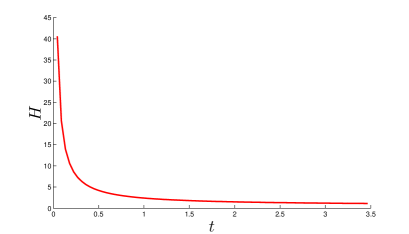
We observe that the equations (14)$-$(19), identically satisfy equation (12). Hence the solutions obtained in this paper are exact as well as important for describing the dynamics of physical universe. The Hubble’s parameter is computed as $H=\frac{3}{m}\left(\frac{n}{t}+\lambda\right)$. In the derived model, it has been seen also seen that the expansion scalar $(\theta)$ is proportional to Hubble’s parameter $(H)$ and $V=a^{3}$.
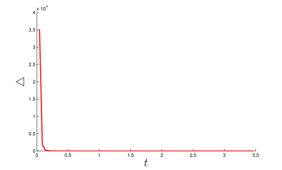
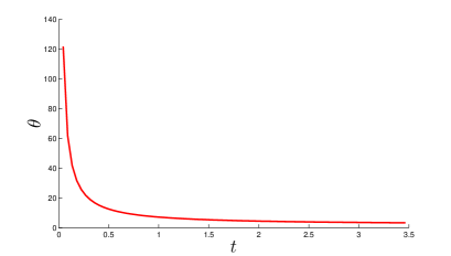
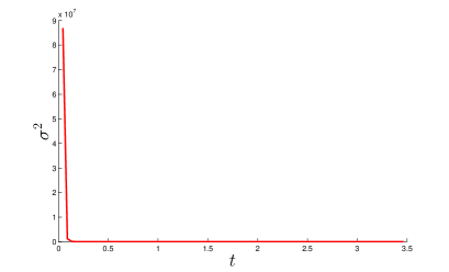
The anisotropy parameter and shear scalar are read as

$$\triangle=\frac{m^{2}(b_{1}^{2}+b_{2}^{2}+b_{3}^{2})}{27\left(\frac{n}{t}+\lambda\right)}[t^{n}exp(\lambda t)]^{-\frac{6}{n}}$$ (20)

$$\sigma^{2}=\frac{(b_{1}^{2}+b_{2}^{2}+b_{3}^{2})}{2}[t^{n}exp(\lambda t)]^{-\frac{6}{n}}$$ (21)

The anisotropy parameter and shear scalar decrease with time that matches with the properties of realistic universe.

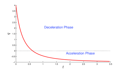
The behaviour of $\rho^{(eff)}$ & $p^{(eff)}$ and deceleration parameter $(q)$ have been graphed in $Figs.~{}1~{}-~{}2$. It is evident that $\rho^{(eff)}$ decreases with time and finally drops to zero for long time and $p^{(eff)}$ is negative throughout the evolution of universe. This behaviour of $\rho^{(eff)}$ and $p^{(eff)}$ match with observed universe. Thus the derived model may able to explain the dynamics of accelerating universe without possible contribution of dark energy/dark matter in $f(R,T)$ gravity. From the right panel of $Fig.~{}1$, one may note that at beginning the DP was positive and universe evolves with deceleration but after some time $q$ becomes negative which have consistency with the model of accelerating universe. At late time the value of $q$ approaches to $-1$ which shows the fastest rate of expansion of universe at late time.

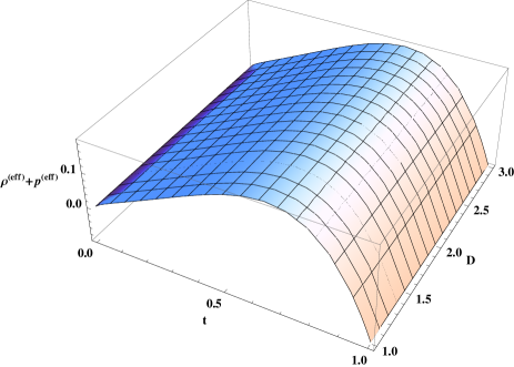
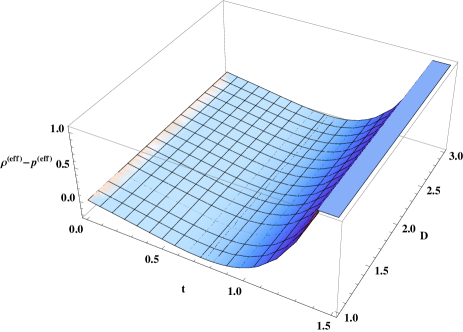
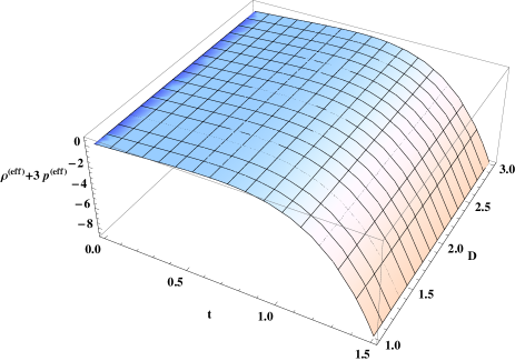
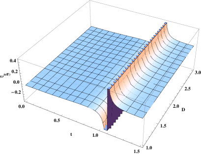
The $\omega^{(eff)}=p^{(eff)}/\rho^{(eff)}$ and single plot of energy conditions have been graphed in $Figs.~{}2-~{}5$. From the left panel of $Fig.~{}2$, it has been noticed that the weak energy condition (WEC) and dominant energy condition (DEC) have been satisfied in the derived model but strong energy condition (SEC) is violated which ensures that anti-gravitational effect - may be one of the possible cause of acceleration. The right panel of $Fig.~{}2$ depicts the behaviour of equation of state parameter $(\omega^{(eff)})$ versus time. For accelerating universe the value of $\omega^{(eff)}$ must be lies in between -1 and 0. In the simplest case, $\omega^{(eff)}=-1$ generates the $\Lambda$CDM model while phantom model and quintessence model also arise when $\omega^{(eff)}<-1$ and $\omega^{(eff)}>-1$ respectively. For our model, we obtain present accepted numerical value of $\omega^{(eff)}$ as $-1$ for longer times.
From equation (13), one may express the scale factor in the term of redshift $(z)$ by taking into account the present value of scale factor i.e. $a_{0}=1$, as following

$$t=\frac{n}{\lambda}W\left[\frac{\lambda}{n}\left(\frac{1}{1+z}\right)\right]^{\frac{m}{n}}$$ (22)

where $W$ denotes the $W$-function or product logarithm.

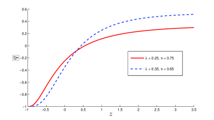
$Fig.~{}6$ depicts the behaviour of DP with redshift for different value of $\lambda$ and $n$. Here we choose the values of constant $\lambda$ and $n$ in agreement with the observational constraints reported in Ozgur/2014 . It is worth to note that the present values of q (i.e. at z = 0) are $-0.25$ and $-0.35$ for $\lambda=0.25$, $n=0.75$ and $\lambda=0.35$, $n=0.65$ respectively. These values are in agreement with recent observational data Hinshaw/2013 . From $Fig.~{}3$, one can check the value of redshift at which the universe transit itself decelerated phase to accelerated expansion. The transition of universe occurs at $z_{tr}=0.55,~{}0.44$ corresponding to the $(\lambda,n)\sim$ $(0.25,0.75)$ and $(0.35,0.75)$ respectively. The WMAP observations Hinshaw/2013 favors the value of $z_{tr}$ obtained for $(\lambda,n)\sim$ $(0.25,0.75)$ that is why we have graphed the other physical parameters by taking $\lambda=0.25$ and $n=0.75$.

V Conclusion

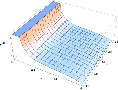
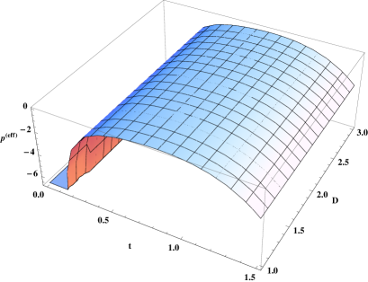
In the present work, we have searched the existence of transitioning scenario of Bianchi-I universe with $f\left(R,T\right)=f_{1}(R)+f_{2}(R)f_{3}(T)$. In particular the exact solution of Einstein’s field equation have been obtained by applying generalized hybrid expansion law of scale factor and functional forms $f_{1}(R)=f_{2}(R)=R$ and $f_{3}(T)=\alpha T$ with $\alpha$ being constant. From left panel of $Fig.~{}1$, one can observe that the effective energy density is positive and decreasing function of time while the effective pressure is negative through out the evolving process of universe. The validation of energy conditions have been graphed in $Figs.~{}3~{}-~{}5$. In the derived model the validation of energy conditions excepts SEC shows that the accelerating universe must violate SEC Barcelo/2002 . The behaviour of anisotropy parameter $(\triangle)$, expansion scalar $(\theta)$, shear scalar $(\sigma^{2})$ and Hubble’s parameters $(H)$ have been graphed in $Fig.~{}7$. The parameters $H$, $\theta$, $\triangle$ and $\sigma^{2}$ start with extremely large values and continue to decrease with passage of time which mimic the present scenario of universe.

It is worth to note that for $m=1$ and $A(t)=B(t)=C(t)=a(t)$, our model reproduces the result obtained in Ref. Moraes/2017 . Thus our model generalizes the solution obtained by Moraes and Sahoo Moraes/2017 and evoke the theory of $f(R,T)$ gravity in anisotropic space-time. Further we analyze that for $\lambda=0$, the dynamics of derived model is governed by power law which gives singular universe with big bang singularity at $t=0$. Similarly for $n=0$, the derived model gives the dynamics of singularity free universe. The DP (q) is found to be positive in early universe and it becomes negative at late time. The present value of $q~{}(z=0)$ is estimated as $-0.25$. This value of DP matches with observational value of q at present epoch, reported in Ref. Hinshaw/2013 . The right panel of $Fig.~{}2$ shows the dynamics of $\omega^{(eff)}$ with passage of time. The evolving range of $\omega^{(eff)}$ in our model is agreed with previous results Yadav/2011 ; Yadav/2011a ; Kumar/2011 ; Saha/2012a .

References

- (1) T. Harko, F.S.N. Lobo, S. Nojiri and S.D. Odintsov, gravity Phys. Rev. D 84 (2011) 024020.
- (2) A. G. Riess et al., Observational Evidence from Supernovae for an Accelerating Universe and a Cosmological Constant Astron. J. 116 (1998) 1009.
- (3) S. Perlmutter et al., Measurements of and from 42 High-Redshift Supernovae Astrophys. J. 517 (1999) 565.
- (4) S. Kumar, R. C. Nunes, Observational constraints on dark matter - dark energy scattering cross section Eur. Phys. J. C. 77 (2017) 734.
- (5) E. Dil, Cosmology of q-deformed dark matter and dark energy Phys. Dark Univ. 16 (2017) 1.
- (6) N. Behrouz et al, Interacting quintom dark energy with Nonminimal Derivative Coupling Phys. Dark Univ. 15 (2017) 72.
- (7) C. Germani, Initial conditions for the Galileon dark energy, Phys. Dark Univ. 15 (2017) 1.
- (8) H. Jennen, J. G. Pereira, Dark energy as a kinematic effect, Phys. Dark Univ. 11 (2016) 49.
- (9) P.H.R.S. Moraes, P.K. Sahoo, The simplest non-minimal matter-geometry coupling in the cosmology Eur. Phys. J. C 77 (2017) 480.
- (10) A.K. Yadav, Bianchi-V string cosmology with power law expansion in gravity Euro Phys. J. Plus 129 (2014) 194.
- (11) A. K. Yadav, A. T. Ali, Invariant Bianchi type I models in gravity Int. J. Geom. Methods in Mod. Phys. doi.org/10.1142/S0219887818500263 (2017)
- (12) A. K. Yadav, P. K. Srivastava, L. Yadav, Hybrid Expansion Law for Dark Energy Dominated Universe in f (R,T) Gravity Int. J. Theor. Phys. 54 (2015) 1671.
- (13) A. K. Yadav, A. Sharma, A transitioning universe with time varying G and decaying Research in Astron. Astrophys. 13, (2013) 501.
- (14) V. Singh, C. P. Singh, Friedmann Cosmology with Matter Creation in Modified Gravity Int. J. Theor. Phys. 55 (2015) 1257.
- (15) L. Parker, Quantized Fields and Particle Creation in Expanding Universes Phys. Rev. D 3 (2071) 2546-2546.
- (16) R. Myrzakulov, FRW Cosmology in gravity Eur. Phys. J. C 72 (2012) 2203.
- (17) M. J. S. Houndjo, Reconstruction of gravity describing matter dominated and accelerated phases Int. J. Mod. Phys. D 21 (2012) 1250003.
- (18) M. Jamil, D. Momeni, M. Raza, R. Mryzakulov, Reconstruction of some cosmological models in cosmology Eur. Phys. J. C 72 (2012) 1999.
- (19) F. Kiani, K. Nozari, Energy conditions in gravity and compatibility with a stable de Sitter solution Phys. Lett. B 728 (2014) 554-561.
- (20) M. Zubair, S. Waheed, Y. Ahmad, Static Spherically Symmetric Wormholes in Gravity Eur. Phys. J. C. 76 (2016) 444.
- (21) Z. Yousaf, M Ilyas, M. Z. Bhatti, Influence of modification of gravity on spherical wormhole models Mod. Phys. Lett. A 32 (2017) 1750163.
- (22) P. H. R. S. Moraes, R. A. C. Correa, R. V. Lobato, Analytical general solutions for static wormholes in gravity JCAP 07 (2017) 029.
- (23) P. H. R. S. Moraes, P.K. Sahoo, Modelling wormholes in gravity Phys. Rev. D 96 (2017) 044038.
- (24) A. Das, F. Rahaman, B. K. Guha, S. Ray, Compact stars in gravity Eur. Phys. J. C 76 (2016) 654
- (25) M. Sharif, Z. Yousaf, Dynamical analysis of self-gravitating stars in gravity Astrophys. Space Sc. 354 (2014) 471.
- (26) H. Shabani, M. Farhoudi, Cosmological and Solar System Consequences of Gravity Models Phys. Rev. D 90 (2014) 044031.
- (27) M. Shen, L. Zhao, Oscillating Quintom Model with Time Periodic Varying Deceleration Parameter Chin. Phys. Lett. 31 (2014) 010401
- (28) O. Akarsu, C. B. Kilinc, LRS Bianchi type I models with anisotropic dark energy and constant deceleration parameter Gen. Relativ. Grav. 42 (2010) 119-140.
- (29) S. Kumar, C. P. Singh, Anisotropic dark energy models with constant deceleration parameter Gen. Relativ. Grav. 43 (2011) 1427-1442.
- (30) A. K. Yadav, B. Saha, LRS Bianchi-I anisotropic cosmological model with dominance of dark energy Astrophys. Space Sc. 337 (2012) 759–765.
- (31) B. Saha, T. Boyadjiev, Bianchi type-I cosmology with scalar and spinor fields Phys. Rev. D 69 (2004) 124010.
- (32) A. K. Yadav, A transitioning universe with anisotropic dark energy Astrophys. Space Sc. 361 (2016) 276.
- (33) C. Barcelo, M. Visser, Twilight for the energy conditions Int. J. Mod. Phys. D 11 (2002) 1553.
- (34) A. Ozgur et al, Cosmology with hybrid expansion law: scalar field reconstruction of cosmic history and observational constraints JCAP 01 (2014) 022
- (35) G. Hinshaw et al, Nine-Year WMAP Observations: Cosmological parameter results Astrophys. J. 208 (2013) 19
- (36) S. Aygun, C. Aktas, I. Yilmaz, Astrophysics & Space Sc. 361 (2016) 380.
- (37) P.H.R.S. Moraes, P.K. Sahoo, G. Ribeiro, R. A. C. Correa, A cosmological scenario from Starobinsky model with formalism arXiv: 1712.07569 [gr-qc] (2017).
- (38) Zaregonbadi R et al, Dark matter from gravity Phys. Rev. D 94 (2016) 084052
- (39) A. K. Yadav, L. Yadav, Bianchi Type III Anisotropic Dark Energy Models with Constant Deceleration Parameter Int. J. Theor. Phys. 50 (2011) 218.
- (40) A. K. Yadav, Some Anisotropic Dark Energy Models in Bianchi Type-V Space-time Astrophys Space Sc. 335 (2011) 565.
- (41) B. Saha, A. K. Yadav, Dark energy model with variable q and in LRS Bianchi-II space-time Astrophys Space Sc. 341 (2012) 651.