Ternary $Z_{2}\times Z_{3}$ graded algebras
and ternary Dirac equation

Abstract

The wave equation generalizing the Dirac operator to the $Z_{3}$-graded case is introduced, whose diagonalization leads to a sixth-order equation. It intertwines not only quark and anti-quark state as well as the $u$ and $d$ quarks, but also the three colors, and is therefore invariant under the product group $Z_{2}\times Z_{2}\times Z_{3}$. The solutions of this equation cannot propagate because their exponents always contain non-oscillating real damping factor. We show how certain cubic products can propagate nevertheless. The model suggests the origin of the color $SU(3)$ symmetry and of the $SU(2)\times U(1)$ that arise automatically in this model, leading to the full bosonic gauge sector of the Standard Model.

1 Introduction

According to the present knowledge, the ultimate undivisible and undestructible constituents of matter, called atoms by ancient Greeks, are in fact the quarks, carrying fractional electric charges and baryonic numbers, two features that appear to be undestructible and conserved under any circumstances.

The notion of Quarks was introduced in elementary particle physics in the early sixties, in now historical papers of M.Gell-Mann, Y.Ne’eman, S.Okubo, A.Zweig ([1], [2], [3]) and others. Since the great success of unitary symmetries in the classification of elementary particles that followed soon later, and since the spectacular development of quantum chromodynamics (QCD), the fact that isolated single quarks can not be observed becomes more mysterious than ever.

Taken into account that quarks evolve inside nucleons as almost point-like entities, one may wonder how the notions of space and time still apply in these conditions ? Perhaps in this case the Lorentz invariance can be derived from some more fundamental discrete symmetries underlying the interactions between quarks ?

If this is the case, then the symmetry $Z_{3}$ must play a fundamental role. The carriers of elementary charges go by packs of three: there are three families of quarks, and three types of leptons.

But the most striking feature is the color charge carried by quarks, and subjected to the exact $SU(3)$ symmetry. The only observable states of quarks are those which mix three colors in equal proportions, giving the so called white, or colorless, combinations. The color symmetry is fundamental in strong interactions, whereas the electroweak interactions ignore the color charge.

In Quantum Chromodynamics quarks are considered as fermions, endowed with spin $\frac{1}{2}$. Only three quarks or anti-quarks can coexist inside a fermionic baryon (respectively, anti-baryon), and a pair quark-antiquark can form a meson with integer spin. Besides, they must belong to different colors, also a three-valued set. There are two quarks in the first generation, $u$ and $d$ (“up” and “down”), which may be considered as two states of a more general object, just like proton and neutron in $SU(2)$ symmetry are two isospin components of a nucleon doublet. In contrast with electrons which cannot occupy the same state with the same spins, but there can be exactly two electrons in the same state with opposite spins, the possibility of coexistence is open for two quarks in the same $u$-state or $d$-state, but not three.

Numerous explanations of the impossibility of observing a pure state of single isolated quark have been proposed. We can cite here the hypothesis that quarks are indeed magnetic monopoles; or that they are confined in ”bags” whose nature was not specified, but whose surface tension was supposed to be too strong to be destroyed by energies actually at our disposal. An attractive potential proportional to the distance between the quarks has been introduced, too, explaining why it is difficult to separate them from each other.

Among these hypotheses, the idea that is at the base of the dual resonance model promoted by J.Scherk [4], supposed that quarks might be just artefacts, somewhat like the poles of a long magnet, being conceived as the ends of an open relativistic string.

It has developed later into an independent new theory of strings and superstrings. This hypothesis seems to be the most radical of all, since it simply rejects the notion of quarks as primary objects, advocating instead the view in which they are perceived as an artefact.

Another brand of thinking is represented by the ideas trying to endow quarks with properties so unusual, that their observability is enhanced by purely algebraic effects: either by mutually annihilating interferences of corresponding wave functions, or some strong statistical effects akin to the Fermi-Dirac statictics that exclude the possibility of observing two identical fermions in the same quantum state at once.

With quarks, one should explain the contrary: namely, why they can be observed only by quark-antiquark pairs, or pure quark or antiquark triplets. Such theories are known as ”algebraic confinement” or ”para-statistics”, using the generalized versions of group theory known under the name of quantum groups acting on quantum spaces whose coordinates do not commute, but satisfy instead more general binary relations of the type $xy=qyx$, $q$ being a complex number [5].

In what follows, we shall investigate the consequences of this type of algebraic confinement hypotheses, stressing the fact that the $Z_{3}$-grading, the ternary algebras and tri-linear forms appear as the most natural and necessary ingredients of these constructions.

2 Fundamental discrete symmetries $Z_{2}$ and $Z_{3}$

As underlined above, the fact that baryons are composed of three quarks displaying three different colors suggests that permutation groups $S_{3}$ and its cyclic group $Z_{3}$ must play an important role in any theory of strong interactions, along with the well established $Z_{2}$ symmetries; the charge conjugation, the space reflection and the time reversal.

The discrete symmetries should act on the Hilbert space of quantum states, which is a linear vector space over the field of complex numbers. Let us briefly recall the elementary properties of complex representations of $S_{3}$ and $Z_{3}$ groups.

We shall denote the primitive third root of unity by $j=e^{2\pi i/3}$. The cyclic abelian subgroup $Z_{3}$ contains three elements corresponding to the three cyclic permutations, which can be represented via multiplication by $j$, $j^{2}$ and $j^{3}=1$ (the identity).

$$\begin{pmatrix}ABC\cr ABC\end{pmatrix}\rightarrow{\bf 1},\,\ \ \,\begin{pmatrix}ABC\cr BCA\end{pmatrix}\rightarrow{\bf j},\,\ \ \,\begin{pmatrix}ABC\cr CAB\end{pmatrix}\rightarrow{\bf j^{2}},$$ (1)

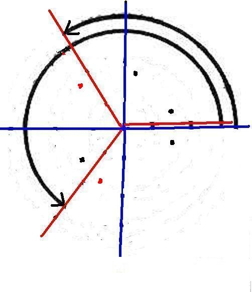
Figure 1: The six $S_{3}$ symmetry transformations are: the identity, two rotations, one by $120^{o}$, another one by $240^{o}$, and three reflections, in the $x$-axis, in the $j$-axis and in the $j^{2}$-axis. The $Z_{3}$ subgroup consists only of the three rotations.

It is important to note that if there are only two distinct states (e.g. $u$ and $d$), the full permutation group $S_{3}$ reduces itself to its abelian subgroup $Z_{3}$, because then even and odd permutations cannot be distinguished, e.g. $uud\rightarrow udu\rightarrow duu$ are the only distinguishable permutations; one needs three different items to make difference between even and odd permutations. The generalization of $Z_{2}$ grading to the $Z_{3}$ grading was proposed in [22], [23].

3 The $Z_{6}$ extension

The presence of color degrees of freedom does not exclude the fundamental $Z_{2}$ symmetry between particles and anti-particles. To take this into account we ought to consider the product group, which will result in the overall $Z_{6}=Z_{2}\times Z_{3}$ symmetry. The cyclic group $Z_{6}$ is represented in the complex plane by all six powers of the non-trivial sixth root of unity, $q=e^{\frac{2\pi i}{6}}.$

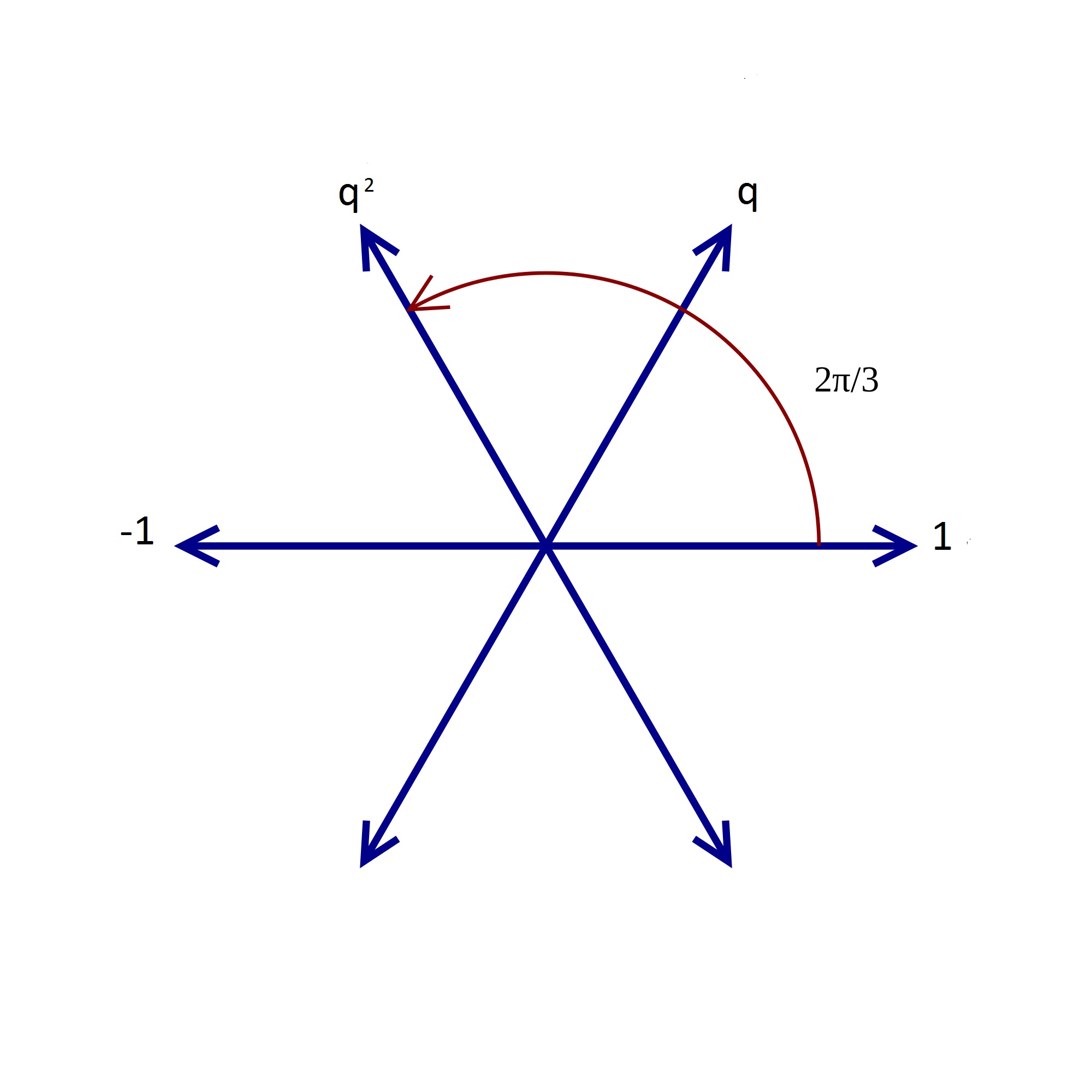
Figure 2: The six complex numbers $q^{k}$ can be put into correrspondence with three colors and three anti-colors.

The superselection rule according to which only observable superpositions of quark states must be ‘white”, or colorless can be implemented by simple algebraic rules of adding roots in $Z_{6}$ (see, e.g. [6]). If we identify zero in the complex plane as corresponding with “white” combination of colors, we get either two “white” combinations of three colors: The three colors: $\;\;q^{2}+q^{4}+q^{6}=j+j^{2}+1=0$. and the three anti-colors:       $q+q^{3}+q^{5}=-j^{2}-1-j=0,$ or the following three “white” combinations of color with its anti-color: $q^{0}$ + $q^{3}$ = $1$ + $(-1)$ = 0,       $q^{2}$ + $q^{5}$ = $j$ + $(-j)$ = 0,       $q^{4}$ + $q$ = $j^{2}$ + $(-j^{2})$ = 0,

These sets of colors should be attributed to three quarks or three anti-quarks, or to the quark-antiquark pairs according to the well known scheme: $uud$ for the proton, $udd$ for the neutron, ${\bar{u}}{\bar{u}}{\bar{d}}$ for the anti-proton and ${\bar{u}}{\bar{d}}{\bar{d}}$ for the anti-neutron. The three pi-mesons are identified with the following quark-antiquark pairs: $u{\bar{d}}$ the $\pi^{+}$, ${\bar{u}}d$ the $\pi^{-}$ and $\frac{1}{\sqrt{2}}(u{\bar{u}}-d{\bar{d}})$ the $\pi^{0}$ meson respectively.

The gluons are the gauge fields that mediate strong interactions between quarks; they provoke color exchange, but in such a way that both initial and final states remain strictly “white”. In the language of second quantization all interactions are composed of creation and annihilation operators: let $B$ symbolize the creation of elementary “blue” charge, and let ${\bar{B}}$ denote the operator of its annihilation (equivalent with creation of its “anti-color”, (yellow in this particular case), etc. Basic interaction consists of replacing of one color by another, e.g. $B{\bar{G}}$ results in replacing green by blue. But such single action performed on a colorless combination will result in two blue charges and one red, which is not “white” anymore. This is why the operator $B{\bar{G}}$ should be always accompanied by its hermitian conjugate $G{\bar{B}}$. This leads to the following set of color interaction carriers:

$$\frac{1}{\sqrt{2}}\;(R{\bar{B}}+B{\bar{R}}),\;\;\;\frac{1}{i\sqrt{2}}(R{\bar{B}}-B{\bar{R}}),\;\;\;\frac{1}{\sqrt{2}}\;(R{\bar{G}}+G{\bar{R}}),$$

$$\frac{1}{i\sqrt{2}}(R{\bar{G}}-G{\bar{R}}),\;\;\;\frac{1}{\sqrt{2}}\;(B{\bar{G}}+G{\bar{B}}),\;\;\;\frac{1}{i\sqrt{2}}(B{\bar{G}}-G{\bar{B}}),$$

$$\frac{1}{\sqrt{2}}\;(R{\bar{R}}-B{\bar{B}}),\;\;\;\frac{1}{\sqrt{6}}(R{\bar{R}}+B{\bar{B}}-2G{\bar{G}}),$$

Acting on a column with three entries, $R,B$ and $G$, these combinations form the basis of eight traceless Gell-Mann $3\times 3$ matrices.

The totally “colorless” quadratic combination does not interact strongly with quarks - it corresponds to the unit matrix, i.e. does not change the color content of the initial configuration. Therefore, the combination

$$R{\bar{R}}+B{\bar{B}}+G{\bar{G}}=0.$$

is not taken into account, so that only eight linear combinations out of nine are independent, forming the basis of the $SU(3)$ algebra generators.

4 Ternary Dirac equation for colors

Before introducing the generalized Dirac equation incorporating the color degrees of freedom, let us remind how the spin degrees of freedom were first introduced by W. Pauli. Historically, as early as in 1925, Pauli arrived at the conclusion that in order to understand electron’s energy levels in atoms, a fourth quantum number is needed, subjected to the exclusion principle, by now bearing Pauli’s name. The identification of this dychotomic quantum number with electron’s spin was made by G. Uhlenbeck and S. Goudsmit, [7] who explored experimentally the anomalous Zeeman effect. In $1927$ Pauli [8] introduced the equation (also bearing his name today) describing the interaction of electron’s spin with external magnetic field. But the way he arrived to this equation and how he missed the relativistic equation for the electron (introduced almost immediately after by P.A.M. Dirac) is very inspiring indeed.

The inclusion of spin variable, subjected to Pauli’s exclusion principle, into a Schroedinger-like equation can be done by replacing the usual complex wave function by a column vector containing two complex components. The energy, momentum and mass operators should be represented by $2\times 2$ matrices. The simplest linear equation considered by Pauli at first had the following form:

$$E\;{\mbox{l1}}_{2}\;\psi=mc^{2}\;{\mbox{l1}}_{2}\;\psi+c\;{\boldsymbol{\sigma}}\cdot{\bf p}\;\psi,$$ (2)

where $\psi$ stays now for the two-component Pauli spinor $\begin{pmatrix}\psi^{1}\cr\psi^{2}\end{pmatrix}$, the $3$-dimensional momentum vector ${\bf p}$ is scalarly multiplied by ${\boldsymbol{\sigma}}$ representing the three hermitian traceless Pauli’s matrices ${\boldsymbol{\sigma}}=[\sigma_{x},\;\sigma_{y},\;\sigma_{z}]$ , and ${\mbox{l1}}_{2}$ stays for the $2\times 2$ unit matrix. But this equation fails to satisfy the Lorentz invariance criterion: it suffices to take the square of the energy operator to discover that (2) leads to the following quadratic relation

$$E^{2}=m^{2}c^{4}+2mc^{3}{\boldsymbol{\sigma}}\cdot{\bf p}+c^{2}\;{\bf p}^{2}$$ (3)

instead of the desired Lorentz-invariant relation $E^{2}=m^{2}c^{4}+c^{2}{\bf p}^{2}$. At this stage the Lorentz invariance could be recovered by introducing another Pauli spinor entangled with the first one via equations similar with (2), but with a negative mass term for the second Pauli spinor:

$$E\;{\mbox{l1}}_{2}\;\psi_{+}=mc^{2}\;{\mbox{l1}}_{2}\;\psi_{+}+c\;{\boldsymbol{\sigma}}\cdot{\bf p}\;\psi_{-},$$

$$E\;{\mbox{l1}}_{2}\;\psi_{-}=-mc^{2}\;{\mbox{l1}}_{2}\;\psi_{-}+c\;{\boldsymbol{\sigma}}\cdot{\bf p}\;\psi_{+},$$ (4)

where $\psi_{+}=\begin{pmatrix}\psi_{+}^{1}\cr\psi_{+}^{2}\end{pmatrix},\;\;\;\psi_{-}=\begin{pmatrix}\psi_{-}^{1}\cr\psi_{-}^{2}\end{pmatrix}$. It is easy to see now that by simple iteration we get the right relation satisfied by simultaneously by both components:

$$E^{2}\psi_{+}-c^{2}{\bf p}^{2}\;\psi_{+}=m^{2}c^{4}\psi_{+},\;\;\;E^{2}\psi_{-}-c^{2}{\bf p}^{2}\;\psi_{-}=m^{2}c^{4}\psi_{-}.$$

The four equations (4) are just one of the representations of the equation of the electron discovered shortly after by Dirac, but in a totally different manner, derived as a “square root” of the Klein-Gordon equation; but at the moment the idea of introducing a negative mass seemed physically unacceptable. This is why Pauli opted for a non-relativistic equation for the electron in the magnetic field,

$$E\;\psi=\left[\frac{1}{2m}({\boldsymbol{\sigma}}\cdot({\bf p}-e{\bf A}))^{2}+eV(x)\right]\psi.=\left[\frac{1}{2m}({\bf p}-e{\bf A})^{2}+e{\boldsymbol{\sigma}}\cdot{\bf B}+eV(x)\right]\psi.$$ (5)

Later on it turned out that the Pauli equation (5) is the non-relativistic limit of the Dirac equation.

The two equations (4) can be re-written using a matrix notation:

$$\begin{pmatrix}E&0\cr 0&E\end{pmatrix}\,\begin{pmatrix}\psi_{+}\cr\psi_{-}\end{pmatrix}=\begin{pmatrix}mc^{2}&0\cr 0&-mc^{2}\end{pmatrix}\,\begin{pmatrix}\psi_{+}\cr\psi_{-}\end{pmatrix}+\begin{pmatrix}0&c\,{\boldsymbol{\sigma}}{\bf p}\cr{\boldsymbol{\sigma}}{\bf p}&0\end{pmatrix}\;\begin{pmatrix}\psi_{+}\cr\psi_{-}\end{pmatrix},$$ (6)

where the entries in the energy operator and the mass matrix are in fact $2\times 2$ identity matrices, as well as the $\sigma$-matrices appearing in the last matrix, so that in reality the above equation represents the $4\times 4$ Dirac equation, only in a different basis [9].

The system of linear equations (6) displays two important discrete $Z_{2}$ symmetries: the space reflection consisting in simultaneous change of the direction of spin and momentum, ${\boldsymbol{\sigma}}\rightarrow-{\boldsymbol{\sigma}},{\bf p}\rightarrow-{\bf p}$, and the particle-antiparticle symmetry realized by the transfromation $m\rightarrow-m,\;\psi_{+}\rightarrow\psi_{-},\;\;\psi_{-}\rightarrow\psi_{+}$. Our next aim is to extend the $Z_{2}\times Z_{2}$ symmetry by including the $Z_{3}$ group which will mix not only the two spin states and particles with anti-particles, but also the three colors.

Now we want to describe three different two-component fields (which can be incidentally given the names of three colors, the “red” one $\varphi_{+}$, the “blue” one $\chi_{+}$, and the “green” one $\psi_{+}$); more explicitly,

$$\varphi_{+}=\begin{pmatrix}\varphi_{+}^{1}\cr\varphi_{+}^{2}\end{pmatrix},\;\chi_{+}=\begin{pmatrix}\chi_{+}^{1}\cr\chi_{+}^{2}\end{pmatrix},\;\psi_{+}=\begin{pmatrix}\psi_{+}^{1}\cr\psi_{+}^{2}\end{pmatrix},$$ (7)

We follow the minimal scheme taking into account the existence of spin by using only Pauli spinors on which the $3$-momentum operator acts through the scalar product ${\boldsymbol{\sigma}}\cdot{\bf p}$. In order to satisfy the required existence of anti-particles, we should also introduce three “anti-colors”, denoted by a “minus” underscript, corresponding to the opposite colors: “cyan” for $\varphi_{-}$, “yellow” for $\chi_{-}$ and “magenta” for $\psi_{-}$; here, too, we have to do with two-component columns:

$$\varphi_{-}=\begin{pmatrix}\varphi_{-}^{1}\cr\varphi_{-}^{2}\end{pmatrix},\;\;\chi_{-}=\begin{pmatrix}\chi_{-}^{1}\cr\chi_{-}^{2}\end{pmatrix},\;\;\psi_{-}=\begin{pmatrix}\psi_{-}^{1}\cr\psi_{-}^{2}\end{pmatrix},$$

all in all twelve components. A somewhat similar construction, but with three Dirac spinors, can be found in [10].

The “colors” should satisfy first order equations conceived in such a way that neither can propagate by itself, just like in the case of ${\bf E}$ and ${\bf B}$ components of Maxwell’s tensor in electrodynamics, or the couple of two-component Pauli spinors which cannot propagate alone, but constitute one single entity, the four-component Dirac spinor.

This leaves little space for the choice of the system of intertwined equations; here is the ternary generalization of Dirac’s equation, intertwining not only particles with antiparticles, but also the three “colors”, in such a way that the entire system becomes invariant under the action of the $Z_{2}\times Z_{2}\times Z_{3}$ group.

The set of linear equations for three Pauli spinors endowed with colors, and another three Pauli spinors corresponding to their anti-particles endowed with ”anti-colors” involves altogether twelve complex functions. The twelve components could describe three independent Dirac particles, but here they will be intertwined in a particular manner, mixing together not only spin states and particle-anti rticle states, but also the three colors.

We shall follow the logic that led from Pauli’s to Dirac’s equation extending it to the colors acted upon by the $Z_{3}$-group. In the expression for the energy operator (i.e. the Hamiltonian), mass terms is positive when acting on particles, and acquires negative sign acting on anti-particles, i.e. it changes sign while intertwining particle-antiparticle components. We shall also assume that the mass term acquires the factor $j$ when we switch from the red component $\varphi$ to the blue component $\xi$, and $j^{2}$ for the green component $\psi$. The momentum operator will be non-diagonal, as in the Dirac equation, systematically intertwining not only particles with antiparticles, but also colors with anti-colors.

The system that satisfies all these assumptions is as follows:

$$E\;\varphi_{+}=mc^{2}\,\varphi_{+}+c\;{\boldsymbol{\sigma}}\cdot{\bf p}\,\chi_{-}$$

$$E\;\chi_{-}=-j\;mc^{2}\,\chi_{-}+c\;{\boldsymbol{\sigma}}\cdot{\bf p}\,\psi_{+}$$

$$E\;\psi_{+}=j^{2}\;mc^{2}\,\psi_{+}+c\;{\boldsymbol{\sigma}}\cdot{\bf p}\,\varphi_{-}$$

$$E\;\varphi_{-}=-mc^{2}\,\varphi_{-}+c\;{\boldsymbol{\sigma}}\cdot{\bf p}\,\chi_{+}$$

$$E\;\chi_{+}=j\;mc^{2}\,\chi_{+}+c\;{\boldsymbol{\sigma}}\cdot{\bf p}\,\psi_{-}$$

$$E\;\psi_{-}=-j^{2}\;mc^{2}\,\varphi_{+}+c\;{\boldsymbol{\sigma}}\cdot{\bf p}\,\varphi_{+}$$ (8)

where

$$\varphi_{+}=\begin{pmatrix}\varphi_{+}^{1}\cr\varphi_{+}^{2}\end{pmatrix},\;\;\varphi_{-}=\begin{pmatrix}\varphi_{-}^{1}\cr\varphi_{-}^{2}\end{pmatrix},\;\;\chi_{+}=\begin{pmatrix}\chi_{+}^{1}\cr\chi_{+}^{2}\end{pmatrix},\;\;\;\chi_{-}=\begin{pmatrix}\chi_{-}^{1}\cr\chi_{-}^{2}\end{pmatrix},\;\;\psi_{+}=\begin{pmatrix}\psi_{+}^{1}\cr\psi_{+}^{2}\end{pmatrix},\;\;\psi_{-}=\begin{pmatrix}\psi_{-}^{1}\cr\psi_{-}^{2}\end{pmatrix},$$

on which Pauli sigma-matrices act in a natural way.

On the right-hand side, the mass terms form a diagonal matrix whose entries follow an ordered row of powers of the sixth root of unity $q=e^{\frac{2\pi i}{6}}$. Indeed, we have

$$m=q^{6}m,\;\;-jm=q^{5}m,\;\;j^{2}m=q^{4}m,$$

$$-m=q^{3}m,\;\;jm=q^{2}m,\;\;-j^{2}m=qm.$$

Let us start the diagonalisation of our system by deriving two third-order equations relating between them the $\varphi_{+}$ and $\varphi_{-}$ fields. By iterating the $E$ operator three times, we get the following equation:

$$E^{3}\;\varphi_{+}=m^{3}c^{6}\;\varphi_{+}-2j\;m^{2}c^{5}\,{\boldsymbol{\sigma}}\cdot{\bf p}\,\chi_{-}-2j\;mc^{3}\,{\boldsymbol{\sigma}}\cdot{\bf p}\,\psi_{+}+\mid{\bf p}\mid^{2}\;{\boldsymbol{\sigma}}\cdot{\bf p}\,\varphi_{-}$$

As one can see, at the third iteration diagonalisation is not yet achieved because of the presence, besides the fields $\varphi_{+}$ and $\varphi_{-}$, of two other fields, namely $\psi_{+}$ and $\chi_{-}$.

Similar third order equations are produced when we start the iteration from any of the five remaining components; in all cases, they contain four terms mixing other components. The diagonalization of the system is achieved only at the sixth iteration.

The final result is extremely simple: all the components satisfy the same sixth-order equation,

$$E^{6}\;\varphi_{+}=m^{6}c^{12}\;\varphi_{+}+c^{6}\mid{\bf p}\mid^{6}\;\varphi_{+},$$

$$E^{6}\;\varphi_{-}=m^{6}c^{12}\;\varphi_{-}+c^{6}\mid{\bf p}\mid^{6}\;\varphi_{-}.$$ (9)

and similarly for all other components.

The energy operator is obviously diagonal, and its action on the spinor-valued column-vector can be represented as a $6\times 6$ operator valued unit matrix. The mass operator is diagonal, too, but its elements represent all powers of the sixth root of unity $q$, which are $q=-j^{2},\;q^{2}=j,\;q^{3}=-1,\;q^{2}=j^{2},\;q^{5}=-j$ and $q^{6}=1$.

Finally, the momentum operator is proportional to a circulant matrix which mixes up all the components of the column vector.

In the basis in which the original system (8) was proposed, the matrix operators can be expressed as follows:

$$M=\begin{pmatrix}m&0&0&0&0&0\cr 0&-m&0&0&0&0\cr 0&0&jm&0&0&0\cr 0&0&0&-jm&0&0\cr 0&0&0&0&j^{2}m&0\cr 0&0&0&0&0&-j^{2}m\end{pmatrix},\;\;\;\;P=\begin{pmatrix}0&0&0&{\boldsymbol{\sigma}}\cdot{\bf p}&0&0\cr 0&0&{\boldsymbol{\sigma}}\cdot{\bf p}&0&0&0\cr 0&0&0&0&0&{\boldsymbol{\sigma}}\cdot{\bf p}\cr 0&0&0&0&{\boldsymbol{\sigma}}\cdot{\bf p}&0\cr 0&{\boldsymbol{\sigma}}\cdot{\bf p}&0&0&0&0\cr{\boldsymbol{\sigma}}\cdot{\bf p}&0&0&0&0&0\end{pmatrix}$$

In fact, the dimension of the two matrices $M$ and $P$ displayed above is $12\times 12$: all the entries in the first one are proportional to the $2\times 2$ identity matrix, so that in the definition one should read

$\begin{pmatrix}m&0\cr 0&m\end{pmatrix}$ instead of $m$, $\begin{pmatrix}jm&0\cr 0&jm\end{pmatrix}$ instead of $j\;m$, etc.

The entries in the second matrix $P$ contain $2\times 2$ Pauli’s sigma-matrices, so that $P$ is also a $12\times 12$ matrix. The energy operator $E$ is proportional to the $12\times 12$ identity matrix.

5 Ternary Clifford Algebra

Using a more rigorous mathematical language the three operators can be expressed in terms of tensor products of matrices of lower dimensions. Let us introduce two following $3\times 3$ matrices:

$$B=\begin{pmatrix}1&0&0\cr 0&j&0\cr 0&0&j^{2}\end{pmatrix}\;\;{\rm and}\;\;Q_{3}=\begin{pmatrix}0&1&0\cr 0&0&1\cr 1&0&0\end{pmatrix}$$ (10)

Then the $12\times 12$ matrices $M$ and $P$ can be represented as the following tensor products:

$$M=m\;B\otimes\sigma_{3}\otimes{\mbox{l1}}_{2},\;\;\;\;P=Q_{3}\otimes\sigma_{1}\otimes({\boldsymbol{\sigma}}\cdot{\bf p})$$ (11)

with as usual, ${\mbox{l1}}_{2},\;\sigma_{1}$ and $\sigma_{3}$ denote the well known $2\times 2$ Pauli’s matrices

$${\mbox{l1}}_{2}=\begin{pmatrix}1&0\cr 0&1\end{pmatrix},\;\;\;\sigma_{1}=\begin{pmatrix}0&1\cr 1&0\end{pmatrix},\;\;\;\sigma_{3}=\begin{pmatrix}1&0\cr 0&-1\end{pmatrix}.$$

The matrices $Q_{a}$ and $Q^{\dagger}_{b}$ span a very interesting ternary algebra. They were considered by Sylvester and Cayley already in the XIX-th century [11]. Out of three independent $Z_{3}$-graded ternary combinations, only one leads to a non-vanishing result. One can check without much effort that both $j$ and $j^{2}$ skew ternary commutators do vanish:

$$\{Q_{1},Q_{2},Q_{3}\}_{j}=Q_{1}Q_{2}Q_{3}+jQ_{2}Q_{3}Q_{1}+j^{2}Q_{3}Q_{1}Q_{2}=0,$$

$$\{Q_{1},Q_{2},Q_{3}\}_{j^{2}}=Q_{1}Q_{2}Q_{3}+j^{2}Q_{2}Q_{3}Q_{1}+jQ_{3}Q_{1}Q_{2}=0,$$

and similarly for the odd permutation, $Q_{2}Q_{1}Q_{3}$.

On the contrary, the totally symmetric combination does not vanish; it is proportional to the $3\times 3$ identity matrix l1:

$$Q_{a}Q_{b}Q_{c}+Q_{b}Q_{c}Q_{a}+Q_{c}Q_{a}Q_{b}=\eta_{abc}\,{\mbox{l1}},\;\;\;a,b,...=1,2,3.$$ (12)

with $\eta_{abc}$ given by the following non-zero components:

$$\eta_{111}=\eta_{222}=\eta_{333}=1,\;\;\;\eta_{123}=\eta_{231}=\eta_{312}=1,$$

$$\eta_{213}=\eta_{321}=\eta_{132}=j^{2}.$$ (13)

all other components vanishing. This relation may serve as the definition of ternary Clifford algebra.

Another set of three matrices is formed by the hermitian conjugates of $Q_{a}$, which coincide, with the squares of corresponding $Q_{a}$’s. It is easy to check that one has

$$Q^{2}_{a}=Q_{a}^{\dagger}$$ (14)

The set of three conjugate matrices $Q^{\dagger}_{a}$ satisfy identities conjugate to (12):

$$Q^{\dagger}_{a}Q^{\dagger}_{b}Q^{\dagger}_{c}+Q^{\dagger}_{b}Q^{\dagger}_{c}Q^{\dagger}_{a}+Q^{\dagger}_{c}Q^{\dagger}_{a}Q^{\dagger}_{b}={\bar{\eta}}_{abc}\,{\mbox{l1}},\;\;\;a,b,...=1,2,3.$$ (15)

with ${\bar{\eta}}_{abc}$ complex conjugate of $\eta_{abc}$.

It is obvious that any similarity transformation of the generators $Q_{a}$ will keep the ternary anti-commutator (13) invariant. As a matter of fact, if we define ${\tilde{Q}}_{b}=P^{-1}Q_{b}P$, with $P$ a non-singular $3\times 3$ matrix, the new set of generators will satisfy the same ternary relations, because

$${\tilde{Q}}_{a}{\tilde{Q}}_{b}{\tilde{Q}}_{c}=P^{-1}Q_{a}PP^{-1}Q_{b}PP^{-1}Q_{c}P=P^{-1}(Q_{a}Q_{b}Q_{c})P,$$

and on the right-hand side we have the unit matrix which commutes with all other matrices, so that $P^{-1}\;{\mbox{l1}}\;P={\mbox{l1}}$.

The six matrices $Q_{a}$ and $Q^{\dagger}_{b},\;\;a,b,...=1,2,3$ are traceless, and one can define six traceless hermitian matrices. forming the following linear combinations: $\frac{1}{2}\;(Q_{a}+Q^{\dagger}_{a})$ and $\frac{1}{2i}\;(Q_{a}-Q^{\dagger}_{a})$.

This is not enough to produce the complete basis for $3$ traceless hermitian matrices, which should be of dimension $8$. Two linearly independent traceless diagonal matrices must be added; we choose the following:

$$B=\begin{pmatrix}1&0&0\cr 0&j&0\cr 0&0&j^{2}\end{pmatrix}\;\;\;\;{\rm and}\;\;\;B^{\dagger}=B^{2}=\begin{pmatrix}1&0&0\cr 0&j^{2}&0\cr 0&0&j\end{pmatrix}.$$ (16)

One can also easily check that

$$B\,B^{\dagger}=B^{\dagger}\,B={\mbox{l1}},\;\;\;\left(B^{\dagger}\right)^{2}=B,\;\;\;\;B^{3}={\bf 1}\;\;\;{\rm and}\left(B^{\dagger}\right)^{3}={\mbox{l1}}.$$ (17)

The set of eight traceless matrices $(Q_{a},Q^{\dagger}_{b},B$ and $B^{\dagger})$ forms an associative algebra over the ring of real numbers tensorized with the groups $Z_{3}$ generated by the complex third root of unity $j=e^{\frac{2\pi i}{3}}$. These matrices can serve as a basis (although unusual) of the $SU(3)$ Lie algebra, see e.g. [12]. The matrices of this type were used recently in the description of Yangians by Yu and Ge ([13]).

The energy operator, proportional to the $12\times 12$ unit matrix, can be written in a similar manner as a product of three unit matrices, ${\mbox{l1}}_{3}\otimes{\mbox{l1}}_{2}\otimes{\mbox{l1}}_{2}$

In the basis in which the functions are aligned in a column by colors, first $\varphi_{+},\chi_{+},\psi_{+}$ followed by $\varphi_{-},\chi_{-},\psi_{-}$, the matrix operators take on another form, namely

$$M=m\;\sigma_{3}\otimes B\otimes{\bf 1}_{2},\;\;\;\;P=\sigma_{1}\otimes Q_{3}\otimes{\boldsymbol{\sigma}}\cdot{\bf p}$$ (18)

Keeping only the mass operator on the right-hand side, we get:

$$E\;\left[{\bf 1}_{2}\otimes{\bf 1}_{3}\otimes{\bf 1}_{2}\right]\;\Psi-c\;\left[\sigma_{1}\otimes Q_{3}\otimes{\boldsymbol{\sigma}}\cdot{\bf p}\right]\;\Psi=mc^{2}\;\left[\sigma_{3}\otimes B\otimes{\bf 1}_{2}\right]\;\Psi$$ (19)

By multiplying on the left by the matrix

$$\sigma_{3}\otimes B^{\dagger}\otimes{\bf 1}_{2}$$

we arrive at the following form of ternary generalization of Dirac’s equation:

$$E\;\left[\sigma_{3}\otimes B^{\dagger}\otimes{\bf 1}_{2}\right]-\left[c\;i\sigma_{2}\otimes j^{2}\,Q_{2}\otimes{\boldsymbol{\sigma}}\cdot{\bf p}\right]\;\Psi=mc^{2}\;{\bf 1}_{2}\otimes{\bf 1_{3}}\otimes{\bf 1}_{2}\;\Psi$$

where we used the fact that under matrix multiplication, $\sigma_{3}\sigma^{3}={\mbox{l1}}_{2}$, $B^{\dagger}B={\mbox{l1}}_{3}$ and $B^{\dagger}Q_{3}=j^{2}\,Q_{2}$.

One can check by direct computation that the sixth power of this operator gives the same result as before,

$$\left[E\;\sigma_{3}\otimes B^{\dagger}\otimes{\mbox{l1}}_{2}-i\sigma_{2}\otimes j^{2}\,Q_{2}\otimes c\,{\boldsymbol{\sigma}}\cdot{\bf p}\right]^{6}=\left[E^{6}-c^{6}{\bf p}^{6}\right]\;{\mbox{l1}}_{12}=m^{6}c^{12}\;{\mbox{l1}}_{12}$$ (20)

The ternary Dirac equation can be written in a concise manner using the Minkowskian indices and the usual pseudo-scalar product of two four-vectors as follows:

$$\Gamma^{\mu}p_{\mu}=mc^{2}\;{\mbox{l1}}_{12}$$ (21)

with $12\times 12$ matrices $\Gamma^{\mu},\mu=0,1,2,3$ defined as follows:

$$\Gamma^{0}=\sigma_{3}\otimes B^{\dagger}\otimes{\mbox{l1}}_{2},\;\;\;\;\hskip 17.07182pt\;\;\;\;\Gamma^{k}=-i\sigma_{2}\otimes j^{2}\,Q_{2}\otimes{\sigma}^{k}$$

6 The $Z_{3}$ Lorentz symmetry

Let us rewrite the matrix operator generating our system when it acts on the column vector containing twelve components of three “color” fields,

$$E\;{\mbox{l1}}_{2}\otimes{\mbox{l1}}_{3}\otimes{\mbox{l1}}_{2}=mc^{2}\;\sigma_{3}\otimes B\otimes{\mbox{l1}}_{2}+\sigma_{1}\otimes Q_{3}\otimes c\,{\boldsymbol{\sigma}}\cdot{\bf p}$$

in a slightly different way, with energy and momentum operators on the left hand side, and the mass operator on the right hand side:

$$E\;{\mbox{l1}}_{2}\otimes{\mbox{l1}}_{3}\otimes{\mbox{l1}}_{2}-\sigma_{1}\otimes Q_{3}\otimes{\boldsymbol{\sigma}}\cdot{\bf p}=mc^{2}\;\sigma_{3}\otimes B\otimes{\mbox{l1}}_{2}$$ (22)

Following a similar procedure applied to the Dirac equation, let us transform this equation so that the mass operator becomes proportional to the unit matrix. Let us multiply this equation from the left by the matrix $\sigma_{3}\otimes B^{\dagger}\otimes{\mbox{l1}}_{2}.$

Now we get the following equation which enable us to interpret the energy and the momentum as the components of a Minkowskian four-vector $c\;p^{\mu}=[E,\;c{\bf p}]$:

$$E\;\sigma_{3}\otimes B^{\dagger}\otimes{\mbox{l1}}_{2}-i\sigma_{2}\otimes j^{2}\,Q_{2}\otimes c\,{\boldsymbol{\sigma}}\cdot{\bf p}=mc^{2}\;{\mbox{l1}}_{2}\otimes{\mbox{l1}}_{3}\otimes{\mbox{l1}}_{2},$$ (23)

where we used the fact that under matrix multiplication, $\sigma_{3}\sigma^{3}={\mbox{l1}}_{2}$, $B^{\dagger}B={\mbox{l1}}_{3}$ and $B^{\dagger}Q_{3}=j^{2}\,Q_{2}$.

One can check by direct computation that the sixth power of this operator gives the same result as before,

$$\left[E\;\sigma_{3}\otimes B^{\dagger}\otimes{\mbox{l1}}_{2}-i\sigma_{2}\otimes j^{2}\,Q_{2}\otimes c\,{\boldsymbol{\sigma}}\cdot{\bf p}\right]^{6}=$$

$$=\left[E^{6}-c^{6}{\bf p}^{6}\right]\;{\mbox{l1}}_{12}=m^{6}c^{12}\;{\mbox{l1}}_{12}$$ (24)

It is also worthwhile to note that not only taking the sixth power of our operator yields the simple algebraic relation (24), but the similar relation exists between the determinants:

$${\rm det}\left(E\;\sigma_{3}\otimes B^{\dagger}\otimes{\mbox{l1}}_{2}-i\sigma_{2}\otimes j^{2}\,Q_{2}\otimes c\,{\boldsymbol{\sigma}}\cdot{\bf p}=\right)=\left(E^{6}-c^{6}\mid{\bf p}\mid^{6}\right)^{2}={\rm det}\left(mc^{2}\;{\mbox{l1}}_{2}\otimes{\mbox{l1}}_{3}\otimes{\mbox{l1}}_{2},\right)=m^{12}c^{24}.$$ (25)

The eigenvalues of the generalized Dirac operator have all the same absolute value $R=\mid(E^{6}-c^{6}\mid{\bf p}\mid^{6})^{\frac{1}{6}}\mid$, and are given by:

$$R,\;-R,\;jR,\;-jR,\;j^{2}R,\;-j^{2}R.$$ (26)

They are double degenerate, i.e. although the characteristic equation is of twelfth order, it has only six distinct eigenvalues. This result will be important for the subsequent discussion of the generalized Lorentz invariance.

Our equation can be written in a concise manner using the Minkowskian indices and the usual pseudo-scalar product of two four-vectors as follows:

$$\Gamma^{\mu}p_{\mu}=mc\;{\mbox{l1}}_{12},\;\;\;{\rm with}\;\;p^{0}=\frac{E}{c},\;\;p^{k}=mc\frac{dx^{k}}{ds}.$$ (27)

with $12\times 12$ matrices $\Gamma^{\mu},\mu=0,1,2,3$ defined as follows:

$$\Gamma^{0}=\sigma_{3}\otimes B^{\dagger}\otimes{\mbox{l1}}_{2},\;\;\;\;\;\;\Gamma^{k}=-i\sigma_{2}\otimes j^{2}\,Q_{2}\otimes{\sigma}^{k}$$ (28)

Unfortunately, the four $12\times 12$ matrices do not satisfy usual anti-commutation relations similar to those of the $4\times 4$ Dirac matrices $\gamma^{\mu}$, i.e. $\gamma^{\mu}\gamma^{\nu}+\gamma^{\nu}\gamma^{\mu}=2\;g^{\mu\nu}\;{\bf 1}_{4}.$

Although the four $12\times 12$ matrices do not satisfy usual anti-commutation relations similar to those of the $4\times 4$ Dirac matrices $\gamma^{\mu}$, i.e. $\gamma^{\mu}\gamma^{\nu}+\gamma^{\nu}\gamma^{\mu}=2\;g^{\mu\nu}\;{\bf 1}_{4}.$ nevertheless, the system of equations satisfied by the 12-dimensional wave function $\Psi$,

$$-i\hbar\;\Gamma^{\mu}\,\partial_{\mu}\,\Psi=mc\Psi$$ (29)

is a hyperbolic one, and has the same light cone as the Klein-Gordon equation. To corroborate this statement, let us first consider the massless case,

$$-i\hbar\;\Gamma^{\mu}\,\partial_{\mu}\,\Psi=0.$$ (30)

Assuming the general solution of the form $e^{k_{\mu}x^{\mu}}$, we can replace the derivations by the components of the wave 4-vector $k^{\mu}$, and take the sixth power of the matrix $\Gamma^{\mu}k_{\mu}$. The resulting dispersion relation was shown to be

$$k_{0}^{6}-\mid{\bf k}\mid^{6}=\left(k_{0}^{2}-\mid{\bf k}\mid^{2}\right)\left(k_{0}^{2}-j\;\mid{\bf k}\mid^{2}\right)\left(k_{0}^{2}-j^{2}\;\mid{\bf k}\mid^{2}\right)=$$

$$=\left(k_{0}^{2}-\mid{\bf k}\mid^{2}\right)\;\left(k_{0}^{4}+k_{0}^{2}\mid{\bf k}\mid^{2}+\mid{\bf k}\mid^{4}\right)=0.$$

The first factor defines the usual light cone, while the factor of degree four is strictly positive (besides the origin $0$). The system has only one characteristic surface which is the same for all massless fields. Each of the three factors remains invariant under a different representation of the $SL(2,{\bf C})$ group.

Let us introduce the following three matrices representing the same four-vector $k^{\mu}$:

$$K_{3}=\begin{pmatrix}k_{0}&k_{x}\cr k_{x}&k_{0}\end{pmatrix},\;\;K_{1}=\begin{pmatrix}k_{0}&jk_{x}\cr jk_{x}&k_{0}\end{pmatrix},\;\;K_{2}=\begin{pmatrix}k_{0}&j^{2}k_{x}\cr j^{2}k_{x}&k_{0}\end{pmatrix},$$ (31)

whose determinants are, respectively,

$${\rm det}K_{1}=k_{0}^{2}-j^{2}k_{x}^{2},\;\;\;{\rm det}K_{2}=k_{0}^{2}-jk_{x}^{2},\;\;{\rm det}K_{3}=k_{0}^{2}-k_{x}^{2}.$$ (32)

Note that only the third matrix $K_{3}$ is hermitian, and corresponds to a real space-time vector $k^{\mu}$, while neither of the remaining two matrices $K_{1}$ and $K_{2}$ is hermitian; however, one is the hermitian conjugate of another.

In what follows, we shall replace the absolute value of the wave vector $\mid{\bf k}\mid$ by a single spatial component, say $k_{x}$, because for any given $4$-vector $k^{\mu}=[k_{0},{\bf k}]$ we can choose the coordinate system in such a way that its $x$-axis should be aligned along the vector ${\bf k}$. Then it is easy to check that one has:

$$\begin{pmatrix}\cosh u&\sinh u\cr\sinh u&\cosh u\end{pmatrix}\begin{pmatrix}k_{0}\cr k_{x}\end{pmatrix}=\begin{pmatrix}{k^{\prime}}_{0}\cr{k^{\prime}}_{x}\end{pmatrix}$$

$$\begin{pmatrix}\cosh u&j^{2}\sinh u\cr j\sinh u&\cosh u\end{pmatrix}\begin{pmatrix}k_{0}\cr j\;k_{x}\end{pmatrix}=\begin{pmatrix}{k^{\prime}}_{0}\cr j\;{k^{\prime}}_{x}\end{pmatrix}$$

$$\begin{pmatrix}\cosh u&j\sinh u\cr j^{2}\sinh u&\cosh u\end{pmatrix}\begin{pmatrix}k_{0}\cr j^{2}k_{x}\end{pmatrix}=\begin{pmatrix}{k^{\prime}}_{0}\cr j^{2}{k^{\prime}}_{x}\end{pmatrix}$$ (33)

The transformed vectors are given by the following expressions:

$$\hskip 14.22636pti)\;\;k^{{}^{\prime}}_{0}=k_{0}\cosh u+k_{x}\;\sinh u,\;\;\;k^{{}^{\prime}}_{x}=k_{0}\sinh u+k_{x}\;\cosh u$$

$$\hskip 8.5359ptii)\;\;k^{{}^{\prime}}_{0}=k_{0}\cosh u+j^{2}\;k_{x}\;\sinh u,\;\;\;k^{{}^{\prime}}_{x}=j\;k_{0}\sinh u+k_{x}\;\cosh u$$

$$iii)\;\;k^{{}^{\prime}}_{0}=k_{0}\cosh u+j\;k_{x}\;\sinh u,\;\;\;k_{x}^{{}^{\prime}}=j^{2}\;k_{0}\sinh u+k_{x}\;\cosh u$$

Let us now introduce a $6\times 6$ matrix composed out of the above three $2\times 2$ matrices:

$$\begin{pmatrix}0&k_{0}\;{\mbox{l1}}_{2}+{\bf k}\cdot{\boldsymbol{\sigma}}&0\cr 0&0&k_{0}\;{\mbox{l1}}_{2}+j\,{\bf k}\cdot{\boldsymbol{\sigma}}\cr k_{0}\;{\mbox{l1}}_{2}+j^{2}\,{\bf k}\cdot{\boldsymbol{\sigma}}&0&0\end{pmatrix}$$ (34)

or, more explicitly,

$${\Large K}=\begin{pmatrix}0&0&k_{0}&k_{x}&0&0\cr 0&0&k_{x}&k_{0}&0&0\cr 0&0&0&0&k_{0}&jk_{x}\cr 0&0&0&0&jk_{x}&k_{0}\cr k_{0}&j^{2}k_{x}&0&0&0&0\cr j^{2}k_{x}&k_{0}&0&0&0&0\end{pmatrix}$$ (35)

It is easy to check that

$${\rm det\Large K}=\left({\rm det}K_{1}\right)\cdot\left({\rm det}K_{2}\right)\cdot\left({\rm det}K_{3}\right)$$

$$=(k_{0}^{2}-k_{x}^{2})(k_{0}^{2}-j^{2}k_{x}^{2})(k_{0}^{2}-jk_{x}^{2})=k_{0}^{6}-k_{x}^{6}.$$ (36)

It is also remarkable that the determinant remains the same in the basis in which the ternary Dirac operator was proposed, namely when we consider the matrix

$${\Large K}=\begin{pmatrix}k_{0}&0&0&k_{x}&0&0\cr 0&k_{0}&k_{x}&0&0&0\cr 0&0&k_{0}&0&0&jk_{x}\cr 0&0&0&k_{0}&jk_{x}&0\cr 0&j^{2}k_{x}&0&0&k_{0}&0\cr j^{2}k_{x}&0&0&0&0&k_{0}\end{pmatrix}$$ (37)

Let us show now that the spinorial representation of Lorentz boosts can be applied to each of the three matrices $K_{1},K_{2}$ and $K_{3}$ separately, keeping their determinants unchanged. As a matter of fact, besides the well-known formula:

$$\begin{pmatrix}\cosh\frac{u}{2}&\sinh\frac{u}{2}\cr\sinh\frac{u}{2}&\cosh\frac{u}{2}\end{pmatrix}\hskip 5.69046pt\begin{pmatrix}k_{0}&k_{x}\cr k_{x}&k_{0}\end{pmatrix}\hskip 5.69046pt\begin{pmatrix}\cosh\frac{u}{2}&\sinh\frac{u}{2}\cr\sinh\frac{u}{2}&\cosh\frac{u}{2}\end{pmatrix}=\begin{pmatrix}{k^{\prime}}_{0}&{k^{\prime}}_{x}\cr{k^{\prime}}_{x}&{k^{\prime}}_{0}\end{pmatrix},$$ (38)

with

$${k^{\prime}}_{0}=k_{0}\;\cosh u+k_{x}\;\sinh u,\;\;\;\;{k^{\prime}}_{x}=k_{0}\;\sinh u+k_{x}\;\cosh u.$$ (39)

which becomes apparent when we remind that

$$\cosh^{2}\frac{u}{2}+\sinh^{2}\frac{u}{2}=\cosh u\;\;{\rm and}\;\;2\sinh\frac{u}{2}\;\cosh\frac{u}{2}=\sinh u,$$

keeping unchanged the Minkowskian scalar product: ${k^{\prime}}^{2}_{0}-{k^{\prime}}_{x}^{2}=k_{0}^{2}-k_{x}^{2}$, we have also two transformations of the same kind which keep invariant the “complexified” Minkowskian squares appearing as factors in the sixth-orer expression $k_{0}^{6}-k_{x}^{6}$, namely

$$k_{0}^{2}-j\;k_{x}^{2}\;\;\;\;{\rm and}\;\;\;k_{0}^{2}-j^{2}\;k_{x}^{2}.$$

The above expressions can be identified as the determinants of the following $2\times 2$ matrices:

$$k_{0}^{2}-j\;k_{x}^{2}={\rm det}\begin{pmatrix}k_{0}&j^{2}k_{x}^{2}\cr j^{2}\;k_{x}&k_{0}\end{pmatrix},\;\;\;\;k_{0}^{2}-j^{2}\;k_{x}^{2}={\rm det}\begin{pmatrix}k_{0}&jk_{x}^{2}\cr j\;k_{x}&k_{0}\end{pmatrix}.$$ (40)

It is easy to check that we have:

$$\begin{pmatrix}\cosh\frac{u}{2}&\sinh\frac{u}{2}\cr\sinh\frac{u}{2}&\cosh\frac{u}{2}\end{pmatrix}\begin{pmatrix}k_{0}&jk_{x}\cr jk_{x}&k_{0}\end{pmatrix}\begin{pmatrix}\cosh\frac{u}{2}&\sinh\frac{u}{2}\cr\sinh\frac{u}{2}&\cosh\frac{u}{2}\end{pmatrix}=\begin{pmatrix}{k^{\prime}}_{0}&j{k^{\prime}}_{x}\cr j{k^{\prime}}_{x}&{k^{\prime}}_{0}\end{pmatrix},$$ (41)

with ${k^{\prime}}_{0}=k_{0}\;\cosh u+j\;{k^{\prime}}_{x}\;\sinh u$, so that ${k^{\prime}}_{0}^{2}-j{k^{\prime}}_{x}^{2}=k_{0}^{2}-jk_{x}^{2}$, as well as

$$\begin{pmatrix}\cosh\frac{u}{2}&\sinh\frac{u}{2}\cr\sinh\frac{u}{2}&\cosh\frac{u}{2}\end{pmatrix}\begin{pmatrix}k_{0}&j^{2}\;k_{x}\cr j^{2}\;k_{x}&k_{0}\end{pmatrix}\begin{pmatrix}\cosh\frac{u}{2}&\sinh\frac{u}{2}\cr\sinh\frac{u}{2}&\cosh\frac{u}{2}\end{pmatrix}=\begin{pmatrix}{k^{\prime}}_{0}&j^{2}{k^{\prime}}_{x}\cr j^{2}{k^{\prime}}_{x}&{k^{\prime}}_{0}\end{pmatrix},$$ (42)

The bottom line is the following: the $12\times 12$ matrix formed by the tensor product of $\sigma_{3}$ with the $6\times 6$ matrix $K$ defined above, has the same determinant and the same eigenvalues (25, 26) as the generalized Dirac operator 22, if we replace $k_{0}$ by $E$ and ${\bf k}$ by $c{\bf p}$. We have shown that the determinant of the matrix $\sigma_{3}\otimes K$ (equal to $(k_{0}^{6}-k_{x}^{6})^{2}$ remains invariant under the generalized Lorentz transformation composed of three representations, the usual unitary one and two complex ones. Therefore there exists a similarity between the two matrices, which preserves the invariance under the generalized Lorentz group intertwined with $Z_{3}$.

7 Interaction with gauge fields

The matrix representation of the system (22) is by no means unique. In the form which most closely resembles the classical Dirac equation, we chose the following representation for our ternary Dirac operator (designed be ${\cal{D}}$ for convenience):

$${\cal{D}}=E\;\sigma_{3}\otimes B^{\dagger}\otimes{\mbox{l1}}_{2}-(i\sigma_{2}\otimes jQ_{2}\otimes c\;{\boldsymbol{\sigma}}\cdot{\bf p}=mc^{2}\;{\mbox{l1}}_{2}\otimes{\mbox{l1}}_{3}\otimes{\mbox{l1}}_{2}$$ (43)

Obviously, the essential sixth order diagonalized system resulting from the sixth iteration of this operator, as well as its characteristic equation and eigenvalues remain unchanged under an arbitrary similarity transformation, ${\cal{D}}\rightarrow P^{-1}{\cal{D}}P$. Taking into account the particular tensorial structure of ternary Dirac operator, the matrices $P$ should display similar structure in order to keep the three factors separated. This reduces the allowed similarity matrices to the following family:

$$P=R\otimes S\otimes U,\;\;$$

with $R$ being a $2\times 2$ matrix, $S$ denoting a $3\times 3$ matrix, and $U$ proportional to the $2\times 2$ unit matrix in order not to change the scalar product ${\boldsymbol{\sigma}}\cdot{\bf p}$ in the last tensorial factor in ${\cal{D}}$.

The minimal coupling between the Dirac particles (electrons and positrons) with the electromagnetic field is obtained by inserting the four-potential $A_{\mu}$ into the Dirac equation:

$$\gamma^{\mu}(p_{\mu}-e\;A_{\mu})\;\psi=m\;\psi.$$ (44)

Ternary generalization of Dirac’s equation, when expressed with explicit Minkowskian indices, offers a similar possibility of introducing gauge fields. The particular structure of $12\times 12$ matrices $\Gamma_{\mu}$ makes possible the accomodation of three types of gauge fields, corresponding to three factors from which the tensor product results.

The overall gauge field can be decomposed into a sum of three contributions: the $SU(3)$ gauge field $\lambda_{a}B^{a}_{\mu}$, with $\lambda_{a},\;\;\;a=1,2,..8$ denoting the eight $3\times 3$ traceless Gell-Mann matrices, the $SU(2)$ gauge field $\sigma_{k}\,A^{k}_{\mu},\;\;\;k=1,2,3$ and the electric field potential $A_{\mu}$. We propose to insert each of these gauge potentials into a common $12\times 12$ matrix as follows: The strong interaction gauge potential is aligned on the $SU(3)$ matrix basis:

$$B_{\mu}={\mbox{l1}}_{2}\otimes{\lambda}_{a}B^{a}_{\mu}\otimes{\mbox{l1}}_{2},\;\;,a,b=1,2,...8.$$

appearing as the second factor in the tensor product;

The $SU(2)$ weak interaction potential $A^{i}_{\mu}$ aligned along the three $\sigma$-matrices of the first tensorial factor

$$\sigma_{k}\,A^{k}_{\mu}\otimes{\mbox{l1}}_{3},\;\;\;i,k,..=1,2,3.$$

and the electromagnetic potential $A^{em}_{\mu}$ aligned along the unit $2\times 2$ matrix appearing as the third factor in the tensor product.

$$\otimes A_{\mu}\,{\mbox{l1}}_{2}$$

so that the overall expression for the gauge potential becomes:

$${\cal{A}}_{\mu}={\mbox{l1}}_{2}\otimes{\lambda}_{a}B^{a}_{\mu}\otimes{\mbox{l1}}_{2}+\sigma_{k}\,A^{k}_{\mu}\otimes{\mbox{l1}}_{3}\otimes{\mbox{l1}}_{2}+{\mbox{l1}}_{2}\otimes{\mbox{l1}}_{3}\otimes A^{em}_{\mu}\,{\mbox{l1}}_{2}$$ (45)

The proposed ternary generalization of Dirac’s equation including color degrees of freedom contains naturally not only the $SU(3)$-invariant strong interactions, but leads automatically to another type of gauge fields to which quarks are also sensitive: these are the gauge fields generated by the $SU(2)$ and $U(1)$ symmetries incorporated in the system.

There is an extra bonus here: namely, one can look at the same system (22) in the limit when the color interaction is switched off. This amounts to replacing the $3\times 3$ matrices $B$ and $Q_{3}$ by unit matrices ${\mbox{l1}}_{3}.$ The resulting system is equivalent with a cartesian product of three identical Dirac equations:

$$E\;{\mbox{l1}}_{2}\otimes{\mbox{l1}}_{3}\otimes{\mbox{l1}}_{2}-\sigma_{1}\otimes{\mbox{l1}}_{3}\otimes{\boldsymbol{\sigma}}\cdot{\bf p}=mc^{2}\;\sigma_{3}\otimes{\mbox{l1}}_{3}\otimes{\mbox{l1}}_{2}$$ (46)

Without any symmetry breaking, this set of equations describes three identical fermions sensitive exclusively to the $SU(2)\times U(1)$ gauge fields, i.e. the electroweak interaction, like the elementary particles known as leptons - in this setting they appear as natural colorless companions of quarks. This sheds new light on the fact that their number is equal, and even if other families of quarks had to be introduced (which we did not consider here), described by a similar ternary Dirac system, they would also give rise to another set of three leptons. And this is what the experimental data confirmed since the discovery of the families with other “flavors”. The gauge fields are obviously common to all families.

In principle, we should have started with zero masses for all particles, quarks and leptons alike, and let the Higgs-Kibble mechanism generate non-zero masses. The Higgs field necessary for this to happen can be introduced like in the model of matrix algebras in the context of non-commutative geometry, (see [14], [15], [16]; see also [17]).

8 Solutions

The system of twelve linear equations supposed to describe the dynamics of three intertwined fields was shown to be represented by a single matrix operator acting on a $12$-component vector: symbolically $E\Psi=(c^{2}M+cP)\Psi.$ By consecutive application of this matrix operator we are able separate the variables and find the common equation of sixth order that is satisfied by each of the components:

$$E^{6}\Psi=m^{6}c^{12}\Psi+c^{6}\,{\bf p}^{6}\Psi.$$ (47)

Applying the quantum correspondence principle, the above equation relating mass, energy and momentum (47) is transformed into a linear differential equation of the sixth order. Indeed, according to

$$E\rightarrow-i\,\hbar\frac{\partial}{\partial t},\;\;\;\;{\bf p}\rightarrow-i\,\hbar\,{\boldsymbol{\nabla}},$$ (48)

we get the following sixth-order partial differential equation to be satisfied by all the components of the wave function $\Psi$.

$$-{\hbar}^{6}\frac{\partial^{6}}{\partial t^{6}}\psi-m^{6}c^{12}\psi=-{\hbar}^{6}{\Delta}^{3}\psi.$$ (49)

Identifying quantum operators of energy and momentum,

$$-i{\hbar}\frac{\partial}{\partial t}\rightarrow E,\;\;\;-i{\hbar}{\bf\nabla}\rightarrow{\bf p},$$

Let us write the algebraic expression relating mass, energy and momentum (47) simply as follows:

$$E^{6}-m^{6}c^{12}=\mid{\bf p}\mid^{6}c^{6}.$$ (50)

This equation can be factorized showing how it was obtained by subsequent action of the operators of the system of six equations:

$$E^{6}-m^{6}c^{12}=(E^{3}-m^{3}c^{6})(E^{3}+m^{3}c^{6})=$$

$$(E-mc^{2})(jE-mc^{2})(j^{2}E-mc^{2})(E+mc^{2})(jE+mc^{2})(j^{2}E+mc^{2})=\mid{\bf p}\mid^{6}c^{6}.$$

This sixth-order equation can be solved by separation of variables; the time-dependent and the space-dependent factors have the same structure:

$$A_{1}\,e^{\omega\,t}+A_{2}\,e^{j\,\omega\,t}+A_{3}e^{j^{2}\,\omega\,t},\,\ \ \ \ B_{1}\,e^{{\bf k.r}}+B_{2}\,e^{j\,{\bf k.r}}+B_{3}\,e^{j^{2}\,{\bf k.r}}$$

with $\omega$ and ${\bf k}$ satisfying the following dispersion relation:

$$\frac{\omega^{6}}{c^{6}}+\frac{m^{6}c^{6}}{{\hbar}^{6}}=\mid{\bf k}\mid^{6},$$ (51)

where we have identified $E={\hbar\omega}$ and ${\bf p}={\hbar}{\bf k}$.

Up to this point we follow exactly the way in which the Klein-Gordon equation is deduced from the Dirac equation as the common condition to be satisfied by all the components of the Dirac spinor:

$$E^{2}\psi=m^{2}c^{4}\psi+c^{2}{\bf p}^{2}\psi\;\;\rightarrow\;\;-\hbar^{2}\frac{\partial^{2}\psi}{\partial t^{2}}=m^{2}c^{4}\psi-\hbar^{2}\triangle\psi.$$ (52)

The solutions are saught in the plane wave form $\psi\sim e^{i(\omega t+{\bf k}\cdot{\bf r})}$. Due to the purely imaginary exponential, after such a substitution the Klein-Gordon equation reduces to the well known algebraic condition

$$\hbar^{2}\omega^{2}=m^{2}c^{4}+\hbar^{2}{\bf k}^{2},$$ (53)

which coincides with the previously established relation between the energy, momentum and mass due to the correspondence $E=\hbar\omega$ and ${\bf p}=\hbar{\bf k}$ introduced by de Broglie.

The sixth-order dispersion relation is invariant under the action of $Z_{2}\times Z_{3}=Z_{6}$ symmetry, because to any solution with given real $\omega$ and ${\bf k}$ one can add solutions with $\omega$ replaced by $j\omega$ or $j^{2}\omega$, $j{\bf k}$ or $j^{2}{\bf k}$, as well as $-\omega$; there is no need to introduce also $-{\bf k}$ instead of ${\bf k}$ because the vector ${\bf k}$ can take on all possible directions covering the unit sphere.

The nine complex solutions with positive frequency $\omega$ as well as with $j\;\omega$ and $j^{2}\;\omega$ obtained by the action of the $Z_{3}$-group can be displayed in a compact manner in form of a $3\times 3$ matrix. The inclusion of the essential $Z_{2}$-symmetry ensuring the existence of anti-particles leads to the nine similar solutions with negative $\omega$. The two matrices are displayed below:

$$\begin{pmatrix}e^{\omega\,t+{\bf k\cdot r}}&e^{\omega\,t+j{\bf k\cdot r}}&e^{\omega\,t+j^{2}{\bf k\cdot r}}\cr e^{j\omega\,t+{\bf k\cdot r}}&e^{j\omega\,t+j{\bf k\cdot r}}&e^{j\omega\,t+j^{2}{\bf k\cdot r}}\cr e^{j^{2}\omega\,t+{\bf k\cdot r}}&e^{j^{2}\omega\,t+{\bf k\cdot r}}&e^{j^{2}\omega\,t+j^{2}{\bf k\cdot r}}\end{pmatrix},\;\;\;\;\;\begin{pmatrix}e^{-\omega\,t-{\bf k\cdot r}}&e^{-\omega\,t-j{\bf k\cdot r}}&e^{-\omega\,t-j^{2}{\bf k\cdot r}}\cr e^{-j\omega\,t-{\bf k\cdot r}}&e^{-j\omega\,t-j{\bf k\cdot r}}&e^{-j\omega\,t-j^{2}{\bf k\cdot r}}\cr e^{-j^{2}\omega\,t-{\bf k\cdot r}}&e^{-j^{2}\omega\,t-{\bf k\cdot r}}&e^{-j^{2}\omega\,t-j^{2}{\bf k\cdot r}}\end{pmatrix}$$

and their nine real linear combinations can be represented in the following $3\times 3$ matrix of functions as follows:

$$\begin{pmatrix}e^{\omega\,t+{\bf k\cdot r}}&e^{\omega\,t-\frac{{\bf k\cdot r}}{2}}\,\cos({\bf K}\cdot{\bf r})&e^{\omega\,t-\frac{{\bf k\cdot r}}{2}}\,\sin({\bf K}\cdot{\bf r})\cr e^{-\frac{\omega\,t}{2}+{\bf k\cdot r}}\,\cos\Omega\,t&e^{-\frac{\omega\,t}{2}-\frac{\bf k\cdot r}{2}}\,\cos(\Omega\,t-{\bf K}\cdot{\bf r})&e^{-\frac{\omega\,t}{2}-\frac{{\bf k\cdot r}}{2}}\,\cos(\Omega\,t-{\bf K}\cdot{\bf r})\cr e^{-\frac{\omega\,t}{2}+{\bf k\cdot r}}\,\sin\Omega\,t&e^{-\frac{\omega\,t}{2}-\frac{{\bf k\cdot r}}{2}}\,\sin(\Omega\,t-{\bf K}\cdot{\bf r})&e^{-\frac{\omega\,t}{2}-\frac{{\bf k\cdot r}}{2}}\,\sin(\Omega\,t-{\bf K}\cdot{\bf r})\end{pmatrix},$$

where $\Omega=\frac{\sqrt{3}}{2}\,\omega$ and ${\bf K}=\frac{\sqrt{3}}{2}{\bf k}$; the same can be done with the conjugate solutions (with $-\omega$ instead of $\omega$). A similar matrix, of course, can be produced for the alternative negative $\omega$ choice.

The functions displayed in the matrix do not represent a wave; however, one can produce a propagating solution by forming certain cubic combinations, e.g.

$$e^{\omega\,t+{\bf k\cdot r}}\,e^{-\frac{\omega\,t}{2}-\frac{{\bf k\cdot r}}{2}}\,\cos(\Omega\,t-{\bf K}\cdot{\bf r})\,e^{-\frac{\omega\,t}{2}-\frac{{\bf k\cdot r}}{2}}\,\sin(\Omega\,t-{\bf K}\cdot{\bf r})=\frac{1}{2}\,\sin(2\Omega\,t-2{\bf K}\cdot{\bf r}).$$

What we need now is a multiplication scheme that would define triple products of non-propagating solutions yielding propagating ones, like in the example given above, but under the condition that the factors belong to three distinct subsets (which can be later on identified as “colors”).

Before we proceed farther, let us remind that the set of six independent functions is expected to generate the most general solution of our sixth-order differential equation. Therefore, among the nine functions displayed in the above matrices, as well as in the real basis, three are superfluous. Indeed, the determinants of the two complex matrices of solutions, as well as that of the real matrix, identically vanish. Their lower $2\times 2$ minors are also zero, which confirms the idea that only six out of nine functions are independent. In principle, we could pick up any six functions, but for symmetry reasons we shall remove the diagonal ones. The remaining six functions are displayed in the truncated matrix:

$$\begin{pmatrix}0&e^{\omega\,t-\frac{{\bf k\cdot r}}{2}}\,\cos({\bf K}\cdot{\bf r})&e^{\omega\,t-\frac{{\bf k\cdot r}}{2}}\,\sin({\bf K}\cdot{\bf r})\cr e^{-\frac{\omega\,t}{2}+{\bf k\cdot r}}\,\cos\Omega\,t&0&e^{-\frac{\omega\,t}{2}-\frac{{\bf k\cdot r}}{2}}\,\cos\;u\cr e^{-\frac{\omega\,t}{2}+{\bf k\cdot r}}\,\sin\Omega\,t&e^{-\frac{\omega\,t}{2}-\frac{{\bf k\cdot r}}{2}}\,\sin\;u&0\end{pmatrix},$$

where $u=\Omega\,t-{\bf K}\cdot{\bf r}$.

In what follows, we shall choose the Cartesian system of space coordinates with its $x$-axis aligned with the vector ${\bf k}$, so that in all the six remaining functions displayed in the real matrix we can replace the scalar product ${\bf k}\cdot{\bf r}$ by $kx$, and ${\bf K}\cdot{\bf r}$ by $Kx$, with $K=\frac{\sqrt{3}}{2}\,k$.

With this in mind, let us display the six independent solutions in the following two groups of three:

$$F_{1}=e^{-\frac{\omega t}{2}+kx}\;\sin\Omega t,\;\;\;\;\;\;\;F_{2}=e^{-\frac{\omega t}{2}+kx}\;\cos\Omega t,$$

$$G_{1}=e^{\omega t-\frac{kx}{2}}\;\sin Kx,\;\;\;\;\;\;\;G_{2}=e^{\omega t-\frac{kx}{2}}\;\cos Kx,$$

$$H_{1}=e^{-\frac{\omega t}{2}-\frac{kx}{2}}\;\sin(\Omega t-Kx),\;\;\;\;\;H_{2}=e^{-\frac{\omega t}{2}-\frac{kx}{2}}\;\cos(\Omega t-Kx).$$ (54)

Neither of the six functions above can represent a freely propagating wave: even the last two functions, $H_{1}$ and $H_{2}$ contain, besides the running sinusoidal waves, the real exponentials which have a damping effect. (The wave cannot penetrate distances greater than a few wavelengths, and can last only for times comparable with few oscillations).

However, we shall show that certain cubic expressions can represent a freely propagating wave, without any damping factors. Taking a closer look at the six solutions displayed above, we see that the only way to get rid of the real exponents present in all those functions, but different damping factors, is to form cubic expressions constructed with three functions labelled with three different letters.

Here is the exhaustive list of eight admissible cubic combinations:

$$F_{1}\;G_{1}\;H_{1},\;\;\;F_{2}\;G_{1}\;H_{1};\;\;\;F_{1}\;G_{1}\;H_{2},\;\;\;F_{2}\;G_{1}\;H_{2};$$

$$F_{1}\;G_{2}\;H_{1},\;\;\;F_{2}\;G_{2}\;H_{1};\;\;\;F_{1}\;G_{2}\;H_{2},\;\;\;F_{2}\;G_{2}\;H_{2};$$

But these expressions still contain, besides running waves with double frequency $2\Omega$, undesirable functions like $\sin\Omega t$ or $\cos Kx$. To take an example, we have

$$F_{1}\,G_{2}\,H_{2}=\sin\Omega t\;\cos Kx\;\cos(\Omega t-Kx)=$$

$$\frac{1}{2}\;\left[\sin(\Omega t+Kx)+\sin(\Omega t-Kx)\right]\;\cos(\Omega t-Kx)=$$

$$\frac{1}{4}\;\sin(2\Omega t-2Kx)+\frac{1}{4}\;\sin(2\Omega t)+\frac{1}{4}\;\sin(2Kx).$$

We omit to give all explicit expressions, in terms of the trigonometric functions, of the eight independent cubic combinations displayed above, but we give the final result, showing that there are only two combinations of cubic products of solutions of the generalized ternary Dirac equation that represent running waves, which are the following:

$$F_{1}G_{2}H_{2}+F_{1}G_{1}H_{1}-F_{2}G_{1}H_{2}+F_{2}G_{2}H_{1}=\sin(2\Omega t-2Kx),$$ (55)

$$F_{2}G_{2}H_{2}+F_{2}G_{1}H_{1}+F_{1}G_{1}H_{2}-F_{1}G_{2}H_{1}=\cos(2\Omega t-2Kx).$$ (56)

The symmetry of these expressions appears better when grouped as follows:

$$F_{1}(G_{2}H_{2}+G_{1}H_{1})+F_{2}(G_{2}H_{1}-G_{1}H_{2})=\sin(2\Omega t-2Kx),$$ (57)

$$F_{2}(G_{2}H_{2}+G_{1}H_{1})+F_{1}(G_{1}H_{2}-G_{2}H_{1})=\cos(2\Omega t-2Kx).$$ (58)

Two similar running waves are produced by forming corresponding cubic combinations of negative frequency solutions obtained by substituting $-\omega$ instead of $\omega$ and $-k$ instead of $k$. The four running waves so obtained could represent freely propagating Dirac spinor if the dispersion relation relating $\omega$ and $k$ was the usual quadratic one, but here it is not. So we are still unable to produce a Dirac particle from cubic combinations of solutions of our sixth-order system, at least with the same masses of three particles involved. It is possible that removing the mass degeneracy will make possible construction of propagating composite fermions. This scheme is in agreement with the no-go theorem stipulating that the only way to combine the Lorentz symmetry with internal symmetries is a trivial direct product of groups (as shown in [18], [19])

9 Propagators

Let us introduce the Fourier transform of a real function of one variable, and the inverse Fourier transform as follows [21]:

$${\hat{f}}(k)=\,\int_{-\infty}^{\infty}f(x)\;e^{ikx}\;dx,\;\;\;\;f(x)=\frac{1}{2\pi}\,\int_{-\infty}^{\infty}{\hat{f}}(k)\;e^{-ikx}\;dk.$$ (59)

In this convention, the constant function $f(x)=1$ is transformed into the Dirac delta function $\delta(k)$ multiplied by $2\pi$.

In terms of their Fourier transforms, linear differential operators of any order are represented by corresponding algebraical expressions multiplying the Fourier transform of the unknown function. The Fourier transform of the Green function is then given by the inverse of this expression, for example, the Fourier transform of the Green function of the Klein-Gordon operator is defined as

$$\hat{G}(k^{\mu})=\frac{1}{k_{0}^{2}-{\bf k}^{2}-mu^{2}},$$

(with $\mu=\frac{mc}{\hbar}$). The Fourier transform of Green’s function for the Dirac equation is a $4\times 4$ matrix:

$${\hat{D}}(k^{\mu})=\frac{\gamma^{\mu}k_{\mu}+m\;{\mbox{l1}}_{4}}{-k_{0}^{2}+{\bf k}^{2}-m^{2}},$$

because quite obviously one has

$$(\gamma^{\mu}k_{\mu}+m\;{\mbox{l1}}_{4})(\gamma^{\mu}k_{\mu}-m\;{\mbox{l1}}_{4})={-k_{0}^{2}+{\bf k}^{2}-m^{2}}\;{\mbox{l1}}_{4}.$$

The ternary generalization of Dirac’s equation being written in the most compact form as in (30), in terms of Fourier transforms it becomes

$$\left(\Gamma^{\mu}\,k_{\mu}-m\;{\mbox{l1}}_{12}\right)\;{\hat{\Psi}}(k)=0.$$ (60)

TYhe sixth power of the matrix $\Gamma^{\mu}k_{\mu}$ is diagonal and proportional to $m^{6}$, so that we have

$$\left(\Gamma^{\mu}k_{\mu}\right)^{6}-m^{6}\;{\mbox{l1}}_{12}=\left(k_{0}^{6}-\mid{\bf k}\mid^{6}-m^{6}\right)\;{\mbox{l1}}_{12}=0.$$ (61)

Now we have to find the inverse of the matrix $\left(\Gamma^{\mu}\,k_{\mu}-m\;{\mbox{l1}}_{12}\right)$. To this effect, let us note that the sixth-order expression on the left-hand side in (61) can be factorized as follows:

$$\left(\Gamma^{\mu}k_{\mu}\right)^{6}-m^{6}=\left(\left(\Gamma^{\mu}k_{\mu}\right)^{2}-m^{2}\right)\;\left(\left(\Gamma^{\mu}k_{\mu}\right)^{2}-j\;m^{2}\right)\;\left(\left(\Gamma^{\mu}k_{\mu}\right)^{2}-j^{2}\;m^{2}\right).$$ (62)

The first factor is in turn the product of two linear expressions, one of which is the ternary Dirac operator:

$$\left(\Gamma^{\mu}k_{\mu}\right)^{6}-m^{6}=\left(\Gamma^{\mu}k_{\mu}-m\right)\;\left(\Gamma^{\mu}k_{\mu}+m\right)\;\left(\left(\Gamma^{\mu}k_{\mu}\right)^{2}-j\;m^{2}\right)\;\left(\left(\Gamma^{\mu}k_{\mu}\right)^{2}-j^{2}\;m^{2}\right).$$ (63)

Therefore the inverse of the Fourier transform of the ternary Dirac operator is given by the following matrix:

$$\left[\left(\Gamma^{\mu}k_{\mu}\right)^{6}-m^{6}\right]^{-1}=\frac{\left(\Gamma^{\mu}k_{\mu}+m\right)\;\left(\left(\Gamma^{\mu}k_{\mu}\right)^{2}-j\;m^{2}\right)\;\left(\left(\Gamma^{\mu}k_{\mu}\right)^{2}-j^{2}\;m^{2}\right)}{\left(k_{0}^{6}-\mid{\bf k}\mid^{6}-m^{6}\right)}.$$ (64)

It takes almost no effort to prove that the numerator can be given a more symmetric form. Taking into account that

$$\left(\left(\Gamma^{\mu}k_{\mu}\right)^{2}-j\;m^{2}\right)\left(\left(\Gamma^{\mu}k_{\mu}\right)^{2}-j^{2}\;m^{2}\right)=\left(\Gamma^{\mu}k_{\mu}\right)^{4}+m^{2}\;\left(\Gamma^{\mu}k_{\mu}\right)^{2}+m^{4},$$

we find that

$$\left(\Gamma^{\mu}k_{\mu}+m\right)\left(\left(\Gamma^{\mu}k_{\mu}\right)^{2}-j\;m^{2}\right)\left(\left(\Gamma^{\mu}k_{\mu}\right)^{2}-j^{2}\;m^{2}\right)=$$

$$\left(\Gamma^{\mu}k_{\mu}\right)^{5}+m\;\left(\Gamma^{\mu}k_{\mu}\right)^{4}+m^{2}\;\left(\Gamma^{\mu}k_{\mu}\right)^{3}+m^{3}\;\left(\Gamma^{\mu}k_{\mu}\right)^{2}+m^{4}\;\left(\Gamma^{\mu}k_{\mu}\right)+m^{5},$$

so that the final expression can be written in a concise form as

$$\left[\left(\Gamma^{\mu}k_{\mu}\right)^{6}-m^{6}\right]^{-1}=\frac{{\displaystyle\sum_{s=0}^{5}}m^{s}\;\left(\Gamma^{\mu}k_{\mu}\right)^{(5-s)}}{\left(k_{0}^{6}-\mid{\bf k}\mid^{6}-m^{6}\right)}.$$ (65)

In the massless case, the operator equation whose Green’s function we want to evaluate, reduces to

$$\left[\frac{1}{c^{6}}\frac{\partial^{6}}{\partial t^{6}}-\left(\frac{\partial^{2}}{\partial x^{2}}+\frac{\partial^{2}}{\partial y^{2}}+\frac{\partial^{2}}{\partial z^{2}}\right)^{3}\right]\;G(t,{\bf r})=\delta^{4}(x)=\delta(ct)\delta(x)\delta(y)\delta(z).$$

Using the Fourier transformation method, we can write:

$$\left[\frac{\omega^{6}}{c^{6}}-\mid{\bf k}\mid^{6}\right]\;{\hat{G}}(k_{0},{\bf k})=1,\;\;\;\;{\rm where}\;\;k_{0}=\frac{\omega}{c},$$ (66)

from which we get

$${\hat{G}}(k_{0},{\bf k})=\frac{1}{k_{0}^{6}-\mid{\bf k}\mid^{6}}+\Phi(k_{0},{\bf k}),$$ (67)

where $\Phi(k_{0},{\bf k})$ is a solution of the homogeneous equation,

$$\left[k_{0}^{6}-\mid{\bf k}\mid^{6}\right]\;\Phi(k_{0},{\bf k})=0\;\;\;{\rightarrow}\;\;\;\Phi(k_{0},{\bf k})=\delta(k_{0}^{6}-\mid{\bf k}\mid^{6}).$$ (68)

The sixth-order polynomial $k_{0}^{6}-\mid{\bf k}\mid^{6}$ can be split into the product of three second-order factors as follows:

$$k_{0}^{6}-\mid{\bf k}\mid^{6}=(k_{0}^{2}-\mid{\bf k}\mid^{2})\;(k_{0}^{2}-j\mid{\bf k}\mid^{2})\;(k_{0}^{2}-j^{2}\mid{\bf k}\mid^{2}),$$ (69)

each of which being a product of two linear expressions with opposite signs of $\mid{\bf k}\mid$:

$$(k_{0}^{2}-\mid{\bf k}\mid^{2})=(k_{0}+\mid{\bf k}\mid)\,(k_{0}-\mid{\bf k}\mid),$$

$$(k_{0}^{2}-j\,\mid{\bf k}\mid^{2})=(k_{0}+j^{2}\;\mid{\bf k}\mid)\,(k_{0}-j^{2}\;\mid{\bf k}\mid),$$

$$(k_{0}^{2}-j^{2}\,\mid{\bf k}\mid^{2})=(k_{0}+j\;\mid{\bf k}\mid)\,(k_{0}-j\;\mid{\bf k}\mid),$$

so that the sixth-order expression appearing in (66) can be decomposed into a product of six linear terms. Let us represent the inverse of this expression appearing in (67) as a sum of three fractions with second-order expressions in their denominators:

$$\frac{1}{k_{0}^{6}-\mid{\bf k}\mid^{6}}=\frac{1}{3\mid{\bf k}\mid^{4}}\;\left[\frac{1}{k_{0}^{2}-\mid{\bf k}\mid^{2}}+\frac{j}{k_{0}^{2}-j\,\mid{\bf k}\mid^{2}}+\frac{j^{2}}{k_{0}^{2}-j^{2}\;\mid{\bf k}\mid^{2}}\right],$$ (70)

which is to be compared with the usual Fourier inverse of the d’Alembert operator:

$$\frac{1}{k_{0}^{2}-\mid{\bf k}\mid^{2}}=\frac{1}{2\mid{\bf k}\mid^{2}}\;\left[\frac{1}{k_{0}-\mid{\bf k}\mid}-\frac{1}{k_{0}+\,\mid{\bf k}\mid}\right]$$ (71)

The difference in the order of the equation leads to the difference in the algebraic structure of the polynomial representig the equation for the Fourier transform. Its inverse displays not just two, but as much as six simple poles displayed in the following figure:

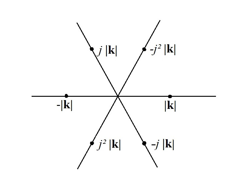
Figure 3: The six simple poles of the integral representation of zero-mass propagator of the sixth-order equation

In the case of the usual d’Alembertian several different Green’s functions can be obtained by taking the inverse Fourier transform of the (71), The most widely used is the retarded Green’s function, proportional to the well known expression

$$G_{ret}(x^{\mu})=Y(ct)\;\frac{\delta(ct-kr)}{4\pi r}$$ (72)

where $Y(ct)$ is Heaviside’s function.

In our case the Fourier transform of the Green function we are looking for is a product of three factors, namely we have to do with a product of three factors, namely:

$${\hat{G}}_{1}=\left[\frac{1}{k_{0}^{2}-\mid{\bf k}\mid^{2}}\right]\;\;\;{\hat{G}}_{2}=\left[\frac{j}{k_{0}^{2}-j\,\mid{\bf k}\mid^{2}}\right]\;\;{\rm and}\;\;\;{\hat{G}}_{3}=\left[\frac{j^{2}}{k_{0}^{2}-j^{2}\;\mid{\bf k}\mid^{2}}\right],$$ (73)

$$G(x^{\mu})=\frac{1}{16\pi^{4}}\;\int_{0}^{2\pi}d\varphi\int_{0}^{\pi}\sin\theta d\theta\int_{0}^{\infty}{\bf k}^{2}d\mid{\bf k}\mid\int_{-\infty}^{\infty}dk_{0}e^{-i(k_{0}ct-\mid{\bf k}\mid r\cos\theta)}\;{\hat{G}}(k^{\mu}),$$ (74)

With ${\hat{G}}(k^{\mu})$ given by the expression (70 or the product ${\hat{G}}_{1}\;{\hat{G}}_{2}\;{\hat{G}}_{3}$ (73). Qualitative picture is much easier to obtain i we use the latter form, because the inverse Fourier transform of a product is equal to the convolution of inverse Fourier transforms of each factor. And the inverse Fourier transforms of each of the three factors defined in (73) can be found using the standard integration procedure described in textbooks on Fourier transforms or in standard textbooks on electrodynamics ([20], [21]).

Each of its three factors contains an inverse of quadratic expression resembling the usual d’Alembertian, with $\mid{\bf k}^{2}\mid$ appearing with factors $1,\;j$ and $j^{2}$.

In what follows, we shall write $k$ instead of $\mid{\bf k}\mid$ when there is no risk of ambiguity. Supposing that $G(k^{\mu})$ is spherically symmetric, the integration over $d\varphi$ gives just the factor $2\pi$. Next, we can perform integration over $d\theta$, factorizing the only term depending on $\theta$, which is $e^{ikr\cos\theta}$. This integral gives

$$\int_{0}^{\pi}\;e^{ikr\cos\theta}\;\sin\theta d\theta=\int_{-1}^{1}\;e^{ikru}\,du=\frac{2\,\sin kr}{kr}.$$ (75)

What remains now is the integration over $dk$ and $dk_{0}$. As usual, the integral over $dk_{0}$ is taken first, and evaluated by extention to the complex domain. The first factor $G_{1}$ has two poles on the real line, $k_{0}=\pm\mid{\bf k}\mid$, and is evaluated as a principal value. The final result is the well known Green’s function of the d’Alembertian, 72. The remaining two factors are integrated over $dk_{0}$ even more easily, because their poles are found off the real axis, as shown in the following figure:

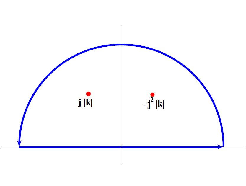
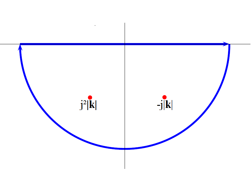
Figure 4: Left: The upper contour, containing the poles at $j\mid{\bf k}\mid$ and $-j^{2}\;\mid{\bf k}\mid$, for $t<0$; Right: The lower contour, containing the poles at $-j\mid{\bf k}\mid$ and $j^{2}\;\mid{\bf k}\mid$, for $t>0$ .

The resulting integrals yield the following expressions:

$$-2\pi i\;Y(t)\;\left[j\;e^{ijkct}-j^{2}\;e^{ij^{2}kct}\right]\;\;\;\;\;{\rm and}\;\;\;\;\;2\pi i\;Y(-t)\;\left[j^{2}\;e^{ij^{2}kct}-j\;e^{-ijkct}\right]$$ (76)

Substituting explicit expressions for all complex numbers appearing in these expressions, we get two real functions:

$$2\pi\;Y(t)\;e^{-\frac{\sqrt{3}}{2}kct}\;\left[\sqrt{3}\cos\frac{k}{2}ct+\sin\frac{k}{2}ct\right],\;\;\;\;2\pi\;Y(-t)\;e^{\frac{\sqrt{3}}{2}kct}\;\left[\sqrt{3}\cos\frac{k}{2}ct-\sin\frac{k}{2}ct\right],$$

Both expressions contain the damping factor $e^{\frac{\sqrt{3}}{2}kct}$ which is absent in the first contribution proportional to the usual d’Alembertian. But as all three components mix together, all will acquire these damping factors and fade away very quickly. These expressions multiply the Fourier transforms of each of the three $k$-dependent parts of Fourier images of Green’s function, $G_{2}$ and $G_{3}$, while the first one, $G_{1}$ similar to the usual d’Alembertian, has to be multiplied by $2\pi\;Y(t)\;\sin(kct)$. Before performing the last integration over $dk$, they should be multiplied by the factor $\frac{2\pi\;\sin(kr)}{kr}$.

The final results for each of the factors become, as could be expected, as follows:

$$G_{1}=Y(ct)\;\frac{\delta(kct-kr)}{r},\;\;\;G_{2}=Y(ct)\;\frac{\delta(kct-j^{2}\;kr)}{r},\;\;\;G_{3}=Y(ct)\;\frac{\delta(kct-j\;kr)}{r}.$$

and the Green’s function of the sixth-order massless operator can be obtained by the convolution of the three functions:

$$G(x^{\mu})=G_{1}*G_{2}*G_{3}.$$

The Dirac $\delta$-functions vanish everywhere except for the light cone $kct-kr=0$ in $G_{1}$, and for complex-valued wave vectors $k$ such that for $G_{2}(x^{\mu})$ $k$ must be proportional to $j$, and in the case of $G_{3}(x^{\mu})$ $k$ must be aligned along the $j^{2}$ axis.

After second quantization, these solutions can be implemented as operators with well-defined commutation properties. In order to reproduce the existing stable configurations of quarks of the first generation, $uud$ and $udd$, a generalized Pauli’s exclusion principle based on the $Z_{3}$ symmetry should replace the usual $Z_{2}$ symmetric exclusion principle, as proposed in [24], [25] and [26].

Acknowledgements      I am greatly indebted to Michel Dubois-Violette, Viktor Abramov and Karol Penson for many discussions and constructive criticism. I would like to express my sincere thanks to Jan-Willem van Holten, Jürg Frölich, Yuri Dokshitser, Paul Sorba and Reinald Flume for important discussions, suggestions and remarks. Thanks are due to Dr. Katarzyna Górska for her help with symbolic calculus.

References

References

[1] M. Gell-Mann, Y. Ne’eman, The Eightfold Way, Benjamin, New York (1964)
[2] H.J. Lipkin, Frontiers of the Quark Model, Weizmann
Inst. pr. WIS-87-47-PH (1987)
[3] S. Okubo, Journ. of Math. Physics, 34, 3273;
ibid , 3292 (1993)
[4] J. Scherk Rev. Mod. Phys. 47, 123 (1975)
[5] Madore J, Schraml S, P. Schupp P, Wess J, The European Physical Journal C, 16 (1), pp 161-167 (2000)
[19] Coleman S., Mandula J. Physical Review 159, p. 1251 (1967)
[20] Landau L.D, Lifshitz E.M, The Classical Theory of Fields, Third Revised edition, Pergamon Press (1971)
[21] Bremerman H., Distributions, Complex Variables and Fourier Transforms, Addison-Wesley, Mass., USA (1965)
[22] Kerner R 1991 Comptes Rendus Acad. Sci. Paris.10 pp. 1237-1240
[23] Kerner R Journal of Mathematical Physics, 33 (1) pp.403-4011 (1992)
[24] Kerner R in Symmetrties and Groups in Contemporary Physics, World Scientific,
eds. Chengming Bai, J.-P.Gazeau, Mo-Lin Ge), pp. 283-288 (2013)
[25] Kerner R Algebra, Geometry and Mathematical Physics, in Springer Proceedings series, Math.Stat., ed. A. Makhlouf and E. Paal,
85 pp. 617-637 (2014)
[26] Kerner R Physics of Atomic Nuclei80 (3), pp. 529-541 (2017)