Quantum Vacuum and the Structure of Empty Space-Time

Abstract

We have considered the possibility of formation a massless particles with spin 1 in the region of negative energies, within the framework of the Weyl type equation for neutrinos. It is proved that, unlike quantum electrodynamics, the developed approach allows in the ground state the formation of such stable particles. The structure and properties of this vector-boson are studied in detail. The problem of entangling two vector bosons with projections of spins +1 and -1 and, accordingly, the formation of a zero-spin boson is studied within the framework of a complex stochastic equation of the Langevin type. The paper discusses the structure of the Bose particle of a scalar field and the space-time’s properties of an empty space (quantum vacuum).

I Introduction

From a mathematical and philosophical point of view, the vacuum can be comparable with the region of absolutely empty space or, which is the same, with the region of the space where there are no massive particles and fields. From the physical point of view, the real vacuum is empty only ”on average”. Moreover, as it is known, due to the principle of quantum-mechanical uncertainty, there is not any way screening a certain area of space to exclude the appearance of virtual particles and fields in it. The Lamb Shift Lamb , Casimir effect Casimir , Unruh effect Unru , anomalous magnetic moment of electron Proh , Van der Waals forces Van , Delbrück scattering Del , Hawking radiation Haw , the cosmological constant problem Weinb ; Wein , vacuum polarization at weak electromagnetic fields Ash1 ; Ash2 - here is an incomplete list of phenomena, part of which has been experimentally discovered. All of them are conditioned by the physical vacuum or, more accurately, by a quantum vacuum (QV). The issues of quintessence (dark energy) and cosmic acceleration often are discussed in the framework of QV theories, which necessarily include scalar fields Wein . The properties of a quantum vacuum can be studied within the framework of quantum field theory (QFT), ie quantum electrodynamics and quantum chromodynamics (QCD). Note, that QFT could accurately describe QV if it were possible to exactly summarize the infinite series of perturbation theories, that is typical of field theories. However, it is well-known that the perturbation theory for QFT breaks down at low energies (for example, QCD or the BCS theory of superconductivity) field operators may have non-vanishing vacuum expectation values called condensates. Moreover, in the Standard Model precisely the non-zero vacuum expectation value of the Higgs field, arising from spontaneous symmetry breaking, is the principled mechanism allowing to acquire masses of other fields of theory.

To overcome these difficulties and to conduct a consistent and comprehensive study of the quantum vacuum, we developed a nonperturbative approach based on a system of complex stochastic equations of the Langevin type describing the motion of a massless particle with spin 1 in a random environment of similar particles.

The main objectives pursued by this study are as follows:

a. to study the possibility of formation a stable bound state of a massless particle with spin 1 (vector boson) in the region of negative energies,

b. to investigate the possibility of forming a massless particle with zero spin as a result of entangling the ground states of two vector bosons, respectively, with the projections of the spins 1 and -1,

c. to justify of the possibility the formation of a scalar field as a result of relaxation and Bose-Einstein (BEC) condensation of vector fields. To study the features the wave state of the boson of a scalar field, in particular, the possibility of its decay and spontaneous transitions to other vacuum and extravacuum states.

II Quantum motion of a photon in empty space

The questions of correspondence between the Maxwell equation and the equation of quantum mechanics was of interest to many researchers at the dawn of the development of quantum theory Opp ; Mol ; Wein1 .

As shown BIALYNICKI , the quantum motion of a photon in a vacuum can be considered within the framework of a wave function representation, writing it analogously to the Weyl equation for a neutrino in a vector form:

$$\partial_{t}\bm{\Psi^{+}}(\textbf{r},t)-c_{0}\bigl{(}\textbf{S}\cdot\bm{\nabla}\bigr{)}\bm{\Psi^{+}}(\textbf{r},t)=0,\qquad\qquad\qquad\,\,\,$$

$$\partial_{t}\bm{\Psi^{-}}(\textbf{r},t)+c_{0}\bigl{(}\textbf{S}\cdot\bm{\nabla}\bigr{)}\bm{\Psi^{-}}(\textbf{r},t)=0,\qquad\partial_{t}\equiv\partial/\partial t,$$ (1)

where $c_{0}$ denotes the speed of light in an empty $4D$ Minkowski space-time, $\bm{\Psi^{+}}(\textbf{r},t)$ and $\bm{\Psi^{-}}(\textbf{r},t)$ denote the photons wave functions of both helicities, corresponding to left-handed and right-handed polarizations. In addition, in (1) the set of matrices $\textbf{S}=(S_{x},S_{y},S_{x})$ describes infinitesimal rotations of particles with spin $\pm 1$, respectively:

$$S_{x}=\left[\begin{array}[]{ccc}0&0&0\\ 0&0&-i\\ 0&i&0\\ \end{array}\right],\qquad S_{y}=\left[\begin{array}[]{ccc}0&0&i\\ 0&0&0\\ -i&0&0\\ \end{array}\right],\,\,\,$$ (8)

$$S_{z}=\left[\begin{array}[]{ccc}0&-i&0\\ i&0&0\\ 0&0&0\\ \end{array}\right].\qquad\qquad\quad\,\,\,\,\,$$ (12)

Recall, that in (1) the absence of electrical and magnetic charges provides the following conditions:

$$\nabla\cdot\bm{\Psi^{\pm}}(\textbf{r},t)=0.$$ (13)

If we represent the wave function in the form:

$$\bm{\Psi^{\pm}}(\textbf{r},t)=\frac{1}{\sqrt{2}}\biggl{\{}\frac{\textbf{D}(\textbf{r},t)}{\sqrt{\epsilon_{0}}}\pm i\frac{\textbf{B}(\textbf{r},t)}{\sqrt{\mu_{0}}}\biggr{\}},\,\,c_{0}=\frac{1}{\sqrt{\mu_{0}\epsilon_{0}}},$$ (14)

then from the equations (1) and (13) it is easy to find Maxwell’s equations in an ordinary vacuum or in empty space:

$$\partial_{t}\textbf{D}-\nabla\times\textbf{H}=0,\qquad\nabla\cdot\textbf{E}=0,$$

$$\partial_{t}\textbf{B}+\,\nabla\times\textbf{E}=0,\qquad\nabla\cdot\textbf{H}=0,$$ (15)

where $\epsilon_{0}$ and $\mu_{0}$ describe the dielectric and magnetic constants of the vacuum, respectively. It is important to note that the dielectric and magnetic constants provide the following equations:

$$\textbf{D}=\epsilon_{0}\textbf{E},\qquad\textbf{B}=\mu_{0}\textbf{H}.$$

Recall that the only difference between the equations (1) and (15) is that the Maxwell equations system does not take into account the spin of the photon, which will be important for further constructions. Since the refractive indices $\epsilon_{0}$ and $\mu_{0}$ are constants that do not depend on external fields, and characterize the state of unperturbed or ordinary vacuum, a reasonable idea arises, namely, to consider a vacuum or, more accurately, QV, as some energy environment with unusual properties and structure.

II.1 Vector fields and their fundamental particle

Let us make the following substitutions in the equations (1):

$$c_{0}\mapsto c(x,y,z,\tau),\qquad t\mapsto\tau(t),$$ (16)

where $c$ is the velocity of propagation of the field in the structural particle, which differs from the speed of light $c_{0}$ in a vacuum, $\tau$ is the chronological parameter of a closed quantum system (internal time), which, naturally, must be quasi-periodic, and in the most general case can be represented as:

$$\tau(t)=T(t)\sin(t/T(t)),\qquad-\infty<t<+\infty,$$ (17)

where $T(t)>0$ is a bounded function-quasiperiod.

Proposition. The equations system (1)-(13), taking into account the remarks (16) and (17) describes the quantum states of the massless particles with spin projections $\pm 1$.

The particle of the vector field in depending on the value of the spin projection, can be described by one of the following sets of wave functions:

$$\bm{\psi}^{+}(\textbf{r},\tau)=\left[\begin{array}[]{ccc}\psi^{+}_{x}(\textbf{r},\tau)\\ \psi^{+}_{y}(\textbf{r},\tau)\\ \psi^{+}_{z}(\textbf{r},\tau)\\ \end{array}\right],\,\,\bm{\psi}^{-}(\textbf{r},\tau)=\left[\begin{array}[]{ccc}\psi^{-}_{x}(\textbf{r},\tau)\\ \psi^{-}_{y}(\textbf{r},\tau)\\ \psi^{-}_{z}(\textbf{r},\tau)\\ \end{array}\right],$$ (24)

which satisfy equations of the type (1)-(13) taking into account the above remarks.

Obviously, in the bound state, the 4D-interval of the propagated signal will be zero, and the points of the Minkowski space (events) are related to the relation, like the light cone:

$$s^{2}=c^{2}\tau^{2}-r^{2}=0,\qquad r^{2}=x^{2}+y^{2}+z^{2}.$$ (25)

Thus, the key question arises: can such equations describe the spatial localizations of massless fields, characteristic of a stable structured formations called a particles?

Substituting (24) into (1) and taking into account (12), we can find the following two independent system of first order partial differential equations:

$$ic^{-1}\partial_{\tau}\psi^{\pm}_{x}=\pm\partial_{y}\psi^{\pm}_{z}\mp\partial_{z}\psi^{\pm}_{y},$$

$$ic^{-1}\partial_{\tau}\psi^{\pm}_{y}=\pm\partial_{z}\psi^{\pm}_{x}\mp\partial_{x}\psi^{\pm}_{z},$$

$$ic^{-1}\partial_{\tau}\psi^{\pm}_{z}=\pm\partial_{x}\psi^{\pm}_{y}\mp\partial_{y}\psi^{\pm}_{x}.$$ (26)

In addition, the following relation can be found between the fields, taking into account the equation (13):

$$\partial_{x}{\psi}^{\pm}_{x}+\partial_{y}{\psi}^{\pm}_{y}+\partial_{z}{\psi}^{\pm}_{z}=0.$$ (27)

Since particles with spins $+1$ and $-1$ are symmetric in any sense, it is sufficient to study in detail only the wave function describing a particle with spin $+1$.

Using the equations (26) and (27) we can obtain the systems of second order partial differential equations for vacuum fields:

$$\square\psi^{+}_{x}={c}^{-1}{c_{,y}}\bigl{(}\partial_{x}\psi^{+}_{y}-\partial_{y}\psi^{+}_{x}\bigr{)}-{c}^{-1}{c_{,z}}\bigl{(}\partial_{z}\psi^{+}_{x}-\partial_{x}\psi^{+}_{z}\bigr{)}-c_{,\tau}c^{-3}\partial_{\tau}\psi^{+}_{x},$$

$$\square\psi^{+}_{y}={c}^{-1}{c_{,z}}\bigl{(}\partial_{y}\psi^{+}_{z}-\partial_{z}\psi^{+}_{y}\bigr{)}-{c}^{-1}{c_{,x}}\bigl{(}\partial_{x}\psi^{+}_{y}-\partial_{y}\psi^{+}_{x}\bigr{)}-c_{,\tau}c^{-3}\partial_{\tau}\psi^{+}_{y},$$

$$\square\psi^{+}_{z}={c}^{-1}{c_{,x}}\bigl{(}\partial_{z}\psi^{+}_{x}-\partial_{x}\psi^{+}_{z}\bigr{)}-{c}^{-1}{c_{,y}}\bigl{(}\partial_{y}\psi^{+}_{z}-\partial_{z}\psi^{+}_{y}\bigr{)}-c_{,\tau}c^{-3}\partial_{\tau}\psi^{+}_{z},$$ (28)

where $\square=\triangle-c^{-2}\partial_{\tau}^{2}$ denotes the D’Alembert operator, $\bigtriangleup$ is the Laplace operator, $c_{,\zeta}=\partial c/\partial\sigma$ and $\zeta=(x,y,z,\tau)$. To determine the explicit form of equations (28), we need to calculate the derivatives $c_{,\sigma}$. Using the equation (25), we can find:

$$c_{,\tau}=-\frac{c^{2}}{r},\quad c_{,x}=\frac{cx}{r^{2}},\quad c_{,y}=\frac{cy}{r^{2}},\quad c_{,z}=\frac{cz}{r^{2}}.$$ (29)

To continue the study of the problem, we need to reduce the system of equations (28) to the canonical form, when the field components are separated, and each of them is described by an autonomous equation.

Taking into account the circumstance that in this problem all fields are symmetric, the following additional conditions can be imposed on the field components:

$$(c_{,z}-c_{,y})\partial_{\tau}\psi^{+}_{x}=c_{,z}\partial_{\tau}\psi_{y}^{+}-c_{,y}\partial_{\tau}\psi_{z}^{+},$$

$$(c_{,x}-c_{,z})\partial_{\tau}\psi^{+}_{y}=c_{,x}\partial_{\tau}\psi_{z}^{+}-c_{,z}\partial_{\tau}\psi_{x}^{+},$$

$$(c_{,y}-c_{,x})\partial_{\tau}\psi^{+}_{z}=c_{,y}\partial_{\tau}\psi_{x}^{+}-c_{,x}\partial_{\tau}\psi_{y}^{+}.$$ (30)

It is easy to verify that these conditions are symmetric with respect to the components of the field and are given on the hypersurface of four-dimensional events. Further, using the conditions (30), the system of equations (28), can be reduced to the following canonical form:

$$\bigl{\{}\square+[i(c_{,z}-c_{,y})+c_{,\tau}c^{-1}]c^{-2}\partial_{\tau}\bigr{\}}\psi^{+}_{x}=0,$$

$$\bigl{\{}\square+[i(c_{,x}-c_{,z})+c_{,\tau}c^{-1}]c^{-2}\partial_{\tau}\bigr{\}}\psi^{+}_{y}=0,$$

$$\bigl{\{}\square+[i(c_{,y}-c_{,x})+c_{,\tau}c^{-1}]c^{-2}\partial_{\tau}\bigr{\}}\psi^{+}_{z}=0.$$ (31)

Note that unperturbed QV fields must satisfy the conditions of autonomy, that imply the separation of spatial and temporal components of the wave function. Proceeding from this, it is convenient to represent the wave function in the form:

$$\psi_{\sigma}^{+}(\textbf{r},\tau)=\exp{\Bigl{(}\frac{\mathcal{E}_{\sigma}\tau}{\hbar}\Bigr{)}}\phi_{\sigma}^{+}(\textbf{r}),\qquad\sigma=x,y,z,$$ (32)

where $\mathcal{E}_{\sigma}<0$ is the energy of the one mode of QV field. It is obvious that the symmetry of the problem implies the equality of the modes energies $\mathcal{E}_{x}=\mathcal{E}_{y}=\mathcal{E}_{z}=\mathcal{E}<0$.

Finally, substituting (32) into (31), taking into account (29), we can get the following system of equations:

$$\Bigl{\{}\triangle+\lambda\Bigl{[}-\lambda-\frac{1}{r}+i\frac{z-y}{r^{2}}\Bigr{]}\Bigr{\}}\phi_{x}^{+}(\textbf{r})=0,$$

$$\Bigl{\{}\triangle+\lambda\Bigl{[}-\lambda-\frac{1}{r}+i\frac{x-z}{r^{2}}\Bigr{]}\Bigr{\}}\phi_{y}^{+}(\textbf{r})=0,$$

$$\Bigl{\{}\triangle+\lambda\Bigl{[}-\lambda-\frac{1}{r}+i\frac{y-x}{r^{2}}\Bigr{]}\Bigr{\}}\phi_{z}^{+}(\textbf{r})=0,$$ (33)

where $\lambda=(\mathcal{E}/c\hbar)<0$, in addition, parameter $|\lambda|$ has dimensionality of inverse distance.

III The wave function of a massless particle with spin $+1$

Representing the wave function in the form:

$$\phi_{x}^{+}(\textbf{r})=\phi_{x}^{+(r)}(\textbf{r})+i\phi_{x}^{+(i)}(\textbf{r}),$$ (34)

from the first equation of the system (33), we can get the following two equations:

$$\Bigl{\{}\triangle-\lambda\Bigl{(}\lambda+\frac{1}{r}\Bigr{)}\Bigr{\}}\phi_{x}^{+(r)}(\textbf{r})-\lambda\frac{z-y}{r^{2}}\phi_{x}^{+(i)}(\textbf{r})=0,$$

$$\Bigl{\{}\triangle-\lambda\Bigl{(}\lambda+\frac{1}{r}\Bigr{)}\Bigr{\}}\phi_{x}^{+(i)}(\textbf{r})+\lambda\frac{z-y}{r^{2}}\phi_{x}^{+(r)}(\textbf{r})=0.$$ (35)

It can be verified that by using simple substitutions of unknowns $\phi_{x}^{+(r)}(\textbf{r})\mapsto\phi_{x}^{+(i)}(\textbf{r})$ and $\phi_{x}^{+(i)}(\textbf{r})\mapsto-\phi_{x}^{+(r)}(\textbf{r})$, these equations pass into each other. The latter means that the solutions in modulus are equal and differ only in sign. In other words, the symmetry properties mentioned above make it possible to obtain two independent equations of the form:

$$\Bigl{\{}\triangle-\lambda\Bigl{[}\lambda+\frac{r-y+z}{r^{2}}\Bigr{]}\Bigr{\}}\phi_{x}^{+(r)}(\textbf{r})=0,$$

$$\Bigl{\{}\triangle-\lambda\Bigl{[}\lambda+\frac{r+y-z}{r^{2}}\Bigr{]}\Bigr{\}}\phi_{x}^{+(i)}(\textbf{r})=0.$$ (36)

Now we analyze the possibility of solving for the term $\phi_{x}^{+(r)}(\textbf{r})$ in the form of a localized state. Let us consider the following equation:

$$r-y+z=\mu r,$$ (37)

where $\mu$ is a some parameter. The changing range of this parameter will be defined below.

Substituting (37) into the first equation of the system (36), we get:

$$\Bigl{\{}\triangle+\bigl{[}-\lambda^{2}-\lambda\mu{r}^{-1}\bigr{]}\Bigr{\}}\phi_{x}^{+(r)}(\textbf{r})=0.$$ (38)

To continue the research, it is useful to rewrite the equation (38) in the spherical coordinates system $(x,y,z)\mapsto(r,\theta,\varphi)$:

$$\biggl{\{}\frac{1}{r^{2}}\Bigl{[}\frac{\partial}{\partial r}\Bigl{(}r^{2}\frac{\partial}{\partial r}\Bigr{)}+\frac{1}{\sin^{2}\theta}\frac{\partial^{2}}{\partial\varphi^{2}}+\frac{1}{\sin\theta}\frac{\partial}{\partial\theta}\Bigl{(}\sin\theta\frac{\partial}{\partial\theta}\Bigr{)}\Bigr{]}-\lambda^{2}\Bigl{[}1-\frac{\mu(\theta,\varphi)}{\lambda r}\Bigr{]}\biggr{\}}\phi_{x}^{+(r)}=0.$$ (39)

Using for the wave function the representation:

$$\phi_{x}^{+(r)}(\textbf{r})=\Lambda(r)Y(\theta,\varphi),$$ (40)

we can conditionally separate the variables in the equation (47) and write it in the form of the following two equations:

$$r^{2}\Lambda^{{}^{\prime\prime}}+2r\Lambda^{{}^{\prime}}+\bigl{[}-\lambda^{2}r^{2}-\lambda\mu(\theta,\varphi)r-\nu\bigr{]}\Lambda=0,$$ (41)

and, respectively;

$$\frac{1}{\sin\theta}\Bigl{\{}\frac{1}{\sin\theta}\frac{\partial^{2}}{\partial\varphi^{2}}+\frac{\partial}{\partial\theta}\Bigl{(}\sin\theta\frac{\partial}{\partial\theta}\Bigr{)}\Bigr{\}}Y+\nu Y=0,$$ (42)

where $\Lambda^{{}^{\prime}}=d\Lambda/dr$ and $\nu$ is a constant, which is convenient to represent in the form $\nu=l(l+1)$ and $l=0,1,2...$ Recall that the conditional separation of variables means to impose an additional condition on the function $\mu(\theta,\varphi)=const$. Writing equation (37) in spherical coordinates, we obtain the following trigonometric equation:

$$\mu(\theta,\varphi)=1-\sin\theta\sin\varphi+\cos\theta.$$ (43)

As the analysis of the equation (43) shows, the range of variation of the parameter $\mu$ for real angles is $\mu\in[(1-\sqrt{2}),(1+\sqrt{2})]$.

The solution of the equation (42) is well known, these are spherical Laplace functions $Y_{l}^{m}(\theta,\varphi)$ and $m=0,\pm 1,...,\pm l$.

As for the equation (41), we will solve it for a fixed value $\mu$, which is equivalent to the plane cut of the three-dimensional solution. In particular, we will seek a solution $\Lambda(r)$ tending to finite value for $r\to 0$ and, respectively, to zero at $r\to\infty$.

For a given parameter $\mu_{0}$, we can write the equation (41) in the form:

$$\frac{d^{2}\Lambda}{d\varrho^{2}}+\frac{2}{\varrho}\frac{d\Lambda}{d\varrho}+\Bigl{[}-\beta^{2}+\frac{2}{\varrho}-\frac{l(l+1)}{\varrho^{2}}\Bigr{]}\Lambda=0,$$ (44)

where $\varrho=r/a_{p}$ is a dimensionless distance, $a_{p}=2/(|\lambda|\mu_{0})$ denotes the characteristic spatial dimension of a hypothetical massless Bose particle with spin 1 and $\beta=2/\mu_{0}$. As can be seen, this equation describes the radial wave function of a hydrogen-like system Land . Recall that it can have a solution describing the bound state if the following condition is satisfied:

$$n_{r}+l+1=n+l=\frac{1}{\beta},\qquad n_{r}=0,1,2...,$$ (45)

where $n_{r}$ is the radial quantum number, and $n$, respectively, is the principal quantum number.
It is easy to see that there is only one integer $\mu_{0}=2$ for which $\beta=1$ and, accordingly, the equation (45) has a solution. In other words, the equality $\mu_{0}=2$ is a necessary quantization condition, which, with consideration (43), is equivalent to the trigonometric equation:

$$1+\sin\theta\sin\varphi-\cos\theta=0.$$ (46)

In particular, from this condition it follows that the $\Lambda(r)$ solution of the equation (44) is localized on the plane $S^{r}_{x}(\theta,\varphi)\cong(-Y,Z)$ (see FIG. 1).

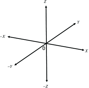
Figure 1: The coordinate system $\{X,Y,Z\}$ divides the 3D space into eight spatial regions using twelve planes. The boson of a vector field with spin projection +1 is a 2D-string (brane) consisting of six components localized on the following planes $\phi^{+}_{x}[(-Y,Z)\cup(Y,-Z)],$ $\phi^{+}_{y}[(-X,Z)\cup(X,-Z)]$ and $\phi^{+}_{z}[(-X,Y)\cup(X,-Y)]$, respectively.

Proceeding from the foregoing, we can write the solution of equation (44) on this plane:

$$\phi^{r}_{x}(r,\theta,\varphi)=\Lambda_{nl}(r)Y_{l}^{m}(\theta,\varphi),$$

which, subject to the condition (46), has a solution only for the ”ground state”:

$$\Lambda_{10}(r)=\frac{C}{\sqrt{a_{p}^{3}}}\,e^{-r/a_{p}},\qquad Y_{0}^{0}(\theta,\varphi)=\frac{1}{2}\sqrt{\frac{1}{\pi}},$$ (47)

where $C$ denotes a constant, which will be defined below from the normalization condition of the wave function. It is easy to see that the additional condition $\mu(\theta,\varphi)=\mu_{0}=2$ does not lead to a contradiction between the equations (41) and (42), and the solution (47) is the only solution of the first equation in the system (35) in the region of negative energies.

The imaginary part of the wave function is calculated similar way, but in this case we obtain following underdetermined trigonometric equation:

$$1-\sin\theta\sin\varphi+\cos\theta=0,$$ (48)

which determines the plane $S^{i}_{x}(\theta,\varphi)\cong(Y,-Z)$ on which the solution of the ground state is localized.

Similar solutions are obtained for the projections of the wave function $\phi^{+}_{y}$ and $\phi^{+}_{z}$. In this case, however, the components of the wave function $\bm{\phi}^{+}(\textbf{r})$ are localized on the planes $\{S^{r}_{y}(\theta,\varphi)\cong(-X,Z),\,\,S^{i}_{y}(\theta,\varphi)\cong(X,-Z)\}$ and $\{S^{r}_{z}(\theta,\varphi)\cong(X,-Y),\,\,S^{i}_{z}(\theta,\varphi)\cong(-X,Y)\}$, accordingly. So, the orient of first pair of planes $(S^{r}_{y},\,\,S^{i}_{y})$ are determined by the equations:

$$1\pm\cos\theta\sin\varphi\mp\cos\theta=0,$$ (49)

while, the orientations of the second pair of planes $(S^{r}_{z},\,\,S^{i}_{z})$ are given by the equations:

$$1\pm\sin\theta\sin\varphi\mp\cos\theta\sin\varphi=0.$$ (50)

It should be noted that the coefficient of the radial wave function (see (47)) is chosen so that the total vector wave function $\bm{\psi}^{+}$ of the ”ground state” is normalized to unity.

Now we can write down the normalization condition for the total wave function for the vector boson:

$$J=\int\bm{\phi}^{+}\bigl{(}\bar{\bm{\phi}}^{+}\bigr{)}^{T}dV=1,\qquad dV=dxdydz,$$ (51)

where $\bigl{(}\bar{\bm{\phi}}^{+}\bigr{)}^{T}=\bigl{(}\bar{\bm{\phi}}^{+}_{x},\bar{\bm{\phi}}^{+}_{y},\bar{\bm{\phi}}^{+}_{z}\bigr{)}$ is the transposed vector.
We can represent the integral (51) as a sum of three terms:

$$J=\int\phi^{+}_{x}\bar{\phi}^{+}_{x}dV+\int\phi^{+}_{y}\bar{\phi}^{+}_{y}dV+\int\phi^{+}_{z}\bar{\phi}^{+}_{z}dV.$$ (52)

It is obvious that all terms in the expression (52) are equal and, therefore, each of them is equal to 1/3.

As an example, consider the first summand. Taking into account that the wave function can be represented in the form $\phi^{+}_{x}=\phi^{+(r)}_{x}+i\phi^{+(i)}_{x}$, and its components $\phi^{+(r)}_{x}$ and $\phi^{+(i)}_{x}$, are localized in a region that is the union of two quaternary planes ${(-Y,Z)\cup(Y,-Z)}\subset(Y,Z)$, we can write:

$$\int\phi^{+}_{x}\bar{\phi}^{+}_{x}dV=\int\bigl{(}|\phi^{+(r)}_{x}|^{2}+|\phi^{+(i)}_{x}|^{2}\bigr{)}dV=2\int|\phi^{+(r)}_{x}|^{2}dV=2\int|\phi^{+(i)}_{x}|^{2}dV=\frac{a_{p}}{2\pi}\int_{(-Y,Z)}|\Lambda_{10}(\rho)|^{2}dydz=1/3.$$ (53)

where $\varrho=r(0,y,z)=\sqrt{y^{2}+z^{2}}$ denotes radius-vector $r$ on the plane $(-Y,Z)$, in addition, in calculating the integral, we assume that the wave function in perpendicular to the plane $(-Y,Z)$ direction $x$ is the Dirac delta function.

Taking into account (47), we can accurately calculate the integral in the expression (53):

$$\int_{(-Y,Z)}|\Lambda_{10}(\rho)|^{2}dydz=\frac{\pi}{8a_{p}}C^{2}.$$ (54)

Now using (53) and (54), we can determine the normalization constant of the wave function (47), which is equal to $C=4/\sqrt{3}$. Note that similarly we can find a solution of the boson wave function with the spin projection -1 (see Appendix A).

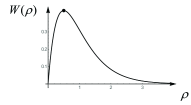
Figure 2: The distance $\rho_{0}=1/2$, or more precisely $\varrho_{0}=a_{p}/2$, at which the maximum value of the amplitude of the brane probability is reached.

Finally, we turn to the characteristic scale of the brane, which, as follows from the quantization condition (see (44)-(45)), is defined by the equation:

$$a_{p}=\frac{1}{|\lambda|}=\frac{c\hbar}{|\mathcal{E}|},$$ (55)

where $c$ is the speed of propagation of a wave in the brane, which can significantly differ from the speed of light in a vacuum. Unfortunately, it is impossible to determine $a_{p}$ from equation (44). Nevertheless, if we assume that the spatial scale brane has the Planck length $l_{P}$, ie, $a_{p}=l_{P}=1,616,229(38)\cdot 10^{-33}sm$, and the energy particle is $-1MeV$, then the propagation velocity of the wave in the brane will be equal to $c=3,86\cdot 10^{-13}sm/s$.

Using the solution of the ground state, on the corresponding planes, we can calculate the location of the maximum probability of one of the projections of the brane. The probability of finding the maximum amplitude of the projection of a brane wave into an element of the area $dS=rdrd\vartheta$ can be determined as follows:

$$dW(\rho)={C^{\prime}}^{2}e^{-2\rho}{\rho}d{\rho}d\vartheta,\qquad C^{\prime}=C/\sqrt{a_{p}^{3}},$$ (56)

where $\vartheta\in[0,\pi/2].$
Investigating the expression $dW/d\rho$, it is easy to find that for the value $\rho=1/2$ and, respectively, for $r(0,x,y)=\varrho=a_{p}/2$, the probability distribution has a maximum FIG 2. Proposition is proved.

IV Formation of a scalar field

Let us consider QV, taking into account the fluctuations of the vector fields. As the basic equations we will use the system of stochastic matrix equations of the Langevin type:

$$\partial_{t}\bm{\breve{{\psi}}^{+}}(\textbf{r}_{+},t)-c\bigl{(}\textbf{S}\cdot\bm{\nabla}\bigr{)}\bm{\breve{{\psi}}^{+}}(\textbf{r}_{+},t)=\bm{\eta}^{+}(s_{+}),$$

$$\partial_{t}\bm{\breve{{\psi}}^{-}}(\textbf{r}_{-},t)+\,c\bigl{(}\textbf{S}\cdot\bm{\nabla}\bigr{)}\bm{\breve{{\psi}}^{-}}(\textbf{r}_{-},t)=\bm{\eta}^{-}(s_{-}),$$ (57)

and also the equations:

$$\nabla\bm{\breve{{\psi}}^{+}}(\textbf{r}_{+},t)=0,\qquad\nabla\bm{\breve{{\psi}}^{-}}(\textbf{r}_{-},t)=0,$$ (58)

where $\textbf{r}_{\pm}$ denotes the radius-vector of corresponding vector particles, $t\in(-\infty,+\infty)$ is a usual time. In equation (57) complex stochastic generators $\bm{\eta}^{\pm}(s_{\pm})=(\eta_{x}^{\pm},\eta_{y}^{\pm},\eta_{z}^{\pm})$, describing random charges and currents arising in 4D-intervals $ds^{2}_{\pm}=c^{2}dt^{2}-dx^{2}_{\pm}-dy^{2}_{\pm}-dz^{2}_{\pm}$.

For further research, it is useful to write these equations in matrix form:

$$\left[\begin{array}[]{ccc}\vspace{2mm}ict&-z_{+}&y_{+}\\ \vspace{2mm}z_{+}&ict&-x_{+}\\ \vspace{2mm}-y_{+}&x_{+}&ict\\ \end{array}\right]\cdot\left[\begin{array}[]{ccc}\vspace{0.7mm}\dot{\breve{{\psi}}}_{x}^{+}\\ \vspace{0.7mm}\dot{\breve{{\psi}}}_{y}^{+}\\ \vspace{0.7mm}\dot{\breve{{\psi}}}_{z}^{+}\\ \end{array}\right]=s_{+}\left[\begin{array}[]{ccc}\vspace{2mm}\eta_{x}^{+}\\ \vspace{2mm}\eta_{y}^{+}\\ \vspace{2mm}\eta_{z}^{+}\\ \end{array}\right],\quad$$

and, respectively,

$$\left[\begin{array}[]{ccc}\vspace{2mm}ict&z_{-}&-y_{-}\\ \vspace{2mm}-z_{-}&ict&x_{-}\\ \vspace{2mm}y_{-}&-x_{-}&ict\\ \end{array}\right]\cdot\left[\begin{array}[]{ccc}\vspace{0.7mm}\dot{\breve{{\psi}}}_{x}^{-}\\ \vspace{0.7mm}\dot{\breve{{\psi}}}_{y}^{-}\\ \vspace{0.7mm}\dot{\breve{{\psi}}}_{z}^{-}\\ \end{array}\right]=s_{-}\left[\begin{array}[]{ccc}\vspace{2mm}\eta_{x}^{-}\\ \vspace{2mm}\eta_{y}^{-}\\ \vspace{2mm}\eta_{z}^{-}\\ \end{array}\right],$$ (68)

where $\dot{\breve{{\psi}}}_{\sigma}^{\varsigma}=\partial\breve{{\psi}}_{\sigma}^{\varsigma}/\partial s_{\varsigma}$, in addition, the following notations are made $\varsigma=(+,-)$ and $\sigma=(x,y,z).$

In addition, from (13) we can find the following two relations between the stochastic components of the wave function:

$$x_{+}\dot{\breve{{\psi}}}^{+}_{x}+y_{+}\dot{\breve{{\psi}}}^{+}_{y}+z_{+}\dot{\breve{{\psi}}}^{+}_{z}=0,$$

$$x_{-}\dot{\breve{{\psi}}}^{-}_{x}+y_{-}\dot{\breve{{\psi}}}^{-}_{y}+z_{-}\dot{\breve{{\psi}}}^{-}_{z}=0.$$ (69)

For the further analytical study of the problem, it is important to reduce the system of equations (68) to the canonical form:

$$\dot{\breve{{\psi}}}^{+}_{\sigma}(s_{+};\textbf{r}_{+},t)=\bigl{\{}b^{+}_{\sigma}(\textbf{r}_{+},t)+d^{+}_{\sigma}(\textbf{r}_{+},t)\bigr{\}}\bar{s}^{-1}_{+}\eta^{+}(s_{+}),\quad$$

$$\dot{\breve{{\psi}}}^{-}_{\sigma}(s_{-};\textbf{r}_{-},t)=\bigl{\{}b^{-}_{\sigma}(\textbf{r}_{-},t)+d^{-}_{\sigma}(\textbf{r}_{-},t)\bigr{\}}\bar{s}^{-1}_{-}\eta^{-}(s_{-}),\quad$$ (70)

where $\bar{s}_{+}=s_{+}/a_{p}$ and $\bar{s}_{-}=s_{-}/a_{p}$, in addition, the following notations are made:

$$b^{\varsigma}_{x}(\textbf{r}_{\varsigma},t)=(z_{\varsigma}-y_{\varsigma})/a_{p},\qquad\qquad\qquad\qquad\,\,$$

$$b^{\varsigma}_{y}(\textbf{r}_{\varsigma},t)=(x_{\varsigma}-z_{\varsigma})/a_{p},\qquad\qquad\qquad\qquad\,\,$$

$$b^{\varsigma}_{z}(\textbf{r}_{\varsigma},t)=(y_{\varsigma}-x_{\varsigma})/a_{p},\qquad\qquad\qquad\qquad\,\,$$

$$d_{x}^{\varsigma}(\textbf{r}_{\varsigma},t)=(c^{2}t^{2}-x^{2}_{\varsigma}-x_{\varsigma}y_{\varsigma}-x_{\varsigma}z_{\varsigma})/(a_{p}ct),$$

$$d^{\varsigma}_{y}(\textbf{r}_{\varsigma},t)=(c^{2}t^{2}-y^{2}_{\varsigma}-x_{\varsigma}y_{\varsigma}-y_{\varsigma}z_{\varsigma})/(a_{p}ct),$$

$$d^{\varsigma}_{z}(\textbf{r}_{\varsigma},t)=(c^{2}t^{2}-z^{2}_{\varsigma}-x_{\varsigma}z_{\varsigma}-y_{\varsigma}z_{\varsigma})/(a_{p}ct).$$ (71)

Note that when deriving the equations (71) - (70) we assumed that the following relations hold:

$$\eta_{x}^{\varsigma}=\eta_{y}^{\varsigma}=\eta_{z}^{\varsigma}=\eta^{\varsigma},\qquad d\bar{s}_{+}=d\bar{s}_{-}=d\bar{s},$$

which looks quite natural in the context of considered problem.

Now we will assume that the random generators satisfy the following correlation properties:

$$\langle\eta(\bar{s})\rangle=0,\qquad\langle\eta(\bar{s})\eta(\bar{s}^{\prime})\rangle=2\varepsilon\delta(\bar{s}-\bar{s}^{\prime}),$$ (72)

where $\eta(\bar{s})=\bar{s}^{-1}\eta^{-}(\bar{s})=\bar{s}^{-1}\eta^{+}(\bar{s})$ and $\varepsilon=(\varepsilon^{r}+i\varepsilon^{i})$ is a complex constant denoting the fluctuation power; in addition, we assume that $\varepsilon_{0}=\varepsilon^{r}=\varepsilon^{i}.$

We can represent the joint probability distribution of fields in the form (see AshG ):

$$\mathcal{P}(\{\breve{\psi}\},\bar{s};\textbf{r}_{+},\textbf{r}_{-},t)=\prod_{\varsigma,\sigma}\bigl{\langle}\delta\bigl{(}\breve{\psi}_{\sigma}^{\varsigma}(\bar{s};\textbf{r}_{\varsigma},t)-\psi_{\sigma}^{\varsigma}\bigr{)}\bigr{\rangle},$$ (73)

where $\{{\breve{\psi}}\}=({\breve{\psi}}^{+}_{x},...,{\breve{\psi}}^{-}_{z})$ denotes a set of fluctuations of vacuum fields and $\psi_{\sigma}^{\varsigma}=\breve{\psi}_{\sigma}^{\varsigma}(s)|_{t=0}$. In the (73) $\delta(\breve{\psi}_{\sigma}^{\varsigma}(s;\textbf{r}_{\varsigma},t)-\psi_{\sigma}^{\varsigma})$, denotes the Dirac delta function generalized on a 6D-Hilbert space, in addition, by default we will assume that the wave function is dimensionless, that is, it is multiplied by a constant value $a_{p}^{3/2}$ (see (47)).

Using the system of stochastic equations (70), for the conditional probability the following second order partial differential equation can be obtained (see Ashg1 ):

$$\Bigl{\{}\frac{\partial}{\partial\bar{s}}-\frac{1}{2}\sum_{\varsigma,\sigma}\varepsilon_{\sigma}^{\varsigma}(\textbf{r}_{\varsigma},t)\frac{\partial^{2}}{\partial{\breve{\psi}}_{\sigma}^{\varsigma}\partial\bar{\breve{\psi}}_{\sigma}^{\varsigma}}\Bigr{\}}\mathcal{P}=0,$$ (74)

where $\bar{\breve{\psi}}_{\sigma}^{\varsigma}$ denotes the complex conjugate of the function $\breve{\psi}_{\sigma}^{\varsigma}$ and $\varepsilon_{\sigma}^{\varsigma}(\textbf{r}_{\varsigma},t)=\varepsilon_{0}[b_{\sigma}^{\varsigma}(\textbf{r}_{\varsigma},t)+d_{\sigma}^{\varsigma}(\textbf{r}_{\varsigma},t)]^{2}$, which is a dimensionless quantity and denotes fluctuations power.

Recall that in the equation (74) the following notation is used:

$$\frac{\partial^{2}}{\partial{\breve{\psi}}_{\sigma}^{\varsigma}\partial\bar{\breve{\psi}}_{\sigma}^{\varsigma}}=\frac{\partial^{2}}{\partial\bigl{[}{\breve{\psi}}_{\sigma}^{\varsigma(r)}\bigr{]}^{2}}+\frac{\partial^{2}}{\partial\bigl{[}{\breve{\psi}}_{\sigma}^{\varsigma(i)}\bigr{]}^{2}},$$

where $\breve{\psi}_{\sigma}^{\varsigma(r)}=\emph{Re}(\breve{\psi}_{\sigma}^{\varsigma})$ and $\breve{\psi}_{\sigma}^{\varsigma(i)}=\emph{Im}(\breve{\psi}_{\sigma}^{\varsigma})$.

For further it is convenient to represent the general solution of the equation (74) in the following integral form:

$$\mathcal{P}(\{\breve{\psi}\},\bar{s}\,;\textbf{r}_{+},\textbf{r}_{-},t)=\int_{\Xi^{6}}\mathcal{{P}}_{0}(\{\psi_{0}\})\prod_{\varsigma,\sigma}\exp\biggl{\{}-\frac{(\psi_{\sigma}^{\varsigma}-{\breve{\psi}}_{\sigma}^{\varsigma})(\bar{\psi}_{\sigma}^{\varsigma}-\bar{{\breve{\psi}}}_{\sigma}^{\varsigma})}{2\bar{s}\varepsilon_{\sigma}^{\varsigma}}\biggr{\}}\frac{d\psi_{\sigma}^{\varsigma}}{\sqrt{2\pi\bar{s}\varepsilon_{\sigma}^{\varsigma}}},\qquad d\psi_{\sigma}^{\varsigma}=d\psi_{\sigma}^{\varsigma(r)}d\psi_{\sigma}^{\varsigma(i)},$$ (75)

where $\mathcal{{P}}_{0}(\{\psi_{0}\})$ denotes an initial condition of the equation (74) at $t=0$, before including of interaction with the random environment. Recall that the integration over the 6D Hilbert space $\Xi^{6}$, ie by the spectrum, in accordance with the ergodic hypothesis, is equivalent in this case to integration over the full 12D configuration space. Note that the integration in (75) should be understood as an integral operator that acts on each element of the matrix, which, as we shall show below, is the $\mathcal{{P}}_{0}(\{\psi_{0}\})$.

On the basis of physical considerations, as an initial condition, we can choose the probability density of the ”ground state” of a scalar field’s particle, which can be formed by two vector bosons with projections of spin $+1$ and $-1$, respectively. It is obvious that the probability density $\mathcal{P}$ should be normalized on the unit matrix of the size $I_{3}=3\times 3$:

$$\int_{\Xi^{6}}\mathcal{P}(\{\bm{\breve{}}{\psi}\},\bar{s}\,;\textbf{r}_{+},\textbf{r}_{-},t)\prod_{{\varsigma},{\sigma}}d{\breve{\psi}}_{{\sigma}}^{\varsigma}=I_{3}.$$ (76)

Substituting $(\ref{4.03a})$ into $(\ref{4.03bt})$ and integrating over variables within $\bigr{[}\breve{\psi}_{\sigma}^{\varsigma(r)},\,\breve{\psi}_{\sigma}^{\varsigma(i)}\bigl{]}\in(-\infty,+\infty)$, we get the following condition for the density matrix $\mathcal{{P}}_{0}(\{\psi_{0}\})$:

$$\int_{\Xi^{6}}\mathcal{{P}}_{0}(\{\psi_{0}\})\prod_{\varsigma,\sigma}d{\psi}_{\sigma}^{\varsigma}=I_{3}.$$ (77)

The wave function of a scalar field particle (scalar boson with spin-0) can be represented as the maximally entangled state of two ”ground states” of the vector field particles (EPR state Einst ):

$$\bm{\psi}^{\updownarrow}(\textbf{r}_{+},\textbf{r}_{-},0)=\frac{1}{\sqrt{2}}\bigl{\{}|\uparrow\rangle_{1}\otimes|\downarrow\rangle_{2}-|\downarrow\rangle_{1}\otimes|\uparrow\rangle_{2}\bigr{\}},$$ (78)

where we make the following notation: $|\uparrow\rangle_{1}=\bm{\phi}^{+}(\textbf{r}_{+})$ and $|\downarrow\rangle_{2}=\bm{\phi}^{-}(\textbf{r}_{-})$, while $|\downarrow\rangle_{1}=\bm{\bar{}}{\phi}^{+}(\textbf{r}_{+})$ and $|\uparrow\rangle_{2}=\bm{\bar{}}{\phi}^{-}(\textbf{r}_{-})$. Note that the wave function (78) denotes one of Bell’s entangled states of four possible Bell . Recall that in the equation (78) the symbol $\otimes$ denotes the operation of a direct (tensor) product:

$$\textbf{A}=|\uparrow\rangle_{1}\otimes|\downarrow\rangle_{2}=\left[\begin{array}[]{ccc}\vspace{1mm}{\phi}_{x}^{+}\\ \vspace{1mm}{\phi}_{y}^{+}\\ \vspace{1mm}{\phi}_{z}^{+}\\ \end{array}\right]\left[\begin{array}[]{ccc}{\phi}_{x}^{-}\,\,{\phi}_{y}^{-}\,\,{\phi}_{z}^{-}\end{array}\right],\quad\,$$

$$\bar{\textbf{A}}=|\downarrow\rangle_{1}\otimes|\uparrow\rangle_{2}=\left[\begin{array}[]{ccc}\vspace{1mm}{\bar{\phi}}_{x}^{+}\\ \vspace{1mm}{\bar{\phi}}_{y}^{+}\\ \vspace{1mm}{\bar{\phi}}_{z}^{+}\\ \end{array}\right]\left[\begin{array}[]{ccc}{\bar{\phi}}_{x}^{-}\,\,{\bar{\phi}}_{y}^{-}\,\,{\bar{\phi}}_{z}^{-}\end{array}\right],$$ (83)

where A denotes the third-rank matrix, while $\bar{\textbf{A}}$ its complex conjugation. The wave function of the boson of a scalar field can be represented in the form of a difference of two matrices (see Appendix B):

$$\bm{\psi}^{\updownarrow}(\textbf{r}_{+},\textbf{r}_{-},0)=\frac{1}{\sqrt{2}}\bigl{\{}\textbf{A}-\bar{\textbf{A}}\}=\frac{1}{\sqrt{2}}\,\textbf{B}=\quad$$

$$\frac{1}{\sqrt{2}}\left[\begin{array}[]{ccc}\vspace{1mm}B_{11}\,\,\,B_{12}\,\,\,B_{13}\\ \vspace{1mm}B_{21}\,\,\,B_{22}\,\,\,B_{23}\\ \vspace{1mm}B_{31}\,\,\,B_{32}\,\,\,B_{33}\\ \end{array}\right]=\frac{1}{\sqrt{2}}\left[\begin{array}[]{ccc}\vspace{1mm}B_{11}\,\,\,0\,\,\,\,0\\ \vspace{1mm}0\quad B_{22}\,\,\,\,0\\ \vspace{1mm}\,\,0\quad\,0\,\,\,\,\,B_{33}\\ \end{array}\right],\,\,$$ (90)

where the elements $B_{ij}=A_{ij}-\bar{A}_{ij}$ of the matrix B are calculated explicitly:

$$B_{11}=2i\bigl{[}\phi^{+(i)}_{x}\phi^{-(r)}_{x}-\phi^{+(r)}_{x}\phi^{-(i)}_{x}\bigr{]},$$

$$B_{22}=2i\bigl{[}\phi^{+(i)}_{y}\phi^{-(r)}_{y}-\phi^{+(r)}_{y}\phi^{-(i)}_{y}\bigr{]},$$

$$B_{33}=2i\bigl{[}\phi^{+(i)}_{z}\phi^{-(r)}_{z}-\phi^{+(r)}_{z}\phi^{-(i)}_{z}\bigr{]}.$$ (91)

Recall that the matrix elements $B_{ij}$ for $i\neq j$ are equal to zero, since the localization domains of the functions occurring in them have no intersection.

The distribution of the probability in a scalar field’s boson before switching-on of the random environment has the form:

$$\mathcal{{P}}_{0}(\{\psi_{0}\})=\frac{1}{C_{0}}\bigl{|}\bigr{|}\bm{\psi}^{\updownarrow}(\textbf{r}_{+},\textbf{r}_{-},0)\bigr{|}\bigr{|}^{2}=\frac{1}{2C_{0}}\,\textbf{C},$$ (92)

where $C_{0}$ is the constant that will be found from the normalization condition for the probability density on the matrix $I_{3}$, in addition:

$$\textbf{C}=\textbf{B}\cdot\textbf{B}=\left[\begin{array}[]{ccc}\vspace{1mm}C_{11}\,\,\,\,0\,\,\,\,0\\ \vspace{1mm}0\quad C_{22}\,\,\,0\\ \vspace{1mm}\,\,0\quad\,0\,\,\,\,C_{33}\\ \end{array}\right],$$

is a diagonal third rank matrix, the elements of which have the following form:

$$C_{11}=B_{11}\bar{B}_{11},\quad C_{22}=B_{22}\bar{B}_{22},\quad C_{33}=B_{33}\bar{B}_{33},$$

$$C_{13}=C_{12}=C_{23}=C_{32}=0.\qquad\qquad$$ (93)

Taking into account the fact that the spins of the vector bosons $\bm{\phi}^{+}$ and $\bm{\phi}^{-}$ lie on one axis but directed an opposite, for elements of the matrix C we obtain the following expressions:

$$C_{11}=4\bigl{[}\phi^{+(r)}_{x}\phi^{-(i)}_{x}\bigr{]}^{2}+4\bigl{[}\phi^{+(i)}_{x}\phi^{-(r)}_{x}\bigr{]}^{2},$$

$$C_{22}=4\bigl{[}\phi^{+(r)}_{y}\phi^{-(i)}_{y}\bigr{]}^{2}+4\bigl{[}\phi^{+(i)}_{y}\phi^{-(r)}_{y}\bigr{]}^{2},$$

$$C_{33}=4\bigl{[}\phi^{+(r)}_{z}\phi^{-(i)}_{z}\bigr{]}^{2}+4\bigl{[}\phi^{+(i)}_{z}\phi^{-(r)}_{z}\bigr{]}^{2}.$$ (94)

Substituting $(\ref{4.03bz})$ into $(\ref{4.03bt})$ and integrating, we can obtain:

$$\int_{\Xi^{6}}\mathcal{P}(\{\bm{\psi}\},\bar{s}\,;\textbf{r}_{+},\textbf{r}_{-},t)\prod_{{\varsigma},{\sigma}}d{\breve{\psi}}_{{\sigma}}^{\varsigma}=\frac{1}{2C_{0}}\left[\begin{array}[]{ccc}\vspace{1mm}\overline{C}_{11}\,\,\,\,0\quad 0\\ \vspace{1mm}0\quad\overline{C}_{22}\,\,\,0\\ \vspace{1mm}\,\,0\quad\,0\,\,\,\,\overline{C}_{33}\\ \end{array}\right],$$ (98)

(99)

where

$$\overline{C}_{\sigma\sigma}=4\Bigl{\{}\overline{[\phi^{+(r)}_{\sigma}]^{2}}\,\cdot\overline{[\phi^{-(i)}_{\sigma}]^{2}}+\overline{[\phi^{+(i)}_{\sigma}]^{2}}\,\cdot\overline{[\phi^{-(r)}_{\sigma}]^{2}}\,\Bigr{\}}.$$

Recall that the terms $\overline{[\phi^{\varsigma(r)}_{\sigma}]^{2}}$ and $\overline{[\phi^{\varsigma(i)}_{\sigma}]^{2}}$ denote the integrations of the corresponding matrix elements:

$$\overline{[\phi^{+(i,r)}_{\sigma}]^{2}}=\int_{0}^{1}[\phi^{+(i,r)}_{\sigma}]^{2}d\phi^{+(i,r)}_{\sigma}=\frac{1}{3}.$$ (100)

Note that the fields $\phi^{+(i,r)}_{\sigma}$ at integration are used without constants denoting the dimension and, therefore the range of their variation is $[0,1]$ (see (47)). Taking into account (100), it is easy to prove the equality (77). The normalization constant in this case is equal $C_{0}=\sqrt{3}(4/3)^{4}$.

Finally, we can calculate the distribution of the probability density of fields in a boson or the structure of a particle of a scalar field taking into account the influence of a random environment.

Substituting (92) into integral (75), and integrating the indefinite integral we obtain:

$$\mathcal{P}(\{\breve{\psi}\},\bar{s}\,;\textbf{r}_{+},\textbf{r}_{-},t)=\frac{1}{2C_{0}}\left[\begin{array}[]{ccc}\vspace{1mm}\widehat{C}_{11}\,\,\,\,0\,\,\,\,0\\ \vspace{1mm}0\quad\widehat{C}_{22}\,\,\,0\\ \vspace{1mm}\,\,0\quad\,0\,\,\,\,\widehat{C}_{33}\\ \end{array}\right],$$ (104)

where

$$\widehat{C}_{\sigma\sigma}=4\Bigl{\{}\widehat{\,\,[\phi^{+(r)}_{\sigma}]^{2}}\cdot\widehat{\,\,[\phi^{-(i)}_{\sigma}]^{2}}+\widehat{\,\,[\phi^{+(i)}_{\sigma}]^{2}}\cdot\widehat{\,\,[\phi^{-(r)}_{\sigma}]^{2}}\Bigr{\}},$$

and, in addition:

$$\widehat{\,\,[\phi^{\varsigma(i,r)}_{\sigma}]^{2}}=-\frac{(\phi^{\varsigma(i,r)}_{\sigma}+\breve{\psi}_{\sigma}^{\varsigma(i,r)})}{\sqrt{2\bar{s}\varepsilon_{\sigma}^{\varsigma}}}\exp\biggl{\{}-\frac{\bigl{(}\phi^{\varsigma(i,r)}_{\sigma}-\breve{\psi}_{\sigma}^{\varsigma(i,r)}\bigr{)}^{2}}{2\bar{s}\varepsilon_{\sigma}^{\varsigma}}\biggr{\}}+\frac{\sqrt{\pi}}{2}\frac{[\breve{\psi}_{\sigma}^{\varsigma(i,r)}]^{2}}{2\bar{s}\varepsilon_{\sigma}^{\varsigma}}\biggl{\{}1+erf\Bigl{[}\frac{\phi^{\varsigma(i,r)}_{\sigma}-\breve{\psi}_{\sigma}^{\varsigma(i,r)}}{\sqrt{2\bar{s}\varepsilon_{\sigma}^{\varsigma}}}\Bigr{]}\biggr{\}}.$$ (105)

Recall that (105) is obtained up to a constant. As follows from the formula (105), for the large fluctuations $||\breve{\psi}_{\sigma}^{\varsigma(i,r)})||\gg 1$, the value $\widehat{\,\,[\phi^{\varsigma(i,r)}_{\sigma}]^{2}}$ tends to zero, whereas the function $\phi^{\varsigma(i,r)}_{\sigma}$ is limited. It is obvious that with the help of expression (105) we can construct all matrix elements of the diagonal matrix (104).

Thus, as we have seen, the state of the Bose particle of the scalar field is quasistable, in connection with which it can perform spontaneous transitions to other states both inside and outside the vacuum.

V Conclusion

Although no single fundamental scalar field has been experimentally observed so far, such fields play a key role in the constructions of modern theoretical physics. There are important hypothetical scalar fields, for example the Higgs field for the Standard Model (SM), presence of each is also necessary for the completeness of the classification of fundamental fields theory, including new physical theories, such as, for example, the String Theory (SM). Despite the great progress in the representations of modern particle theory within the framework of the SM, it does not give a clear explanation of a number of fundamental questions of the modern physics, such as ”What is dark matter?” or ”What happened to the antimatter after the big bang?” and so on. Note that as modern astrophysical observations show, not less than 74 percent of the energy of the universe is associated with a substance called dark energy, which has no mass and whose properties are not sufficiently studied and understood. Obviously, this substance must be connected to quantum vacuum or just be a QV itself. Note that in present-day understanding of what is called the vacuum state or the quantum vacuum, it is ”by no means a simple empty space”. In the vacuum state, electromagnetic waves and particles continuously appear and disappear, so that on the average their number is zero. It is obvious that these fluctuating or flickering fields arise as a result of spontaneous decays of quasi-stable states of some massless and structured field, very inert to any external interactions.

The main goal of this work was the theoretical substantiation of the possibility of forming an uncharged massless particle with zero spin in the region of negative energies. As the basic equation describing in the coordinate representation a massless particle with spin 1, we considered an equation of the Weyl type for neutrinos (1). Assuming that on the scale of a particle of a vector field 4D space-time is pseudo-Euclidean, ie of the Minkowski type (25), we determined the conditions (29) under which the existence of a structural particle in the form of 2D string (brane) is possible in the region of negative energies (see (47)). It is proved that the brane is a stable only in the ground state. The Bose particle is described by a wave vector consisting of three components, each of which characterizes the electrical and magnetic properties of the particle of a given projection and is localized in the corresponding plane (see Fig. 1).

A very important question, namely, what is the value of the parameter $a_{p}$ (see (55)), which characterizes the spatial size of the brane, remains open within the framework of the developed approach. Apparently, we can get a clear answer to this question with the help of a series of experiments that we plan carry out in the near future. In particular, if the value of the constant $a_{p}$ will be significantly different, from the Planck length $l_{P}$, then it will be necessary to introduce a new fundamental constant characterizing the brane size.

In the ensemble of branes, random interactions occur that lead to the formation of maximally entangled massless particles (entangled-brane) with spin-0. We assume that these states are the most stable and, accordingly, their weight in the balance of fields will be the greatest. The process of formation of e-branes and their Bose condensation is studied in detail in the framework of stochastic equations (70). The equation is obtained for the density of the e-brane wave state (see (105)), by means of which it is possible to calculate spontaneous transitions to various free and bound states, including states with the formation of massive particle and antiparticle, for example, an electron-positron pair.

Thus, the conducted studies allow us to speak about the structure and properties of QV and, accordingly, about the structure and properties of the ”empty” space-time. In the end, we note that as preliminary studies show that the properties of space-time measurably can be changed at relatively low external fields, which will be extremely important for future technologies.

VI Appendix

VI.1

Using the systems of equations (25)-(27) and carrying out a similar calculations for vacuum fields consisting of particles with projections of spin -1, we can obtain the system of following equations:

$$\bigl{\{}\square+[i(c_{,y}-c_{,z})+c_{,\tau}c^{-1}]c^{-2}\partial_{\tau}\bigr{\}}\psi^{-}_{x}=0,$$

$$\bigl{\{}\square+[i(c_{,z}-c_{,x})+c_{,\tau}c^{-1}]c^{-2}\partial_{\tau}\bigr{\}}\psi^{-}_{y}=0,$$

$$\bigl{\{}\square+[i(c_{,x}-c_{,y})+c_{,\tau}c^{-1}]c^{-2}\partial_{\tau}\bigr{\}}\psi^{-}_{z}=0.$$ (106)

In (106) substituting the solutions of the equations in the form:

$$\psi_{\sigma}^{-}(\textbf{r},\tau)=\exp{\Bigl{(}\frac{\mathcal{E}_{\sigma}\tau}{\hbar}\Bigr{)}}\phi_{\sigma}^{-}(\textbf{r}),\qquad\sigma=x,y,z,$$ (107)

we obtain the following stationary equations:

$$\Bigl{\{}\triangle+\lambda\Bigl{[}-\lambda-\frac{1}{r}+i\frac{y-z}{r^{2}}\Bigr{]}\Bigr{\}}\phi_{x}^{-}(\textbf{r})=0,$$

$$\Bigl{\{}\triangle+\lambda\Bigl{[}-\lambda-\frac{1}{r}+i\frac{z-x}{r^{2}}\Bigr{]}\Bigr{\}}\phi_{y}^{-}(\textbf{r})=0,$$

$$\Bigl{\{}\triangle+\lambda\Bigl{[}-\lambda-\frac{1}{r}-i\frac{x-y}{r^{2}}\Bigr{]}\Bigr{\}}\phi_{z}^{+}(\textbf{r})=0,$$ (108)

where $\lambda=(\mathcal{E}/c\hbar)<0$.

The solution of the system of equations is carried out in a similar way, as for fields $\phi^{+}(\textbf{r})$ (see Eq.s (34)-(36)). In particular, calculations show that the components of a vector boson with a spin projection -1 are localized on the planes, $\bigl{[}\phi_{x}^{-(r)}(Y,-Z),\,\,\phi_{x}^{-(i)}(-Y,Z)\bigr{]},\quad\bigl{[}\phi_{y}^{-(r)}(X,-Z),$ $\,\,\phi_{x}^{-(i)}(-X,Z)\bigr{]}$ and $\bigl{[}\phi_{z}^{-(r)}(X,-Y),\,\,\phi_{x}^{-(i)}(-X,Y)\bigr{]}$, respectively.

VI.2

The direct product between two vector states is represented in the form:

$$|\uparrow\rangle_{1}\otimes|\downarrow\rangle_{2}=\left[\begin{array}[]{ccc}\vspace{1mm}{\psi}_{x}^{+}\\ \vspace{1mm}{\psi}_{y}^{+}\\ \vspace{1mm}{\psi}_{z}^{+}\\ \end{array}\right]\left[\begin{array}[]{ccc}{\psi}_{x}^{-}\,\,{\psi}_{y}^{-}\,\,{\psi}_{z}^{-}\end{array}\right]=$$

$$\left[\begin{array}[]{ccc}\vspace{1mm}{\psi}_{x}^{+}{\psi}_{x}^{-}\,\,\,{\psi}_{x}^{+}{\psi}_{y}^{-}\,\,\,{\psi}_{x}^{+}{\psi}_{z}^{-}\\ \vspace{1mm}{\psi}_{y}^{+}{\psi}_{x}^{-}\,\,\,{\psi}_{y}^{+}{\psi}_{y}^{-}\,\,\,{\psi}_{y}^{+}{\psi}_{z}^{-}\\ \vspace{1mm}{\psi}_{z}^{+}{\psi}_{x}^{-}\,\,\,{\psi}_{z}^{+}{\psi}_{y}^{-}\,\,\,{\psi}_{z}^{+}{\psi}_{z}^{-}\\ \end{array}\right]=\left[\begin{array}[]{ccc}\vspace{1mm}A_{11}\,\,\,A_{12}\,\,\,A_{13}\\ \vspace{1mm}A_{21}\,\,\,A_{22}\,\,\,A_{23}\\ \vspace{1mm}A_{31}\,\,\,A_{32}\,\,\,A_{33}\\ \end{array}\right],$$

and, respectively, for their complex conjugation:

$$\bar{\textbf{A}}=|\downarrow\rangle_{1}\otimes|\uparrow\rangle_{2}=\left[\begin{array}[]{ccc}\vspace{1mm}{\bar{\psi}}_{x}^{+}\\ \vspace{1mm}{\bar{\psi}}_{y}^{+}\\ \vspace{1mm}{\bar{\psi}}_{z}^{+}\\ \end{array}\right]\left[\begin{array}[]{ccc}{\bar{\psi}}_{x}^{-}\,\,{\bar{\psi}}_{y}^{-}\,\,{\bar{\psi}}_{z}^{-}\end{array}\right]=\quad$$ (113)

$$\left[\begin{array}[]{ccc}\vspace{1mm}{\bar{\psi}}_{x}^{+}{\bar{\psi}}_{x}^{-}\,\,\,{\bar{\psi}}_{x}^{+}{\bar{\psi}}_{y}^{-}\,\,\,{\bar{\psi}}_{x}^{+}{\bar{\psi}}_{z}^{-}\\ \vspace{1mm}{\bar{\psi}}_{y}^{+}{\bar{\psi}}_{x}^{-}\,\,\,{\bar{\psi}}_{y}^{+}{\bar{\psi}}_{y}^{-}\,\,\,{\bar{\psi}}_{y}^{+}{\bar{\psi}}_{z}^{-}\\ \vspace{1mm}{\bar{\psi}}_{z}^{+}{\bar{\psi}}_{x}^{-}\,\,\,{\bar{\psi}}_{z}^{+}{\bar{\psi}}_{y}^{-}\,\,\,{\bar{\psi}}_{z}^{+}{\bar{\psi}}_{z}^{-}\\ \end{array}\right]=\left[\begin{array}[]{ccc}\vspace{1mm}\bar{A}_{11}\,\,\,\bar{A}_{12}\,\,\,\bar{A}_{13}\\ \vspace{1mm}\bar{A}_{21}\,\,\,\bar{A}_{22}\,\,\,\bar{A}_{23}\\ \vspace{1mm}\bar{A}_{31}\,\,\,\bar{A}_{32}\,\,\,\bar{A}_{33}\\ \end{array}\right].\vspace{7mm}$$ (120)

References

• (1) Jr W. E. Lamb and R. C. Retherford, Fine Structure of the Hydrogen Atom by a Microwave Method, Phys. Rev., 72, 241 (1947).
• (2) H. B. G. Casimir, On the attraction between two perfectly conducting plates, Proc. of the Royal Netherlands Academy of Arts and Sciences, 51, 793 795 (1948).
• (3) S. A. Fulling, Nonuniqueness of Canonical Field Quantization in Riemannian Space-Time. Phys. Rev. D, 7, 2850 (1973).
• (4) J. Schwinger, On Quantum-Electrodynamics and the Magnetic Moment of the Electron, Phys. Rev., 73, 416 (1948). D. Hanneke, S. Fogwell Hoogerheide and G. Gabrielse, Cavity control of a single-electron quantum cyclotron: Measuring the electron magnetic moment, Phys. Rev. A, 83, 052122 (2011).
• (5) D. Langbein, Theory of van der Waals Attraction. Springer Tracts in Modern Physics. (Springer-Verlag New York Heidelberg 1974).
• (6) D. L. Burke et al., Positron Production in Multiphoton Light-by-Light Scattering, Phys. Rev. Let., 79, 1626 (1997).
• (7) S. Hawking. A Brief History of Time. Bantam Books, 1988.
• (8) S. Weinberg, The Cosmological Constant Problems, Rev. Mod. Phys., 61, 1 (1989).
• (9) S. Weinberg, The Cosmological Constant Problems, arXiv:astro-ph/0005265v1, 12 May 2000.
• (10) A. S. Gevorkyan and A. A. Gevorkyan, Maxwell Electrodynamics Subjected to Quantum Vacuum Fluctuations, Phys. Atom. Nucl., 74, No. 6, pp. 901 907 (2011).
• (11) R. Sh. Sargsyan, G. G. Karamyana, A. S. Gevorkyan, et al., Quantum-mechanical channel of interactions between macroscopic systems, AIP Conference Proc. N1232, pp 267-274 (2010).
• (12) J. R. Oppenheimer, Note on light quanta and the electromagnetic field, Phys. Rev., 38, 725 (1931).
• (13) G. Molière, Laufende elektromagnetische Multipolwellen und eine neue Methode der Feld-Quantisierung, Ann. d. Phys. 6, 146 (1949).
• (14) S. Weinberg, Feyman rules for any spins. II Massless particles, Phys. Rev., 134, B882-B896 (1964).
• (15) Progress in Optics, volume XXXVI, Chap. 5, pp. 245-294. Editor E. Wolf, Elsevier, Amsterdam, 1996.
• (16) L. D. Landau and L. M. Lifshitz, Quantum Mechanics, Third Edition: Non-Relativistic Theory (Volume 3), Elsiever Science LTD (2004).
• (17) A. S. Gevorkyan, Nonrelativistic Quantum Mechanics with Fundamental Environment, Foundation of Physics, 41, 509-515 (2011).
• (18) A. S. Gevorkyan, Nonrelativistic quantum mechanics with fundamental environment, Theoretical Concepts of Quantum Mechanics, (2012), chapter 8, 161-186, Ed. Prof. M. R. Pahlavani, ISBN: 978-953-51-0088-1, InTech, Available from: http://www.intechopen.com/books/theoretical-concepts-of-quantum-mechanics /nonrelativisticquantum-mechanics-with-fundamental-environment.
• (19) A. Einstein, B. Podolsky, N. Rosen, Can Quantum-Mechanical Description of Physical Reality Be Considered Complete?, Phys. Rev., 47 (10), 777 (1935).
• (20) A. Whitaker, John Stewart Bell and Twentieth-Century Physics: Vision and Integrity, Oxford University Press, ch. 2, (2016).