Dynamical bulk-edge correspondence for nodal lines in parameter space

Abstract

Nodal line in parameter space, at which the energy gap closes up, can either be the boundary separating two topological quantum phases or two conventional phases. We study the topological feature of nodal line in parameter space via a dimerized Kitaev spin chain with staggered transverse field, which can be mapped onto the system of dimerized spinless fermions with $p$-wave superconductivity. The quantum phase boundaries are straight crossing degeneracy lines in 3D parameter space. We show that the nodal line acts as a vortex filament associated with a vector field, which is generated from the Zak phase of Bogoliubov-de Gennes band. We also investigate the topological invariant in Majorana fermion representation for open chain. The Majorana edge modes are not zero mode, but is still protected by energy gap. The exact mid-gap states of the Majorana lattice allows to obtain the corresponding Majorana probability distribution for whole 3D parameter space, which can establish a scalar field to identify the topological feature of the nodal lines. Furthermore, when we switch on a weak tunneling between two ends of the Majorana lattice, the topological invariants of the nodal lines can be obtained by the pumped Majorana probability from an adiabatic passage encircling the lines. Numerical simulations of quasi-adiabatic time evolution is performed in small system. We compute the current to monitor the transport of Majorana fermion, which exhibits evident character of topological pumping. Our results link the bulk topological invariant to the dynamical behavior of Majorana edge mode, extending the concept of bulk-edge correspondence.

I Introduction

The quantum phase in condensed matter was believed to originate from the symmetries atomic array and the phase boundary can be interpreted by Landau symmetry breaking theory L.D1 ; L.D2 until the discovery of the quantum Hall effect Thouless ; von . The topological features of matter have attracted intensive studies in many aspects. From the spectral point of view, there are gapped and gapless topological phases. The topological phase with energy gap can be classified as two types X.Chen , the one with intrinsic topological order, which do not require any symmetry, such as fractional quantum Hall systems R.B , chiral spin liquids V.K and $Z_{2}$ spin liquids N.R , and the one with symmetry protected topological order F.P ; X.Chen2 ; A.M ; X-G ; X.Chen3 ; O.M ; Z-C , such as the spin-$1$ Haldane chain F.D.M or $Z_{2}$ topological insulators C.L ; C.L2 ; B.A ; M.K .

Besides the gapped topological phase, robust topological properties can also exist for the systems that have stable Fermi points or nodal lines in the energy spectrum. Examples of these gapless systems are Dirac points in graphene K.N ; M.F ; A.H ; Y.N ; Y.K ; Y.N2 , the A phase of superfluid 3He G.E ; Y.T , Weyl semimetals S.M ; X.Wan ; G.Xu ; A.B ; W.W ; G.Chen ; H-J ; P.H ; T.M ; H.Weng ; J.Liu , and nodal noncentrosymmetric superconductors F.Wang ; M.S ; B.B ; A.P ; P.M.R ; A.P2 ; M.S2 ; K.Y ; Y.T2 ; M.S3 ; S.M2 ; P-Y .

The topology of such gapless state originates from the topological feature of the nodal points and nodal lines, as vortex and vortex line in Brillouin zone Wan ; Yang ; Burkov ; Xu ; Kim ; Weng ; Huang ; Young ; Wang ; Wang1 ; Hou ; Sama ; Liu ; Neupane ; SXu ; Lv ; Lu ; LC3 ; WP ; W.Chen ; Xiao-Qi . However, it is a little hard to measure the topological invariant in experiments, which is defined under the periodic boundary condition. Fortunately, there is a particularly important concept, the bulk-edge correspondence, which indicates that, a nontrivial topological invariant in the bulk indicates that localized edge modes only appear in the presence of opened boundaries in the thermodynamic limit C.L ; B.A ; Y.H ; A.Y ; S.Ryu ; X-L .

In this paper, we explore an alternative topological character hidden in the condensed matter. We study the feature of nodal line in parameter space via a concrete system. Such a nodal line as quantum phase boundary, is different from the nodal line in the momentum space. We investigate a dimerized Kitaev spin chain with a staggered transverse field, which can be mapped onto the system of dimerized spinless fermions with $p$-wave superconductivity. The quantum phase boundaries are straight crossing lines in the $3$D parameter space. We establish a vector field P in a parameter space, generated from the Zak phase of Bogoliubov-de Gennes band based on the exact solution. We show that the phase boundary line acts as a vortex filament associated with the field P, which reveals the topological feature of the nodal line. By Majorana transformation, we also study the topological pump corresponding to the P field. We investigate a Thouless quantum pump with Majorana fermion. Analytical and numerical results show that the quantized pumping charge is equivalent to the topological invariant of the nodal line and can be obtained via a quasi-adiabatic process in a weak open system, which reveals a dynamical bulk-edge correspondence.

This paper is organized as follows. In section II, we present the model and phase diagram. In section III, we investigate the band structure and symmetries. Section IV devotes to the topological invariant of the nodal lines. In section V, we study the Majorana representation of the model. Section VI summarizes the results and explores its implications.

II Hamiltonians and phase diagram

We start our investigation by considering a dimerized Kitaev spin ring with spatially modulated real and complex fields

$$H=\sum_{j=1}^{N}\left(\lambda\sigma_{2j-1}^{x}\sigma_{2j}^{x}+\sigma_{2j}^{y}\sigma_{2j+1}^{y}\right)+\sum_{j=1}^{2N}g_{j}\sigma_{j}^{z},$$

where the external field $g_{j}$ can be either real or complex. We take $g_{j}=g_{o}$ ($g_{e}$) for odd (even) $j$. Here $\sigma_{j}^{\alpha}$ ($\alpha=x,$ $y,$ $z$) are the Pauli operators on site $j$, and satisfy the periodic boundary condition $\sigma_{j}^{\alpha}\equiv\sigma_{j+2N}^{\alpha}$.

The ground state properties of this model with zero external field have been studied recentlyFXY , while its non-Hermitian version without dimerization is investigated in Refs. WXH ; ZQB . It has been shown that a second order quantum phase transition (QPT) occurs at $\lambda=\pm 1$ but zero external field.

In the following, we will diagonalize the Hermitian model. It can perform the Jordan-Wigner transformation P.Jordan

$$\sigma_{2j}^{x} = -\prod\limits_{l<2j}\left(1-2c_{l}^{\dagger}c_{l}\right)\left(c_{2j}^{\dagger}+c_{2j}\right),$$

$$\sigma_{2j}^{y} = -i\prod\limits_{l<2j}\left(1-2c_{l}^{\dagger}c_{l}\right)\left(c_{2j}^{\dagger}-c_{2j}\right),$$

$$\sigma_{2j}^{z} = 1-2c_{2j}^{\dagger}c_{2j},$$ (1)

to replace the Pauli operators by the fermionic operators $c_{j}$. The obtained fermionic Hamiltonian reads

$$H = \sum_{j=1}^{N}\{[\lambda(c_{2j-1}^{\dagger}c_{2j}^{\dagger}+c_{2j-1}^{\dagger}c_{2j})$$ (2)

$$+(c_{2j+1}^{\dagger}c_{2j}^{{\dagger}}+c_{2j}^{{\dagger}}c_{2j+1})+\mathrm{H.c.}]$$

$$+g_{o}(1-2c_{2j-1}^{\dagger}c_{2j-1})+g_{e}(1-2c_{2j}^{\dagger}c_{2j})\},$$

which describes a system of dimerized spinless fermions with $p$-wave superconductivity is a variant of spinless $p$-wave superconductor wire Kitaev . Here we neglect the difference between even and odd number parity, which has no effect on the quantum phase diagram in the large $N$ limit.

It is a bipartite lattice, i.e., it has two sublattices $A$, $B$ such that each site on lattice $A$ has its nearest neighbors on sublattice $B$, and vice versa. We introduce the Fourier transformations in two sub-lattices

$$c_{j}=\frac{1}{\sqrt{N}}\sum_{k}e^{ikl}\left\{\begin{array}[]{cc}\alpha_{k},&j=2l\\ \beta_{k},&j=2l-1\end{array}\right.,$$ (3)

where $l=0,1,2,...,N$, $k=2m\pi/N$, $m=0,1,2,...,N-1$. Spinless fermionic operators in $k$ space $\alpha_{k},$ $\beta_{k}$ are

$$\left\{\begin{array}[]{cc}\alpha_{k}=\frac{1}{\sqrt{N}}\sum\limits_{j}e^{-ikl}c_{j},&j=2l\\ \beta_{k}=\frac{1}{\sqrt{N}}\sum\limits_{j}e^{-ikl}c_{j},&j=2l-1\end{array}\right..$$ (4)

This transformation block diagonalizes the Hamiltonian due to its translational symmetry, i.e.,

$$H^{\prime} = \sum_{k\in(0,\pi]}H_{k}=\sum_{k\in(-\pi,0]}H_{k}=\frac{1}{2}\sum_{k\in(-\pi,\pi]}H_{k}$$ (5)

$$= \psi_{k}^{\dagger}h_{k}\psi_{k},$$

satisfying $\left[H_{k},H_{k^{\prime}}\right]=0$. Here $H^{\prime}$ is rewritten in the Nambu representation with the basis

$$\psi_{k}=\frac{1}{\sqrt{2}}\left(\begin{array}[]{c}-\beta_{-k}^{\dagger}+\beta_{k}\\ -\alpha_{-k}^{\dagger}+\alpha_{k}\\ \alpha_{-k}^{\dagger}+\alpha_{k}\\ -\beta_{-k}^{\dagger}-\beta_{k}\end{array}\right).$$ (6)

And $h_{k}$ is a $4\times 4$ matrix

$$h_{k}=\left(\begin{array}[]{cccc}0&0&\gamma_{-k}&g_{o}\\ 0&0&-g_{e}&0\\ \gamma_{k}&-g_{e}&0&0\\ g_{o}&0&0&0\end{array}\right),$$ (7)

where $\gamma_{k}=\lambda+e^{ik}$. The eigenstates of $h_{k}$ are $\left|\phi_{\rho\sigma}^{k}\right\rangle$ $\left(\sigma,\rho=\pm\right)$ with eigenvalues

$$\varepsilon_{\rho\sigma}^{k}=\frac{\rho}{\sqrt{2}}\sqrt{\Lambda_{k}+\sigma\sqrt{\Lambda_{k}^{2}-4g_{o}^{2}g_{e}^{2}}},$$ (8)

where $\Lambda_{k}=\left|\gamma_{k}\right|^{2}+g_{o}^{2}+g_{e}^{2}$. The explicit expression of $\left|\phi_{\rho\sigma}^{k}\right\rangle$ is

$$|\phi_{\rho\sigma}^{k}\rangle=\frac{1}{\Omega_{\rho\sigma}}\left(\begin{array}[]{c}\varepsilon_{\rho\sigma}^{k}g_{e}\gamma_{-k}\\ \varepsilon_{\rho\sigma}^{k}[\left(\varepsilon_{\rho\bar{\sigma}}^{k}\right)^{2}-g_{e}^{2}]\\ \text{ }g_{e}[\left(\varepsilon_{\rho\sigma}^{k}\right)^{2}-g_{o}^{2}]\\ g_{e}g_{o}\gamma_{-k}\end{array}\right),$$ (9)

where $\Omega_{\rho\sigma}=\rho\sqrt{2}g_{e}(\varepsilon_{\rho\sigma}^{k})^{-1}$ $\{[(\varepsilon_{\rho\sigma}^{k})^{4}-(g_{e}g_{o})^{2}]$ $[(\varepsilon_{\rho\sigma}^{k})^{2}-g_{o}^{2}]\}^{\frac{1}{2}}$ are normalization factors.

There are four Bogoliubov-de Gennes bands from the eigenvalues of $h_{k}$, indexed by $\rho,\sigma=\pm$. The band touching points for $\sigma=\pm$ occur at $k_{c}$ when

$$\Lambda_{k_{c}}^{2}-4g_{o}^{2}g_{e}^{2}=0,$$ (10)

or for $\rho=\pm$, when

$$\Lambda_{k_{c}}=\sqrt{\Lambda_{k_{c}}^{2}-4g_{o}^{2}g_{e}^{2}}.$$ (11)

The solutions of above equations form the degeneracy lines

$$\lambda=\pm 1,g_{o}=\pm g_{e},$$ (12)

and planes indicates by

$$g_{o}=0,$$ (13)

or

$$g_{e}=0,$$ (14)

in parameter space $(g_{e},g_{o},\lambda)$, which are the quantum phase boundaries. In this paper, we only focus on the nodal lines. We plot the degeneracy lines in parameter space $(g_{e},g_{o},\lambda)$ in Fig. 1. We see that there are four nodal lines in the $3$-dimensional parameter space, which cross at the $\lambda\$axis with$\ \lambda=\pm 1$. In the planes of $g_{o}=\pm g_{e}$, four nodal lines are boundaries between trivial and non-trivial topological phases Ning . Whereas in other surface containing a nodal line, there are no guarantee for the occurrence of a topological QPT when crossing the nodal line. 

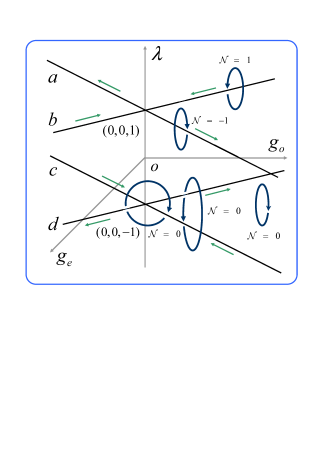
Figure 1: Schematic illustration of the degenerate lines and corresponding topological invariant in $3$-dimensional parameter space. There are four lines a, b, c, d, which cross at the $\lambda$ axis. The topological feature of the nodal lines is characterized by the path integral along the loops, as topological invariant, which is denoted for each loop. The obtained results indicate that the topological feature of the degenerate lines is equivalent to that of the magnetic fields produced by the current-carrying wires (a,b,c,d) with directions denoted by arrows.

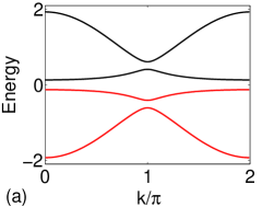
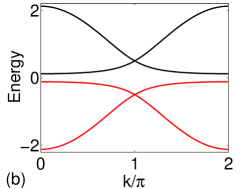
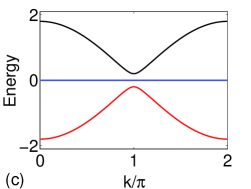
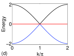
Figure 2: (Color online) Energy spectra from Eq. (8) at typical points (a) $g_{e}=0.5$, $g_{o}=0.5$, $\lambda=0.8;$ (b) $g_{e}=0.5$, $g_{o}=0.5$, $\lambda=1;$(c) $g_{e}=0$, $g_{o}=0$, $\lambda=0.8;$(d) $g_{e}=0$, $g_{o}=0$, $\lambda=1$. We see that (a) in general, there are four energy bands with symmetry about zero energy; (b) the two positive (negative) bands touch each other at a single point when $g_{e}=\pm g_{o}$; (c) when $g_{e}=g_{o}=0,$ two energy bands near the zero point become a flat band; (d) the top and the bottom bands touch each other at a single point at the flat band.

III Band structure and symmetry

Based on the solution of $h_{k}$, all the properties of the system can be obtained. Now we focus on the property of the eigenstates of $h_{k}$. We introduce a particle-hole transformation $\mathcal{P}$, which is defined as

$$\mathcal{P}^{-1}c_{l}\mathcal{P}=c_{l}^{\dagger}.$$ (15)

Applying $\mathcal{P}$ on operators $\alpha_{k}$ and $\beta_{k}$ we immediately have

$$\mathcal{P}^{-1}\alpha_{k}\mathcal{P}=\alpha_{-k}^{\dagger},\mathcal{P}^{-1}\beta_{k}\mathcal{P}=\beta_{-k}^{\dagger},$$ (16)

and

$$\mathcal{P}^{-1}\psi_{k}\mathcal{P}=C\psi_{k},$$ (17)

where

$$C=\left(\begin{array}[]{cccc}-1&0&0&0\\ 0&-1&0&0\\ 0&0&1&0\\ 0&0&0&1\end{array}\right).$$ (18)

It is easy to check that

$$\{C,h_{k}\}=0,$$ (19)

i.e., $h_{k}$ has the particle-hole symmetry. From the secular equation $h_{k}\left|\phi_{\rho\sigma}^{k}\right\rangle=\varepsilon_{\rho\sigma}^{k}\left|\phi_{\rho\sigma}^{k}\right\rangle$, we have

$$C\left|\phi_{\rho\sigma}^{k}\right\rangle=\left|\phi_{\bar{\rho}\sigma}^{k}\right\rangle,$$ (20)

with labels $\overline{\sigma}=-\sigma$ and $\overline{\rho}=-\rho$, which accords with the expression of $\left|\phi_{\rho\sigma}^{k}\right\rangle$ in Eq. (9). Then we have

$$\left\langle\phi_{\rho\sigma}^{k}\right|\partial_{k}\left|\phi_{\rho\sigma}^{k}\right\rangle=\left\langle\phi_{\bar{\rho}\sigma}^{k}\right|\partial_{k}\left|\phi_{\bar{\rho}\sigma}^{k}\right\rangle,$$ (21)

which indiates that the particle state $\left|\phi_{+\sigma}^{k}\right\rangle$ and hole state $\left|\phi_{-\sigma}^{k}\right\rangle$ have the identical Berry connection.

We note that $C$ and $h_{k}$ cannot have the common eigenstates. However, we have

$$[C,(h_{k})^{2}]=0,$$ (22)

which means that $C$ and $(h_{k})^{2}$ can have the same eigenstates. In other word, matrix $(h_{k})^{2}$ can be block diagonalized in the $\mathcal{P}$ symmetry invariant subspaces. Actually it is easy to check that

$$2(h_{k})^{2}=\left(\begin{array}[]{cc}h_{k}^{e}&0\\ 0&h_{k}^{o}\end{array}\right)+\Lambda_{k},$$ (23)

where

$$h_{k}^{e}=\left(\begin{array}[]{cc}\Lambda_{k}-2g_{e}^{2}&-2\gamma_{-k}g_{e}\\ -2\gamma_{k}g_{e}&2g_{e}^{2}-\Lambda_{k}\end{array}\right),$$ (24)

and

$$h_{k}^{o}=\left(\begin{array}[]{cc}\Lambda_{k}-2g_{o}^{2}&2\gamma_{k}g_{o}\\ 2\gamma_{-k}g_{o}&2g_{o}^{2}-\Lambda_{k}\end{array}\right).$$ (25)

Straightforward derivation shows that matrices $h_{k}^{e}$ and $h_{k}^{o}$ have the relations: (i)

$$\sigma_{y}h_{k}^{e}\sigma_{y}=-h_{-k}^{e},\sigma_{y}h_{k}^{o}\sigma_{y}=-h_{-k}^{o},$$ (26)

with

$$\sigma_{y}=\left(\begin{array}[]{cc}0&-i\\ i&0\end{array}\right);$$ (27)

(ii) they have the same eigenvalues

$$\epsilon_{\sigma}^{k}=2(\varepsilon_{\rho\sigma}^{k})^{2}-\Lambda_{k}.$$ (28)

It indicates that, the four bands can be reduced to two bands. For an arbitrary state in the form

$$\left|\Phi_{\sigma}^{k}\right\rangle=\alpha\left|\phi_{\sigma\sigma}^{k}\right\rangle+\beta|\phi_{\bar{\sigma}\sigma}^{k}\rangle,$$ (29)

we always have

$$\left[2(h_{k})^{2}-(g_{e}^{2}+g_{o}^{2}+|\gamma_{k}|^{2})\right]\left|\Phi_{\sigma}^{k}\right\rangle=\epsilon_{\sigma}^{k}\left|\Phi_{\sigma}^{k}\right\rangle.$$ (30)

Furthermore, applying operator

$$\Sigma=\left(\begin{array}[]{cc}\sigma_{y}&0\\ 0&-\sigma_{y}\end{array}\right),$$ (31)

on the Eq. (30), we have

$$\epsilon_{\bar{\sigma}}^{k}\Sigma\left|\Phi_{\sigma}^{k}\right\rangle = -\epsilon_{\sigma}^{k}\Sigma\left|\Phi_{\sigma}^{k}\right\rangle$$ (32)

$$= \left[2(h_{-k})^{2}-(g_{e}^{2}+g_{o}^{2}+|\gamma_{k}|^{2})\right]\Sigma\left|\Phi_{\sigma}^{k}\right\rangle.$$

Then we have

$$\Sigma\left|\Phi_{\sigma}^{k}\right\rangle=\alpha^{\prime}\left|\phi_{\bar{\sigma}\bar{\sigma}}^{-k}\right\rangle+\beta^{\prime}|\phi_{\sigma\bar{\sigma}}^{-k}\rangle=\left|\Phi_{\bar{\sigma}}^{\prime-k}\right\rangle,$$ (33)

which reveals the relation between $\left|\Phi_{\sigma}^{k}\right\rangle$ and the eigenstate $\left|\Phi_{\overline{\sigma}}^{\prime-k}\right\rangle$ of $(h_{-k})^{2}$. Here factors $\alpha^{\prime}$ and $\beta^{\prime}$ is obtained as $\alpha$ and $\beta$ from the expression of  in Eq. (29). We have another relation about the Berry connection

$$\left\langle\phi_{\rho\rho}^{k}\right|\partial_{k}\left|\phi_{\rho\rho}^{k}\right\rangle=\left\langle\phi_{\rho\bar{\rho}}^{-k}\right|\partial_{k}\left|\phi_{\rho\bar{\rho}}^{-k}\right\rangle.$$ (34)

These results are the basement for exploring the topological feature of the system.

In addition, two $2\times 2$ matrices $h_{k}^{e}$ and $h_{k}^{o}$ characterize the same physics of the $4\times 4$ matrix $h_{k}$ with a simpler form. For example, in the planes of $g_{o}=\pm g_{e}$, Eq. (28) is reduced to $\left|\lambda+e^{ik}\right|\sqrt{\left|\lambda+e^{ik}\right|^{2}+4g_{o}^{2}}$. According to the method developed in Ref. ZG PRL ; ZG1 ; LC1 , four nodal lines, are topological quantum-phase boundaries. Actually, such a dispersion relation links to a loop with parameter equation

$$\left\{\begin{array}[]{c}x=B_{0}(\lambda+\cos k)\\ y=B_{0}\sin k\end{array}\right.,$$ (35)

where $B_{0}=\sqrt{\lambda^{2}+2\lambda\cos k+1+4g_{o}^{2}}$. The winding number of the loop

$$v=\left\{\begin{array}[]{cc}1,&\left|\lambda\right|<1\\ 0,&\left|\lambda\right|>1\end{array}\right.,$$ (36)

which identify the topological invariants of the quantum phases.

IV Topological invariants

The aim of this paper is to investigate the topological feature of the nodal lines in the three dimensional parameter space. The topological properties of $1$D system are characterized by the so-called Zak phase, the Berry’s phase picked up by an eigenstate of $h_{k}$ sweeping across the Brillouin zone. There are four eigenstates for a given $k$. The Zak phase for the branch of $\left|\phi_{\rho\sigma}^{k}\right\rangle$ is

$$\mathcal{Z}_{\rho\sigma}(g_{e},g_{o},\lambda)=\frac{1}{2\pi}\int_{-\pi}^{\pi}\left\langle\phi_{\rho\sigma}^{k}\right|\frac{\partial}{\partial k}\left|\phi_{\rho\sigma}^{k}\right\rangle dk.$$ (37)

The equations of the Berry connection (21) and (34) show that

$$\mathcal{Z}_{\rho\sigma}=\mathcal{Z}_{\bar{\rho}\sigma},\mathcal{Z}_{\rho\rho}=-\mathcal{Z}_{\rho\bar{\rho}}$$ (38)

which allow us only consider the property of the Zak phase $\mathcal{Z}_{++}$. In the following we neglect the subscript by taking $\mathcal{Z}_{++}=\mathcal{Z}$.

It has been shown that quantity

$$\mathcal{N}=\oint_{L}\mathbf{\nabla}\mathcal{Z}\cdot d\mathbf{r},$$ (39)

is equivalent to Chern number, which is quantized as a topological invariant, characterizing the degenerate point in the parameter space. Here $\mathbf{\nabla}$ is the nabla operator

$$\mathbf{\nabla}=(\frac{\partial}{\partial g_{e}}\mathbf{i}+\frac{\partial}{\partial g_{o}}\mathbf{j}+\frac{\partial}{\partial\lambda}\mathbf{k}),$$ (40)

and $r=g_{e}i+g_{o}j+\lambda k$ is the vector in the parameter space. The value of $N$ depends on the topology of loop $L$ in the parameter space: $N$ is zero if the loop does not encircle the nodal line, while may be nonzero if encircle the nodal line. However, it is a little complicated to determine the exact integer $N$ from the direct derivation from state $\left|\phi_{\rho\sigma}^{k}\right\rangle$. Nevertheless, all the loops have the same $N$, if they encircle the identical nodal lines. Therefore, each of semi-infinite lines has their own field current, indicating the Chern number encircling them. In order to determine the Chern number, we rewrite $h_{k}$ as the form

$$h_{k}=\left(\begin{array}[]{cccc}2g_{o}&\gamma_{-k}&0&\gamma_{-k}\\ \gamma_{k}&2g_{{}_{e}}&-\gamma_{k}&0\\ 0&-\gamma_{-k}&-2g_{o}&-\gamma_{-k}\\ \gamma_{k}&0&-\gamma_{k}&-2g_{{}_{e}}\end{array}\right),$$ (41)

in the operator basis

$$\psi_{k}^{{\dagger}}=\frac{1}{\sqrt{2}}\left(\begin{array}[]{cccc}-\beta_{-k},&\alpha_{-k},&-\beta_{k}^{\dagger},&\alpha_{k}^{{\dagger}}\end{array}\right).$$ (42)

In the case of $g_{o}\approx g_{e}\gg 1\gg\left|1-\lambda\right|$, we have

$$h_{k}\approx\left(\begin{array}[]{cc}h_{k}^{\mathrm{RM}}&0\\ 0&-h_{k}^{\mathrm{RM}}\end{array}\right)+\left(g_{o}+g_{e}\right)\left(\begin{array}[]{cc}I_{2}&0\\ 0&-I_{2}\end{array}\right),$$ (43)

where the core matrix

$$h_{k}^{\mathrm{RM}}=\left(\begin{array}[]{cc}\Delta&\gamma_{-k}\\ \gamma_{k}&-\Delta\end{array}\right),$$ (44)

is nothing but the Bloch Hamiltonian of a standard RM model Rice , with a staggered on-site potential $\Delta=g_{o}-g_{e}$.

It has been shown that if the system adiabatically evolves along a loop enclosing the degeneracy points $(0,\pm 1)$ in the $\Delta-\lambda$ plane, then the polarization will be changed by $\pm 1$, where the sign depends on the direction of the loop. On the other hand, if the loop does not contain the degeneracy point, then the pumped charge is zero XD . Similarly, the direction of each nodal lines can be determined. We demonstrate topological properties of these lines in Fig. 1, which indicates that the nodal lines act as current carrying wires, obeying the topology of the electric circuits.

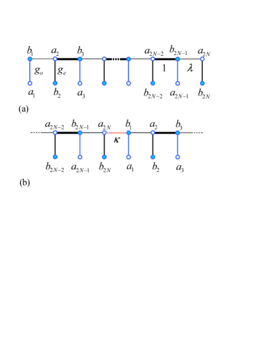
Figure 3: (Color online) Lattice geometries for the Majorana models described in Eqs. (V) and (65), with open boundary (a) and weak tunneling $\kappa$ between two ends (b), respectively. Solid (empty) circle indicates (anti) Majorana modes, while solid and dashed lines indicate intra-chain and across end to end weak hopping terms, respectively. Both panels (a) and (b) represent a SSH chain with staggered side-couplings, forming a comb-like lattice.

V Edge modes and adiabatic transport

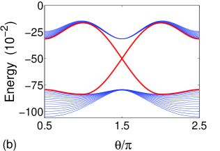
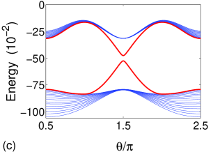
Figure 4: (Color online) (a) Majorana dimensionless center of mass distribution on the parameter space, $(g_{o}-g_{e})-\lambda$ plane for the mid-gap state in Eq. (64). There are four regions filled by different colors. If we calculate the change of $\eta$ along a loop enclosing the degeneracy point $(0,\pm 1)$ in the space, then $\eta$ will be changed by $\pm 1$. On the other hand, if the loop does not contain the degeneracy point, then the change of $\eta$ is zero. (b) and (c) are plots of the spectra of Majorana lattice with parameters along the cycle in (a) with open and weak link boundary condition respectively. The spectrum (c) indicates that the change of $\eta$ along a loop can be obtained by an adiabatic process for the mid-gap state marked in red.

The above results indicate that the quantum phase boundaries of the model $H$ exhibit the topological characterization. Inspired by the principle of bulk-edge correspondence we expect that the hidden topology behind the model can be unveiled by exploring the edge modes of the corresponding Majorana Hamiltonian. In general, the edge modes always live at zero energy J.A . However, the key feature as a topological invariant is the bound state, rather than the zero eigenvalue, which may be shifted by a constant for some specific model. We will see this point from the following example. Considering the spinless fermion system with an open boundary condition, the Hamiltonians read

$$H_{\mathrm{CH}}=H-M,$$

$$M=\left(c_{2N}^{\dagger}c_{1}^{\dagger}+c_{2N}^{\dagger}c_{1}\right)+\mathrm{H.c.},$$ (45)

which represent the original system with breaking the couplings across neighboring sites $(2N,1)$.

We introduce Majorana fermion operators

$$a_{j}=c_{j}^{\dagger}+c_{j},b_{j}=-i\left(c_{j}^{\dagger}-c_{j}\right),$$ (46)

which satisfy the relations

$$\left\{a_{j},a_{j^{\prime}}\right\} = 2\delta_{j,j^{\prime}},\left\{b_{j},b_{j^{\prime}}\right\}=2\delta_{j,j^{\prime}},$$

$$\left\{a_{j},b_{j^{\prime}}\right\} = 0,a_{j}^{2}=b_{j}^{2}=1.$$ (47)

The inverse transformation is

$$c_{j}^{\dagger}=\frac{1}{2}\left(a_{j}+ib_{j}\right),c_{j}=\frac{1}{2}\left(a_{j}-ib_{j}\right).$$ (48)

Then the Majorana representation of the Hamiltonian is

$$H_{\mathrm{CH}} = \sum\limits_{l=1}^{2N}\frac{i}{2}\left(\mu_{l}a_{l}b_{l}-\mathrm{H.c.}\right)$$ (49)

$$+\sum\limits_{l=1}^{N-1}\frac{i}{2}\left(\lambda b_{2l-1}a_{2l}+b_{2l+1}a_{2l}-\mathrm{H.c.}\right)$$

$$+\frac{i}{2}\left(\lambda b_{2N-1}a_{2N}-\mathrm{H.c.}\right),$$

where

$$\mu_{l}=\left\{\begin{array}[]{cc}g_{e},&\text{even }l\\ g_{o},&\text{odd }l\end{array}\right..$$ (50)

We write down the Hamiltonian in the basis $\varphi^{T}=(a_{1},$ $b_{1},$ $a_{2},$ $b_{2},$ $a_{3},$ $b_{3},$ $...)$ and see that

$$H_{\mathrm{CH}}=\varphi^{T}h_{\mathrm{CH}}\varphi,$$ (51)

where $h_{\mathrm{CH}}$ represents a $4N\times 4N$ matrix. Here matrix $h_{\mathrm{CH}}$ is explicitly written as

$$h_{\mathrm{CH}} = \frac{i}{2}\sum\limits_{l=1}^{2N}\left(\mu_{l}\left|l\right\rangle_{AB}\left\langle l\right|-\mathrm{H.c.}\right)$$

$$+\frac{i}{2}\sum\limits_{l=1}^{N-1}(\lambda\left|2l-1\right\rangle_{BA}\left\langle 2l\right|+\left|2l+1\right\rangle_{BA}\left\langle 2l\right|$$

$$-\mathrm{H.c.})+\frac{i}{2}(\lambda\left|2N-1\right\rangle_{BA}\left\langle 2N\right|-\mathrm{H.c.}),$$

where basis $\left\{\left|l\right\rangle_{A},\left|l\right\rangle_{B},l\in\left[1,2N\right]\right\}\$is an orthonormal complete set, ${}_{\alpha}\langle l\left|l^{\prime}\right\rangle_{\beta}=\delta_{ll^{\prime}}\delta_{\alpha\beta}$. The basis array is $(\left|1\right\rangle_{A},$ $\left|1\right\rangle_{B},$ $\left|2\right\rangle_{A},$ $\left|2\right\rangle_{B},$ $\left|3\right\rangle_{A},$ $\left|3\right\rangle_{B},$ $...)$, which accords with $\varphi^{T}$. Schematic illustrations for structures of $h_{\mathrm{CH}}$ are described in Fig. 3. It is expected to have another quantity which allows us to discern two kinds loops encircling a nodal line or not (also including different types of nodal lines). To this end, we introduce the concept of center of mass of Majorana fermion for a mid-gap state $\left|\chi_{\rho\sigma}\right\rangle$, which is defined as

$$\eta_{\rho\sigma}=\frac{1}{2N}\sum\limits_{l=1}^{2N}\left\langle\chi_{\rho\sigma}\right|l(\left|l\right\rangle_{AA}\left\langle l\right|+\left|l\right\rangle_{BB}\left\langle l\right|)\left|\chi_{\rho\sigma}\right\rangle.$$ (53)

Here we take dimensionless length, and then the range of $\eta_{\rho\sigma}$ is $[0,1]$. In the following, we will show that all the mid-gap states and the corresponding $\eta$ can be obtained exactly.

For $\left|\lambda\right|<1$ the mid-gap states $\left|\chi_{\rho\sigma}\right\rangle$ with eigenvalue $E_{\rho\sigma}$

$$\left(\begin{array}[]{c}\left|\chi_{++}\right\rangle\\ \left|\chi_{+-}\right\rangle\\ \left|\chi_{-+}\right\rangle\\ \left|\chi_{--}\right\rangle\end{array}\right) = \frac{1}{\Omega}\sum\limits_{l=1}^{N}\left(\begin{array}[]{c}\left(-\lambda\right)^{l-1}(\left|2l-1\right\rangle_{A}-i\left|2l-1\right\rangle_{B}),\\ \left(-\lambda\right)^{N-l}(\left|2l\right\rangle_{A}-i\left|2l\right\rangle_{B}),\\ \left(-\lambda\right)^{N-l}(\left|2l\right\rangle_{A}+i\left|2l\right\rangle_{B}),\\ \left(-\lambda\right)^{l-1}(\left|2l-1\right\rangle_{A}+i\left|2l-1\right\rangle_{B}),\end{array}\right),$$ (62)

$$2E_{\rho\sigma} = \left(g_{o},g_{e},-g_{e},-g_{o}\right),$$ (63)

where $\Omega=\sqrt{2\left(1-\lambda^{2N}\right)/\left(1-\lambda^{2}\right)}\approx\sqrt{2/\left(1-\lambda^{2}\right)}$. We note that they are all edged states but not zero mode. The corresponding center of mass are

$$\eta=\eta_{\rho\sigma}=\frac{1}{N\Omega^{2}}\sum\limits_{l=1}^{N}\left\{\begin{array}[]{cc}\left(2l-1\right)\lambda^{2\left(l-1\right)},&\rho-\sigma=0\\ \left(2l\right)\lambda^{2\left(N-l\right)},&\rho+\sigma=0\end{array}\right..$$ (64)

It shows that when $\left|\lambda\right|$ approaches to $1$, the mid-gap states close to extended states with a uniform probability distribution, the center of mass locate at the center of chain. And the level becomes the band edge in the region $\left|\lambda\right|\leqslant 1$. It accords with the plots of band structure of $h_{\mathrm{CH}}$ in Fig. 4.

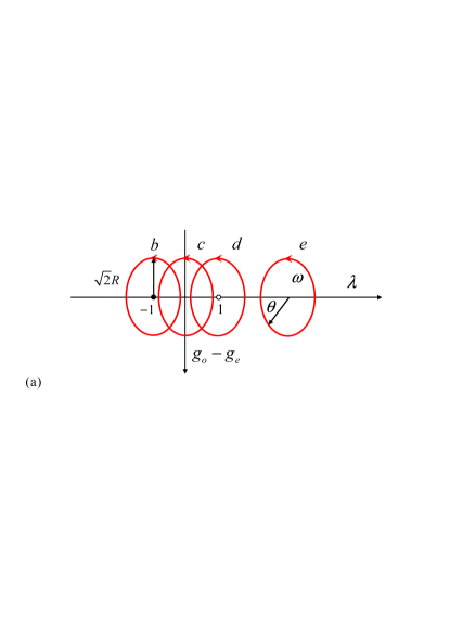
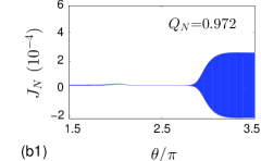
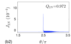
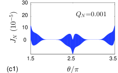
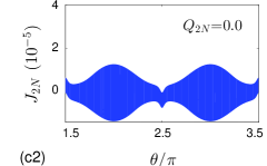
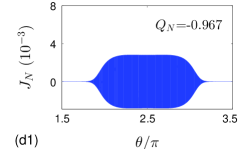
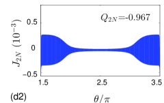
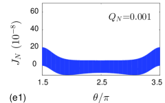
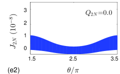
Figure 5: (Color online) (a) Schematics of four cycles around several typical points in the parameter space, $(g_{o}-g_{e})-\lambda$ plane. The radius $R=0.95$, points $b$ at $(0,-1)$ and $d$ at $(0,1)$ are two degeneracy points with opposite topological invariants, while points $c$ at $(0,0)$ and $e$ at $(0,4)$ are two trivial points. (b)-(e) are plots of Majorana current and the corresponding total probability transfer for quasi-adiabatic process. The results are obtained numerically for the system with $N=8$ and $\kappa=0.02$. The speed of time evolution is $\omega=5\times 10^{-7}$. It indicates that the topological invariant can be obtained by dynamical process.

If we only focus on the mid-gap state just under the first band (shown as red in Fig. 4(b)). It experiences a sudden change at the vicinity of $g_{e}=g_{o}$ in the region $\left|\lambda\right|\leqslant 1$. Accordingly, there is a jump from $0$ to $1$ for the center of mass. This behavior is familiar to that of polarization associated with the Zak’s phase XD . In general, the topological charge pumping is a transport of charge through an adiabatic cyclic evolution of the underlying Hamiltonian. The term topology originates from the fact that the transported charge is quantized and purely determined by the topology of the pump cycle, making it robust to perturbation. Furthermore, the pumped charge in each cycle can be connected to a topological invariant, the Chern number. In the present system, we consider the transport of Majorana fermion. If the system adiabatically evolves along a loop enclosing the degeneracy line in the $(g_{e},g_{o},\lambda)$ space, then the center of mass will be changed by $1$, which means that if we allow $(g_{e},g_{o},\lambda)$ to change in time along this loop, a quantized probability of Majorana fermion is pumped out of the system after one cycle. It is a similar idea with the Thouless topological pump D.J ; Y.H2 . On the other hand, if the loop does not contains the degeneracy lines, then the pumped probability is zero. The particle can be pumped out from the left or the right end of the system, which depends on the direction of the loop. In other word, the pumped Majorana fermion in each cycle can be connected to its winding number associated with the field P. To demonstrate this point, we plot the function $\eta(g_{e},g_{o},\lambda)$ in the $(g_{o}-g_{e})-\lambda$ plane Fig. 4(a). It is clearly that the degeneracy points act as the vortices of the field $\eta$.  It indicates that the transport of the Majorana center of mass directly connect to the topological invariant.

In practice, the pumped probability can be detected by a dynamical process in a ring system, where the two ends of the Majorana lattice is connected by a weak coupling. The Hamiltonian has the form

$$h_{\mathrm{R}}=h_{\mathrm{CH}}+\frac{i\kappa_{1,2N}}{2}(\left|1\right\rangle_{BA}\left\langle 2N\right|-\mathrm{H.c})$$ (65)

where $\kappa$ is the hopping constant of the weak tunneling. In the presence of $\kappa$, the spectrum of the Majorana lattice is changed, which allows the pumped probability flow along the ring. To illustrate this point, we plot the spectra of $h_{\mathrm{CH}}$ and $h_{\mathrm{R}}$ respectively for a circle around a degeneracy point in Fig. 4(b) and Fig. 4(c).

When we consider an adiabatic process for a mid-gap state, all the Majorana probability should pass through two neighboring site $(b_{n},a_{n+1})$ odd times if the adiabatic passage encloses a degeneracy line, otherwise even times. The transport of Majorana probability can be witnessed by the current across $(b_{n},a_{n+1})$, which is defined from the current operator

$$j_{n}=-\frac{\kappa_{n,n+1}}{2}\left\{\begin{array}[]{cc}(\left|n\right\rangle_{BA}\left\langle n+1\right|+\mathrm{H.c}),&n=2l-1\\ (\left|n\right\rangle_{AB}\left\langle n+1\right|+\mathrm{H.c}),&n=2l\end{array}\right.,$$ (66)

where $l=1,2,...,N$. The total pumped Majorana probability for an adiabatically evolved mig-gap state through a loop is

$$Q_{n}=\int_{0}^{T}J_{n}\mathrm{d}t,$$ (67)

where $J_{n}=\left\langle\Phi\left(t\right)\right|j_{n}\left|\Phi\left(t\right)\right\rangle$, $T$ is the period of the evolved time, satisfying $\left|\left\langle\Phi\left(t\right)\right|\Phi\left(t+T\right)\rangle\right|=1$ for any $t$. The topological invariant $\mathcal{N}$ for a given loop corresponds the dynamical quantity $Q_{n}$, which is independent of $n$. This is referred to dynamical bulk-edge correspondence, which links the topological feature in bulk to the dynamical quantity of the corresponding Majorana system.

To examine how the scheme works in practice, we simulate the quasi-adiabatic process by computing the time evolution numerically for finite system. We consider the dynamical process along circles in the parameter space, $(g_{o}-g_{e})-\lambda$ plane. The path equation is taken as the form

$$\left\{\begin{array}[]{c}g_{o}-g_{e}=\sqrt{2}R\cos(\omega t)\\ \lambda=\lambda_{\text{c}}+R\sin(\omega t)\end{array}\right.,$$ (68)

where $(0,\lambda_{\text{c}})$ and $R$ are the center and the semi-minor axis of the ellipse. For a given initial eigenstate $\left|\psi\left(0\right)\right\rangle$, the time evolved state is

$$\left|\Phi\left(t\right)\right\rangle=\exp(-i\int_{0}^{t}h_{\mathrm{R}}\left(t\right)\mathrm{d}t)\left|\psi\left(0\right)\right\rangle.$$ (69)

In low speed limit $\omega\rightarrow 0$, we have

$$f\left(t\right)=\left|\left\langle\Phi\left(t\right)\right|\psi\left(t\right)\rangle\right|\rightarrow 1,$$ (70)

where $\left|\psi\left(t\right)\right\rangle$ is the corresponding instantaneous eigenstate of $h_{\mathrm{R}}\left(t\right)$. The computation is performed by using a uniform mesh in the time discretization for the time-dependent Hamiltonian $H\left(t\right)$. In order to simulate a quasi-adiabatic process, we keep $f\left(t\right)>0.997$ for all the processes by taking sufficient small $\omega$. Fig. 5 plots the simulations of Majorana current and the corresponding total probability for several typical cases. It shows that the obtained dynamical quantities are in closer agreement with the expected values. This paves a way to detect the topological invariants by dynamical process.

We have established our main results, and a few comments are in order. First, notice that the zero mode states calculated here are not at exact zero-energy due to the finite-size of the system ($N=8$). Accordingly, the Majorana charges are not located at exact edges, i.e., the probability in the middle of the system is nonzero. However, the numerical results indicate that the character of topological pump is still evident. This is a benefit for experimental realization. Second, we would like to point out that the idea of the topological pump for ultracold atom has been realized experimentally S.Na ; M.L .

VI Summary

In conclusion, we have studied the topological feature of nodal lines in the dimerized Kitaev spin chain with a staggered transverse field. We have shown that the phase boundary line acts as a vortex filament associated with the field P generated by Zak phase. Unlike a topological quantum phase, which only corresponds to a point in parameter space, a topological nodal line always involves a loop in parameter space. In parallel, a nontrivial topological phase always associated with edge states in the open boundary, while a nontrivial loop is shown to be linked to a quantized charge pump. By Majorana transformation, we investigated a Thouless quantum pump with Majorana fermion analytically and numerically. Our results indicates that the quantized pumping charge can obtained by quasi-adiabatic circle evolution in a system with an impurity. It provides a way to observe the dynamical bulk-edge correspondence in experiment.

- (1) L. D. Landau, Phys. Z. Sowjetunion 11, 26 (1937).
- (2) V. L. Ginzburg and L. D. Landau, Zh. Eksp. Teor. Fiz. 20, 1064 (1950).
- (3) D. J. Thouless, M. Kohmoto, M. P. Nightingale, and M. den Nijs, Phys. Rev. Lett. 49, 405 (1982).
- (4) K. v. Klitzing, G. Dorda, and M. Pepper, Phys. Rev. Lett. 45, 494 (1980).
- (5) X. Chen, Z.-C. Gu, and X.-G. Wen, Phys. Rev. B 82, 155138 (2010).
- (6) R. B. Laughlin, Phys. Rev. Lett. 50, 1395 (1983).
- (7) V. Kalmeyer and R. B. Laughlin, Phys. Rev. Lett. 59, 2095 (1987).
- (8) N. Read and S. Sachdev, Phys. Rev. Lett. 66, 1773 (1991).
- (9) F. Pollmann, A. M. Turner, E. Berg, and M. Oshikawa, Phys. Rev. B 81, 064439 (2010).
- (10) X. Chen, Z.-C. Gu, and X.-G. Wen, Phys. Rev. B 84, 235128 (2011).
- (11) A. M. Turner, F. Pollmann, and E. Berg, Phys. Rev. B 83, 075102 (2011).
- (12) X.-G. Wen, Phys. Rev. B 85, 085103 (2012).
- (13) X. Chen, Z.-C. Gu, Z.-X. Liu, and X.-G. Wen, Science 338, 1604 (2012).
- (14) O. M. Sule, X. Chen, and S. Ryu, Phys. Rev. B 88, 075125 (2013).
- (15) Z.-C. Gu and M. Levin, Phys. Rev. B 89, 201113 (2014).
- (16) F. D. M. Haldane, Phys. Rev. Lett. 50, 1153 (1983).
- (17) C. L. Kane and E. J. Mele, Phys. Rev. Lett. 95, 146802 (2005).
- (18) C. L. Kane and E. J. Mele, Phys. Rev. Lett. 95, 226801 (2005).
- (19) B. A. Bernevig, T. L. Hughes, and S.-C. Zhang, Science 314, 1757 (2006).
- (20) M. Konig, S. Wiedmann, C. Brune, A. Roth, H. Buhmann, L. W. Molenkamp, X.-L. Qi, and S.-C. Zhan, Science 318, 766 (2007).
- (21) K. Nakada, M. Fujita, G. Dresselhaus, and M. S. Dresselhaus, Phys. Rev. B 54, 17954 (1996).
- (22) M. Fujita, K. Wakabayashi, K. Nakada, and K. Kusakabe, J. Phys. Soc. Jpn. 65, 1920 (1996).
- (23) A. H. Castro Neto, F. Guinea, N. M. R. Peres, K. S. Novoselov, and A. K. Geim, Rev. Mod. Phys. 81, 109 (2009).
- (24) Y. Niimi, T. Matsui, H. Kambara, K. Tagami, M. Tsukada, and H. Fukuyama, Appl. Surf. Sci. 241, 43 (2005).
- (25) Y. Kobayashi, K.-i. Fukui, T. Enoki, K. Kusakabe, and Y. Kaburagi, Phys. Rev. B 71, 193406 (2005).
- (26) Y. Niimi, T. Matsui, H. Kambara, K. Tagami, M. Tsukada, and H. Fukuyama, Phys. Rev. B 73, 085421 (2006).
- (27) G. E. Volovik, Jetp Lett. 93, 66 (2011).
- (28) Y. Tsutsumi, M. Ichioka, and K. Machida, Phys. Rev. B 83, 094510 (2011).
- (29) S. Murakami, New J. Phys. 9, 356 (2007).
- (30) X. Wan, A. M. Turner, A. Vishwanath, and S. Y. Savrasov, Phys. Rev. B 83, 205101 (2011).
- (31) G. Xu, H. Weng, Z. Wang, X. Dai, and Z. Fang, Phys. Rev. Lett. 107, 186806 (2011).
- (32) A. A. Burkov, and L. Balents, Phys. Rev. Lett. 107, 127205 (2011).
- (33) W. Witczak-Krempa and Y. B. Kim, Phys. Rev. B 85, 045124 (2012).
- (34) G. Chen and M. Hermele, Phys. Rev. B 86, 235129 (2012).
- (35) H.-J. Kim, K.-S. Kim, J.-F.Wang, M. Sasaki, N. Satoh, A. Ohnishi, M. Kitaura, M. Yang, and L. Li, Phys. Rev. Lett. 111, 246603 (2013).
- (36) P. Hosur and X. Qi, C. R. Phys. 14, 857 (2013).
- (37) T. Morimoto and A. Furusaki, Phys. Rev. B 89, 235127 (2014).
- (38) H. Weng, C. Fang, Z. Fang, B. A. Bernevig, and X. Dai, Phys. Rev. X 5, 011029 (2015).
- (39) J. Liu and D. Vanderbilt, Phys. Rev. B 90, 155316 (2014).
- (40) F. Wang and D.-H. Lee, Phys. Rev. B 86, 094512 (2012).
- (41) M. Sato, Phys. Rev. B 73, 214502 (2006).
- (42) B. Béri, Phys. Rev. B 81, 134515 (2010).
- (43) A. P. Schnyder and S. Ryu, Phys. Rev. B 84, 060504 (2011).
- (44) P. M. R. Brydon, A. P. Schnyder, and C. Timm, Phys. Rev. B 84, 020501 (2011).
- (45) A. P. Schnyder, P. M. R. Brydon, and C. Timm, Phys. Rev. B 85, 024522 (2012).
- (46) M. Sato, Y. Tanaka, K. Yada, and T. Yokoyama, Phys. Rev. B 83, 224511 (2011).
- (47) K. Yada, M. Sato, Y. Tanaka, and T. Yokoyama, Phys. Rev. B 83, 064505 (2011).
- (48) Y. Tanaka, Y. Mizuno, T. Yokoyama, K. Yada, and M. Sato, Phys. Rev. Lett. 105, 097002 (2010).
- (49) M. Sato and S. Fujimoto, Phys. Rev. Lett. 105, 217001 (2010).
- (50) S. Matsuura, P.-Y. Chang, A. P. Schnyder, and S. Ryu, New J. Phys. 15, 065001 (2013).
- (51) P.-Y. Chang, S. Matsuura, A. P. Schnyder, and S. Ryu, Phys. Rev. B 90, 174504 (2014).
- (52) X. Wan, A. M. Turner, A. Vishwanath, and S. Y. Savrasov, Phys. Rev. B 83, 205101 (2011).
- (53) K. Y. Yang, Y. M. Lu, and Y. Ran, Phys. Rev. B 84, 075129 (2011).
- (54) A. A. Burkov and L. Balents, Phys. Rev. Lett. 107, 127205 (2011).
- (55) G. Xu, H. Weng, Z. Wang, X. Dai, and Z. Fang, Phys. Rev. Lett. 107, 186806 (2011).
- (56) William Witczak-Krempa and Yong Baek Kim, Phys. Rev. B 85, 045124 (2012).
- (57) H. Weng, C. Fang, Z. Fang, B. A. Bernevig, and X. Dai, Phys. Rev. X 5, 011029 (2015).
- (58) S. M. Huang, et al. Nat. Commun. 6, 7373 (2015).
- (59) S. M. Young, et al. Phys. Rev. Lett. 108, 140405 (2012).
- (60) Z. Wang, et al. Phys. Rev. B 85, 195320 (2012).
- (61) Z. Wang, H. Weng, Q. Wu, X. Dai, and Z. Fang, Phys. Rev. B 88, 125427 (2013).
- (62) J. M. Hou, Phys. Rev. Lett. 111, 130403 (2013); J. M. Hou, Phys. Rev. B 89, 235405 (2014); J. M. Hou and W. Chen, Sci. Rep. 5, 17571 (2015); J. M. Hou and W. Chen, Sci. Rep. 6, 33512 (2016).
- (63) D. Sama, Nat. Phys. 8, 67–70 (2012).
- (64) Z. K. Liu, et al. Science 343, 864–867 (2014).
- (65) M. Neupane, et al. Nat. Commun. 5, 3786 (2014).
- (66) S. Y. Xu, et al. Science 349, 613–617 (2015).
- (67) B. Q. Lv, et al. Phys. Rev. X 5, 031013 (2015).
- (68) L. Lu, et al. Science 349, 622–624 (2015).
- (69) C. Li, S. Lin, G. Zhang, and Z. Song, Phys. Rev. B 96, 125418, (2017).
- (70) P. Wang, S. Lin, G. Zhang, and Z. Song, Sci. Rep. 7, 17179, (2017).
- (71) W. Chen, H.-Z. Lu, and J.-M. Hou, Phys. Rev. B 96, 041102 (2017).
- (72) Xiao-Qi Sun, Biao Lian, and Shou-Cheng Zhang, Phys. Rev. Lett. 119, 147001 (2017).
- (73) Y. Hatsugai, Phys. Rev. B 48, 11851 (1993).
- (74) A. Y. Kitaev, Phys. Usp. 44, 131 (2001).
- (75) S. Ryu and Y. Hatsugai, Phys. Rev. Lett. 89, 077002 (2002).
- (76) X.-L. Qi, Y.-S. Wu, and S.-C. Zhang, Phys. Rev. B 74, 045125 (2006).
- (77) Xiao-Yong Feng, Guang-Ming Zhang, and Tao Xiang, Phys. Rev. Lett. 98, 087204 (2007).
- (78) Xiaohui Wang, Tingting Liu, Ye Xiong, and Peiqing Tong, Phys. Rev. A 92, 012116 (2015).
- (79) Qi-Bo Zeng, Baogang Zhu, Shu Chen, L. You, and Rong Lü, Phys. Rev. A 94, 022119 (2016).
- (80) P. Jordan and E. Wigner, Z. Physik 47, 631 (1928).
- (81) A. Y. Kitaev, Phys. Usp. 44, 131 (2001).
- (82) Ning Wu, Physics Letters A 376, 3530–3534 (2012).
- (83) G. Zhang and Z. Song, Phys. Rev. Lett. 115, 177204 (2015).
- (84) G. Zhang, C. Li, and Z. Song, Sci. Rep. 7, 8176 (2017).
- (85) C. Li, G. Zhang, and Z. Song, Phy. Rev. A 94, 052113 (2016).
- (86) M. J. Rice, E. J. Mele, Phys. Rev. Lett. 49, 1455-1459 (1982).
- (87) Di Xiao, Ming-Che Chang, and Qian Niu, Rev. Mod. Phys. 82, 1959 (2010).
- (88) J. Alicea, Rep. Prog. Phys. 75, 076501 (2012).
- (89) D. J. Thouless, Phys. Rev. B 27, 6083 (1983).
- (90) Y. Hatsugai1,* and T. Fukui2, Phys. Rev. B 94, 041102(R) (2016).
- (91) S. Nakajima, T. Tomita, S. Taie, T. Ichinose, H. Ozawa, L.Wang, M. Troyer, and Y. Takahashi, Nat. Phys. 12, 296 (2016).
- (92) M. Lohse, C. Schweizer, O. Zilberberg, M. Aidelsburger, and I. Bloch, Nat. Phys. 12, 350 (2016).