Two-phase heat conductors with a surface
of the constant flow property

Lorenzo Cavallina , Rolando Magnanini , and Shigeru Sakaguchi11footnotemark: 1 Research Center for Pure and Applied Mathematics, Graduate School of Information Sciences, Tohoku University, Sendai, 980-8579, Japan (cava@ims.is.tohoku.ac.jp, sigersak@tohoku.ac.jp).Dipartimento di Matematica U. Dini, Università di Firenze, viale Morgagni 67/A, 50134 Firenze, Italy (rolando.magnanini@unifi.it).
Abstract

We consider a two-phase heat conductor in $\mathbb{R}^{N}$ with $N\geq 2$ consisting of a core and a shell with different constant conductivities. We study the role played by radial symmetry for overdetermined problems of elliptic and parabolic type.

First of all, with the aid of the implicit function theorem, we give a counterexample to radial symmetry for some two-phase elliptic overdetermined boundary value problems of Serrin-type.

Afterwards, we consider the following setting for a two-phase parabolic overdetermined problem. We suppose that, initially, the conductor has temperature 0 and, at all times, its boundary is kept at temperature 1. A hypersurface in the domain has the constant flow property if at every of its points the heat flux across surface only depends on time. It is shown that the structure of the conductor must be spherical, if either there is a surface of the constant flow property in the shell near the boundary or a connected component of the boundary of the heat conductor is a surface of the constant flow property. Also, by assuming that the medium outside the conductor has a possibly different conductivity, we consider a Cauchy problem in which the conductor has initial inside temperature 00 and outside temperature $1$. We then show that a quite similar symmetry result holds true.

Key words. heat equation, diffusion equation, two-phase heat conductor, transmission condition, initial-boundary value problem, Cauchy problem, constant flow property, overdetermined problem, symmetry.

AMS subject classifications. Primary 35K05 ; Secondary 35K10, 35B06, 35B40, 35K15, 35K20, 35J05, 35J25

1 Introduction

In this paper we examine several overdetermined elliptic and parabolic problems involving a two-phase heat conductor in ${\mathbb{R}}^{N}$, which consists of a core and a shell with different constant conductivities.

The study of overdetermined elliptic problems dates back to the seminal work of Serrin [Se], where he dealt with the so called torsion function, i.e. the solution to the following elliptic boundary value problem.

$$-\Delta u=1\;\text{in }\Omega,\quad u=0\;\text{ on }\partial\Omega.$$

Serrin showed that the normal derivative of the torsion function $u$ is a constant function on the boundary $\partial\Omega$ if and only if the domain $\Omega$ is a ball. We remark that such overdetermined conditions arise naturally in the context of critical shapes of shape functionals. In particular, if we define the torsional rigidity functional as $T(\Omega)=\int_{\Omega}u\,dx$, then Serrin’s overdetermination on the normal gradient of $u$ is equivalent to the shape derivative of $T$ vanishing for all volume preserving perturbations (we refer the interested reader to [HP, chapter 5]).

As far as overdetermined parabolic problems are concerned, we refer for example to [AG], where symmetry results analogous to Serrin’s one are proved as a consequence of an overdetermination on the normal derivative on the boundary, which is called the constant flow property in [Sav].

In this paper we show that two-phase overdetermined problems are inherently different. As a matter of fact, due to the introduction of a new degree of freedom (the geometry of the core $D$), we prove that two-phase elliptic overdetermined problems of Serrin-type admit non-symmetric solutions. On the other hand, we show that, for two-phase overdetermined problems of parabolic type, the stronger assumption of constant heat flow at the boundary for all time $t>0$ leads to radial symmetry (this result holds true even when the overdetermined condition is imposed only on a connected component of the boundary $\partial\Omega$). We will also examine another overdetermination, slightly different than the one introduced in [AG]. Namely we will consider the case where, instead of the boundary, the above mentioned constant flow property is satisfied on some fixed surface inside the heat conductor. We will show that, even in this case, the existence of such a surface satisfying the constant flow property leads to the radial symmetry of our heat conductor.

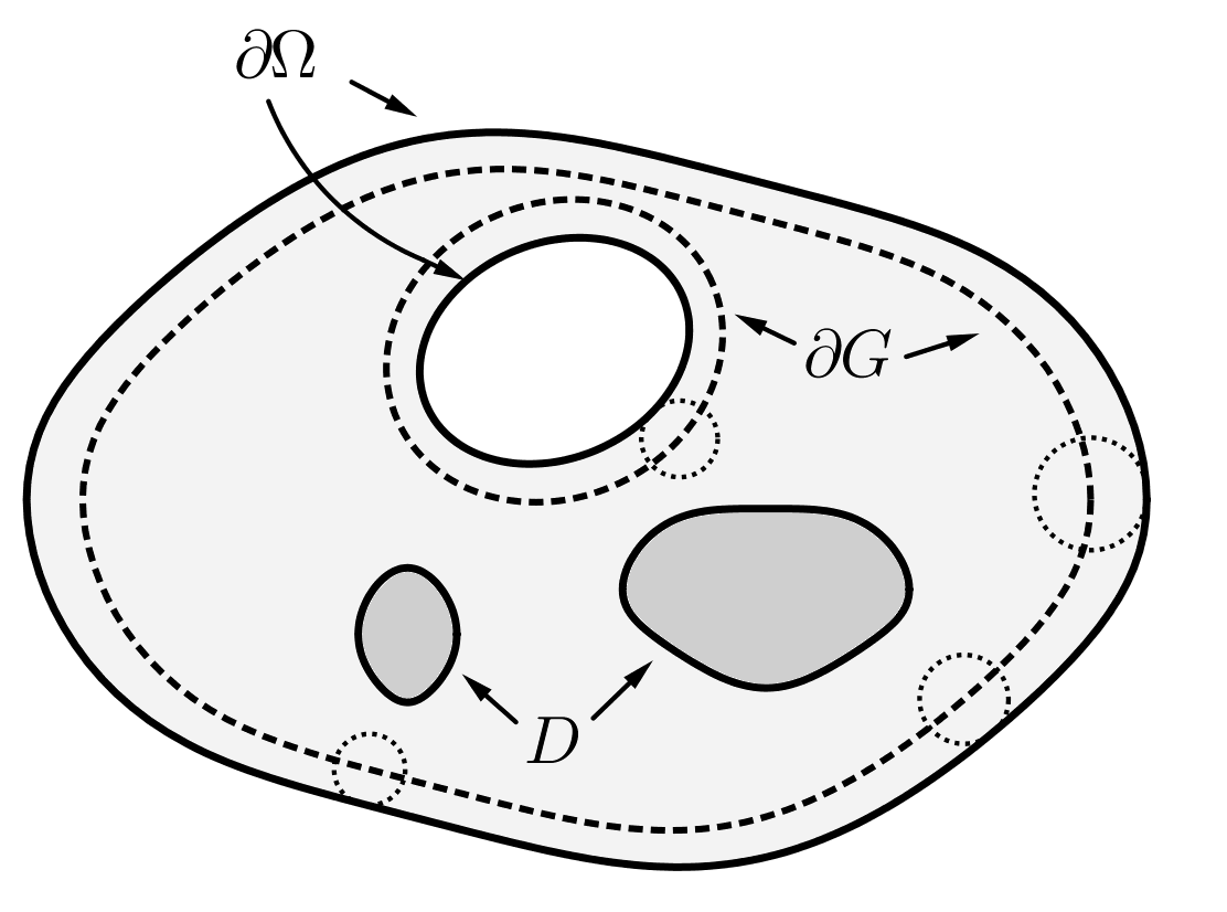
In what follows, we will introduce the notation and the main results of this paper. Let $\Omega$ be a bounded $C^{2}$ domain in $\mathbb{R}^{N}\ (N\geq 2)$ with boundary $\partial\Omega$, and let $D$ be a bounded $C^{2}$ open set in $\mathbb{R}^{N}$ which may have finitely many connected components. Assume that $\Omega\setminus\overline{D}$ is connected and $\overline{D}\subset\Omega$. Denote by $\sigma=\sigma(x)\ (x\in\mathbb{R}^{N})$ the conductivity distribution of the medium given by

$$\sigma=\begin{cases}\sigma_{c}\quad&\mbox{in }D,\\ \sigma_{s}\quad&\mbox{in }\Omega\setminus D,\\ \sigma_{m}\quad&\mbox{in }\mathbb{R}^{N}\setminus\Omega,\end{cases}$$

where $\sigma_{c},\sigma_{s},\sigma_{m}$ are positive constants and $\sigma_{c}\not=\sigma_{s}$. This kind of three-phase electrical conductor has been dealt with in [KLS] in the study of neutrally coated inclusions.

The first result is a counterexample to radial symmetry for the following two-phase elliptic overdetermined boundary value problems of Serrin-type:

$$\mbox{\rm div}(\sigma\nabla u)=\beta u-\gamma<0\ \mbox{ in }\Omega,\quad u=c\ \mbox{ and }\ \sigma_{s}\,\partial_{\nu}u=d_{0}\ \mbox{ on }\partial\Omega;$$ (1.1)

here, $\partial_{\nu}$ denotes the outward normal derivative at $\partial\Omega$, $\beta\geq 0$, $\gamma>0$, and $c\in\mathbb{R}$ are given numbers and $d_{0}$ is some negative constant determined by the data of the problem.

Theorem 1.1.

Let $B_{R}\subset B_{1}$ be concentric balls of radii $R$ and $1$. For every domain $\Omega$ of class $C^{2,\alpha}$ sufficiently close to $B_{1}$, there exists a domain $D$ of class $C^{2,\alpha}$ (and close to $B_{R}$) such that problem (1.1) admits a solution for the pair $(D,\Omega)$.

This result is an application of the implicit function theorem. It was shown by Serrin in [Se] that, in the one-phase case ($\sigma_{c}=\sigma_{s}$), a solution of (1.1) exists if and only if $\Omega$ is a ball. Thus, as we shall see for two-phase heat conductors, Theorem 1.1 sets an essential difference between the parabolic overdetermined regime in Theorem 1.4 and that in the elliptic problem (1.1).

A result similar to Theorem 1.1 appeared in [DEP], after we completed this paper. That result concerns certain semilinear equations (with a point-dependent nonlinearity) on compact Riemannian manifolds. The techniques used there do not seem to be easily applicable to the two-phase case.

The remaining part of this paper focuses on two-phase overdetermined problems of parabolic type. The papers [Sak1, Sak2] dealt with the heat diffusion over two-phase or three-phase heat conductors. Let $u=u(x,t)$ be the unique bounded solution of either the initial-boundary value problem for the diffusion equation:

$\displaystyle u_{t}=\mbox{ div}(\sigma\nabla u)\quad\mbox{ in }\ \Omega\times(0,+\infty),$ (1.2)
$\displaystyle u=1\ \quad\qquad\qquad\mbox{ on }\partial\Omega\times(0,+\infty),$ (1.3)
$\displaystyle u=0\ \quad\qquad\qquad\mbox{ on }\Omega\times\{0\},$ (1.4)

or the Cauchy problem for the diffusion equation:

$$u_{t}=\mbox{ div}(\sigma\nabla u)\quad\mbox{ in }\ \mathbb{R}^{N}\times(0,+\infty)\ \mbox{ and }\ u\ ={\mathcal{X}}_{\Omega^{c}}\ \mbox{ on }\mathbb{R}^{N}\times\{0\},$$ (1.5)

where ${\mathcal{X}}_{\Omega^{c}}$ denotes the characteristic function of the set $\Omega^{c}=\mathbb{R}^{N}\setminus\Omega$. Consider a bounded domain $G$ in $\mathbb{R}^{N}$ satisfying

$$\overline{D}\subset G\subset\overline{G}\subset\Omega\ \mbox{ and }\mbox{ dist}(x,\partial\Omega)\leq\mbox{ dist}(x,\overline{D})\ \mbox{ for every }x\in\partial G.$$ (1.6)
Refer to caption
Figure 1: The two-phase conductor described by $\Omega$ and $D$ and the surface $\partial G$.

In [Sak1, Sak2], the third author obtained the following theorems.

Theorem A ([Sak1]).

Let $u$ be the solution of problem (1.2)–(1.4), and let $\Gamma$ be a connected component of $\partial G$ satisfying

$$\mbox{\rm dist}(\Gamma,\partial\Omega)=\mbox{\rm dist}(\partial G,\partial\Omega).$$ (1.7)

If there exists a function $a\mathrel{\mathop{\mathchar 58\relax}}(0,+\infty)\to(0,+\infty)$ satisfying

$$u(x,t)=a(t)\ \mbox{ for every }(x,t)\in\Gamma\times(0,+\infty),$$ (1.8)

then $\Omega$ and $D$ must be concentric balls.

Theorem B ([Sak1, Sak2]).

Let $u$ be the solution of problem (1.5). Then the following assertions hold:

  • (a)

    if there exists a function $a\mathrel{\mathop{\mathchar 58\relax}}(0,+\infty)\to(0,+\infty)$ satisfying

    $$u(x,t)=a(t)\ \mbox{ for every }(x,t)\in\partial G\times(0,+\infty),$$ (1.9)

    then $\Omega$ and $D$ must be concentric balls;

  • (b)

    if $\sigma_{s}=\sigma_{m}$ and (1.8) holds on some connected component $\Gamma$ of $\partial G$ satisfying (1.7) for some function $a\mathrel{\mathop{\mathchar 58\relax}}(0,+\infty)\to(0,+\infty)$, then $\Omega$ and $D$ must be concentric balls.

The condition (1.8) (or (1.9)) means that $\Gamma$ (or $\partial G$) is an isothermic surface of the normalized temperature $u$ at every time; for this reason, $\Gamma$ (or $\partial G$) is called a stationary isothermic surface of $u$.

In this paper, we shall suppose that the solution $u$ of (1.2)–(1.4) or (1.5) admits a surface $\Gamma\subset{\overline{\Omega}}\setminus{\overline{D}}$ of the constant flow property, that is there exists a function $d\mathrel{\mathop{\mathchar 58\relax}}(0,+\infty)\to\mathbb{R}$ satisfying

$$\sigma_{s}\,\partial_{\nu}u(x,t)=d(t)\ \mbox{ for every }(x,t)\in\Gamma\times(0,+\infty),$$ (1.10)

where $\partial_{\nu}u$ denotes the outward normal derivative of $u$ at points in $\Gamma$.

We will then prove two types of symmetry results. We shall first start with symmetry theorems for solutions that admit a surface $\Gamma$ of the constant flow property in the shell $\Omega\setminus\overline{D}$ of the conductor.

Theorem 1.2.

Let $u$ be the solution of either problem (1.2)–(1.4) or problem (1.5), and let $\Gamma$ be a connected component of class $C^{2}$ of $\partial G$ satisfying (1.7).

If there exists a function $d\mathrel{\mathop{\mathchar 58\relax}}(0,+\infty)\to\mathbb{R}$ satisfying (1.10), then $\Omega$ and $D$ must be concentric balls.

With the aid of a simple observation on the initial behavior of the solution $u$ of problem (1.5)(see Proposition E) as in the proof of Theorem 1.2 for problem (1.5)(see Subsection 4.3), Theorems A and B combine to make a single theorem.

Theorem 1.3.

Let $u$ be the solution of either problem (1.2)–(1.4) or problem (1.5), and let $\Gamma$ be a connected component of $\partial G$ satisfying (1.7).

If there exists a function a:(0,+)(0,+):𝑎00a\mathrel{\mathop{\mathchar 58\relax}}(0,+\infty)\to(0,+\infty) satisfying (1.8), then ΩΩ\Omega and D𝐷D must be concentric balls.

A second kind of result concerns multi-phase heat conductors where a connected component of $\partial\Omega$ is a surface of the constant flow property or a stationary isothermic surface. We obtain three symmetry theorems, one for the Cauchy-Dirichlet problem (Theorem 1.4) and two for the Cauchy problem (Theorems 1.5 and 1.6), with different regularity assumptions.

Theorem 1.4.

Let $u$ be the solution of problem (1.2)–(1.4), and let $\Gamma$ be a connected component of $\partial\Omega$. Suppose that $\Gamma$ is of class $C^{6}$.

If there exists a function $d\mathrel{\mathop{\mathchar 58\relax}}(0,+\infty)\to\mathbb{R}$ satisfying (1.10), then $\Omega$ and $D$ must be concentric balls.

When $D=\varnothing$, $\Gamma=\partial\Omega$ and $\sigma$ is constant on $\mathbb{R}^{N}$, the same overdetermined boundary condition of Theorem 1.4 has been introduced in [AG, GS] and similar symmetry theorems have been proved by the method of moving planes introduced by [Se] and [Al]. Theorem 1.4 gives a new symmetry result for two-phase heat conductors, in which that method cannot be applied. Recently, an analogous problem was re-considered in [Sav] in the context of the heat flow in smooth Riemannian manifolds: it was shown that the same overdetermined boundary condition implies that $\partial\Omega$ must be an isoparametric surface (and hence $\partial\Omega$ is a sphere if compactness is assumed). We remark that the methods introduced in [Sav] cannot be directly applied to our two-phase setting due to a lack of regularity.

Theorem 1.5.

Let $u$ be the solution of problem (1.5), and let $\Gamma$ be a connected component of $\partial\Omega$. Suppose that $\Gamma$ is of class $C^{6}$.

If there exists a function a:(0,+)(0,+):𝑎00a\mathrel{\mathop{\mathchar 58\relax}}(0,+\infty)\to(0,+\infty) satisfying (1.8), then ΩΩ\Omega and D𝐷D must be concentric balls.

The $C^{6}$-regularity assumption of Theorems 1.4 and 1.5 does not seem very optimal, but it is needed to construct the barriers where we use the fourth derivatives of the distance function to the boundary. It can instead be removed for problem (1.5), in the particular the case in which $\sigma_{s}=\sigma_{m}$. This can be done by complementing the proof of Theorem 1.4 with the techniques developed in [MPS].

Theorem 1.6.

Set $\sigma_{s}=\sigma_{m}$ and let $u$ be the solution of problem (1.5). Let $\Gamma$ be a connected component of $\partial\Omega$.

  • (a)

    If there exists a function a:(0,+)(0,+):𝑎00a\mathrel{\mathop{\mathchar 58\relax}}(0,+\infty)\to(0,+\infty) satisfying (1.8), then ΩΩ\Omega and D𝐷D must be concentric balls.

  • (b)

    If $N\geq 3$, suppose that $\Gamma$ is strictly convex. If there exists a function $d\mathrel{\mathop{\mathchar 58\relax}}(0,+\infty)\to\mathbb{R}$ satisfying (1.10), then $\Omega$ and $D$ must be concentric balls.

The rest of the paper is organized as follows. Section 2 is devoted to the proof of Theorem 1.1, which is a combination of the implicit function theorem and techniques pertaining to the realm of shape optimization. In Section 3 we give some preliminary notations and recall some useful results from [Sak1, Sak2]. In Section 4, we shall carry out the proofs of Theorems 1.2 and 1.3, based on a balance law, the short-time behaviour of the solution, and on the study of a related elliptic problem. The proof of Theorem 1.4 will be performed in Section 5: the relevant parabolic problem will be converted into a family of elliptic ones, by a Laplace transform, and new suitable barriers controlled by geometric parameters of the conductor will be constructed for the transformed problem. The same techniques will also be used in Subsection 5.5 to prove Theorem 1.5. Section 6 contains the proof of Theorem 1.6: here, due to the more favorable structure of the Cauchy problem in hand, we are able to use the techniques of [MPS] to obtain geometrical information.

2 Non-uniqueness for a two-phase Serrin’s problem

Here, the proof of Theorem 1.1 will be obtained by a perturbation argument.

Let $D$, $\Omega\subset{\mathbb{R}}^{N}$ be two bounded domains of class $C^{2,\alpha}$ with $\overline{D}\subset\Omega$. We look for a pair $(D,\Omega)$ for which the overdetermined problem (1.1) has a solution for some negative constant $d_{0}$. By evident normalizations, it is sufficient to examine (1.1) with $\sigma_{s}=1$ in the form

$\displaystyle\mathop{\mathrm{div}}(\sigma\nabla u)=\beta u-\gamma<0\quad\mbox{ in }\ \Omega,$ (2.1)
$\displaystyle u=0\ \quad\qquad\qquad\qquad\qquad\mbox{ on }\partial\Omega,$ (2.2)
$\displaystyle\partial_{\nu}u=-\Lambda\ \quad\qquad\qquad\qquad\mbox{ on }\partial\Omega,$ (2.3)

where $\beta\geq 0$, $\gamma>0$, and $\sigma=\sigma_{c}{\mathcal{X}}_{D}+{\mathcal{X}}_{\Omega\setminus D}$. By the divergence theorem, the constant $\Lambda$ is related to the other data of the problem by the formula:

$$\Lambda=\frac{1}{|\partial\Omega|}\left\{\gamma\,|\Omega|-\beta\,\int_{\Omega}u\,dx\right\};$$ (2.4)

here, the bars indifferently denote the volume of $\Omega$ and the $(N-1)$-dimensional Hausdorff measure of $\partial\Omega$.

It is obvious that, for all values of $\sigma_{c}>0$, the pair $(B_{R},B_{1})$ in the assumptions of the theorem is a solution to the overdetermined problem (2.1)–(2.3) for some $\Lambda$. We will look for other solution pairs of (2.1)–(2.3) near $(B_{R},B_{1})$ by a perturbation argument which is based on the following version of the implicit function theorem, for the proof of which we refer to [N, Theorem 2.7.2, pp. 34–36].

Theorem C (Implicit function theorem).

Suppose that $\mathcal{F}$, $\mathcal{G}$ and $\mathcal{H}$ are three Banach spaces, $U$ is an open subset of $\mathcal{F}\times\mathcal{G}$, $(f_{0},g_{0})\in U$, and $\Psi\mathrel{\mathop{\mathchar 58\relax}}U\to\mathcal{H}$ is a Fréchet differentiable mapping such that $\Psi(f_{0},g_{0})=0$. Assume that the partial derivative $\partial_{f}\Psi(f_{0},g_{0})$ of $\Psi$ with respect to $f$ at $(f_{0},g_{0})$ is a bounded invertible linear transformation from $\mathcal{F}$ to ${\mathcal{H}}$.

Then there exists an open neighborhood $U_{0}$ of $g_{0}$ in $\mathcal{G}$ such that there exists a unique Fréchet differentiable function $f\mathrel{\mathop{\mathchar 58\relax}}U_{0}\to\mathcal{F}$ such that $f(g_{0})=f_{0}$, $(f(g),g)\in U$ and $\Psi(f(g),g)=0$ for all $g\in U_{0}$.

2.1 Preliminaries

We introduce the functional setting for the proof of Theorem 1.1. Set $D=B_{R}$ and $\Omega=B_{1}$. For $\alpha\in(0,1)$, let $\phi\in C^{2,\alpha}({\mathbb{R}}^{N},{\mathbb{R}}^{N})$ satisfy that $\mathrm{Id}+\phi$ is a diffeomorphism from ${\mathbb{R}}^{N}$ to ${\mathbb{R}}^{N}$, and

$$\phi=f\,\nu\ \mbox{ on }\ \partial D\quad\mbox{ and }\quad\phi=g\,\nu\ \mbox{ on }\ \partial\Omega,$$

where $\mathrm{Id}$ denotes the identity mapping, $f$ and $g$ are given functions of class $C^{2,\alpha}$ on $\partial D$ and $\partial\Omega$, respectively, and $\nu$ indistinctly denotes the outward unit normal to both $\partial D$ and $\partial\Omega$. Next, we define the sets

$$\Omega_{g}=(\mathrm{Id}+\phi)(\Omega)\ \mbox{ and }\ D_{f}=(\mathrm{Id}+\phi)(D).$$

If $f$ and $g$ are sufficiently small, $D_{f}$ and $\Omega_{g}$ are such that $\overline{D_{f}}\subset\Omega_{g}$.

Now, we consider the Banach spaces (equipped with their standard norms):

$\displaystyle\mathcal{F}=\Bigl{\{}f\in C^{2,\alpha}(\partial D)\mathrel{\mathop{\mathchar 58\relax}}\int_{\partial D}f\,dS=0\Bigr{\}},\quad{\mathcal{G}}=\Bigl{\{}g\in C^{2,\alpha}(\partial\Omega)\mathrel{\mathop{\mathchar 58\relax}}\int_{\partial\Omega}g\,dS=0\Bigr{\}},$
$\displaystyle{\mathcal{H}}=\Bigl{\{}h\in C^{1,\alpha}(\partial\Omega)\mathrel{\mathop{\mathchar 58\relax}}\int_{\partial\Omega}h\,dS=0\Bigr{\}}.$

In order to be able to use Theorem C, we introduce a mapping $\Psi\mathrel{\mathop{\mathchar 58\relax}}\mathcal{F}\times{\mathcal{G}}\to{\mathcal{H}}$ by:

$$\Psi(f,g)=\left\{\partial_{\nu_{g}}u_{f,g}+\Lambda_{f,g}\right\}J_{\tau}({g})\ \mbox{ for }\ (f,g)\in\mathcal{F}\times{\mathcal{G}}.$$ (2.5)

Here, $u_{f,g}$ is the solution of (2.1)–(2.2) with $\Omega=\Omega_{g}$ and $\sigma=\sigma_{c}\,\mathcal{X}_{D_{f}}+\mathcal{X}_{\Omega_{g}\setminus D_{f}}$, $\nu_{g}$ stands for the outward unit normal to $\partial\Omega_{g}$, and $\Lambda_{f,g}$ is computed via (2.4), with $\Omega=\Omega_{g}$ and $u=u_{f,g}$. Also, by a slight abuse of notation, $\partial_{\nu_{g}}u_{f,g}$ means the function of value

$$\nabla u_{f,g}(x+g(x)\,\nu(x))\cdot\nu_{g}(x+g(x)\,\nu(x))\ \mbox{ at any }x\in\partial\Omega,$$

where $\nu$ is the outward unit normal to $\partial\Omega$. Finally, the term $J_{\tau}(g)>0$ is the tangential Jacobian associated to the transformation $x\mapsto x+g(x)\,\nu(x)$ (see [HP, Definition 5.4.2, p. 190]): this term ensures that the image $\Psi(f,g)$ has zero integral over $\partial\Omega$ for all $(f,g)\in\mathcal{F}\times{\mathcal{G}}$, as an integration of (2.3) on $\partial\Omega_{g}$ requires, when $\Lambda=\Lambda_{f,g}$.

Thus, by definition, we have $\Psi(f,g)=0$ if and only if the pair $(D_{f},\Omega_{g})$ solves (2.1)–(2.3). Moreover, we know that the mapping $\Psi$ vanishes at $(f_{0},g_{0})=(0,0)$.

2.2 Computing the derivative of $\Psi$

The Fréchet differentiability of $\Psi$ in a neighborhood of $(0,0)\in\mathcal{F}\times\mathcal{G}$ can be proved, in a standard way, by following the proof of [HP, Theorem 5.3.2, pp. 183–184], with the help of the regularity theory for elliptic operators with piecewise constant coefficients. In particular, the Hölder continuity of the first and second derivatives of the function $u_{f,g}$ up to the interface $\partial D_{f}$, which is stated in [LU, Theorem 16.2, p. 222], is obtained by flattening the interface with a diffeomorphism of class $C^{2,\alpha}$ as in [LU, Chapter 4, Section 16, pp. 205–223] or in [DEF, Appendix, pp. 894–900] and by using the classical regularity theory for linear elliptic partial differential equations ([LU, Gi, ACM]).

We will now proceed to the actual computation of $\partial_{f}\Psi(0,0)$. Since $\Psi$ is Fréchet differentiable, $\partial_{f}\Psi(0,0)$ can be computed as a Gâteaux derivative:

$$\partial_{f}\Psi(0,0)(f)=\lim_{t\to 0}\frac{\Psi(tf,0)-\Psi(0,0)}{t}\ \mbox{ for }\ f\in\mathcal{F}.$$

From now on, we fix $f\in\mathcal{F}$, set $g=0$ and, to simplify notations, we will write $D_{t},u_{t},\Lambda(t)$ in place of $D_{tf},u_{tf,0},\Lambda_{tf,0}$; in this way, we can agree that $D_{0}=D$, $u_{0}=u$, and so on. Also, in order to carry out our computations, we introduce some standard notations, in accordance with [HP] and [DZ]: the shape derivative of $u$ is defined by

$$u^{\prime}(x)={\left.\kern-1.2pt\frac{d}{dt}\vphantom{|}\right|_{t=0}}u_{t}(x)\ \text{ for }\ x\in\Omega.$$ (2.6)

In particular, we will employ the use of the following characterization of the shape derivative $u^{\prime}$ of $u$. We refer to [Ca, Proposition 2.3] where the case $\beta=0$ is analyzed, and to [DK, Theorem 2.5] where $\beta<0$ is an eigenvalue. The case $\beta>0$ can be treated analogously and therefore the proof will be omitted.

Lemma 2.1.

For every $f\in\mathcal{F}$, the shape derivative $u^{\prime}$ of $u_{t}$ solves the following:

$\displaystyle\sigma\Delta u^{\prime}=\beta u^{\prime}$  $\displaystyle\quad\mbox{ in }\ D\cup(\Omega\setminus\overline{D}),$ (2.7)
$\displaystyle[\sigma\partial_{\nu}u^{\prime}]=0$  $\displaystyle\quad\mbox{ on }\partial D,$ (2.8)
$\displaystyle[u^{\prime}]=-[\partial_{\nu}u]f$  $\displaystyle\quad\mbox{ on }\partial D,$ (2.9)
$\displaystyle u^{\prime}=0$  $\displaystyle\quad\mbox{ on }\ \partial\Omega.$ (2.10)

In the above, we used square brackets to denote the jump of a function across the interface $\partial D$. More precisely, for any function $\varphi$ we mean $[\varphi]=\varphi_{+}-\varphi_{-}$, where the subscripts $+$ and $-$ denote the relevant quantities in the two phases $\Omega\setminus\overline{D}$ and $D$ respectively and the equality here is understood in the classical sense.

Lemma 2.2.

For all $f\in\mathcal{F}$ we have $\Lambda^{\prime}(0)=0$.

Proof.

We rewrite (2.4) as

$$\Lambda(t)|\partial\Omega|-\gamma|\Omega|=-\beta\int_{\Omega}u_{t}\,dS,$$

then differentiate and evaluate at $t=0$. The derivative of the left-hand side equals $\Lambda^{\prime}(0)\,|\partial\Omega|$. Thus, we are left to prove that the derivative of the function defined by

$$I(t)=\int_{\Omega}u_{t}\,dx$$

is zero at $t=0$.

To this aim, since $u_{t}$ solves (2.1) for $D=D_{t}$, we multiply both sides of this for $u_{t}$ and integrate to obtain that

$$\gamma\,I(t)=\gamma\int_{\Omega}u_{t}\,dx=\beta\int_{\Omega}u_{t}^{2}\,dx+\sigma_{c}\int_{D_{t}}\,\mathinner{\!\left\lvert\nabla u_{t}\,\right\rvert}^{2}dx+\int_{\Omega\setminus\overline{D_{t}}}\mathinner{\!\left\lvert\nabla u_{t}\,\right\rvert}^{2}dx,$$

after an integration by parts. Thus, the desired derivative can be computed by using Hadamard’s formula (see [HP, Corollary 5.2.8, p. 176]):

$\displaystyle\gamma\,I^{\prime}(0)$ $\displaystyle=2\beta\int_{\Omega}uu^{\prime}\,dx+2\int_{\Omega}\sigma\nabla u\cdot\nabla u^{\prime}\,dx+\sigma_{c}\int_{\partial D}(\partial_{\nu}u_{-})^{2}f\,dS-\int_{\partial D}(\partial_{\nu}u_{+})^{2}f\,dS$
$\displaystyle=2\beta\int_{\Omega}uu^{\prime}\,dx+2\int_{\Omega}\sigma\nabla u\cdot\nabla u^{\prime}\,dx=0.$

Here, in the second equality we used that $\partial_{\nu}u_{-}$ and $\partial_{\nu}u_{+}$ are constant on $\partial D$ and that $f\in\mathcal{F}$, while, the third equality ensues by integrating (2.7) against $u$. ∎

Theorem 2.3.

The Fréchet derivative $\partial_{f}\Psi(0,0)$ defines a mapping from $\mathcal{F}$ to ${\mathcal{H}}$ by the formula

$$\partial_{f}\Psi(0,0)(f)=\partial_{\nu}u^{\prime},$$

where $u^{\prime}$ is the solution of the boundary value problem (2.7)–(2.10).

Proof.

Since $\Psi$ is Fréchet differentiable, we can compute $\partial_{f}\Psi$ as a Gâteaux derivative as follows:

$$\partial_{f}\Psi(0,0)(f)={\left.\kern-1.2pt\frac{d}{dt}\vphantom{|}\right|_{t=0}}\Psi(tf,0)={\left.\kern-1.2pt\frac{d}{dt}\vphantom{|}\right|_{t=0}}\left\{\nabla u_{t}(x)\cdot\nu(x)+\Lambda(t)\right\}J_{\tau}(0).$$

Since $J_{\tau}(0)=1$, the thesis is a direct consequence of Lemma 2.2 and definition (2.6). Finally, the fact that this mapping is well-defined (i.e. $\partial_{\nu}u^{\prime}$ actually belongs to $\mathcal{H}$ for all $f\in\mathcal{F}$) follows from the calculation

$$\int_{\partial\Omega}\partial_{\nu}u^{\prime}\,dS=\int_{\Omega}\mathop{\mathrm{div}}(\sigma\nabla u^{\prime})\,dx=\beta\int_{\Omega}u^{\prime}\,dx=\beta\,I^{\prime}(0)=0,$$

where we also used (2.7)–(2.10). ∎

2.3 Applying the implicit function theorem

The following result clearly implies Theorem 1.1.

Theorem 2.4.

There exists $\varepsilon>0$ such that, for all $g\in\mathcal{G}$ with $\mathinner{\!\left\lVert g\right\rVert}<\varepsilon$ there exists a unique $f(g)\in\mathcal{F}$ such that the pair $(D_{f(g)},\Omega_{g})$ is a solution of the overdetermined problem (2.1)–(2.3).

Proof.

This theorem consists of a direct application of Theorem C. We know that the mapping $(f,g)\mapsto\Psi(f,g)$ is Fréchet differentiable and we computed its Fréchet derivative with respect to the variable $f$ in Theorem 2.3. We are left to prove that the mapping $\partial_{f}\Psi(0,0)\mathrel{\mathop{\mathchar 58\relax}}\mathcal{F}\to{\mathcal{H}}$, given in Theorem 2.3, is a bounded and invertible linear transformation.

Linearity and boundedness of $\partial_{f}\Psi(0,0)$ ensue from the properties of problem (2.7)–(2.10).

We are now going to prove the invertibility of $\partial_{f}\Psi(0,0)$. To this end we study the relationship between the spherical harmonic expansions of the functions $f$ and $u^{\prime}$ (we refer to [Ca, Section 4] where the same technique has been exposed in detail). Suppose that, for some real coefficients $\alpha_{k,i}$ the following holds

$$f(R\theta)=\sum_{k=1}^{\infty}\sum_{i=1}^{d_{k}}\alpha_{k,i}Y_{k,i}(\theta),\quad\mbox{ for }\theta\in\mathbb{S}^{N-1}.$$ (2.11)

Here $Y_{k,i}$ denotes the solution of the eigenvalue problem $-\Delta_{\mathbb{S}^{N-1}}Y_{k,i}=\lambda_{k}Y_{k,i}$ on $\mathbb{S}^{N-1}$, with $k$-th eigenvalue $\lambda_{k}=k(N+k-2)$ of multiplicity $d_{k}$. Under the assumption (2.11), we can apply the method of separation of variables to get

$$u^{\prime}(r\theta)=\sum_{k=1}^{\infty}\sum_{i=1}^{d_{k}}\alpha_{k,i}s_{k}(r)Y_{k,i}(\theta),\quad\mbox{ for }r\in(0,R)\cup(R,1)\mbox{ and }\theta\in\mathbb{S}^{N-1}.$$ (2.12)

Here $s_{k}$ denotes the solution of the following problem:

$\displaystyle\sigma\left\{\partial_{rr}s_{k}+\frac{N-1}{r}\,\partial_{r}s_{k}-\frac{k(k+N-2)}{r^{2}}s_{k}\right\}=\beta s_{k}\quad\mbox{ in }(0,R)\cup(R,1),$ (2.13)
$\displaystyle s_{k}(R^{+})-s_{k}(R^{-})=\partial_{r}u(R^{-})-\partial_{r}u(R^{+}),\quad\sigma_{c}\,\partial_{r}s_{k}(R^{-})=\partial_{r}s_{k}(R^{+}),$
$\displaystyle s_{k}(1)=0,\qquad\partial_{r}s_{k}(0)=0,$

where, by a slight abuse of notation, the letters $\sigma$ and $u$ mean the radial functions $\sigma(\mathinner{\!\left\lvert x\right\rvert})$ and $u(\mathinner{\!\left\lvert x\right\rvert})$ respectively. By (2.12) we see that $\partial_{f}\Psi(0,0)$ preserves the eigenspaces of the Laplace–Beltrami operator, and in particular, $\partial_{f}\Psi(0,0)$ is invertible if and only if $\partial_{r}s_{k}(1)\neq 0$ for all $k\in\{1,2,\dots\}$. Let us show the latter. Suppose by contradiction that $\partial_{r}s_{k}(1)=0$ for some $k\in\{1,2,\dots\}$. Then, since $s_{k}(1)=0$, by the unique solvability of the Cauchy problem for the ordinary differential equation (2.13), $s_{k}\equiv 0$ on the interval $[R,1]$. Hence $\partial_{r}s_{k}(R^{-})=0$. Multiplying (2.13) by $r^{2}$ and letting $r\to 0$ yield that $s_{k}(0)=0$. Therefore, since $\beta\geq 0$, assuming that $s_{k}$ achieves either its positive maximum or its negative minimum at a point in the interval $(0,R]$ contradicts equation (2.13). Thus $s_{k}\equiv 0$ also on $[0,R]$. On the other hand, since $\sigma_{c}\neq 1$, we see that $\partial_{\nu}u_{+}-\partial_{\nu}u_{-}\neq 0$ on $\partial D$ and hence $s_{k}(R^{-})\not=0$, which is a contradiction. ∎

3 Preliminaries for overdetermined parabolic problems

In this section, we introduce some notations and recall the results obtained in [Sak1, Sak2] that will be useful in the sequel.
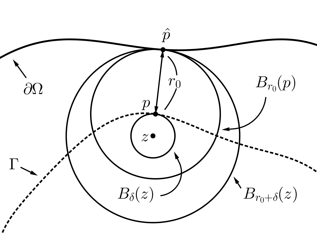
For a point $x\in\mathbb{R}^{N}$ and a number $r>0$, we set: $B_{r}(x)=\{y\in\mathbb{R}^{N}\ \mathrel{\mathop{\mathchar 58\relax}}\ |y-x|<r\}.$ Also, for a bounded $C^{2}$ domain $\Omega\subset\mathbb{R}^{N}$, $\kappa_{1}(y),\dots,\kappa_{N-1}(y)$ will always denote the principal curvatures of $\partial\Omega$ at a point $y\in\partial\Omega$ with respect to the inward normal direction to $\partial\Omega$. Then, we set

$$\Pi_{\partial\Omega}(r,y)=\prod\limits_{j=1}^{N-1}\bigl{[}1/r-\kappa_{j}(y)\bigr{]}\ \mbox{ for }\ y\in\partial\Omega\mbox{ and }r>0.$$ (3.1)

Notice that, if $B_{r}(x)\subset\Omega$ and $\overline{B_{r}(x)}\cap\partial\Omega=\{y\}$ for some $y\in\partial\Omega$, then $\kappa_{j}(y)\leq 1/r$ for all $j$’s, and hence $\Pi_{\partial\Omega}(r,y)\geq 0$.

The initial behavior of the heat content of such kind of ball is controlled by the geometry of the domain, as the following proposition explains.

Proposition D ([Sak1, Proposition 2.2, pp. 171–172]).

Let $x\in\Omega$ and assume that $B_{r}(x)\subset\Omega$ and $\overline{B_{r}(x)}\cap\partial\Omega=\{y\}$ for some $y\in\partial\Omega$. Let $u$ be the solution of either problem (1.2)–(1.4) or problem (1.5).

Then we have:

$$\lim_{t\to+0}t^{-\frac{N+1}{4}}\!\!\!\int\limits_{B_{r}(x)}\!u(z,t)\ dz=\frac{C(N,\sigma)}{\sqrt{\Pi_{\partial\Omega}(r,y)}}.$$ (3.2)

Here, $C(N,\sigma)$ is the positive constant given by

C(N,σ)={2σsN+14c(N) for problem (1.2)–(1.4,2σmσs+σmσsN+14c(N) for problem (1.5,𝐶𝑁𝜎cases2superscriptsubscript𝜎𝑠𝑁14𝑐𝑁 for problem (1.2)–(1.4missing-subexpression2subscript𝜎𝑚subscript𝜎𝑠subscript𝜎𝑚superscriptsubscript𝜎𝑠𝑁14𝑐𝑁 for problem (1.5missing-subexpressionC(N,\sigma)=\left\{\begin{array}[]{rll}2\sigma_{s}^{\frac{N+1}{4}}c(N)&\mbox{ for problem \eqref{heat equation initial-boundary}--\eqref{heat initial} },\\ \frac{2\sqrt{\sigma_{m}}}{\sqrt{\sigma_{s}}+\sqrt{\sigma_{m}}}\sigma_{s}^{\frac{N+1}{4}}c(N)&\mbox{ for problem \eqref{heat Cauchy} },\end{array}\right.

where $c(N)$ is a positive constant only depending on $N$.

When $\kappa_{j}(y)=1/r$ for some $j\in\{1,\cdots,N-1\}$, (3.2) holds by setting its right-hand side to $+\infty$

Notice that, if $\sigma_{s}=\sigma_{m}$, the constant for problem (1.5) is just half of that for problem (1.2)–(1.4).

By examining the proof of Proposition D given in [Sak1], we can also specify the initial behavior of the solution of problem (1.5).

Proposition E ([Sak1]).

As $t\to+0$, the solution $u$ of problem (1.5) converges to the number $\frac{\sqrt{\sigma_{m}}}{\sqrt{\sigma_{s}}+\sqrt{\sigma_{m}}}$, uniformly on $\partial\Omega$.

Proof.

We refer to [Sak1] for the relevant notations and formulas. In fact, the inequalities [Sak1, (22), p. 174] yield in particular that

$$(1-\varepsilon)\frac{\mu}{\theta_{-}}F_{-}(0)-2E_{1}e^{-\frac{E_{2}}{t}}\leq u(x,t)\leq(1+\varepsilon)\frac{\mu}{\theta_{+}}F_{+}(0)+2E_{1}e^{-\frac{E_{2}}{t}}\\ \mbox{ for every }(x,t)\in\partial\Omega\times(0,t_{\varepsilon}].$$

Thus,

$$(1-\varepsilon)\frac{\mu}{\theta_{-}}F_{-}(0)\leq\liminf_{t\to 0^{+}}u(x,t)\leq\limsup_{t\to 0^{+}}u(x,t)\leq(1+\varepsilon)\frac{\mu}{\theta_{+}}F_{+}(0)$$

for every $\varepsilon>0$, and hence our claim follows by observing that

$$(1-\varepsilon)\frac{\mu}{\theta_{-}}F_{-}(0)\ \mbox{ and }(1+\varepsilon)\frac{\mu}{\theta_{+}}F_{+}(0)\to\frac{\sqrt{\sigma_{m}}}{\sqrt{\sigma_{s}}+\sqrt{\sigma_{m}}}\ \mbox{ as }\varepsilon\to+0,$$

since both $F_{-}(0)$ and $F_{+}(0)$ converge to $F(0)=\frac{1}{2}$ as $\varepsilon\to+0$. ∎

We conclude this section by recalling two results from [Sak2]. The first one is a lemma that, for an elliptic equation, states the uniqueness of the reconstruction of the conductivity $\sigma$ from boundary measurements.

Lemma F ([Sak2, Lemma 3.1]).

Let $\Omega$ be a bounded $C^{2}$-regular domain in $\mathbb{R}^{N}\ (N\geq 2)$ with boundary $\partial\Omega$. Let $D_{1}$ and $D_{2}$ be two, possibly empty, bounded Lipschitz open sets, each of which may have finitely many connected components. Assume that $D_{1}\subset D_{2}\subset\overline{D_{2}}\subset\Omega$ and that both $\Omega\setminus\overline{D_{1}}$ and $\Omega\setminus\overline{D_{2}}$ are connected.

Let $\sigma_{j}\mathrel{\mathop{\mathchar 58\relax}}\Omega\to\mathbb{R}$ $(j=1,2)$ be given by

$$\sigma_{j}=\begin{cases}\sigma_{c}\quad&\mbox{in }D_{j},\\ \sigma_{s}\quad&\mbox{in }\Omega\setminus D_{j},\end{cases}$$

where $\sigma_{c},\sigma_{s}$ are positive constants with $\sigma_{c}\not=\sigma_{s}$.

For a non-zero function $g\in L^{2}(\partial\Omega)$, let $v_{j}\in H^{1}(\Omega)$ $(j=1,2)$ satisfy

$$\mbox{\rm div}(\sigma_{j}\nabla v_{j})=v_{j}-1\ \mbox{ in }\Omega\ \mbox{ and }\ \sigma_{s}{\partial_{\nu}v_{j}}=g\ \mbox{ on }\partial\Omega.$$ (3.3)

If $v_{1}=v_{2}$ on $\partial\Omega$, then $v_{1}=v_{2}$ in $\Omega$ and $D_{1}=D_{2}$.

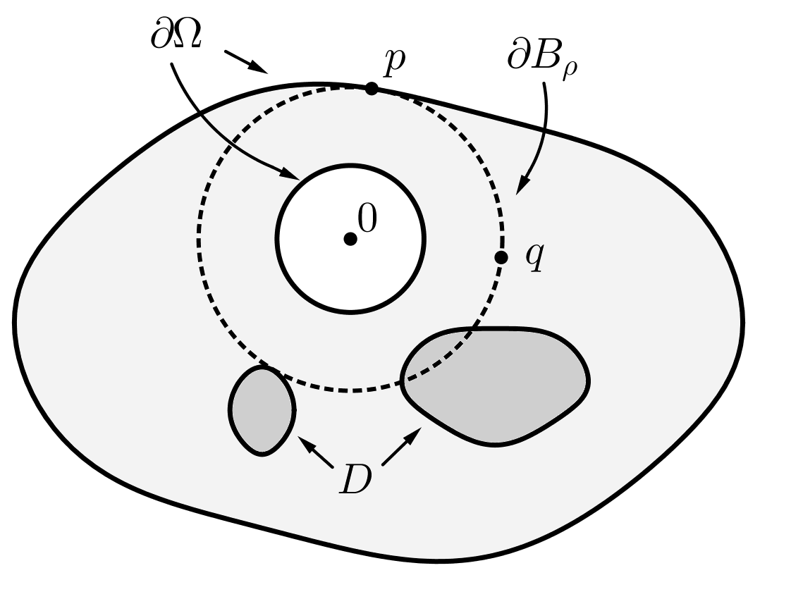
The second result from [Sak2] gives symmetry in a two-phase overdetermined problem of Serrin type in a special regime. Some preliminary notation is needed. We let $D$ be a bounded open set of class $C^{2}$, which may have finitely many connected components, compactly contained in a ball $B_{r}(x)$ and such that $B_{r}(x)\setminus\overline{D}$ is connected. Also, we denote by $\sigma\mathrel{\mathop{\mathchar 58\relax}}B_{r}(x)\to\mathbb{R}$ the conductivity distribution given by

$$\sigma=\begin{cases}\sigma_{c}\quad&\mbox{in }D,\\ \sigma_{s}\quad&\mbox{in }B_{r}(x)\setminus D,\end{cases}$$

where $\sigma_{c},\sigma_{s}$ are positive constants and $\sigma_{c}\not=\sigma_{s}$.

Theorem G ([Sak2, Theorem 5.1]).

Let $v\in H^{1}(B_{r}(x))$ be the unique solution of the following boundary value problem:

$$\mbox{\rm div}(\sigma\nabla v)=\beta v-\gamma<0\ \mbox{ in }B_{r}(x)\ \mbox{ and }\ v=c\ \mbox{ on }\partial B_{r}(x),$$ (3.4)

where $\beta\geq 0,\gamma>0$ and $c$ are real constants.

If $v$ satisfies

$$\sigma_{s}\,\partial_{\nu}v=d\ \mbox{ on }\partial B_{r}(x),$$ (3.5)

for some negative constant $d$, then $D$ must be a ball centered at $x$.

4 The constant flow property in the shell

In this section, we will carry out the proof of Theorem 1.2.

4.1 Preliminary lemmas

We start by a lemma that informs on the rough short-time asymptotic behavior of the solution of either (1.2)–(1.4) or (1.5) away from $\partial\Omega$. For $\rho>0$, we use the following notations:

$$\Omega_{\rho}=\{x\in\Omega\ \mathrel{\mathop{\mathchar 58\relax}}\mbox{ dist}(x,\partial\Omega)\geq\rho\}\ \mbox{ and }\ \Omega_{\rho}^{c}=\{x\in\mathbb{R}^{N}\setminus\Omega\ \mathrel{\mathop{\mathchar 58\relax}}\mbox{ dist}(x,\partial\Omega)\geq\rho\}.$$
Lemma 4.1.

Let $u$ be the solution of either problem (1.2)–(1.4) or (1.5).

  • (1)

    The following inequalities hold:

    $$0<u(x,t)<1\quad\mbox{ for every }(x,t)\in\Omega\times(0,+\infty)\mbox{ or }(x,t)\in\mathbb{R}^{N}\times(0,+\infty).$$
  • (2)

    For every $\rho>0$, there exist two positive constants $B$ and $b$ such that

    $$0<u(x,t)<Be^{-\frac{b}{t}}\quad\mbox{ for every }(x,t)\in\Omega_{\rho}\times(0,+\infty)$$

    and, moreover, if $u$ is the solution of (1.5), then

    $$0<1-u(x,t)<Be^{-\frac{b}{t}}\quad\mbox{ for every }(x,t)\in\Omega_{\rho}^{c}\times(0,+\infty).$$

    Here $B$ and $b$ depend only on $N,\sigma_{c},\sigma_{s},\sigma_{m}$ and $\rho$.

  • (3)

    The solution $u$ of (1.5) is such that

    $$\lim\limits_{|x|\to\infty}(1-u(x,t))=0\quad\mbox{ for every }t\in(0,+\infty).$$
Proof.

Claim (1) follows from the strong comparison principle.

To prove (2) and (3), we make use of the Gaussian bounds for the fundamental solutions of parabolic equations due to Aronson [Ar, Theorem 1, p. 891](see also [FS, p. 328]). In fact, if $g=g(x,\xi,t)$ is the fundamental solution of (1.2), there exist two positive constants $\alpha$ and $M$ depending only on $N,\sigma_{c},\sigma_{s}$ and $\sigma_{m}$ such that

$$M^{-1}t^{-\frac{N}{2}}e^{-\frac{\alpha|x-\xi|^{2}}{t}}\leq g(x,\xi,t)\leq Mt^{-\frac{N}{2}}e^{-\frac{|x-\xi|^{2}}{\alpha t}}$$ (4.1)

for all $x,\xi\in\mathbb{R}^{N}$ and $t\in(0,+\infty)$.

When $u$ is the solution of (1.5), $1-u$ can be regarded as the unique bounded solution of (1.5) with initial data ${\mathcal{X}}_{\Omega}$ in place of $\mathcal{X}_{\Omega^{c}}$. Hence we have from (4.1):

$$1-u(x,t)=\int\limits_{\mathbb{R}^{N}}g(x,\xi,t){\mathcal{X}}_{\Omega}(\xi)\ d\xi\leq Mt^{-\frac{N}{2}}\int\limits_{\Omega}e^{-\frac{|x-\xi|^{2}}{\alpha t}}d\xi.$$

Since $|x-\xi|\geq\rho$ for every $x\in\Omega_{\rho}^{c}$ and $\xi\in\Omega$, it follows that

$$t^{-\frac{N}{2}}\int\limits_{\Omega}e^{-\frac{|x-\xi|^{2}}{\alpha t}}d\xi\leq e^{-\frac{\rho^{2}}{2\alpha t}}t^{-\frac{N}{2}}\int\limits_{\Omega}e^{-\frac{|x-\xi|^{2}}{2\alpha t}}d\xi\leq(2\pi\alpha)^{\frac{N}{2}}e^{-\frac{\rho^{2}}{2\alpha t}},$$

for every $x\in\Omega_{\rho}^{c}$, being $\Omega\subset\mathbb{R}^{N}$. Thus, for any fixed $\rho>0$, the solution $u$ of (1.5) satisfies the inequality

$$1-u(x,t)\leq M(2\pi\alpha)^{\frac{N}{2}}e^{-\frac{\rho^{2}}{2\alpha t}}\ \mbox{ for every }(x,t)\in\Omega_{\rho}^{c}\times(0,+\infty),$$

which yields the second formula of (2), with $B=M\,(2\pi\alpha)^{\frac{N}{2}}$ and $b=\rho^{2}/2\alpha$, and (3), by the arbitrariness of $\rho$.

The first formula of (2) certainly holds for $t\in(1,+\infty)$, if we choose $B>0$ so large as to have that $Be^{-b}\geq 1$, since (1) holds. Therefore, it suffices to consider the case in which $t\in(0,1]$.

Let $\rho>0$, set

$$\mathcal{N}=\{x\in\mathbb{R}^{N}\mathrel{\mathop{\mathchar 58\relax}}\mbox{ dist}(x,\partial\Omega)<\rho/2\},$$

and define $v=v(x,t)$ by

$$v(x,t)=\mu\int\limits_{\mathcal{N}}g(x,\xi,t)\ d\xi\quad\mbox{ for every }(x,t)\in\mathbb{R}^{N}\times(0,+\infty).$$

Notice that $v$ is the unique bounded solution of

$$v_{t}=\mbox{ div}(\sigma\nabla v)\quad\mbox{ in }\ \mathbb{R}^{N}\times(0,+\infty)\ \mbox{ and }\ v\ =\mu{\mathcal{X}}_{\mathcal{N}}\ \mbox{ on }\mathbb{R}^{N}\times\{0\}.$$

The number $\mu>0$ can be chosen such that

$$v\geq 1\ (\geq u)\mbox{ on }\partial\Omega\times(0,1],$$

because (4.1) implies that

$$v(x,t)\geq\mu M^{-1}t^{-\frac{N}{2}}\int\limits_{\mathcal{N}}e^{-\frac{\alpha|x-\xi|^{2}}{t}}d\xi\geq\mu M^{-1}t^{-\frac{N}{2}}\int\limits_{B_{\rho/2}(0)}e^{-\frac{\alpha|\xi|^{2}}{t}}d\xi$$

for $(x,t)\in\partial\Omega\times(0,+\infty)$. Thus, the comparison principle yields that

$$u\leq v\ \mbox{ in }\Omega\times(0,1].$$ (4.2)

On the other hand, it follows from (4.1) that

$$v(x,t)\leq\mu Mt^{-\frac{N}{2}}\int\limits_{\mathcal{N}}e^{-\frac{|x-\xi|^{2}}{\alpha t}}d\xi\quad\mbox{ for }(x,t)\in\mathbb{R}^{N}\times(0,+\infty)$$

and hence, since $|x-\xi|\geq\rho/2$ for every $x\in\Omega_{\rho}$ and $\xi\in\mathcal{N}$, we obtain that

$$v(x,t)\leq\mu Mt^{-\frac{N}{2}}e^{-\frac{\rho^{2}}{8\alpha t}}\int\limits_{\mathbb{R}^{N}}e^{-\frac{|x-\xi|^{2}}{2\alpha t}}d\xi=\mu M(2\pi\alpha)^{\frac{N}{2}}e^{-\frac{\rho^{2}}{8\alpha t}}$$

for every $(x,t)\in\Omega_{\rho}\times(0,+\infty)$.

This inequality and (4.2) then yield the first formula of (2). ∎

Next lemma informs us that, as in the case of stationary level surfaces, surfaces having the constant flow property satisfy a certain balance law.

Lemma 4.2 (A balance law).

Let $\Gamma$ be a connected component of class $C^{2}$ of $\partial G$ satisfying (1.7). Set $r_{0}=\mbox{\rm dist}(\Gamma,\partial\Omega)(>0).$

Let $u$ be the solution of either problem (1.2)–(1.4) or (1.5). Then, (1.10) holds if and only if there exists a function $c\mathrel{\mathop{\mathchar 58\relax}}(0,r_{0})\times(0,+\infty)\to\mathbb{R}$ such that

$$\int_{B_{r}(x)}u(y,t)\,(y-x)\cdot\nu(x)\,dy=c(r,t)\ \mbox{ for every }\ (x,r,t)\in\Gamma\times(0,r_{0})\times(0,+\infty),$$ (4.3)

where $\nu=\nu(x)$ denotes the outward unit normal vector to $\Gamma$ at $x\in\Gamma$.

Proof.

Since $\Gamma$ is compact, let $p\in\Gamma$ be a point such that $\mathop{\mathrm{dist}}(p,\partial\Omega)=r_{0}$. If (1.10) holds, we have that

$$d(t)=\sigma_{s}\nabla u(p,t)\cdot\nu(p)=\sigma_{s}\nabla u(q,t)\cdot\nu(q)\ \mbox{ for every }(q,t)\in\Gamma\times(0,+\infty).$$ (4.4)

Next, fix a $q\in\Gamma$ and let $A$ be an orthogonal matrix satisfying

$$A\nu(p)=\nu(q).$$ (4.5)

From (4.4) and (4.5) we obtain that the function $v=v(x,t)$, defined by

$$v(x,t)=u(x+p,t)-u(Ax+q,t)\ \mbox{ for }(x,t)\in B_{r_{0}}(0)\times(0,+\infty),$$

is such that

$$\nabla v(0,t)\cdot\nu(p)=\nabla u(p,t)\cdot\nu(p)-[A^{T}\nabla u(q,t)]\cdot\nu(p)=\\ \nabla u(p,t)\cdot\nu(p)-\nabla u(q,t)\cdot[A\,\nu(p)]=\nabla u(p,t)\cdot\nu(p)-\nabla u(q,t)\cdot\nu(q)=0,$$

for every $t>0$. Here, the superscript $T$ stands for transpose.

Now, since assumption (1.6) guarantees that $B_{r_{0}}(p)$ and $B_{r_{0}}(q)\subset\Omega\setminus\overline{D}$, and $\sigma=\sigma_{s}$ in $\Omega\setminus\overline{D}$, we have that $v$ satisfies the heat equation with constant conductivity $\sigma_{s}$:

$$v_{t}=\sigma_{s}\Delta v\ \mbox{ in }\ B_{r_{0}}(0)\times(0,+\infty).$$

Thus, also the function $\nabla v(x,t)\cdot\nu(p)$ satisfies the same equation and we have seen that $\nabla v(0,t)\cdot\nu(p)=0$ for every $t>0$. Hence, we can use a balance law (see [MS2, Theorem 2.1, pp. 934–935] or [MS1, Theorem 4, p. 704]) to obtain that

$$\int\limits_{\partial B_{r}(0)}\!\!\nabla v(y,t)\cdot\nu(p)\,dS_{y}=0\ \mbox{ for every }\ (r,t)\in(0,r_{0})\times(0,+\infty)$$

or, by integrating this in $r$, that

$$\int\limits_{B_{r}(0)}\!\!\nabla v(y,t)\cdot\nu(p)\,dy=0\ \mbox{ for every }\ (r,t)\in(0,r_{0})\times(0,+\infty).$$

By the divergence theorem and again integrating in $r$, we then get

$$\int\limits_{B_{r}(0)}\!\!v(y,t)\,y\cdot\nu(p)\,dy=0\ \mbox{ for every }\ (r,t)\in(0,r_{0})\times(0,+\infty),$$

that is

$\displaystyle\int\limits_{B_{r}(p)}\!\!u(y,t)(y-p)\cdot\nu(p)\,dy=\int\limits_{B_{r}(q)}\!\!u(y,t)(y-q)\cdot\nu(q)\,dy$ (4.6)
 $\displaystyle\qquad\qquad\mbox{ for every }\ (q,r,t)\in\Gamma\times(0,r_{0})\times(0,+\infty).$

Therefore, (4.3) ensues.

It is not difficult to show that (4.3) implies (1.10). ∎

The following lemma is decisive to prove Theorem 1.2. Among other things, it states that, as in the case of stationary isothermic surfaces, also surfaces having the constant flow property are parallel to a connected component of $\partial\Omega$.

Lemma 4.3.

Let $u$ be the solution of either problem (1.2)–(1.4) or (1.5), and let $\Gamma$ be a connected component of class $C^{2}$ of $\partial G$ satisfying (1.7). Under the assumption (1.10) of Theorem 1.2, the following assertions hold:

  1. (1)

    there exists a number $r_{0}>0$ such that

    $$\mbox{\rm dist}(x,\partial\Omega)=r_{0}\ \mbox{ for every }x\in\Gamma;$$
  2. (2)

    $\Gamma$ is a real analytic hypersurface;

  3. (3)

    there exists a connected component $\gamma$ of $\partial\Omega$, that is also a real analytic hypersurface, such that the mapping $\gamma\ni y\mapsto x(y)\equiv y-r_{0}\,\nu(y)\in\Gamma$ is a diffeomorphism; in particular $\gamma$ and $\Gamma$ are parallel hypersurfaces at distance $r_{0}$;

  4. (4)

    it holds that

    $$\kappa_{j}(y)<\frac{1}{r_{0}}\ \mbox{ for every }y\in\gamma\mbox{ and }\ j=1,\dots,N-1;$$
  5. (5)

    there exists a number $c_{0}>0$ such that $\Pi_{\partial\Omega}(r_{0},y)=c_{0}$ for every $y\in\gamma$, where $\Pi_{\partial\Omega}$ is given in (3.1).

Proof.

We just have to prove assertion (1): the remaining ones then will easily follow.

Let $r_{0}>0$ be the minimum of $\mathop{\mathrm{dist}}(x,\partial\Omega)$ for $x\in\Gamma$ and suppose it is achieved at $p$; assume that there exists a point $q_{*}\in\Gamma$ such that

$$r_{0}<\mathop{\mathrm{dist}}(q_{*},\partial\Omega).$$

Since $\overline{B_{r_{0}}(q_{*})}\subset\Omega$, with the aid of Lemma 4.1 we have:

$$\lim_{t\to+0}t^{-\frac{N+1}{4}}\!\!\!\int\limits_{B_{r_{0}}(q_{*})}\!\!u(x,t)\,(x-q_{*})\cdot\nu(q_{*})\,dx=0.$$ (4.7)

In view of (1.7), since $r_{0}=\mbox{ dist}(p,\partial\Omega)=\mbox{ dist}(\partial G,\partial\Omega)=\mbox{ dist}(\overline{G},\partial\Omega)$ and $\Gamma$ is of class $C^{2}$, we can find a ball $B_{\delta}(z)\subset G$ satisfying

$$\overline{B_{\delta}(z)}\cap\partial G=\{p\}\ \mbox{ and }\ B_{\delta+r_{0}}(z)\subset\Omega.$$

Also, by setting $\hat{p}=p+r_{0}\nu(p)\ (\in\partial\Omega)$ we have:

$$\overline{B_{r_{0}}(p)}\cap\partial\Omega=\{\hat{p}\}\ \mbox{ and }\ \kappa_{j}(\hat{p})\leq\frac{1}{r_{0}+\delta}<\frac{1}{r_{0}}\ \mbox{ for }j=1,\dots,N-1.$$ (4.8)
Refer to caption
Figure 2: The three-balls construction.

Thus, Proposition D gives that

$$\lim_{t\to+0}t^{-\frac{N+1}{4}}\!\!\!\int\limits_{B_{r_{0}}(p)}\!\!u(x,t)\ dx=\frac{C(N,\sigma)}{\sqrt{\Pi_{\partial\Omega}(r_{0},\hat{p})}}.$$ (4.9)

On the other hand, by Lemma 4.1 and the fact that $\overline{B_{r_{0}}(p)}\cap\partial\Omega=\{\hat{p}\}$, we have

$$\lim_{t\to+0}t^{-\frac{N+1}{4}}\!\!\!\!\!\!\!\!\!\!\int\limits_{B_{r_{0}}(p)\setminus B_{\varepsilon}(\hat{p})}\!\!\!\!\!\!u(x,t)\ dx=0\ \mbox{ for every }\varepsilon>0.$$ (4.10)

Therefore, combining the last two formulas yields that

$$\lim_{t\to+0}t^{-\frac{N+1}{4}}\!\!\!\int\limits_{B_{r_{0}}(p)}\!\!u(x,t)(x-p)\cdot\nu(p)\,dx=r_{0}\,\frac{C(N,\sigma)}{\sqrt{\Pi_{\partial\Omega}(r_{0},\hat{p})}}.$$ (4.11)

In fact, for every $\varepsilon>0$, we have

$\displaystyle\left|t^{-\frac{N+1}{4}}\!\!\!\!\!\!\!\!\!\int\limits_{B_{r_{0}}(p)\cap B_{\varepsilon}(\hat{p})}\!\!\!\!\!\!\!\!u(x,t)(x-\hat{p})\cdot\nu(p)\,dx\right|\leq\varepsilon t^{-\frac{N+1}{4}}\!\!\!\int\limits_{B_{r_{0}}(p)}\!\!u(x,t)\,dx,$ (4.12)
$\displaystyle\left|t^{-\frac{N+1}{4}}\!\!\!\!\!\!\!\!\!\int\limits_{B_{r_{0}}(p)\setminus B_{\varepsilon}(\hat{p})}\!\!\!\!\!\!\!\!u(x,t)(x-\hat{p})\cdot\nu(p)\,dx\right|\leq 2r_{0}t^{-\frac{N+1}{4}}\!\!\!\!\!\!\!\!\!\int\limits_{B_{r_{0}}(p)\setminus B_{\varepsilon}(\hat{p})}\!\!\!\!\!\!\!\!u(x,t)\,dx.$ (4.13)

Moreover, since $(\hat{p}-p)\cdot\nu(p)=r_{0}$, we have that

$$t^{-\frac{N+1}{4}}\!\!\!\!\!\!\int\limits_{B_{r_{0}}(p)}\!\!u(x,t)(x-p)\cdot\nu(p)\,dx=r_{0}\,t^{-\frac{N+1}{4}}\!\!\!\!\!\!\int\limits_{B_{r_{0}}(p)}\!\!u(x,t)\,dx+\\ t^{-\frac{N+1}{4}}\!\!\!\!\!\!\!\!\!\!\!\!\int\limits_{B_{r_{0}}(p)\setminus B_{\varepsilon}(\hat{p})}\!\!\!\!\!\!\!\!u(x,t)(x-\hat{p})\cdot\nu(p)\,dx+t^{-\frac{N+1}{4}}\!\!\!\!\!\!\!\!\!\!\!\!\int\limits_{B_{r_{0}}(p)\cap B_{\varepsilon}(\hat{p})}\!\!\!\!\!\!\!\!u(x,t)(x-\hat{p})\cdot\nu(p)\,dx,$$

for every $t>0$. Therefore, combining (4.9), (4.10), (4.12) and (4.13) yields that

$\displaystyle(r_{0}-\varepsilon)\,\frac{C(N,\sigma)}{\sqrt{\Pi_{\partial\Omega}(r_{0},\hat{p})}}\leq\liminf_{t\to+0}\ t^{-\frac{N+1}{4}}\!\!\!\int\limits_{B_{r_{0}}(p)}\!\!u(x,t)(x-p)\cdot\nu(p)\,dx$
$\displaystyle\leq\limsup_{t\to+0}\ t^{-\frac{N+1}{4}}\!\!\!\int\limits_{B_{r_{0}}(p)}\!\!u(x,t)(x-p)\cdot\nu(p)\,dx\leq(r_{0}+\varepsilon)\,\frac{C(N,\sigma)}{\sqrt{\Pi_{\partial\Omega}(r_{0},\hat{p})}}$

for every $\varepsilon>0$, which gives (4.11).

It is clear that (4.11) contradicts (4.7) and the balance law (4.3), and hence assertion (1) holds true.

Now, once we have (1), we can apply the same argument as above to any other point in $\Gamma$. Thus, we know from (4.3), (4.8) and (4.11) that there exists a connected component $\gamma$ of $\partial\Omega$ satisfying (3), (4) and (5). The analyticity of $\gamma$ follows from (4) and (5). Indeed, by using local coordinates, the condition (5) with (4) can be converted into a second order analytic nonlinear elliptic equation of Monge-Ampère type, where (4) guarantees the ellipticity as is noted in [MS2, p. 945]. Hence (2) is implied by (3) together with (4). ∎

4.2 Proof of Theorem 1.2 for problem (1.2)–(1.4)

Let $u$ be the solution of problem (1.2)–(1.4). By virtue of (1) of Lemma 4.1, we can define the function $v\mathrel{\mathop{\mathchar 58\relax}}\overline{\Omega}\to\mathbb{R}$ by the Laplace transform of $1-u(x,\cdot)$ computed at the complex parameter $1+0\sqrt{-1}$

$$v(x)=\int_{0}^{\infty}e^{-t}[1-u(x,t)]\,dt\quad\mbox{ for }x\in\overline{\Omega},$$ (4.14)

and set $U=v$ on $\overline{\Omega}\setminus D$ and $V=v$ on $\overline{D}$. Then, it is easy to show that

$\displaystyle 0<U<1\mbox{ in }\Omega\setminus\overline{D},\quad 0<V<1\mbox{ in }D,$ (4.15)
$\displaystyle\sigma_{s}\,\Delta U=U-1\mbox{ in }\Omega\setminus\overline{D},\quad\sigma_{c}\,\Delta V=V-1\mbox{ in }D,$ (4.16)
$\displaystyle U=V\ \mbox{ and }\ \sigma_{s}\,\partial_{\nu}U=\sigma_{c}\,\partial_{\nu}V\ \mbox{ on }\partial D,$ (4.17)
$\displaystyle U=0\ \mbox{ on }\partial\Omega.$ (4.18)

Here, $\nu$ denotes the outward unit normal vector to $\partial D$ at points of $\partial D$. The two equations in (4.17) follow from the transmission condition satisfied by $u$ on $\partial D\times(0,+\infty)$ and involve the continuous extensions of the relevant functions up to $\partial D$.

Next, let $\gamma$ be the connected component of $\partial\Omega$ whose existence is guaranteed by Lemma 4.3. Claims (5) and (4) of Lemma 4.3 also tell us that $\gamma$ is an elliptic Weingarten-type surface, that is its principal curvatures satisfy a symmetric constraint which can be recast as an elliptic partial differential equation, considered by Aleksandrov’s sphere theorem [Al, p. 412], and hence $\gamma$ is a sphere. Consequently, $\Gamma$ is a sphere concentric with $\gamma$; we can always assume that the origin is their common center.

By combining the initial and boundary conditions of problem (1.2)–(1.4) and the assumption (1.10) with the real analyticity in $x$ of $u$ over $\Omega\setminus\overline{D}$, we see that $u$ is radially symmetric in $x$ on $\overline{\Omega}\setminus D$ for every $t>0$. Here, we used the fact that $\Omega\setminus\overline{D}$ is connected. Moreover, in view of (1.3), we can distinguish two cases:

$$\mbox{\rm(I) }\Omega\mbox{ is a ball;}\qquad\mbox{\rm(II) }\Omega\mbox{ is a spherical shell.}$$

We first show that case (II) never occurs. Suppose that $\Omega=B_{\rho_{+}}\setminus\overline{B_{\rho_{-}}}$ where $B_{\rho_{+}}$ and $B_{\rho_{-}}$ are two balls centered at the origin with $\rho_{+}>\rho_{-}>0$. By the radial symmetry of $u$ on $\Omega\setminus\overline{D}$ for every $t>0$, being $\Omega\setminus\overline{D}$ connected, there exists a function $\widetilde{U}\mathrel{\mathop{\mathchar 58\relax}}[\rho_{-},\rho_{+}]\to\mathbb{R}$ such that $U(x)=\widetilde{U}(|x|)$ for $x\in\overline{\Omega}\setminus D$. Moreover, by (4.16), $\widetilde{U}$ is extended as a solution of

$$\sigma_{s}\left(\partial_{rr}\widetilde{U}+\frac{N-1}{r}\partial_{r}\widetilde{U}\right)=\widetilde{U}-1\ \mbox{ for all }r>0,$$

where $\partial_{r}$ and $\partial_{rr}$ stand for first and second derivatives with respect to the variable $r=|x|$. That means that $U$ is extended as a radially symmetric solution of $\sigma_{s}\Delta U=U-1$ in $\mathbb{R}^{N}\setminus\{0\}$. By applying Hopf’s boundary point lemma (see [GT, Lemma 3.4, p. 34]) to $U$, we obtain from (4.15), (4.16) and (4.18) that

$\displaystyle\sigma_{s}\Delta U=U-1<0\ \mbox{ in }\Omega,$ (4.19)
$\displaystyle\partial_{\nu}U=-\partial_{r}\widetilde{U}(\rho_{-})<0\ \mbox{ on }\partial B_{\rho_{-}}\ \mbox{ and }\ \partial_{\nu}U=\partial_{r}\widetilde{U}(\rho_{+})<0\ \mbox{ on }\partial B_{\rho_{+}}.$ (4.20)

Now, we use Lemma F. We set $D_{1}=\varnothing$, $D_{2}=D$, and consider two functions $v_{j}\in H^{1}(\Omega)\ (j=1,2)$ defined by

$$v_{1}=U\ \mbox{ and }v_{2}=\left\{\begin{array}[]{rll}U&\mbox{ in }\ \Omega\setminus D,\\ V&\mbox{ in }\ D.\end{array}\right.$$

In view of (4.16), (4.17), (4.18), (4.19) and (4.20), Lemma F gives that $v_{1}=v_{2}$ in $\Omega$ and $\varnothing=D$, which is a contradiction. Thus, case (II) never occurs.

It remains to consider case (I), that is we assume that $\Omega$ is a ball $B_{R}$ centered at the origin for some radius $R>0$.

Since $u$ is radially symmetric on $\overline{\Omega}\setminus D$ for every $t>0$ and $\Omega\setminus\overline{D}$ is connected, by applying Hopf’s boundary point lemma to the radially symmetric function $U$, we obtain from (4.15), (4.16) and (4.18) that

$$\sigma_{s}\,\partial_{\nu}U=\sigma_{s}\,\partial_{r}\widetilde{U}(R)<0\ \mbox{ on }\partial B_{R}.$$ (4.21)

Thus, in view of (4.15), (4.16) and (4.18), we see that the function $v$ defined in (4.14) satisfies

$$\mbox{\rm div}(\sigma\nabla v)=v-1<0\ \mbox{ in }B_{R}\ \mbox{ and }\ v=0\ \mbox{ on }\partial B_{R}.$$

Therefore, with the aid of (4.21), we can apply Theorem G to $v$ to see that $D$ must be a ball centered at the origin.

4.3 Proof of Theorem 1.2 for problem (1.5)

Let $u$ be the solution of problem (1.5). We proceed similarly to Subsection 4.2. This time, by virtue of (1) of Lemma 4.1, we define a function $v\mathrel{\mathop{\mathchar 58\relax}}\mathbb{R}^{N}\to\mathbb{R}$ by

$$v(x)=\int_{0}^{\infty}e^{-t}[1-u(x,t)]\,dt\quad\mbox{ for every }\ x\in\mathbb{R}^{N}$$ (4.22)

and, in addition to the already defined functions $U$ and $V$, we set $W=v$ on $\mathbb{R}^{N}\setminus\overline{\Omega}$.

While $U$ and $V$ satisfy (4.15)-(4.17), $W$ satisfies

$\displaystyle 0<W<1\ \mbox{ in }\ \mathbb{R}^{N}\setminus\overline{\Omega},$ (4.23)
$\displaystyle\sigma_{m}\,\Delta W=W\ \mbox{ in }\ \mathbb{R}^{N}\setminus\overline{\Omega},$ (4.24)
$\displaystyle W=U\ \mbox{ and }\ \sigma_{m}\,\partial_{\nu}W=\sigma_{s}\,\partial_{\nu}U\ \mbox{ on }\partial\Omega,$ (4.25)
$\displaystyle\lim_{|x|\to\infty}W(x)=0.$ (4.26)

Similarly to Subsection 4.2, $\nu$ denotes the outward unit normal vector to $\partial D$ or to $\partial\Omega$, and both (4.17) and (4.25) are consequences of the transmission conditions satisfied by $u$ on $\partial D\times(0,+\infty)$ and on $\partial\Omega\times(0,+\infty)$, respectively. Also, to obtain (4.26), we used Lemma 4.1 together with Lebesgue’s dominated convergence theorem.

Again, by Aleksandrov’s sphere theorem [Al, p. 412], Lemma 4.3 yields that $\gamma$ and $\Gamma$ are concentric spheres, with a common center that we can place at the origin. Being $\Omega\setminus\overline{D}$ connected, the radial symmetry of $u$ in $x$ on $\overline{\Omega}\setminus D$ for every $t>0$ is obtained similarly, by combining the initial condition in (1.5) and the assumption (1.10) with the real analyticity in $x$ of $u$ over $\Omega\setminus\overline{D}$.

Moreover, in view of the initial condition of problem (1.5) and Proposition E, we can prove that $\Omega$ is radially symmetric and hence $u$ is radially symmetric in $x$ on $\mathbb{R}^{N}\setminus D$ for every $t>0$. Indeed, if there exists another connected component $\hat{\gamma}$ of $\partial\Omega$, which is not a sphere centered at the origin, we can find a number $\rho>0$ and two points $p\in\partial\Omega,q\in\Omega\setminus\overline{D}$ such that

$$\partial B_{\rho}\subset\overline{\Omega},\ p\in\hat{\gamma}\cap\partial B_{\rho},\ \mbox{ and }q\in(\Omega\setminus\overline{D})\cap\partial B_{\rho},$$

being $B_{\rho}$ the ball centered at the origin with radius $\rho$.

Refer to caption
Figure 3: The ball construction for the Cauchy problem.

Then, since $u$ is radially symmetric on $\overline{\Omega}\setminus D$ for every $t>0$, we have:

$$u(p,t)=u(q,t)\ \mbox{ for every }t>0.$$ (4.27)

On the other hand, by Proposition E $\lim\limits_{t\to+0}u(p,t)=\frac{\sqrt{\sigma_{m}}}{\sqrt{\sigma_{s}}+\sqrt{\sigma_{m}}}$ and by (2) of Lemma 4.1 $\lim\limits_{t\to+0}u(q,t)=0$. These contradict (4.27). Once we know that $\Omega$ is radially symmetric, the radial symmetry of $u$ on $\mathbb{R}^{N}\setminus D$ for every $t>0$ follows from the initial condition in (1.5).

Thus, as in the previous case, we can distinguish two cases:

$$\mbox{\rm(I) }\Omega\mbox{ is a ball;}\qquad\mbox{\rm(II) }\Omega\mbox{ is a spherical shell.}$$

We first show that case (II) never occurs. With the same notations as in Subsection 4.2, we set $\Omega=B_{\rho_{+}}\setminus\overline{B_{\rho_{-}}}$. Since $u$ is radially symmetric in $x$ on $\mathbb{R}^{N}\setminus D$ for every $t>0$, so is $W$ on $\mathbb{R}^{N}\setminus D$. Observe from (4.23) and (4.24) that

$$\Delta W>0\ \mbox{ in }B_{\rho_{-}}\mbox{ and }\mathbb{R}^{N}\setminus\overline{B_{\rho_{+}}}.$$

Therefore, in view of (4.26), the strong maximum principle tells us that the positive maximum value of $W$ on $\overline{B_{\rho_{-}}}$ or on $\mathbb{R}^{N}\setminus B_{\rho_{+}}$ is achieved only on $\partial B_{\rho_{-}}$ or $\partial B_{\rho_{+}}$, respectively. Hence, since $W$ is radially symmetric, Hopf’s boundary point lemma yields that

$$\partial_{\nu}W<0\mbox{ on }\partial B_{\rho_{-}}\mbox{ and }\partial B_{\rho_{+}}.$$ (4.28)

As in Subsection 4.2, $U$ is extended as a radially symmetric solution of $\sigma_{s}\,\Delta U=U-1$ in $\mathbb{R}^{N}\setminus\{0\}$. Then, it follows from (4.28), (4.15) and (4.25) that both (4.19) and (4.20) also hold true. Therefore, with the aid of Lemma F, by the same argument of the proof in Subsection 4.2, we obtain a contradiction, and hence case (II) never occurs.

It remains to consider case (I). As in Subsection 4.2, we set $\Omega=B_{R}.$ Since $u$ is radially symmetric in $x$ on $\mathbb{R}^{N}\setminus\overline{D}$ for every $t>0$, $W$ is also radially symmetric on $\mathbb{R}^{N}\setminus\overline{D}$. Observe from (4.23) and (4.24) that

$$\Delta W>0\ \mbox{ in }\mathbb{R}^{N}\setminus\overline{B_{R}}.$$

Therefore, in view of (4.26), the strong maximum principle informs us that the positive maximum value of $W$ on $\mathbb{R}^{N}\setminus B_{R}$ is achieved only on $\partial B_{R}$. Hence, since $W$ is radially symmetric, Hopf’s boundary point lemma yields that

$$\partial_{\nu}W<0\ \mbox{ on }\ \partial B_{R}.$$ (4.29)

Combining (4.29) with (4.25) implies that both $U$ and $\partial_{\nu}U$ are constant on $\partial B_{R}$. Therefore, with the aid of Theorem G and by the same argument of the proof in Subsection 4.2, we conclude that $D$ must be a ball centered at the origin.

4.4 Proof of Theorem 1.3

In view of the statements of Theorems 1.3, A and B, it suffices to show that Theorem B can be improved as in Theorem A. Namely, in proposition (b) of Theorem B we may show that the assumption that $\sigma_{s}=\sigma_{m}$ is not necessary.

Let in fact $u$ be the solution of problem (1.5). Aleksandrov’s sphere theorem [Al, p. 412] and [Sak1, Lemma 2.4, p. 176] yield that $\gamma$ and $\Gamma$ are concentric spheres. Then, with the aid of the initial condition of problem (1.5) and Proposition E, we can observe that the rest of the proof runs as in the proof given in Subsection 4.3.

5 The constant flow property at the boundary

In this section, we will give the proofs of Theorems 1.4 and 1.5 .

Let $u$ be the solution of problem (1.2)–(1.4), and let $\Gamma$ be a connected component of $\partial\Omega$. We introduce the distance function $\delta=\delta(x)$ of $x\in\mathbb{R}^{N}$ to $\Gamma$ by

$$\delta(x)=\mbox{ dist}(x,\Gamma)\ \mbox{ for }\ x\in\mathbb{R}^{N}.$$ (5.1)

Since $\Gamma$ is of class $C^{6}$ and compact, by choosing a number $\delta_{0}>0$ sufficiently small and setting

$$\mathcal{N}_{0}=\{x\in\Omega\ \mathrel{\mathop{\mathchar 58\relax}}\ 0<\delta(x)<\delta_{0}\},$$ (5.2)

we see that

$\displaystyle\overline{\mathcal{N}_{0}}\cap\overline{D}=\varnothing,\ \delta\in C^{6}(\overline{\mathcal{N}_{0}}),$ (5.3)
$\displaystyle\mbox{ for every }x\in\overline{\mathcal{N}_{0}}\mbox{ there exists a unique }y=y(x)\in\Gamma\mbox{ with }\delta(x)=|x-y|,$ (5.4)
$\displaystyle y(x)=x-\delta(x)\nabla\delta(x)\ \mbox{ for all }x\in\overline{\mathcal{N}_{0}},$ (5.5)
$\displaystyle\max_{1\leq j\leq N-1}\kappa_{j}(y)<\frac{1}{2\delta_{0}}\ \mbox{ for every }y\in\Gamma.$ (5.6)

The principal curvatures $\kappa_{j}$ of $\Gamma$ are taken at $y$ with respect to the inward unit normal vector $-\nu(y)=\nabla\delta(y)$ to $\partial\Omega$.

5.1 Introducing a Laplace transform

Let us define the function $w=w(x,\lambda)$ by the Laplace-Stieltjes transform of $u(x,\cdot)$ or the Laplace transform of $u_{t}(x,\cdot)$ restricted on the semiaxis of real positive numbers

$$w(x,\lambda)=\lambda\int_{0}^{\infty}e^{-\lambda t}u(x,t)\ dt\ \mbox{ for }(x,\lambda)\in\Omega\times(0,+\infty).$$

Notice that letting $\lambda=1$ gives

$$w(x,1)=1-v(x)\ \mbox{ for every }x\in\Omega,\mbox{ and }w(x,1)=1-U(x)\mbox{ for }x\in\Omega\setminus D,$$ (5.7)

where $v$ is the function defined by (4.14) and $U={\left.\kern-1.2ptv\vphantom{|}\right|_{\overline{\Omega}\setminus D}}$.

Next, we observe that for every $\lambda>0$

$\displaystyle\mbox{ div}(\sigma\nabla w)-\lambda w=0\ \mbox{ and }\ 0<w<1$ $\displaystyle\mbox{ in }\Omega,$ (5.8)
$\displaystyle w=1$ $\displaystyle\mbox{ on }\partial\Omega.$ (5.9)

Hence, by the assumption (1.10), there exists a function $d_{0}\mathrel{\mathop{\mathchar 58\relax}}(0,\infty)\to\mathbb{R}$ satisfying

$$\sigma_{s}\,\partial_{\nu}w(x,\lambda)=d_{0}(\lambda)\ \mbox{ for every }(x,\lambda)\in\Gamma\times(0,+\infty).$$ (5.10)

Moreover, it follows from the first formula of (2) of Lemma 4.1 that there exist two positive constants $\widetilde{B}$ and $\widetilde{b}$ satisfying

$$0<w(x,\lambda)\leq\widetilde{B}e^{-\widetilde{b}\sqrt{\lambda}}\ \mbox{ for every }(x,\lambda)\in\left(\partial\mathcal{N}_{0}\cap\Omega\right)\times(0,+\infty).$$ (5.11)

5.2 Two auxiliary functions

Since $w$ satisfies (5.9) and $\Delta w-\frac{\lambda}{\sigma_{s}}w=0$ in $\mathcal{N}_{0}$, in view of the formal WKB approximation of $w$ for sufficiently large $\tau=\frac{\lambda}{\sigma_{s}}$

$$w(x,\lambda)\sim e^{-\sqrt{\tau}\delta(x)}\sum_{j=0}^{\infty}A_{j}(x)\tau^{-\frac{j}{2}}\ \mbox{ with some coefficients }\{A_{j}(x)\},$$

we introduce two functions $f_{\pm}=f_{\pm}(x,\lambda)$ defined for $(x,\lambda)\in\overline{\mathcal{N}_{0}}\times(0,+\infty)$ by

$$f_{\pm}(x,\lambda)=e^{-\frac{\sqrt{\lambda}}{\sqrt{\sigma_{s}}}\delta(x)}\left[A_{0}(x)+\frac{\sqrt{\sigma_{s}}}{\sqrt{\lambda}}A_{\pm}(x)\right],$$

where

$\displaystyle A_{0}(x)=\left\{\prod\limits_{j=1}^{N-1}\Bigl{[}1-\kappa_{j}(y(x))\delta(x)\Bigr{]}\right\}^{-\frac{1}{2}},$
$\displaystyle A_{\pm}(x)=\int_{0}^{\delta(x)}\left[\frac{1}{2}\,\Delta A_{0}(x(\tau))\pm 1\right]\exp\left(-\frac{1}{2}\,\int_{\tau}^{\delta(x)}\Delta\delta(x(\tau^{\prime}))d\tau^{\prime}\right)d\tau,$

with $x(\tau)=y(x)-\tau\,\nu(y(x))$ for $0<\tau<\delta(x)$. It is shown in [GT, Lemmas 14.16 and 14.17, p. 355] that

$$|\nabla\delta(x)|=1\ \mbox{ and }\ \Delta\delta(x)=-\sum_{j=1}^{N-1}\frac{\kappa_{j}(y(x))}{1-\kappa_{j}(y(x))\delta(x)}.$$

With these in hand, by straightforward computations we obtain that

$$\nabla\delta\cdot\nabla A_{0}=-\frac{1}{2}(\Delta\delta)A_{0},\quad\nabla\delta\cdot\nabla A_{\pm}=-\frac{1}{2}(\Delta\delta)A_{\pm}+\frac{1}{2}\Delta A_{0}\pm 1\ \mbox{ in }\ \overline{\mathcal{N}_{0}},$$ (5.12)
$$\sigma_{s}\Delta f_{\pm}-\lambda f_{\pm}=\sigma_{s}e^{-\frac{\sqrt{\lambda}}{\sqrt{\sigma_{s}}}\delta(x)}\left(\mp 2+\frac{\sqrt{\sigma_{s}}}{\sqrt{\lambda}}\Delta A_{\pm}\right)\ \mbox{ in }\ \overline{\mathcal{N}_{0}},$$ (5.13)

and

$$A_{0}=1,\ A_{\pm}=0,\quad f_{\pm}=1\ \mbox{ on }\ \Gamma,$$ (5.14)

for every $\lambda>0$.

Since $\Gamma$ is of class $C^{6}$ and compact, we observe from (5.3)–(5.6) that

$$|\Delta A_{\pm}|\leq c_{0}\ \mbox{ in }\overline{\mathcal{N}_{0}},$$

for some positive constant $c_{0}$. Therefore, it follows from (5.13), (5.11) and the definition of $f_{\pm}$ that there exist two positive constants $\lambda_{0}$ and $\eta$ such that

$\displaystyle\sigma_{s}\Delta f_{+}-\lambda f_{+}<0<\sigma_{s}\Delta f_{-}-\lambda f_{-}\ \mbox{ in }\ \overline{\mathcal{N}_{0}},$ (5.15)
$\displaystyle\max\{|f_{+}|,|f_{-}|,w\}\leq e^{-\eta\sqrt{\lambda}}\ \mbox{ on }\ \partial\mathcal{N}_{0}\cap\Omega,$ (5.16)

for every $\lambda\geq\lambda_{0}$.

5.3 Construction of barriers for $w(x,\lambda)$

Let $\psi=\psi(x)$ be the unique solution of the Dirichlet problem:

$$\Delta\psi=0\ \mbox{ in }\ \mathcal{N}_{0},\quad\psi=0\ \mbox{ on }\ \Gamma,\quad\psi(x)=2\ \mbox{ on }\ \partial\mathcal{N}_{0}\cap\Omega.$$

For every $(x,\lambda)\in\overline{\mathcal{N}_{0}}\times(0,+\infty)$, we define the two functions $w_{\pm}=w_{\pm}(x,\lambda)$ by

$$w_{\pm}(x,\lambda)=f_{\pm}(x,\lambda)\pm\psi(x)e^{-\eta\sqrt{\lambda}}.$$

Then, in view of (5.8), (5.9), (5.14), (5.15) and (5.16), we notice that

$\displaystyle\sigma_{s}\Delta w_{+}-\lambda w_{+}<0=\sigma_{s}\Delta w-\lambda w<\sigma_{s}\Delta w_{-}-\lambda w_{-}$ $\displaystyle\mbox{ in }\mathcal{N}_{0},$
$\displaystyle w_{+}=w=w_{-}=1$ $\displaystyle\mbox{ on }\Gamma,$
$\displaystyle w_{-}<w<w_{+}$ $\displaystyle\mbox{ on }\partial\mathcal{N}_{0}\cap\Omega,$

for every $\lambda\geq\lambda_{0}$, and hence we get that

$$w_{-}<w<w_{+}\ \mbox{ in }\ \mathcal{N}_{0},$$

for every $\lambda\geq\lambda_{0}$, by the strong comparison principle. Hence, combining these inequalities with (5.3) and (5.10) yields that

$$\sigma_{s}\,\partial_{\nu}w_{+}\leq d_{0}(\lambda)\leq\sigma_{s}\,\partial_{\nu}w_{-}\ \mbox{ on }\ \Gamma,$$ (5.18)

for every $\lambda\geq\lambda_{0}$. Thus, by recalling the definition of $w_{\pm}$, an easy computation with (5.14) and (5.12) at hand gives that

$$\frac{1}{2}\,\Delta\delta-\frac{\sqrt{\sigma_{s}}}{\sqrt{\lambda}}\left(\frac{1}{2}\Delta A_{0}+1\right)+(\partial_{\nu}\psi)\,e^{-\eta\sqrt{\lambda}}\leq\frac{d_{0}(\lambda)}{\sigma_{s}}-\frac{\sqrt{\lambda}}{\sqrt{\sigma_{s}}}\leq\\ \frac{1}{2}\,\Delta\delta-\frac{\sqrt{\sigma_{s}}}{\sqrt{\lambda}}\left(\frac{1}{2}\Delta A_{0}-1\right)-(\partial_{\nu}\psi)\,e^{-\eta\sqrt{\lambda}}\ \mbox{ on }\ \Gamma,$$ (5.19)

for every $\lambda\geq\lambda_{0}$.

5.4 Conclusion of the proof of Theorem 1.4

By observing that the expression in the middle of the chain of inequalities (5.19) is independent of the choice of the point $x\in\Gamma$ and both sides of (5.19) have the common limit $\frac{1}{2}\Delta\delta(x)$ as $\lambda\to+\infty$, we see that $\Delta\delta$ must be constant on $\Gamma$. Since $\Delta\delta=-\sum\limits_{j=1}^{N-1}\kappa_{j}$ on $\Gamma$, Aleksandrov’s sphere theorem [Al, p. 412] implies that $\Gamma$ must be a sphere.

Once we know that $\Gamma$ is a sphere, by (5.8), (5.9) and (5.10), with the aid of the uniqueness of the solution of the Cauchy problem for elliptic equations, we see that $v$ is radially symmetric with respect to the center of $\Gamma$ in $\Omega\setminus\overline{D}$ for every $\lambda>0$, since $\Omega\setminus\overline{D}$ is connected. In particular, (5.7) yields that the function $U$ defined in Subsection 4.2 is radially symmetric in $\overline{\Omega}\setminus D$. Therefore, since $U=0$ on $\partial\Omega$ and $\Omega\setminus\overline{D}$ is connected, the radial symmetry of $U$ implies that $\Omega$ must be either a ball or a spherical shell. The rest of the proof runs as explained in Subsection 4.2.

5.5 Cauchy problem: a stationary isothermic surface at the boundary

The techniques just established help us to carry out the proof of Theorem 1.5.

Let $u$ be the solution of problem (1.5), and let $\Gamma$ be a connected component of $\partial\Omega$. Similarly to Subsection 5.1, we define the function $w=w(x,\lambda)$ by

$$w(x,\lambda)=\lambda\int_{0}^{\infty}e^{-\lambda t}u(x,t)\ dt\ \mbox{ for }(x,\lambda)\in\mathbb{R}^{N}\times(0,+\infty).$$

Item (1) of Lemma 4.1 ensures that $0<w<1$ in ${\mathbb{R}}^{N}\times(0,+\infty)$.

In view of the assumption (1.8), we set

$$\widetilde{a}(\lambda)=\lambda\int_{0}^{\infty}e^{-\lambda t}a(t)\,dt\ \mbox{ for }\lambda\in(0,+\infty).$$

Then, since $0<a(t)<1$ for every $t>0$, it follows from Proposition E that

$$0<\widetilde{a}(\lambda)<1\ \mbox{ for every }\lambda>0\ \mbox{ and }\ \widetilde{a}(\lambda)\to\frac{\sqrt{\sigma_{m}}}{\sqrt{\sigma_{s}}+\sqrt{\sigma_{m}}}\ \mbox{ as }\ \lambda\to+\infty.$$ (5.20)

Since $w=\widetilde{a}$ on $\Gamma\times(0,+\infty)$, barriers for $w$ in the inner neighborhood $\mathcal{N}_{0}$ of $\Gamma$ given by (5.2) can be constructed by modifying those in Subsections 5.2 and 5.3. To be precise, we set

$$w_{\pm}(x,\lambda)=\widetilde{a}(\lambda)f_{\pm}(x,\lambda)\pm\psi(x)e^{-\eta\sqrt{\lambda}}\ \mbox{ for }\ (x,\lambda)\in\overline{\mathcal{N}_{0}}\times(0,+\infty),$$

where $f_{\pm},\psi,\eta$ are given in Subsections 5.2 and 5.3. Then, in view of (5.8), (5.14), (5.15) and (5.16), for every $\lambda\geq\lambda_{0}$ we verify that

$\displaystyle\sigma_{s}\Delta w_{+}-\lambda w_{+}<0=\sigma_{s}\Delta w-\lambda w<\sigma_{s}\Delta w_{-}-\lambda w_{-}$ $\displaystyle\mbox{ in }\mathcal{N}_{0},$
$\displaystyle w_{+}=w=w_{-}=\widetilde{a}(\lambda)$ $\displaystyle\mbox{ on }\Gamma,$
$\displaystyle w_{-}<w<w_{+}$ $\displaystyle\mbox{ on }\partial\mathcal{N}_{0}\cap\Omega.$

These inequalities imply that

$$w_{-}<w<w_{+}\ \mbox{ in }\ \mathcal{N}_{0},$$

by the strong comparison principle, and hence

$$\partial_{\nu}w_{+}\leq(\partial_{\nu}w)_{-}\leq\partial_{\nu}w_{-}\ \mbox{ on }\ \Gamma,$$ (5.21)

for every $\lambda\geq\lambda_{0}$, where by $(\partial_{\nu}w)_{-}$ we mean the normal derivative of $w$ on $\Gamma$ from inside of $\Omega$. Thus, by recalling the definition of $w_{\pm}$, a routine computation with (5.14) and (5.12) at hand gives that

$$\frac{\sigma_{s}\,\widetilde{a}(\lambda)}{2}\,\Delta\delta-\widetilde{a}(\lambda)\frac{\sigma_{s}\sqrt{\sigma_{s}}}{\sqrt{\lambda}}\left(\frac{1}{2}\,\Delta A_{0}+1\right)+\sigma_{s}\,(\partial_{\nu}\psi)\,e^{-\eta\sqrt{\lambda}}\leq\sigma_{s}\,(\partial_{\nu}w)_{-}-\widetilde{a}(\lambda)\sqrt{\sigma_{s}}\sqrt{\lambda}\leq\\ \frac{\sigma_{s}\widetilde{a}(\lambda)}{2}\,\Delta\delta-\widetilde{a}(\lambda)\frac{\sigma_{s}\sqrt{\sigma_{s}}}{\sqrt{\lambda}}\left(\frac{1}{2}\,\Delta A_{0}-1\right)-\sigma_{s}\,(\partial_{\nu}\psi)\,e^{-\eta\sqrt{\lambda}}\ \mbox{ on }\ \Gamma,$$ (5.22)

for every $\lambda\geq\lambda_{0}$. Since $\Delta\delta=-\sum\limits_{j=1}^{N-1}\kappa_{j}$ on $\Gamma$, from (5.22) and the second formula in (5.20), after some simple manipulation we obtain that

$$-\frac{\sigma_{s}\tilde{a}(\lambda)}{2}\sum\limits_{j=1}^{N-1}\kappa_{j}=\sigma_{s}\,(\partial_{\nu}w)_{-}-\tilde{a}(\lambda)\sqrt{\sigma_{s}}\sqrt{\lambda}+O\bigl{(}1/\sqrt{\lambda}\bigr{)}\ \mbox{ as }\lambda\to+\infty.$$ (5.23)

Next, we consider the positive function $1-w$ in the outer neighborhood of $\Gamma$ defined by $\widetilde{\mathcal{N}}_{0}=\{x\in\mathbb{R}^{N}\setminus\overline{\Omega}\ \mathrel{\mathop{\mathchar 58\relax}}\ 0<\delta(x)<\delta_{0}\}.$ By similar arguments as above, since $1-w=1-\widetilde{a}(\lambda)$ on $\Gamma\times(0,+\infty)$, we can construct barriers for $1-w$ on $\widetilde{\mathcal{N}}_{0}$, with the aid of the second formula of (2) of Lemma 4.1 and by replacing $\sigma_{s},\widetilde{a}(\lambda)$ with $\sigma_{m},1-\widetilde{a}(\lambda)$. Thus, by proceeding similarly, we infer that

$$+\frac{\sigma_{m}\,[1-\widetilde{a}(\lambda)]}{2}\sum\limits_{j=1}^{N-1}\kappa_{j}=\sigma_{m}\,(\partial_{\nu}w)_{+}-[1-\widetilde{a}(\lambda)]\,\sqrt{\sigma_{m}}\sqrt{\lambda}+O(1/\sqrt{\lambda})\ \mbox{ as }\lambda\to+\infty,$$ (5.24)

where $(\partial_{\nu}w)_{+}$ denotes the normal derivative from outside of $\Omega$ and we have taken into account both the sign of the mean curvature and the normal direction to $\Gamma$.

Now, with the aid of the transmission condition $\sigma_{s}\,(\partial_{\nu}w)_{-}=\sigma_{m}\,(\partial_{\nu}w)_{+}$ on $\Gamma$, by subtracting (5.23) from (5.24), we conclude from (5.20) that

$$\sum\limits_{j=1}^{N-1}\kappa_{j}=2\,\frac{\widetilde{a}(\lambda)\,\sqrt{\sigma_{s}}-[1-\widetilde{a}(\lambda)]\,\sqrt{\sigma_{m}}}{\sigma_{m}\,[1-\widetilde{a}(\lambda)]+\sigma_{s}\,\widetilde{a}(\lambda)}\,\sqrt{\lambda}+O(1/\sqrt{\lambda})\ \mbox{ as }\lambda\to+\infty.$$

Since the first term at the right-hand side is independent of the choice of the point $x\in\Gamma$, this formula implies that the first term has a finite limit as $\lambda\to\infty$ which is independent of $x\in\Gamma$. Therefore, the mean curvature of $\Gamma$ must be constant, that is, $\Gamma$ must be a sphere.

Once we know that $\Gamma$ is a sphere, combining (1.8) with the initial condition in (1.5) yields that, for every $t>0$, $u$ is radially symmetric in $x$ with respect to the center of $\Gamma$ in the connected component of $\mathbb{R}^{N}\setminus\overline{\Omega}$ with boundary $\Gamma$. Hence, by the transmission conditions on $\partial\Omega\ (\supset\Gamma)$, the function $w$ satisfies the overdetermined boundary conditions on $\Gamma$ for every $\lambda>0$. Then, since $\sigma_{s}\Delta w-\lambda w=0$ in $\Omega\setminus\overline{D}$ and $\Omega\setminus\overline{D}$ is connected, with the aid of the uniqueness of the solution of the Cauchy problem for elliptic equations, we see that $w$ is radially symmetric with respect to the center of $\Gamma$ in $\overline{\Omega}\setminus D$ for every $\lambda>0$. This means that $u$ is radially symmetric in $x$ with respect to the center of $\Gamma$ in $\left(\overline{\Omega}\setminus D\right)\times(0,+\infty)$. Moreover, as in the proof of Theorem 1.2 for problem (1.5), in view of the initial condition in (1.5) and Proposition E, we can prove that $\Omega$ is radially symmetric and hence $u$ is radially symmetric in $x$ with respect to the center of $\Gamma$ on $\mathbb{R}^{N}\setminus D$ for every $t>0$.

The rest of the proof runs as that of Theorem 1.2 for problem (1.5) in Subsection 4.3. ∎

6 The Cauchy problem when $\sigma_{s}=\sigma_{m}$

Here, we present the proof of Theorem 1.6, that is $u$ is the solution of problem (1.5) with $\sigma_{s}=\sigma_{m}$. For a connected component $\Gamma$ of $\partial\Omega$, set the positive constant

$$\rho_{0}=\mbox{ dist}(\Gamma,\overline{D}).$$ (6.1)

6.1 Proof of proposition (a)

Let $p,q\in\Gamma$ be two distinct points and introduce a function $v=v(x,t)$ by

$$v(x,t)=u(x+p,t)-u(x+q,t)\ \mbox{ for }(x,t)\in B_{\rho_{0}}(0)\times(0,+\infty).$$

Then, since $\sigma=\sigma_{s}$ in $\mathbb{R}^{N}\setminus\overline{D}$, we observe from (1.8) that

$$v_{t}=\sigma_{s}\Delta v\ \mbox{ in }\ B_{\rho_{0}}(0)\times(0,+\infty)\ \mbox{ and }\ v(0,t)=0\ \mbox{ for every }t>0.$$

Therefore we can use a balance law (see [MS2, Theorem 2.1, pp. 934–935] or [MS1, Theorem 4, p. 704]) to obtain that

$$\int\limits_{B_{r}(0)}\!\!v(x,t)\ dx=0\ \mbox{ for every }\ (r,t)\in(0,\rho_{0})\times(0,+\infty).$$

Thus, in view of the initial condition of problem (1.5), letting $t\to+0$ yields that

$$|\Omega^{c}\cap B_{r}(p)|=|\Omega^{c}\cap B_{r}(q)|\ \mbox{ for every }r\in(0,\rho_{0}),$$ (6.2)

where the bars indicate the Lebesgue measure of the relevant sets. This means that ${\overline{\Omega}}^{c}$ is uniformly dense in $\Gamma$ in the sense of [MPS, (1.4), p. 4822].

Therefore, [MPS, Theorem 1.2, p. 4823] applies and we see that $\Gamma$ must have constant mean curvature. Again, Aleksandrov’s sphere theorem implies that $\Gamma$ is a sphere. By combining (1.8) and the initial condition in (1.5) with the real analyticity in $x$ of $u$ over $\mathbb{R}^{N}\setminus\overline{D}$, we see that $u$ is radially symmetric in $x$ with respect to the center of $\Gamma$ on $\left(\mathbb{R}^{N}\setminus D\right)\times(0,+\infty)$. Here we used the fact that $\mathbb{R}^{N}\setminus\overline{D}$ is connected. Then, the rest of the proof runs as in the proof of Theorem 1.2 for problem (1.5) in Subsection 4.3.

6.2 Proof of proposition (b)

With the aid of a balance law (see [MS2, Theorem 2.1, pp. 934–935] or [MS1, Theorem 4, p. 704]) and the assumption (1.10), by the same argument as in the proof of Lemma 4.3, we obtain the same equality as (4.6):

$$\nu(p)\cdot\!\!\!\!\int\limits_{B_{r}(p)}\!\!\!\!u(x,t)(x-p)\,dx=\nu(q)\cdot\!\!\!\!\int\limits_{B_{r}(q)}\!\!\!\!u(x,t)(x-q)\,dx\ \mbox{ for }\ (r,t)\in(0,\rho_{0})\times(0,+\infty),$$

where $p,q\in\Gamma$ and $\nu$ is the outward unit normal to $\partial\Omega$. Then, in view of the initial condition in (1.5), letting $t\to+0$ yields that for every $p,q\in\Gamma$

$$\nu(p)\cdot\!\!\!\!\!\!\!\!\int\limits_{\Omega^{c}\cap B_{r}(p)}\!\!\!\!\!\!(x-p)\,dx=\nu(q)\cdot\!\!\!\!\!\!\!\!\int\limits_{\Omega^{c}\cap B_{r}(q)}\!\!\!\!\!\!(x-q)\,dx\ \mbox{ for }\ r\in(0,\rho_{0}).$$ (6.3)

The use of the techniques established in [MPS] gives the asymptotic expansion

$$\nu(p)\cdot\!\!\!\!\!\!\!\!\int\limits_{\Omega^{c}\cap B_{r}(p)}\!\!\!\!\!\!(x-p)\,dx=\frac{\omega_{N-1}}{N^{2}-1}\,r^{N+1}\left[1-\frac{C(p)}{8(N+3)}r^{2}+o(r^{2})\right]\ \mbox{ as }\ r\to 0,$$ (6.4)

where $\omega_{N-1}$ is the volume of the unit sphere $\SS^{N-2}\subset\mathbb{R}^{N-1}$ and

$$C(p)=\begin{cases}3\sum_{i=1}^{N-1}\kappa_{i}^{2}(p)+2\sum\limits_{i<j}\kappa_{i}(p)\kappa_{j}(p)\ &\mbox{ if }\ N\geq 3,\\ 3\kappa_{1}^{2}(p)\ &\mbox{ if }\ N=2.\end{cases}$$ (6.5)

Indeed, by introducing the spherical coordinates as in [MPS, (5.1), p. 4835] where we choose the origin as the point $p\in\Gamma$ and $\nu$ as the outward unit normal vector to $\partial\Omega$, [MPS, (5.5), p. 4835] is replaced with

$\displaystyle\nu(p)\cdot\!\!\!\!\!\!\!\!\int\limits_{\Omega^{c}\cap B_{r}(p)}\!\!\!\!\!\!(x-p)\,dx$ $\displaystyle=$ $\displaystyle\int\limits_{\mathbb{S}^{N-2}}\!\!\int\limits_{0}^{r}\!\rho^{N}\!\!\!\!\int\limits_{\theta(\rho,v)}^{\pi/2}\!\!\!\sin\phi\cos^{N-2}\!\phi\ d\phi d\rho dS_{v}$ (6.6)
$\displaystyle=$ $\displaystyle\frac{1}{N-1}\int\limits_{0}^{r}\rho^{N}\int\limits_{\mathbb{S}^{N-2}}\!\!\cos^{N-1}\!\theta(\rho,v)\ dS_{v}d\rho,$

where $dS_{v}$ denotes the surface element on $\mathbb{S}^{N-2}$. Since $\partial\Omega$ is of class $C^{2}$, [MPS, (5.4), p. 4835] is replaced with

$$\theta(\rho,v)=\theta_{1}(v)\rho+o(\rho)\ \mbox{ as }\rho\to 0.$$

Thus, using the formula

$$\cos^{N-1}\!\theta=1-\frac{N-1}{2}\theta^{2}+O(\theta^{4})\ \mbox{ as }\theta\to 0,$$

yields that

$$\cos^{N-1}\!\theta(\rho,v)=1-\frac{N-1}{2}\theta_{1}(v)^{2}\rho^{2}+o(\rho^{2})\ \mbox{ as }\rho\to 0.$$ (6.7)

In the beginning of [MPS, p. 4837] we know that

$$\theta_{1}(v)=P_{2}(v)=-\frac{1}{2}\sum_{j=1}^{N-1}\kappa_{j}(p)v_{j}^{2}\ \mbox{ for }\ v\in\mathbb{S}^{N-2}\left(\subset\mathbb{R}^{N-1}\right),$$

since [MPS, (5.6), p. 4836] is replaced with

$$\varphi(y)=P_{2}(y)+o(|y|^{2})\ \mbox{ as }y\to 0\mbox{ in }\mathbb{R}^{N-1}.$$

With [MPS, Lemma 5.4, p. 4837] in hand, we calculate that for $N\geq 3$

$\displaystyle\int\limits_{\mathbb{S}^{N-2}}\theta_{1}(v)^{2}\ dS_{v}$ $\displaystyle=$ $\displaystyle\frac{1}{4}\int\limits_{\mathbb{S}^{N-2}}\left(\sum_{j=1}^{N-1}\kappa_{j}(p)v_{j}^{2}\right)^{2}dS_{v}$ (6.8)
$\displaystyle=$ $\displaystyle\frac{1}{4}\left\{\sum_{j=1}^{N-1}\kappa^{2}_{j}(p)\!\!\!\int\limits_{\mathbb{S}^{N-2}}\!\!\!v_{j}^{4}\ dS_{v}+2\sum_{i<j}\kappa_{i}(p)\kappa_{j}(p)\!\!\!\int\limits_{\mathbb{S}^{N-2}}\!\!\!v_{i}^{2}v_{j}^{2}\ dS_{v}\right\}$
$\displaystyle=$ $\displaystyle\frac{\omega_{N-1}}{4(N^{2}-1)}\left\{3\sum_{j=1}^{N-1}\kappa^{2}_{j}(p)+2\sum_{i<j}\kappa_{i}(p)\kappa_{j}(p)\right\},$

and for $N=2$

$$\int\limits_{\mathbb{S}^{N-2}}\theta_{1}(v)^{2}\ dS_{v}=\frac{1}{2}\kappa^{2}_{1}(p).$$ (6.9)

Therefore it follows from (6.6), (6.7), (6.8) and (6.9) that (6.4) holds true. Thus, by combining (6.4) with (6.3), we reach the conclusion that $C(p)$ must be constant on $\Gamma$.

If $N=2$, this directly implies that $\Gamma$ is a (closed) curve of constant curvature, hence a circle. If $N\geq 3$, the equation that $C(p)$ is a constant on $\Gamma$ means that $\Gamma$ is an elliptic Weingarten-type surface considered by Aleksandrov [Al, p. 412], where the ellipticity follows from the strict convexity $\min\limits_{1\leq j\leq N-1}\kappa_{j}>0$. Thus Aleksandrov’s sphere theorem implies that $\Gamma$ must be a sphere. Then, we conclude by the same reasoning as in the proof of Theorem 1.2 for problem (1.5) in Subsection 4.3.

Acknowledgements

The first and third authors were partially supported by the Grants-in-Aid for Scientific Research (B) ($\sharp$ 26287020, $\sharp$ 18H01126), Challenging Exploratory Research ($\sharp$ 16K13768) and JSPS Fellows ($\sharp$ 18J11430) of Japan Society for the Promotion of Science. The second author was partially supported by an iFUND-Azione 2-2016 grant of the Università di Firenze. The authors are grateful to the anonymous reviewers for their many valuable comments and remarks to improve clarity in many points.

References

  • [Al] A. D. Aleksandrov, Uniqueness theorems for surfaces in the large V, Vestnik Leningrad Univ., 13 (1958), 5–8 (English translation: Trans. Amer. Math. Soc., 21 (1962), 412–415).
  • [AG] G. Alessandrini and N. Garofalo, Symmetry for degenerate parabolic equations, Arch. Rat. Mech. Anal., 108 (1989), 161–174.
  • [ACM] L. Ambrosio, A. Carlotto and A. Massaccesi, Lectures on Elliptic Partial Differential Equations, Appunti. Sc. Norm. Super. Pisa (N. S.) 18, Edizioni della Normale, Pisa, 2019.
  • [Ar] D. G. Aronson, Bounds for the fundamental solutions of a parabolic equation, Bull. Amer. Math. Soc., 73 (1967), 890–896.
  • [Ca] L. Cavallina, Locally optimal configurations for the two-phase torsion problem in the ball, Nonlinear Anal., 162 (2017) 33–48.
  • [DK] M. Dambrine, D. Kateb, On the shape sensitivity of the first Dirichlet eigenvalue for two-phase problems, Appl. Math. Optim., 63 (2011), 45–74.
  • [DZ] M. C. Delfour and Z. P. Zolésio, Shapes and Geometries: Analysis, Differential Calculus, and Optimization. SIAM, Philadelphia, 2001.
  • [DEF] E. DiBenedetto, C. M. Elliott, and A. Friedman, The free boundary of a flow in a porous body heated from its boundary, Nonlinear Anal., 9 (1986), 879–900.
  • [DEP] M. Domínguez-Vázquez, A. Enciso, and D. Peralta-Salas, Solutions to the overdetermined boundary problem for semilinear equations with position-dependent nonlinearities, Adv. Math., 351 (2019), 718–760.
  • [FS] E. Fabes and D. Stroock, A new proof of Moser’s parabolic Harnack inequality using the old ideas of Nash, Arch. Rat. Mech. Anal., 96 (1986), 327–338.
  • [GS] N. Garofalo and E. Sartori, Symmetry in a free boundary problem for degenerate parabolic equations on unbounded domains, Proc. Amer. Math. Soc., 129 (2001), 3603–3610.
  • [Gi] M. Giaquinta, Multiple Integrals in the Calculus of Variations and Nonlinear Elliptic Systems, Princeton University Press, 1983.
  • [GT] D. Gilbarg and N. S. Trudinger, Elliptic Partial Differential Equations of Second Order, (Second Edition). Springer-Verlag, Berlin, Heidelberg, New York, Tokyo, 1983.
  • [HP] A. Henrot and M. Pierre, Variation et optimisation de formes. Mathématiques & Applications. Springer Verlag, Berlin, 2005.
  • [KLS] H. Kang, H. Lee, and S. Sakaguchi, An over-determined boundary value problem arising from neutrally coated inclusions in three dimensions, Ann. Sc. Norm. Sup. Pisa, Cl. Sci., (5) 16 (2016), 1193–1208.
  • [LU] O. A. Ladyzhenskaya and N. N. Ural’tseva, Linear and Quasilinear Elliptic Equations. Academic Press, New York, London, 1968.
  • [MPS] R. Magnanini, J. Prajapat, and S. Sakaguchi, Stationary isothermic surfaces and uniformly dense domains, Trans. Amer. Math. Soc., 358 (2006), 4821–4841.
  • [MS1] R. Magnanini and S. Sakaguchi, Spatial critical points not moving along the heat flow II: The centrosymmetric case, Math. Z., 230 (1999), 695–712, Corrigendum 232 (1999), 389–389.
  • [MS2] R. Magnanini and S. Sakaguchi, Matzoh ball soup: Heat conductors with a stationary isothermic surface, Ann. of Math., 156 (2002), 931–946.
  • [N] L. Nirenberg, Topics in Nonlinear Functional Analysis, Revised reprint of the 1974 original, Courant Lecture Notes in Mathematics, 6, American Mathematical Society, Providence, RI, 2001.
  • [Sak1] S. Sakaguchi, Two-phase heat conductors with a stationary isothermic surface, Rend. Ist. Mat. Univ. Trieste, 48 (2016), 167–187.
  • [Sak2] S. Sakaguchi, Two-phase heat conductors with a stationary isothermic surface and their related elliptic overdetermined problems, arXiv:1705.10628v2, RIMS Kôkyûroku Bessatsu, to appear.
  • [Sav] A. Savo, Heat flow, heat content and the isoparametric property, Math. Ann., 366 (2016), 1089–1136.
  • [Se] J. Serrin, A symmetry problem in potential theory, Arch. Rat. Mech. Anal., 43 (1971), 304–318.