Early evolution of newly born proto-neutron stars
Giovanni Camelio
(minor modifications to the)
Thesis submitted for the degree of
Doctor of Philosophy in Physics
Defended on 25th January 2017
University of Rome “Sapienza”
Advisors:
prof. Valeria Ferrari
prof. Leonardo Gualtieri

a mia madre

stella fra le stelle

Chapter 1 Introduction

When a star with a mass greater than about $8\,\mathrm{M_{\odot}}$ reaches the end of its evolution, it has a massive stratified core which keeps on accreting material as the star consumes its fuel. This core is supported by the electron degeneracy pressure. When, because of the ongoing accretion, the core mass overtakes the so-called Chandrasekhar limit $M_{\mathrm{Ch}}\simeq 1.4\,\mathrm{M_{\odot}}$, the electron degeneracy pressure can not support the core anymore and it sudden collapses. During the collapse, the matter density increases until it reaches the nuclear density, which is about $0.16\,\mathrm{fm^{-3}}$ ($2.68\times 10^{14}\,\mathrm{g/cm^{3}}$). At this point, the nucleon degeneracy pressure sets in, the collapse stops, and the external layer of the core bounces off. Then, the core continues to contract at a much milder rate as it loses thermal support, and the bouncing material forms a shock wave that moves upward. However at a certain point the shock wave stalls because it has not enough energy to wipe out the stellar envelope. For a long time the problem to identify the mechanism that revitalizes the shock wave and permits to complete the SN explosion has been unsolved. Bethe and Wilson, (1985) for the first time identified the neutrinos as the agents responsible of that, in a process called delayed explosion mechanism. In this mechanism, it is the late-time energy deposition due to the neutrino flux that revitalize the shock wave. After the initial enthusiasm, it is now believed that neutrinos delayed energy deposition is not enough to trigger the explosion, at least in many kind of SN progenitors, and new mechanisms (like the convective instability) have been explored. Even today the problem of SN explosion is not completely solved.

The explosion of a nearby supernova (SN) in the Large Magellanic Clouds in 1987 (the renowned event SN1987a) has been a milestone for both astrophysics and particle physics. In fact, concurrently with the electromagnetic signal, about 19 neutrinos have been observed in two Cherenkov detectors that were operating at that time. These neutrinos, even though too few to significantly constrain the supernova physics, had deepened our understanding of both high density physics and the astrophysical processes that undergo in the stellar interior.

Since then, great efforts have been undertaken in trying to understand the SN explosion mechanism, and numerical codes with increasing complexity have been set up, passing from one dimension to two and then to three dimensions and increasing in number and complexity the physical ingredients adopted, for example including general relativity and a more realistic treatment of neutrino cross sections with matter. However, the race to understand the explosion mechanism resulted in a relatively smaller attention to the simpler and longer evolution of the supernova core. This core, if the progenitor star is in the mass range $8$–$25\,\mathrm{M_{\odot}}$, slowly contracts to a neutron star, and it is therefore called proto-neutron star (PNS). In the first tenths of seconds after core-bounce, the PNS is turbulent and characterized by large instabilities, but during the next tens of seconds, it undergoes a more quiet, “quasi-stationary” evolution (the Kelvin-Helmholtz phase), which can be described as a sequence of equilibrium configurations. This phase is characterized by an initial increase of the PNS temperature as the neutrino degeneracy energy is transferred to the matter and the PNS envelope rapidly contracts, and then by a general deleptonization and cooling. After tens of seconds, the temperature becomes lower than about $5\,\mathrm{MeV}$ ($5.8\times 10^{10}\,\mathrm{K}$) and the neutrinos mean free path is greater than the stellar radius. The PNS becomes transparent to neutrinos, and a “mature” neutron star is born.

For a long time, the longer timescales of the PNS evolution were prohibitive for the complex core-collapse codes, which rarely explored more than few fractions of second after the core-bounce. Just recently, some supernova codes have been employed to explore the PNS evolution (e.g., Fischer et al.,, 2010; Hüdepohl et al., 2010b, ; Hüdepohl et al., 2010a, ), in particular to explore the neutrino wind and the subsequent nucleosynthesis. These codes are not adapted to describe the PNS phase, and have some limitations. For example, Hüdepohl et al., 2010b used a Newtonian core-collapse 1D code, including the general relativistic corrections only in an effective way, and Fischer et al., (2010) are more interested in the nucleosynthesis in the supernova external layers whose dimension is far bigger than the PNS one.

However, the quasi-stationary Kelvin-Helmholtz phase may be more easily studied with ad-hoc, simpler and faster codes. In 1986 Burrows and Lattimer (Burrows and Lattimer,, 1986) for the first time performed a numerical simulation of the Kelvin-Helmholtz phase of the PNS evolution. They wrote a general relativistic, one-dimensional and energy averaged (i.e., they assumed a neutrino Fermi-Dirac distribution function) code. They studied the qualitative evolution of a PNS with a simplified EoS and a simplified treatment of the neutrino cross-sections, that does not fully account for the particles finite degeneracy. In a subsequent paper, Burrows, (1988) studied how the neutrino signal on a Cherenkov detector depends on the PNS physics, i.e., the stiffness of the stellar equation of state (EoS), the accretion process, and the possible formation of a black hole.

Keil and Janka, (1995) wrote a PNS evolutionary code (general relativistic, one-dimensional, and energy averaged) to study how the EoS, and in particular the presence of hyperons, influences the evolution. They included thermal effects in the EoS in a simplified way (only at the free gas level), used neutrino cross sections similar to those of Burrows and Lattimer, (1986), and assumed beta-equilibrium. They also studied the black hole formation process, finding that it would not produce a delayed neutrino outburst.

In 1999 Pons and collaborators (Pons et al.,, 1999) wrote a general relativistic, one-dimensional, energy averaged code to study the dependence of the PNS evolution on the EoS and the total baryonic PNS mass, and the black hole formation process. They used nucleonic and hyperonic mean-field EoSs (Glendenning,, 1985), including the thermal contribution consistently. The effects of the temperature, finite degeneracy, and baryon interaction (at the mean-field level) have been fully included in the treatment of the neutrino cross-sections (Reddy et al.,, 1998). In subsequent papers, they also allowed for hadron-quark transition in the PNS (Pons et al.,, 2001) and consistently included the convection in their evolution (Miralles et al.,, 2000; Roberts et al.,, 2012).

Roberts, (2012) wrote a new PNS evolutionary code to study the effects of the neutrino wind on the nucleosynthesis process. He included the GM3 mean-field nucleonic EoS (Glendenning and Moszkowski,, 1991) with table interpolation, and has determined the neutrino opacities accounting for the effects of finite temperature, finite degeneracy, baryon interaction and weak magnetism. His code is general relativistic, one-dimensional, multi-group (i.e., different neutrino energy bins are evolved separately) and multi-flavour (i.e., each neutrino flavour is evolved separately).

The accurate study of the PNS phase is important because most neutrinos are emitted in this phase, and moreover the turbulent and rapid core-collapse and core-bounce processes perturb the PNS, exciting its vibration modes, the so-called quasi-normal modes (QNMs). A quasi-normal mode in general relativity is a solution of the stellar perturbation equations, which is regular at the center of the star, continuous at the stellar border, and behaves as a pure outgoing wave at infinity. A relativistic star loses energy through the gravitational wave (GW) emission associated with the QNMs. There are several classes of QNMs that are classified on the basis of the restoring force which prevails in restoring the equilibrium position of the perturbed fluid element. The fundamental mode is the principal stellar oscillation mode and does not exhibit radial nodes in the corresponding eigenfunction, generally excited in most astrophysical processes.

Andersson and Kokkotas, 1998a and Andersson and Kokkotas, 1998b studied the frequency and damping time dependence of some stellar pulsation modes on global neutron star properties, like the radius and the gravitational mass, for many EoSs. Later, Benhar et al., (2004) updated the analysis for more modern EoSs. These analysis found general trends that are not EoS dependent, for example, the fundamental mode frequency has a linear dependence on the square root of the mean neutron star density, $\sqrt{M/R^{3}}$, where $M$ is the neutron star gravitational mass and $R$ its radius. These results generalizes the results of the Newtonian theory of stellar oscillations.

Ferrari et al., (2003) studied the time evolution of the quasi-normal mode frequencies during the first minute of the PNS life, for the mean-field GM3 EoS of Pons et al., (1999) and for the hadron-quark EoS of Pons et al., (2001). The PNS was evolved consistently using the code described in Pons et al., (1999). They found that in the first second, the QNMs do not show the scaling with the mass and radius typical of cold neutron stars; for example the fundamental mode frequency is not proportional to the square root mean density. Later, Burgio et al., (2011) studied the QNMs of a PNS adopting the many-body EoS of Burgio and Schulze, (2010). They simulated the PNS time evolution adopting some reasonable time dependent thermal and composition profiles, that are qualitatively similar to those obtained by a consistent evolution, finding results similar to those of Ferrari et al., (2003). The entropy and lepton fraction profiles were included in a similar way in Sotani and Takiwaki, (2016), in order to mimic the profiles obtained, in the first second after bounce, by numerical core-collapse simulations. However, the EoSs they employed (such as that of Lattimer and Swesty Lattimer and Swesty, (1991)) are more appropriate to describe the core-collapse phase than the PNS evolution. We remark that, up to now, finite temperature, many-body nuclear dynamics have not been included in a consistent way (i.e., accounting for the modifications in the neutrino cross sections) in PNS evolution.

When a supernova explodes, the contracting core is thought to be rapidly rotating. In the PNS phase, a huge amount of angular momentum is released through neutrino emission. An accurate modeling of this phase is needed, for instance, to compute the frequencies of the PNS quasi-normal modes, and the rotational contribution to gravitational waves. Moreover, it provides a link between supernova explosions, a phenomenon which is still not fully understood, and the properties of the observed population of young pulsars. Current models of the evolution of progenitor stars (Heger et al.,, 2005), combined with numerical simulations of core collapse and explosion (see e.g. Thompson et al.,, 2005; Ott et al.,, 2006; Hanke et al.,, 2013; Couch and Ott,, 2015; Nakamura et al.,, 2014), do not allow sufficiently accurate estimates of the expected rotation rate of newly born PNSs; they only show that the minimum rotation period at the onset of the Kelvin-Helmoltz phase can be as small as few ms, if the spin rate of the progenitor is sufficiently high. On the other hand, astrophysical observations of young pulsar populations (see Miller and Miller,, 2014, and references therein) show typical periods $\gtrsim\leavevmode\nobreak\ 100$ ms.

The evolution of rotating PNSs has been studied in Villain et al., (2004), where the thermodynamic profiles obtained in Pons et al., (1999) for a non-rotating PNS evolved with the GM3 EoS were employed as effective one-parameter EoSs; the rotating configurations were obtained using the non-linear BGSM code (Gourgoulhon et al.,, 1999) to solve Einstein’s equations. A similar approach has been followed in Martinon et al., (2014), which used the profiles of Pons et al., (1999) and Burgio et al., (2011). The main limitations of these works is that the evolution of the PNS rotation rate is due not only to the change of the moment of inertia (i.e., to the contraction), but also to the angular momentum change due to neutrino emission (Epstein,, 1978). This was neglected in Villain et al., (2004), and described with a heuristic formula in Martinon et al., (2014). Moreover, when the PNS profiles describing a non-rotating star are treated as effective EoSs, one can obtain configurations which are unstable to radial perturbations, unless particular care is taken in modelling the effective EoS. In fact, this instability is not physical and depends on the procedure adopted to obtain the effective EoS.

The main goal of this thesis is to study the frequencies of the QNMs associated to the gravitational wave emission in the PNS phase. To accomplish that, we have written a new one-dimensional, energy-averaged and flux-limited PNS evolutionary code. We have studied the PNS evolution and the QNMs for three nucleonic EoSs and for three baryon masses (Camelio et al.,, 2017). In particular, for the first time we have consistently evolved a PNS with a many-body EoS, found by Benhar and Lovato, (2017); Lovato et al., ming, forthcoming. We have also used the evolutionary profiles obtained with our code to study the evolution of a rotating star, with rotation included in an effective way. In so doing, we have adopted a procedure to include rotation that does not give rise to nonphysical instabilities and we have consistently accounted for the angular momentum loss due to neutrinos (Camelio et al.,, 2016). Some of the results discussed in this thesis are published in Camelio et al., (2016, 2017), and others will be reported in Lovato et al., ming, forthcoming.

In Chapter 2 we introduce the nucleonic EoSs used in this thesis, and we describe a new fitting formula to model the interacting part of the baryon free energy. In Chapter 3 we describe our PNS evolutionary code and we study the evolution and neutrino signal in terrestrial detectors for the three nucleonic EoSs described in Chapter 2 and for three stellar baryon masses. In Chapter 4 we illustrate the theory of quasi-normal modes from stellar perturbations in general relativity, and show our results for the EoSs analyzed in Chapter 2. In Chapter 5 we include in an effective way slow rigid rotation in the PNS and study the evolution of the rotation rate and of the angular momentum. In Chapter 6 we draw our conclusions and the outlook of this work. In Appendix A, we derive some analytic Fermion non-interacting EoSs. In Appendix B, we make some code checks and demonstrate the validity of our approximations. In Appendix C, we elucidate the formulae needed to compute the neutrino inverse processes.

The recent detection of the gravitational wave emission from two merging black holes (Abbot et al.,, 2016) has opened a new observational window on our universe, as the neutrino detection from a supernova in 1987 did. Our hope is that this thesis would contribute to exploit the great opportunity that gravitational waves give us to understand some still unsolved problems in fundamental physics and astrophysics.

1.1 Units and constants

Unfortunately, astrophysics, nuclear physics and GR communities do not “speak” the same language, in the sense that astrophysics use $\mathrm{cgs}$ units (but energies are often reported in $\mathrm{MeV}$ and masses in $\mathrm{MeV\,c^{-2}}$), nuclear physics use natural units with $c=\hbar=1$ and lengths measured in $\mathrm{fm}$ (but sometimes $h=1$ instead of $\hbar=1$), GR physics use natural units with $c=G=1$ and lengths measured in $\mathrm{km}$ (but sometimes also the sun mass is set equal to one $M_{\odot}=1$ and therefore lengths are measured in units of $c^{-2}GM_{\odot}$). Since this thesis is at the interface between micro- and macro-physics, it is necessary to relate results reported in different units. In Tab. 1.1 we report the dimensions of some physical quantities in the different unit systems. In Tab. 1.2 we report the value of some physical constants, expressed in various units; this table can be used to convert the physical quantities between the different units.

Unless stated differently, in this thesis we set to unity the speed of light $c=1$, the gravitational constant $G=1$, and the Boltzmann constant $k_{B}=1$. However, microphysical masses and energies (like those of particles) are expressed in $\mathrm{MeV\,c^{-2}}$ and $\mathrm{MeV}$, respectively, whereas macrophysical masses and energies will be expressed in units of Sun masses $M_{\odot}$ and in $\mathrm{erg}$, respectively.

Table 1.1: Dimensions of some physical quantities in cgs (fundamental units: cm, g, s), micro (c, $\hbar$, fm), micro^∗ (c, MeV, fm) and macro (c, G, km) unit systems. Note that placing $k_{\mathrm{B}}=1$ is equivalent to express the temperature with energy dimension ($k_{\mathrm{B}}$ play the role of a definition for the temperature).

quantity	$\mathrm{cgs}$	micro	micro∗	macro
length	$\mathrm{cm}$	$\mathrm{fm}$	$\mathrm{fm}$	$\mathrm{km}$
time	$\mathrm{s}$	$\mathrm{c^{-1}\,fm}$	$\mathrm{c^{-1}\,fm}$	$\mathrm{c^{-1}\,km}$
mass	$\mathrm{g}$	$\mathrm{c^{-1}\,\hbar\,fm^{-1}}$	$\mathrm{c^{-2}\,MeV}$	$\mathrm{c^{2}\,G^{-1}\,km}$
energy	$\mathrm{erg}\equiv\mathrm{cm^{2}\,g\,s^{-2}}$	$\mathrm{c\,\hbar\,fm^{-1}}$	$\mathrm{MeV}$	$\mathrm{c^{4}\,G^{-1}\,km}$
action	$\mathrm{cm^{2}\,g\,s^{-1}}$	$\mathrm{\hbar}$	$\mathrm{MeV\,c^{-1}\,fm}$	$\mathrm{c^{3}\,G^{-1}\,km^{2}}$
temperature	$\mathrm{k_{B}^{-1}\,cm^{2}\,g\,s^{-2}}$	$\mathrm{k_{B}^{-1}\,c\,\hbar\,fm^{-1}}$	$\mathrm{k_{B}^{-1}\,MeV}$	$\mathrm{k_{B}^{-1}\,c^{4}\,G^{-1}\,km}$
pressure	$\mathrm{cm^{-1}\,g\,s^{-2}}$	$\mathrm{c\,\hbar\,fm^{-4}}$	$\mathrm{MeV\,fm^{-3}}$	$\mathrm{c^{4}\,G^{-1}\,km^{-2}}$
entropy	$\mathrm{k_{B}}$	$\mathrm{k_{B}}$	$\mathrm{k_{B}}$	$\mathrm{k_{B}}$

Table 1.2: Value of some physical constants in different units ($M_{\odot}$ is the sun mass and $g_{\nu}$ is the neutrino degeneracy).

quantity	value	units
$c$	$2.99792458\times 10^{10}$	$\mathrm{cm\,s^{-1}}$
$\hbar$	$1.054571726(47)\times 10^{-27}$	$\mathrm{cm^{2}\,g\,s^{-1}}$
$G$	$6.67384(80)\times 10^{-8}$	$\mathrm{cm^{3}\,g^{-1}\,s^{-2}}$
$\hbar c$	$197.3269631(49)$	$\mathrm{MeV\,fm}$
$\mathrm{MeV}$	$1.602176565(35)\times 10^{-6}$	$\mathrm{erg}$
$\mathrm{MeV\,c^{-2}}$	$1.782661758(44)\times 10^{-27}$	$\mathrm{g}$
$\mathrm{M_{\odot}}$	$1.9884(2)\times 10^{33}$	$\mathrm{g}$
	$1.47664$	$\mathrm{km\,c^{2}\,G^{-1}}$
$m_{n}$	$939.565(36)$	$\mathrm{MeV\,c^{-2}}$
$m_{e}$	$0.510998910(13)$	$\mathrm{MeV\,c^{-2}}$
$k_{\mathrm{B}}$	$1.3806504(24)\times 10^{-16}$	$\mathrm{erg\,K^{-1}}$
$g_{\nu}$	1	#

1.2 Abbreviations

• GR = general relativity;

• NS = neutron star;

• PNS = proto-neutron star;

• SN(e) = supernova(e);

• EoS = equation of state (see Chapter 2);

• LS-bulk = bulk equation of state of Lattimer and Swesty, (1991) (see Sec. 2.3 of this thesis);

• GM3 = third choice of parameter of the Glendenning and Moszkowski, (1991) equation of state (see Sec. 2.4 of this thesis);

• CBF-EI = correlated basis function – effective interaction (equation of state, Benhar and Lovato, (2017); Lovato et al., ming, forthcoming; see Sec. 2.5 of this thesis);

• SNM = symmetric neutron matter, see Sec. 2.6;

• PNM = pure neutron matter, see Sec. 2.6;

• TOV = Tolman–Oppenheimer–Volkoff equation(s) (see Sec. 3.1);

• BLE = Boltzmann–Lindquist equation (see Sec. 3.3).

• GW = gravitational wave;

• QNM = quasi-normal mode (see Chapter 4).

Chapter 2 The equation of state

An “old” neutron star (i.e., after minutes from its birth) has a temperature of $T\simeq 10^{9}\,\mathrm{K}$. Even if this temperature may seem very high, the corresponding thermal energy is only a tiny fraction of the nucleons internal Fermi energy, $T\simeq 10^{9}\,\mathrm{K}\simeq 0.1\,\mathrm{MeV}\ll\mathcal{E}_{\mathrm{F}}-m_{n}\simeq 30\,\mathrm{MeV}$, where $m_{n}$ is the neutron mass. Then, one can use a zero temperature approximation to describe the equation of state (EoS) of an old neutron star (NS). In this way, the EoS depends only on one independent variable (e.g. the baryon number or the pressure) and it is called barotropic.

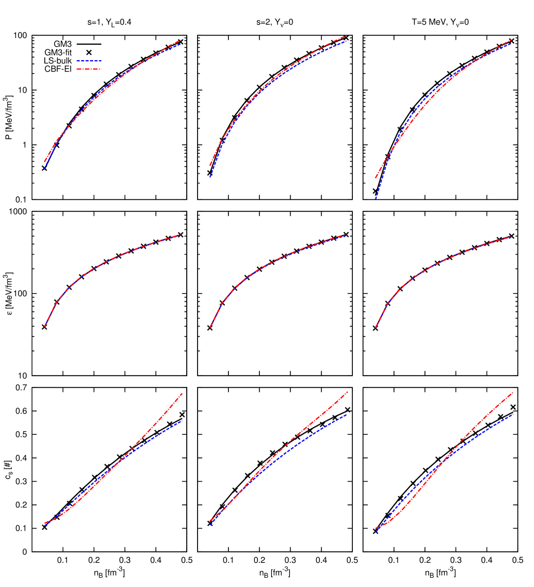
Figure 2.6: Comparison between the pressure (upper row), the energy density (middle row), and the square of the speed of sound (bottom row) for the three EoSs used in this thesis. Colors and line-styles are as in Fig. 2.4.

Conversely, after about $200\,\mathrm{ms}$ from the core bounce following a supernova explosion, the contracting core (i.e., the proto-neutron star, PNS) thermal energy is higher or comparable to the nucleons Fermi energy ($T\simeq 40\,\mathrm{MeV}\geq E_{\mathrm{F}}\simeq 30\,\mathrm{MeV}$, see Fig. 2.6) and hence one cannot use the zero temperature approximation to describe the EoS. One of the consequences is that at such high temperatures the matter EoS depends on more than one independent variable, and it is therefore called non-barotropic. In addition, in the PNS phase neutrinos are the only particles that diffuse in the star, moving energy and lepton number through the stellar layers. However, they do not leave immediately the PNS as they are produced, since at such high temperatures and densities their mean free path is far smaller than the stellar radius. The neutrino mean free path depends on the microphysical theory adopted to describe the matter; therefore, to understand the PNS evolution, one has to consistently account for the underlying EoS both to determine the PNS structure and to asses the neutrino diffusion magnitude.

In this chapter we describe and compare the three EoSs adopted in this thesis. In Sec. 2.1, we obtain several useful general and less general thermodynamic relations. In Sec. 2.2, we describe the nuclear reactions that we account for in neutrino diffusion, and we introduce the effective description of the baryon single particle spectra, which permit to include the microphysical effects of interaction in the determination of the neutrino mean free path in a general way (i.e., it may be applied to any EoS). In the following three sections we describe the three EoSs that we consider in this thesis. In Sec. 2.3 we describe the LS-bulk EoS (corresponding to the bulk of Lattimer and Swesty,, 1991), which is obtained from the extrapolation of the nuclear properties of terrestrial nuclei at high temperature and density. In Sec. 2.4 we describe the GM3 mean-field EoS (Glendenning and Moszkowski,, 1991). In Sec. 2.5 we present a many-body EoS based on the correlated basis function and the effective interaction theory (CBF-EI EoS, see Benhar and Lovato,, 2017; and Lovato et al., ming, forthcoming). In Sec. 2.6 we develop a general fitting formula for the baryon part of the EoS, that can be used to speed up the determination of the thermodynamical quantities inside the star. This fitting formula is the main original contribution presented in this chapter, and it is reported also in Camelio et al., (2017). In Sec. 2.7 we explain how to obtain the total EoS from the fitting formula for the baryon part of the EoS. Finally, in Sec. 2.8 we compare the thermodynamical quantities, the mean free paths and the diffusion coefficients of the three EoSs described in this chapter.

In this thesis, the particle energies and chemical potentials are defined including the rest mass. The (total) EoSs we consider are composed by protons, neutrons, electrons, positrons, and neutrinos and antineutrinos of all three flavours.

2.1 Thermodynamical relations

In this section we enunciate and discuss some useful thermodynamical relations, that will be used later in this thesis.

The first principle of the thermodynamics states that the variation of the energy $E$ of a system is given by

$$\mathrm{d}E=T\mathrm{d}S-P\mathrm{d}V+\sum_{i}\mu_{i}\mathrm{d}N_{i},$$ (2.1)

where $T$ is the temperature, $S$ the total entropy, $P$ the pressure, $V$ the volume, and $\mu_{i}$ and $N_{i}$ the chemical potential and total number of the particle $i$. Therefore, the most natural choice for the independent variables on which the energy depends is $E=E(S,V,\{N_{i}\})$ and

$$T={} \left.\frac{\partial E}{\partial S}\right|_{V,\{N_{i}\}},$$ (2.2)

$$P={} \left.-\frac{\partial E}{\partial V}\right|_{S,\{N_{i}\}},$$ (2.3)

$$\mu_{i}={} \left.\frac{\partial E}{\partial N_{i}}\right|_{V,S,\{N_{j\neq i}\}}.$$ (2.4)

One can define the free energy by means of a Legendre transformation:

$$F=E-TS,$$ (2.5)

and therefore,

$$\mathrm{d}F={} -S\mathrm{d}T-P\mathrm{d}V+\sum_{i}\mu_{i}\mathrm{d}N_{i},$$ (2.6)

$$F={} F(T,V,\{N_{i}\}),$$ (2.7)

$$S={} \left.-\frac{\partial F}{\partial T}\right|_{V,\{N_{i}\}},$$ (2.8)

$$P={} \left.-\frac{\partial F}{\partial V}\right|_{T,\{N_{i}\}},$$ (2.9)

$$\mu_{i}={} \left.\frac{\partial F}{\partial N_{i}}\right|_{V,T,\{N_{j\neq i}\}}.$$ (2.10)

In a stellar system, the total number of baryons is very big $A\simeq 10^{57}$, and moreover the intensive quantities (pressure, temperature, and chemical potential) change from point to point inside the star. Therefore, it is more natural to introduce the average of the extensive thermodynamical quantities at a certain point of the star. To do so, one should average over an amount of particles which is big enough to permit a statistical description of their properties, but whose extent is far smaller than the stellar scale length (e.g., the pressure scale height). In this context, it is useful to consider the average thermodynamical quantities per baryon, since the number of baryons is conserved by all type of microphysical interactions. This approach is equivalent to consider a system with a fixed number of baryons $N_{\mathrm{B}}$. The first law of the thermodynamics becomes

$$\mathrm{d}e={} T\mathrm{d}s+\frac{P}{n_{\mathrm{B}}^{2}}\mathrm{d}n_{\mathrm{B}}+\sum_{i}\mu_{i}\mathrm{d}Y_{i}\qquad \mbox{$N_{\mathrm{B}}$ constant},$$ (2.11)

$$f={} e-Ts\qquad \mbox{$N_{\mathrm{B}}$ constant},$$ (2.12)

$$\mathrm{d}f={} -s\mathrm{d}T+\frac{P}{n_{\mathrm{B}}^{2}}\mathrm{d}n_{\mathrm{B}}+\sum_{i}\mu_{i}\mathrm{d}Y_{i}\qquad \mbox{$N_{\mathrm{B}}$ constant},$$ (2.13)

$$T={} \left.\frac{\partial e}{\partial s}\right|_{n_{\mathrm{B}},\{Y_{i}\}}\qquad \mbox{$N_{\mathrm{B}}$ constant},$$ (2.14)

$$s={} \left.-\frac{\partial f}{\partial T}\right|_{n_{\mathrm{B}},\{Y_{i}\}}\qquad \mbox{$N_{\mathrm{B}}$ constant},$$ (2.15)

$$P={} \left.n_{\mathrm{B}}^{2}\frac{\partial e}{\partial n_{\mathrm{B}}}\right|_{s,\{Y_{i}\}}=\left.n_{\mathrm{B}}^{2}\frac{\partial f}{\partial n_{\mathrm{B}}}\right|_{T,\{Y_{i}\}}\qquad \mbox{$N_{\mathrm{B}}$ constant},$$ (2.16)

$$\mu_{i}={} \left.\frac{\partial f}{\partial Y_{i}}\right|_{T,n_{\mathrm{B}},\{Y_{j\neq i}\}}=\left.\frac{\partial e}{\partial Y_{i}}\right|_{s,n_{\mathrm{B}},\{Y_{j\neq i}\}}\qquad \mbox{$N_{\mathrm{B}}$ constant},$$ (2.17)

where $e=E/N_{\mathrm{B}}$, $f=F/N_{\mathrm{B}}$, $s=S/N_{\mathrm{B}}$, and $Y_{i}=N_{i}/N_{\mathrm{B}}$ are the energy per baryon, the free energy per baryon, the entropy per baryon, and the number of particle $i$ per baryon (that is also called particle number fraction, particle fraction, or particle abundance), respectively. The $i$-th particle number density is $n_{i}=N_{i}/V$, and the baryon number density is $n_{\mathrm{B}}=N_{\mathrm{B}}/V\equiv n_{p}+n_{n}$ (if the only baryons are protons and neutrons).

Eqs. (2.11) and (2.13) suggest that the energy and the free energy per baryon may be written as $e=e(s,n_{\mathrm{B}},\{Y_{i}\})$ and $f=f(T,n_{\mathrm{B}},\{Y_{i}\})$. However, the number fractions are not totally independent from each other. In fact, having fixed the baryon number implies that $\mathrm{d}Y_{p}=-\mathrm{d}Y_{n}$ (in an EoS where the only baryons are neutrons and protons). Moreover, in a realistic EoS, there are additional relations between the number fractions $Y_{i}$ (see below). Therefore, it is impossible to differentiate with respect to $Y_{p}$ (or $Y_{n}$), fixing at the same time $n_{\mathrm{B}}=n_{n}+n_{p}$ and $Y_{n}$ (or $Y_{p}$). In this case, one can consider the average thermodynamical quantities in a given volume $V$ (that is, one can fix the volume), and rewrite Eqs. (2.1) and (2.6) as

$$\mathrm{d}\epsilon={} T\mathrm{d}\sigma+\sum_{i}\mu_{i}\mathrm{d}n_{i}\qquad \mbox{$V$ constant},$$ (2.18)

$$\mathrm{d}\varphi={} -\sigma\mathrm{d}T+\sum_{i}\mu_{i}\mathrm{d}n_{i} \mbox{$V$ constant},$$ (2.19)

where $\epsilon=E/V$, $\varphi=F/V$, and $\sigma=S/V$ are the energy density, the free energy density, and the entropy density, respectively. Since $n_{\mathrm{B}}=N_{\mathrm{B}}/V$, we can also write the densities as $\epsilon=n_{\mathrm{B}}e$, $\varphi=n_{\mathrm{B}}f$, and $\sigma=n_{\mathrm{B}}s$ (beware that fixing the volume $V$ is not equivalent of fixing the baryon number in that volume, and therefore is not equivalent of fixing $n_{\mathrm{B}}$). From Eqs. (2.18) and (2.19), one obtains the chemical potential of the $i$-th species

$$\mu_{i}=\left.\frac{\partial(n_{\mathrm{B}}f)}{\partial n_{i}}\right|_{T,\{n_{j\neq i}\}}=\left.\frac{\partial(n_{\mathrm{B}}e)}{\partial n_{i}}\right|_{s,\{n_{j\neq i}\}}.$$ (2.20)

There is another important relation that is worth introducing before specialize the discussion to the stellar case. One can write Eq. (2.1) in terms of $E=V\epsilon$, $S=V\sigma$, $N_{i}=Vn_{i}$, without fixing the volume or the baryon number,

$$\epsilon\mathrm{d}V+V\mathrm{d}\epsilon={} T\sigma\mathrm{d}V+TV\mathrm{d}\sigma-P\mathrm{d}V+\sum_{i}\big{(}\mu_{i}n_{i}\mathrm{d}V+\mu_{i}V\mathrm{d}n_{i}\big{)},$$ (2.21)

$$\mathrm{d}\epsilon={} T\mathrm{d}\sigma+\sum_{i}\mu_{i}\mathrm{d}n_{i}+\left(-\epsilon-P+T\sigma+\sum_{i}\mu_{i}n_{i}\right)\frac{\mathrm{d}V}{V},$$ (2.22)

and if the system is scale invariant, that is, if $\partial\epsilon/\partial V=0$, then

$$\epsilon+P=T\sigma+\sum_{i}\mu_{i}n_{i}.$$ (2.23)

Eq. (2.23) may be applied to the whole particle system, or to the subsystem made up only by particles $i$; moreover, we may redo the discussion using the quantities per baryon instead of the quantities per unit volume, obtaining an analogous relation.

In real matter the abundances $\{Y_{i}\}$ and their variations $\{\mathrm{d}Y_{i}\}$ are related to each other. For example, we have already discussed that one cannot differentiate $f$ with respect to $Y_{p}$ keeping at the same time $n_{\mathrm{B}}$ and $Y_{n}$ fixed. This is due to the definition of $n_{\mathrm{B}}$, that implies

$$Y_{p}={} 1-Y_{n}\qquad\mbox{definition of $n_{\mathrm{B}}$}.$$ (2.24)

$$\mathrm{d}Y_{p}={} -\mathrm{d}Y_{n}\qquad\mbox{(differential of the) definition of $n_{\mathrm{B}}$}.$$ (2.25)

Similarly, the charge neutrality of matter is equivalent (if the only charged particles are protons and electrons) to

$$Y_{e^{-}}=Y_{p}\qquad\mbox{charge neutrality},$$ (2.26)

which imply (but is not implied) by the request of charge conservation

$$\mathrm{d}Y_{e^{-}}=\mathrm{d}Y_{p}\qquad\mbox{charge conservation}.$$ (2.27)

Using Eqs. (2.25) and (2.27) one obtains (in an EoS with protons, neutrons, and electrons)

$$\mathrm{d}f={} -s\mathrm{d}T+\frac{P}{n_{\mathrm{B}}^{2}}\mathrm{d}n_{\mathrm{B}}+(\mu_{p}+\mu_{e^{-}}-\mu_{n})\mathrm{d}Y_{p},$$ (2.28)

$$\left.\frac{\partial f}{\partial Y_{p}}\right|_{T,n_{\mathrm{B}}}={} \mu_{p}+\mu_{e^{-}}-\mu_{n}.$$ (2.29)

We remark the difference of Eq. (2.29) with respect to Eqs. (2.17) and (2.20): in Eq. (2.29) $n_{\mathrm{B}}$ is kept constant, while the number fractions $\mathrm{d}Y_{i\neq p}$ cannot be independently fixed because they are related to each other.

The nuclear theory adds further constraints to the thermodynamical relations. We have already stated charge conservation, Eq. (2.27). If the matter is in equilibrium with respect to one nuclear reaction, for example neutrino emission/absorption (i.e., beta-equilibrium),

$$p+e^{-}\rightleftharpoons n+\nu_{e},$$ (2.30)

the chemical potentials of the corresponding particles are simply related to each other, for example (for the case of beta-equilibrium)

$$\mu_{p}+\mu_{e^{-}}=\mu_{n}+\mu_{\nu_{e}}.$$ (2.31)

To obtain Eq. (2.31), one first notices that the structure of Reaction (2.30) implies that exactly one neutron and one neutrino are produced from exactly one proton and one electron,

$$\mathrm{d}Y_{p}=\mathrm{d}Y_{e^{-}}=-\mathrm{d}Y_{n}=-\mathrm{d}Y_{\nu_{e}}.$$ (2.32)

If we assume that the reaction occurs at constant temperature and volume (i.e., the matter temperature and baryon density do not change during the reaction timescale), the free energy changes by the amount

$$\mathrm{d}f=(\mu_{p}+\mu_{e^{-}}-\mu_{n}-\mu_{\mu_{e}})\mathrm{d}Y_{p},$$ (2.33)

and since at equilibrium the free energy is at a minimum,

$$\left.\frac{\partial f}{\partial Y_{p}}\right|_{T,n_{\mathrm{B}}}\equiv 0\qquad\mbox{at equilibrium},$$ (2.34)

one finally obtains Eq. (2.31). In general,

$$\sum_{i\in\mbox{reaction}}\mu_{i}\mathrm{d}Y_{i}=0.$$ (2.35)

Similarly, we can consider the following reactions (electron-positron annihilation)

$$e^{+}+e^{-}\rightleftharpoons{} \gamma+\gamma,$$ (2.36)

$$e^{+}+e^{-}\rightleftharpoons{} \gamma+\gamma+\gamma.$$ (2.37)

First of all, we notice that if both reactions are in chemical equilibrium (as happens in the conditions present in a PNS),

$$\mu_{\gamma}=0,$$ (2.38)

from which follows

$$\mu_{e^{+}}=-\mu_{e^{-}}.$$ (2.39)

In general, the chemical potential of the antiparticle $\bar{\imath}$ is related to that of the particle $i$ by

$$\mu_{\bar{\imath}}=-\mu_{i},$$ (2.40)

if there is equilibrium with respect to the reaction of pair annihilation/creation of particle $i$. Eq. (2.40) suggests to redefine the number fractions as

$$\{Y_{i},Y_{\bar{\imath}}\}\rightarrow Y_{\imath}=Y_{i}-Y_{\bar{\imath}},$$ (2.41)

that is, to consider the net abundances of the particles. For example, for electrons and positrons, one has

$$\mu_{e}\mathrm{d}Y_{e}\equiv\mu_{e^{-}}\mathrm{d}Y_{e}=\mu_{e^{-}}(\mathrm{d}Y_{e^{-}}-\mathrm{d}Y_{e^{+}})=\mu_{e^{-}}\mathrm{d}Y_{e^{-}}+\mu_{e^{+}}\mathrm{d}Y_{e^{+}}.$$ (2.42)

In the following, unless explicitly stated and apart from neutrons and protons, we will use the notation expressed in Eq. (2.41), that is, electrons and neutrinos abundances are defined subtracting their antiparticle abundances.

We now derive a relation that will be useful in Chapter 3. We consider an EoS with protons, neutrons, electrons, positrons, and neutrinos. We include all neutrino flavours, but we will assume that muon and tauon neutrinos have vanishing chemical potential. Finally, we assume beta-equilibrium. We obtain

$$\sum_{i}\mu_{i}\mathrm{d}Y_{i}=\mu_{p}\mathrm{d}Y_{p}+\mu_{n}\mathrm{d}Y_{n}+\mu_{e}\mathrm{d}Y_{e}+\mu_{\nu_{e}}\mathrm{d}Y_{\nu_{e}}=\\ =(\mu_{p}-\mu_{n}+\mu_{e})\mathrm{d}Y_{e}+\mu_{\nu_{e}}\mathrm{d}Y_{\nu_{e}}=\mu_{\nu_{e}}\mathrm{d}(Y_{e}+Y_{\nu})=\mu_{\nu_{e}}\mathrm{d}Y_{\mathrm{L}_{e}},$$ (2.43)

where we have used Eqs. (2.25), (2.27), and (2.31). We observe that Eq. (2.43) may seem in contrast with Eq. (2.35) and the request of beta-equilibrium. This apparent paradox arises because we have not used Eq. (2.32), that is, the number fraction variations do not respect the stoichiometry of the beta-equilibrium reaction even though the chemical potentials are derived from beta-equilibrium. This is due to the fact that in deriving Eq. (2.43) we are implicitly interested in the process of neutrino diffusion in the star, which has a timescale longer than that of beta-equilibrium (see Appendix B). Therefore, since beta-equilibrium is respected on these timescales, the relation between chemical potentials due to beta-equilibrium still holds [Eq. (2.31)], but Eq. (2.32) is not valid on these timescales since the neutrino number change is due to a process different from beta-equilibrium (i.e., neutrino diffusion). Charge conservation [Eq. (2.27)] is still valid since baryons and electrons are locked on the timescales of PNS evolution: only neutrinos diffuse through the star.

2.2 Baryons effective spectra and neutrino diffusion

In a PNS the massive particles are locked, that is, they cannot diffuse. Therefore, energy and composition (i.e., the number fractions $Y_{i}$) changes are driven only by neutrino diffusion, since we neglect the contribution of photons. To consistently determine how the PNS evolves, it is therefore fundamental to determine the neutrino cross sections in high density, finite temperature matter. In this section we describe how we have treated neutrino diffusion consistently with the underlying EoS.

As we explain in Chapter 3, the diffusion coefficients $D_{2}$, $D_{3}$, and $D_{4}$ employed in the PNS evolution are (Pons et al.,, 1999; all non-electronic neutrinos are treated as muon neutrinos)

$$D_{2}={} D_{2}^{\nu_{e}}+D_{2}^{\bar{\nu}_{e}},$$ (2.47)

$$D_{3}={} D_{3}^{\nu_{e}}-D_{3}^{\bar{\nu}_{e}},$$ (2.48)

$$D_{4}={} D_{4}^{\nu_{e}}+D_{4}^{\bar{\nu}_{e}}+4D_{4}^{\nu_{\mu}},$$ (2.49)

$$D^{\nu_{i}}_{n}={} \int_{0}^{\infty}\mathrm{d}xx^{n}\lambda_{\mathrm{tot}}^{\nu_{i}}(\omega)f^{\nu_{i}}(\omega)\big{(}1-f^{\nu_{i}}(\omega)\big{)},$$ (2.50)

$$\frac{1}{\lambda^{\nu_{i}}_{\mathrm{tot}}(\omega)}={} \sum_{j\in\{\mathrm{reactions\}}}\frac{\sigma_{j}^{\nu_{i}}(\omega)}{V},$$ (2.51)

where $f^{\nu_{i}}(\omega)$, $\lambda_{\mathrm{tot}}^{\nu_{i}}(\omega)$, and $\sigma_{j}^{\nu_{i}}$ are the distribution function, the total mean free path, and the cross-section of a $\nu_{i}$ neutrino of energy $\omega=xT$ and each quantity depends on the temperature and the particle chemical potentials, which are determined by the underlying EoS.

The nuclear processes that we consider in Eq. (2.51) are the scattering of all neutrino types on electrons, protons, and neutrons and the absorption of electron neutrino and electron anti-neutrino on neutron and proton, respectively, with their inverse processes (for details regarding the inverse processes, see Appendix C)

$$\nu_{i}+n\rightleftharpoons{} \nu_{i}+n,$$ (2.52)

$$\nu_{i}+p\rightleftharpoons{} \nu_{i}+p,$$ (2.53)

$$\nu_{i}+e^{-}\rightleftharpoons{} \nu_{i}+e^{-},$$ (2.54)

$$\nu_{e}+n\rightleftharpoons{} e^{-}+p,$$ (2.55)

$$\bar{\nu}_{e}+p\rightleftharpoons{} e^{+}+n.$$ (2.56)

To determine the cross-sections $\sigma(E)$ we use Eq. (82) of Reddy et al., (1998); the coupling constants for the different reactions are reported in Reddy et al., (1998, Tabs. I and II). In order to compute the neutrino scattering and absorption cross-sections on interacting baryons, Reddy et al., (1998) make use of the baryon effective parameters (effective masses and single particle potentials, see below), that allow to approximate the relativistic single particle spectra of the interacting baryons. The use of the single particle spectrum approximation is applicable only when it is reasonable to describe matter in terms of quasi-particles, that is, near the Fermi surface. This approximation is justified since, due to the Pauli blocking effect, neutrinos may interact only with baryons near their Fermi surface. To compute the diffusion coefficients in a point of the star, we need therefore to determine the approximated baryon effective spectra corresponding to the thermodynamical conditions in that point of the star.

The spectrum of a free relativistic particle $\mathcal{E}^{K}(k)$ is given by its kinetic energy

$$\mathcal{E}^{K}(k)=\sqrt{k^{2}+m^{2}},$$ (2.57)

where $m$ is the particle mass. The interaction between particles changes the single-particle spectrum, $\mathcal{E}(k)$. One can effectively describe the single particle spectrum introducing the particle effective mass $m^{\ast}$ and the single particle potential $U$,

$$\mathcal{E}(k)\simeq\sqrt{k^{2}+m^{\ast}{}^{2}}+U.$$ (2.58)

Eq. (2.58) is exact in the case of a mean-field EoSs [like GM3, see Sec. 2.4, in particular Eq. (2.92)], and it is only approximate for a more realistic EoS, like a many-body EoS (see discussion in Sec. 2.5). This is due to the fact that, in the many-body formalism, the concept of single particle is not well-posed; moreover, assuming that it is possible to define a single-particle spectrum, it is only approximately given by Eq. (2.58). As a consequence, the thermodynamical quantities ($f$, $s$, $P$, and so on) are only approximately recovered by integrating the effective spectra of protons and neutrons (that is, by inserting the effective masses and single particle potentials in the Fermi gas expressions, as done in Eqs. (2.4) and (2.97) for the GM3 EoS). This is expected and is not a relevant issue; in fact, in our work the effective masses and single particle potentials are used only to compute the diffusion coefficients and not the other EoS quantities, for which we have performed a different fit (see Secs. 2.6 and 2.7), and therefore there are no consistency problems. On the contrary, it is important to recover the baryon densities $n_{n}$ and $n_{p}$ from the effective spectrum description (as done in Eqs. (2.86) for the GM3 EoS), since the mean free paths are “intensive” quantities, Eq. (2.51). If the baryon densities are poorly recovered from the effective spectrum description, one is erroneously using diffusion coefficients at baryon density $n_{\mathrm{B}}$ and proton fraction $Y_{p}$, while they would correspond to those at baryon density $n_{\mathrm{B}}^{\prime}$ and proton fraction $Y_{p}^{\prime}$, compromising the consistency of the PNS evolution. To be more explicit,

$$n_{i}=\frac{4\pi}{h^{3}}\int\frac{p^{2}\mathrm{d}p}{1+\mathrm{e}^{\frac{\sqrt{p^{2}+m^{2}}-\mu_{i}^{K}}{T}}}\simeq\frac{4\pi}{h^{3}}\int\frac{p^{2}\mathrm{d}p}{1+\mathrm{e}^{\frac{\sqrt{p^{2}+m^{\ast 2}}+U_{i}-\mu_{i}}{T}}},$$ (2.59)

where $\mu_{i}^{K}$ is the chemical potential of a free Fermi gas with the same baryon density $n_{\mathrm{B}}$, temperature $T$, and proton fraction $Y_{p}$ of the interacting Fermi gas. The raison d’être of Eq. (2.59) will become clear in Secs. 2.6 and 2.7, here we anticipate that to determine the total EoS we consider first the non-interacting baryon EoS, whose density, temperature and proton fraction are the same of the total interacting baryon EoS. Eq. (2.59) is a consequence of this procedure and of the request that the baryon densities recovered by the effective spectra are as those given by the EoS.

In the PNS evolution code the neutrino diffusion coefficients are evaluated by linear interpolation of a three-dimensional table, evenly spaced in $Y_{\nu}$ (the neutrino number fraction), $T$, and $n_{\mathrm{B}}$. The table has been produced consistently with the underlying EoS. To generate the table, we have first solved the EoS using the method described in Sec. 2.7, obtaining the particles chemical potentials. The proton and neutron effective masses and single particle potentials have been obtained by linear interpolation of a table evenly spaced in $Y_{p}$, $T$, and $n_{\mathrm{B}}$. The neutrino cross sections (Eq. (82) of Reddy et al.,, 1998) and the neutrino diffusion coefficients [Eq. (2.50)] have been integrated by Gaussian quadrature.

2.3 An extrapolated baryon EoS: LS-bulk

In this section we describe a high density EoS obtained from the extrapolation of the properties of nuclear matter obtained by experiments on terrestrial nuclei. In particular, this EoS has been used by Lattimer and Swesty, (1991) for the bulk nuclear matter, that is, baryons are treated as an interacting gas of protons and neutrons (there are neither alpha particles, pasta phases, nor lattice). We call this EoS LS-bulk.

The well-known semi-empirical formula of the nuclear binding energy permits to fit with a few parameters the binding energy of terrestrial nuclei with an astonishing precision (Krane,, 1987)

$$E(N_{p}\equiv Z,N_{\mathrm{B}}\equiv A)=N_{p}m_{p}+N_{n}m_{n}-a_{v}N_{\mathrm{B}}+a_{s}N_{\mathrm{B}}^{2/3}\\ +a_{c}N_{p}(N_{p}-1)N_{\mathrm{B}}^{-1/3}+a_{\mathrm{sym}}\frac{(N_{\mathrm{B}}-2N_{p})^{2}}{N_{\mathrm{B}}}-\delta a_{p}N_{\mathrm{B}}^{-3/4},$$ (2.60)

where $N_{p}\equiv Z$ and $N_{n}$ are the number of protons and neutrons in the nucleus, respectively, $N_{\mathrm{B}}=N_{p}+N_{n}\equiv A$ is the number of baryons, and $a_{v}$, $a_{s}$, $a_{c}$, $a_{\mathrm{sym}}$, and $\delta a_{p}$ (with $\delta=\{-1;0;1\}$) are parameters that assess the importance of the volume, surface, Coulomb, symmetry and pairing force terms, respectively, and whose particular value may be determined by fitting the measured masses of terrestrial nuclei (Krane,, 1987). To extrapolate a high density stellar EoS from Eq. (2.60), one considers the limit of infinite nuclear matter, retaining only the terms proportional to the volume, and adds some terms that account for other nuclear properties, like the nuclear imcompressibility. The semi-empirical formula for the free energy of infinite nuclear matter may therefore be written as (Eq. (2.3) of Lattimer and Swesty,, 1991)

$$f_{B}(T,n_{\mathrm{B}},Y_{p})=m_{n}-\mathrm{BE}-\Delta_{m}Y_{p}\\ +\frac{K_{s}}{18}\left(1-\frac{n_{\mathrm{B}}}{n_{s}}\right)^{2}+S_{v}(1-2Y_{p})^{2}-a_{T}T^{2},$$ (2.61)

where

• $\Delta_{m}\equiv m_{n}-m_{p}$ is the neutron-proton mass difference; at variance with Lattimer and Swesty, (1991) we set this term to zero;

• $n_{s}$ is the saturation density of symmetric nuclear matter, that is, the density for which

  $$\left.\frac{\partial P_{B}}{\partial n_{\mathrm{B}}}\right|_{T=0,Y_{p}=1/2}=0.$$ (2.62)

  We adopt the same value of Lattimer and Swesty, (1991), $n_{s}=0.155\,\mathrm{fm^{-3}}$.

• $\mathrm{BE}=-f_{B}(T=0,n_{s},Y_{p}=1/2)-\Delta_{m}/2\equiv a_{v}$ is the binding energy of saturated, symmetric nuclear matter. Its value can be derived from nuclear mass fits; we set it to the same value of Lattimer and Swesty, (1991), $\mathrm{BE}=16\,\mathrm{MeV}$.

• $K_{s}$ is the imcompressibility of bulk nuclear matter,

  $$K_{s}=\left.9n_{\mathrm{B}}^{2}\frac{\partial^{2}f_{B}}{\partial n_{\mathrm{B}}^{2}}\right|_{T=0,n_{\mathrm{B}}=n_{s},Y_{p}=1/2}.$$ (2.63)

  $K_{s}$ can be determined by isoscalar breathing modes and isotopic differences in charge densities of large nuclei. At variance with Lattimer and Swesty, (1991), we take $K_{s}=220\,\mathrm{MeV}$, a value which is more similar to recent measurements and to those of the other EoSs we are considering.

• $S_{v}$ is the symmetry energy parameter of bulk nuclear matter,

  $$S_{v}=\left.\frac{1}{8}\frac{\partial^{2}f_{\mathrm{B}}}{\partial Y_{p}^{2}}\right|_{T=0,n_{\mathrm{B}},Y_{p}=1/2}\equiv a_{\mathrm{sym}},$$ (2.64)

  it can be derived from the fit of the mass formula and from giant dipole resonances; as Lattimer and Swesty, (1991) we set its value to $S_{v}=29.3\,\mathrm{MeV}$.

• $a_{T}$ is the bulk level density parameter,

  $$a_{T}=-\left.\frac{1}{2}\frac{\partial^{2}f_{\mathrm{B}}}{\partial^{2}T}\right|_{T=0,n_{\mathrm{B}},Y_{p}=1/2}\simeq\frac{1}{15}\frac{m^{\ast}}{m_{n}}\mathrm{MeV^{-1}},$$ (2.65)

  and it is related to the nucleon effective mass $m^{\ast}$. However, following Lattimer and Swesty, (1991), we set the effective masses of protons and neutrons for the LS-bulk EoS equal to their rest masses; and in addition the thermal contribution to the LS-bulk EoS is given only by the kinetic term (see below). Therefore the parameter $a_{T}$ is not relevant to the following discussion.

With this choice of parameters, we obtain a maximum mass for a non-rotating cold star of $M_{\mathrm{LSbulk}}\simeq 2.02\,\mathrm{M_{\odot}}$ (Camelio et al.,, 2017).

Lattimer and Swesty, (1991) give the following parametrization for the baryon free energy at finite temperature

$$f_{\mathrm{B}}(T,n_{\mathrm{B}},Y_{p})={} f_{\mathrm{B}}^{K}(T,n_{\mathrm{B}},Y_{p})+f_{\mathrm{B}}^{I}(T,n_{\mathrm{B}},Y_{p}),$$ (2.66)

$$f_{\mathrm{B}}^{I}(T,n_{\mathrm{B}},Y_{p})={} \big{(}a+4bY_{p}(1-Y_{p})\big{)}n_{\mathrm{B}}+cn_{\mathrm{B}}^{\delta}-Y_{p}\Delta_{m},$$ (2.67)

where $f_{\mathrm{B}}^{K}$ is the free energy per baryon of a free gas of protons and neutrons, but with the same baryon density, temperature, and proton fraction of the total interacting baryon free energy, and $f_{\mathrm{B}}^{I}$ is the interacting contribution to the free energy. The proton-neutron mass difference can appears only in the interaction term, while in the kinetic term proton and neutrons have the same mass. To obtain the values of the parameters in Eq. (2.67), one should take the expression for the interacting free energy [Eq. (2.61)] at zero temperature and subtract the (non-relativistic) zero temperature non-interacting contribution, $f_{\mathrm{B}}^{K}$, see Appendix A.2. One obtains (Eq. (2.21) of Lattimer and Swesty,, 1991; beware that Eq. (2.19c) of Lattimer and Swesty,, 1991 has a typo)

$$\alpha={} \frac{3\hbar^{2}}{10m_{n}}(3\pi^{2}n_{s}/2)^{2/3},$$ (2.68)

$$\delta={} \frac{K_{s}+2\alpha}{3\alpha+9\mathrm{BE}}=1.260,$$ (2.69)

$$b={} \frac{\alpha(2^{2/3}-1)-S_{v}}{n_{s}}=-107.1\,\mathrm{MeV\,fm^{3}},$$ (2.70)

$$a={} \frac{\delta(\alpha+\mathrm{BE})-2\alpha/3}{n_{s}(1-\delta)}-b=-711.0\,\mathrm{MeV\,fm^{3}},$$ (2.71)

$$c={} \frac{K_{s}+2\alpha}{9\delta(\delta-1)n_{s}^{\delta}}=934.6\,\mathrm{MeV\,fm^{3\delta}},$$ (2.72)

$$\Delta_{m}={} 0,$$ (2.73)

where we set the effective masses of protons and neutrons equal to the rest mass of neutrons, $m^{\ast}=m_{n}$, and $\alpha$ is the internal energy (i.e., the energy without the contribution of the bare rest mass $m_{n}$) of a non-relativistic free gas of protons and neutrons at $T=0$, $n_{\mathrm{B}}=n_{s}$, and $Y_{p}=1/2$. Since we have not considered thermal effects in the determination of the interacting contribution to the free energy, those are included in the LS-bulk EoS only by the kinetic term, $f_{\mathrm{B}}^{K}$.

As we have discussed in Sec. 2.2, it is important that the baryon densities recovered from the effective single particle spectra are equal to the densities obtained solving the EoS. Since for the LS-bulk we have set $m^{\ast}_{i}=m_{n}$, this means that [see Eq. (2.59)]

$$U_{i}=\mu^{I}_{i}=\mu_{i}-\mu_{i}^{K},$$ (2.74)

where $\mu_{i}^{I}$ and $\mu^{K}_{i}$ are the kinetic and interacting parts of the chemical potential, obtained by differentiating the kinetic $f^{K}_{\mathrm{B}}$ and interacting $f^{I}_{\mathrm{B}}$ parts of the free energy, see Eqs. (2.66) and (2.20), and the index refers to protons and neutrons, $i\in\{p,n\}$.

2.4 A mean-field baryon EoS: GM3

At the center of a neutron star, the baryon density may easily reach 4 or 5 times the nuclear saturation density, $n_{s}$. At such high densities, the Fermi momentum is expected to be comparable to the baryon masses ($k_{\mathrm{F}n}\simeq 450\,\mathrm{MeV}$ at $n_{n}\simeq 0.4\,\mathrm{fm^{-3}}$, and $m_{n}\simeq 939\,\mathrm{MeV}$), and therefore it would be preferable to adopt a relativistic description of baryons (Prakash et al.,, 1997). In the following, we consider a model (Walecka,, 1974; Glendenning,, 1985) where the nuclear forces between baryons are mediated by the exchange of the $\sigma$, $\rho$, and $\omega$ mesons. This model is easily extended with the presence of hyperons; however we do not include them because the other EoSs considered in this thesis (LS-bulk and CBF-EI) are composed only by protons and neutrons. To simplify the notation, in this section we set $\hbar=c=1$.

The baryon Lagrangian is (Glendenning,, 1985; Prakash et al.,, 1997)

$$\mathcal{L}_{\mathrm{B}}=\sum_{i\in\{p,n\}}\bar{\psi}_{i}(\imath\gamma^{\mu}\partial_{\mu}-g_{\omega i}\gamma^{\mu}\omega_{\mu}-g_{\rho i}\gamma^{\mu}\vec{\rho}_{\mu}\cdot\vec{t}-m_{i}+g_{\sigma i}\sigma)\psi_{i}\\ +\frac{1}{2}\partial_{\mu}\sigma\partial^{\mu}\sigma-\frac{1}{2}m_{\sigma}^{2}\sigma^{2}-U(\sigma)-\frac{1}{4}W_{\mu\nu}W^{\mu\nu}+\frac{1}{2}m_{\omega}^{2}\omega_{\mu}\omega^{\mu}\\ -\frac{1}{4}\vec{R}_{\mu\nu}\cdot\vec{R}^{\mu\nu}+\frac{1}{2}m_{\rho}^{2}\vec{\rho}_{\mu}\cdot\vec{\rho}^{\mu},$$ (2.75)

where $\psi_{i}=\psi_{i}(x)$ is the wave function of the proton or the neutron, $\sigma=\sigma(x)$, $\omega_{\mu}=\omega_{\mu}(x)$ and $\vec{\rho}_{i}=\vec{\rho}_{i}(x)$ are the meson wave functions, $W_{\mu\nu}=\partial_{\mu}\omega_{\nu}-\partial_{\nu}\omega_{\mu}$, $\vec{R}_{\mu\nu}=\partial_{\mu}\vec{\rho}_{\nu}-\partial_{\nu}\vec{\rho}_{\nu}$, $g_{ji}$ are the coupling constants between the meson $j$ and the baryon $i$, $\vec{t}$ is the baryon isospin operator and the potential

$$U(\sigma)=(bm_{n}+cg_{\sigma}\sigma)(g_{\sigma}\sigma)^{3}$$ (2.76)

represents the self-interaction of the $\sigma$ field ($b$, $c$ and $g_{\sigma}$ are parameters).

With Glendenning, (1985), we define the normal state of infinite matter as “uniform and isotropic, and […] the baryon eigenstates in the medium carry the same quantum numbers as they do in vacuum” (Glendenning,, 1985). In addition, we apply the mean-field approximation, that is, we replace the meson fields by their mean values, $\sigma(x)\rightarrow\sigma$, $\omega_{\mu}(x)\rightarrow\omega_{\mu}$, and $\vec{\rho}_{\mu}(x)\rightarrow\vec{\rho}_{\mu}$.

We remind that the Euler-Lagrange equation for the field $\psi$ is

$$\partial_{\mu}\left(\frac{\partial\mathcal{L}}{\partial(\partial_{\mu}\psi)}\right)=\frac{\partial\mathcal{L}}{\partial\psi}.$$ (2.77)

Evaluating Eq. (2.77) for the meson fields we obtain (since the field wave functions are constants in the mean-field approximation, the spatial derivatives vanish)

$$m_{\sigma}^{2}\sigma={} -\frac{\mathrm{d}U(\sigma)}{\mathrm{d}\sigma}+\sum_{i\in\{p,n\}}g_{\sigma i}<\bar{\psi}_{i}\psi_{i}>,$$ (2.78)

$$m_{\omega}^{2}\omega^{\mu}={} \sum_{i\in\{p,n\}}g_{\omega i}<\bar{\psi}_{i}\gamma^{\mu}\psi_{i}>,$$ (2.79)

$$m_{\rho}^{2}\rho_{1}^{\mu}={} \frac{1}{2}\big{(}g_{\rho p}<\bar{\psi}_{p}\gamma^{\mu}\psi_{n}>+g_{\rho n}<\bar{\psi}_{n}\gamma^{\mu}\psi_{p}>\big{)}=0,$$ (2.80)

$$m_{\rho}^{2}\rho_{2}^{\mu}={} \frac{1}{2}\big{(}-\imath g_{\rho p}<\bar{\psi}_{p}\gamma^{\mu}\psi_{n}>+\imath g_{\rho n}<\bar{\psi}_{n}\gamma^{\mu}\psi_{p}>\big{)}=0,$$ (2.81)

$$m_{\rho}^{2}\rho_{3}^{\mu}={} \sum_{i\in\{p,n\}}g_{\rho i}t_{3i}<\bar{\psi}_{i}\gamma^{\mu}\psi_{i}>,$$ (2.82)

where the third component of the isospin is $t_{3p}=+1/2$ for the proton and $t_{3n}=-1/2$ for the neutron. The expectation value of the charged $\rho$ mesons vanishes since in nuclear normal matter baryons carry the same quantum numbers as they do in vacuum, and the first two isospin operators change the isospin of the wavefunction they are applied to [flip protons in neutrons, see Eqs. (2.80) and (2.81)]. Moreover, since nuclear normal matter is isotropic, the expectation value of $<\bar{\psi}\gamma^{i}\psi>$, with $i=\{1,2,3\}$, vanishes (Walecka,, 1974), and therefore

$$m_{\omega}^{2}\omega^{0}={} \sum_{i\in\{p,n\}}g_{\omega i}<\bar{\psi}_{i}\gamma^{0}\psi_{i}>,$$ (2.83)

$$m_{\rho}^{2}\rho_{3}^{0}={} \sum_{i\in\{p,n\}}g_{\rho i}t_{3}<\bar{\psi}_{i}\gamma^{0}\psi_{i}>,$$ (2.84)

$$\omega^{j}={} \rho_{3}^{j}=0,$$ (2.85)

where $n_{i}$ is the density of the baryon $i$ and $j$ is a spatial index. It is possible to show that (Glendenning,, 1985; Prakash et al.,, 1997)

$$<\bar{\psi}_{i}\gamma^{0}\psi_{i}>={} <\psi_{i}^{\dagger}\psi_{i}>\equiv n_{i}=4\pi\int_{0}^{\infty}f_{i}(p)p^{2}\mathrm{d}p,$$ (2.86)

$$<\bar{\psi}_{i}\psi_{i}>={} 4\pi\int_{0}^{\infty}\frac{m_{i}-g_{\sigma i}\sigma}{\sqrt{p^{2}+(m_{i}-g_{\sigma i}\sigma)^{2}}}f_{i}(p)p^{2}\mathrm{d}p,$$ (2.87)

where $f_{i}(p)$ is the distribution function of the interacting baryon $i$, Eq. (2.93), that is different from the non-interacting distribution function, see below.

Applying the Euler-Lagrange equation to the baryon fields one obtain the Dirac equations for baryons,

$$\left[\gamma^{0}(p_{0}-g_{\omega i}\omega_{0}-t_{3}g_{\rho i}\rho_{03})+\gamma^{j}p_{j}-(m_{i}-g_{\sigma i}\sigma)\right]\psi_{i}=0,$$ (2.88)

and from them the baryon spectra

$$\mathcal{E}_{i}(\vec{p})=g_{\omega i}\omega_{0}+t_{3}g_{\rho i}\rho_{03}+\sqrt{p^{2}+(m_{i}-g_{\sigma i}\sigma)^{2}}.$$ (2.89)

We notice that, defining the effective mass $m^{\ast}$ and the single particle potential $U$,

$$m^{\ast}_{i}={} m_{i}-g_{\sigma i}\sigma,$$ (2.90)

$$U_{i}={} g_{\omega i}\omega_{0}+t_{3}g_{\rho i}\rho_{03},$$ (2.91)

we can write the mean-field baryon spectra in a way that is formally identical to Eq. (2.58),

$$\mathcal{E}_{i}(p)=\sqrt{p^{2}+m_{i}^{\ast 2}}+U_{i},$$ (2.92)

where in general the effective masses and single particle potentials depend on the density and the temperature. The baryon interacting distribution function is

$$f_{i}(p)=\frac{g_{i}/h^{3}}{1+\exp\left(\frac{\mathcal{E}_{i}(k)-\mu_{i}}{T}\right)}=\frac{g_{i}/h^{3}}{1+\exp\left(\frac{\sqrt{p^{2}+m_{i}^{\ast 2}}+U_{i}-\mu_{i}}{T}\right)},$$ (2.93)

where $g_{i}$ is the baryon degeneracy (for protons and neutrons, $g_{i}=2$).

For given temperature $T$ and chemical potentials $\mu_{p}$ and $\mu_{n}$, Eqs. (2.78), (2.83), (2.84), (2.86), (2.87), (2.93) may be solved iteratively (e.g., with a Newton-Raphson algorithm) to give the mean-field values of the meson fields and the baryon effective masses and single particle potentials. From the stress-energy tensor and the partition function one can then obtain the other thermodynamical quantities (Glendenning,, 1985; Prakash et al.,, 1997). However, we find instructive to adopt here a heuristic argument to obtain the thermodynamical quantities. First of all, the contribution to the thermodynamical quantities given by the baryons may be obtained from the Eqs. (A.11) and (A.12), substituting the free baryon energy spectra with the interacting ones, Eq. (2.92). However, one has to consider also the contribution given by the meson fields. From the Lagrangian (2.75), it is apparent that the contribution at the mean-field level is

$$\epsilon_{\mathrm{mesons}}=+\frac{1}{2}m_{\sigma}^{2}\sigma^{2}+U(\sigma)-\frac{1}{2}m_{\omega}^{2}\omega_{0}^{2}-\frac{1}{2}m_{\rho}^{2}\rho_{03}^{2}.$$ (2.94)

Since the meson fields are treated at the mean-field level,

$$P_{\mathrm{mesons}}=-\epsilon_{\mathrm{mesons}}.$$ (2.95)

Then, the total baryon energy is (Prakash et al.,, 1997)

$$\epsilon_{\mathrm{B}}={} \epsilon_{\mathrm{mesons}}+\epsilon_{p}+\epsilon_{n}=+\frac{1}{2}m_{\sigma}^{2}\sigma^{2}+U(\sigma)-\frac{1}{2}m_{\omega}^{2}\omega_{0}^{2}-\frac{1}{2}m_{\rho}^{2}\rho_{03}^{2}$$

$$+4\pi\sum_{i\in\{p,n\}}\int\left(\sqrt{p^{2}+m_{i}^{\ast 2}}+U_{i}\right)f_{i}(p)p^{2}\mathrm{d}p$$

$$={} \frac{1}{2}m_{\sigma}^{2}\sigma^{2}+U(\sigma)+\frac{1}{2}m_{\omega}^{2}\omega_{0}^{2}+\frac{1}{2}m_{\rho}^{2}\rho_{03}^{2}$$

$$+4\pi\sum_{i\in\{p,n\}}\int\sqrt{p^{2}+m_{i}^{\ast 2}}f_{i}(p)p^{2}\mathrm{d}p,$$ (2.96)

where in the last step we have used Eqs. (2.91), (2.83) and (2.84). The total baryon pressure is (Prakash et al.,, 1997)

$$P_{\mathrm{B}}=P_{\mathrm{field}}+P_{p}+P_{n}=-\frac{1}{2}m_{\sigma}^{2}\sigma^{2}-U(\sigma)+\frac{1}{2}m_{\omega}^{2}\omega_{0}^{2}+\frac{1}{2}m_{\rho}^{2}\rho_{03}^{2}+P_{p}+P_{n},$$ (2.97)

and the total baryon entropy can be obtained from Eq. (2.23). We remark that the condition in Eq. (2.59) is automatically fulfilled, since by construction the baryon thermodynamical quantities are obtained from their single particle effective spectra.

In this thesis, we have adopted the set of parameters denoted as GM3 (Glendenning and Moszkowski,, 1991; Pons et al.,, 1999, see Table 2.1 of this thesis), which correspond to a saturation density $n_{s}=0.153\,\mathrm{fm^{-3}}$, a binding energy $\mathrm{BE}=16.3\,\mathrm{MeV}$, a bulk imcompressibility parameter $K_{s}=240\,\mathrm{MeV}$, and a symmetry energy $S_{v}=32.5\,\mathrm{MeV}$. The maximum mass of a cold NS with the GM3 EoS is $M_{\mathrm{GM3}}\simeq 2.02\,\mathrm{M_{\odot}}$ (Camelio et al.,, 2017).

Table 2.1: GM3 parameters (Glendenning and Moszkowski,, 1991; Pons et al.,, 1999). Since the meson couplings are the same for protons and neutrons, we drop the baryon index (e.g., $g_{\sigma p}=g_{\sigma n}\equiv g_{\sigma}$).

$g_{\sigma}/m_{\sigma}$	$3.151$	fm
$g_{\omega}/m_{\omega}$	$2.195$	fm
$g_{\rho}/m_{\rho}$	$2.189$	fm
$b$	$0.008659$	#
$c$	$-0.002421$	#

As a final remark, we notice that since $g_{\sigma p}=g_{\sigma n}$ (see Table 2.1), the effective masses of proton and neutron are the same [Eq. (2.90)]; whereas their single particle potential is different because of the presence of the third component of the isospin in Eq. (2.91). This behaviour is due to the way baryons couple to the (neutral) rho meson $\rho_{3}$ [Eqs. (2.75) and (2.84)], which therefore is responsible of the symmetry energy that drives the neutron excess in nuclear matter.

2.5 A many-body baryon EoS: CBF-EI

The mean-field approximation we have described in Sec. 2.4 consists in the assumption that meson fields may be replaced by their mean value, that is, meson wavefunctions oscillate many times on the scale length of the baryon wavefunctions. However, in a neutron star density may easily reach $n_{\mathrm{B}}\simeq 0.4\,\mathrm{fm^{-3}}$, that corresponds to an average distance between nucleons of the order of $d\simeq 1.7\,\mathrm{fm}$, which is comparable to the meson Compton wavelengths $\lambda_{\mathrm{c}}=h/m$ ($\lambda_{\sigma}=0.33\,\mathrm{fm}$, $\lambda_{\omega}=0.25\,\mathrm{fm}$, and $\lambda_{\rho}=0.26\,\mathrm{fm}$). In addition, at the mean-field level the pion meson expectation value is zero, whereas pion exchange is the main process that determines the baryon interaction. Therefore, the mean-field approximation is poorly justified in this regime. In this section we describe a non-relativistic many-body EoS that is based on the semi-phenomenological nuclear potentials Argonne $v^{\prime}_{6}$ and Urbana IX (Lovato,, 2012; Benhar and Lovato,, 2017), that takes into account aspects of the nuclear dynamics that are neglected by the mean-field approximation. This EoS is based on the correlated basis function theory and makes use of the Hartree-Fock effective interaction, and therefore we call it CBF-EI EoS.

There are strong numerical and experimental evidence that the Hamiltonian of a many body nuclear system is given by

$$\hat{H}=-\sum_{i}\frac{\nabla^{2}_{i}}{2m\hbar}+\sum_{i>j}\hat{v}_{ij}+\sum_{k>j>i}\hat{V}_{ijk},$$ (2.98)

where sums are performed over the nucleons, and $\hat{v}_{ij}$ and $\hat{V}_{ijk}$ are two- and three-body potentials. The inclusion of the additional three-nucleon term, $V_{ijk}$, is needed to explain the binding energies of three-nucleon systems and the saturation properties of symmetric neutron matter. The three-nucleon force is the consequence of having neglected the quark degrees of freedom, that is implicit in the formulation of the problem in terms of nucleons (each nucleon is composed at a more fundamental level by three quarks). Theoretical, numerical and phenomenological constraints permit to determine the form of the terms entering in the potentials $\hat{v}_{ij}$ and $\hat{V}_{ijk}$. The two-body form of the potential of the CBF-EI EoS considered in this thesis is the so called Argonne $v^{\prime}_{6}$ potential, $\hat{v}_{ij}\equiv\hat{v}^{\prime}_{6}(r_{ij})$

$$\hat{v}^{\prime}_{6}(r_{ij})={} \sum_{p=1}^{6}v^{p}(r_{ij})\hat{O}^{p}_{ij},$$ (2.99)

$$\hat{O}^{p=1-6}_{ij}={} (1,\vec{\sigma}_{i}\cdot\vec{\sigma}_{j},S_{ij})\otimes(1,\vec{\tau}_{i}\cdot\vec{\tau}_{j}),$$ (2.100)

$$S_{ij}={} \frac{3}{r_{ij}^{2}}(\vec{\sigma}_{i}\cdot\vec{r}_{ij})(\sigma_{j}\cdot\vec{r}_{ij})-(\vec{\sigma}_{i}\cdot\vec{\sigma}_{j}),$$ (2.101)

where $\sigma_{i}$ and $\tau_{i}$ are the Pauli matrices acting on the spin and isospin of particle $i$, ans $r_{ij}$ is the distance between the two particles. The CBF-EI EoS uses as three-body potential the Urbana IX potential (Fujita and Miyazawa,, 1957; Pudliner et al.,, 1995), whose expression may be found for example in Lovato, (2012).

Within the Hartree-Fock approximation, the many-body ground state is assumed to be the Slater determinant of a system of $N_{\mathrm{B}}$ interacting baryons,

$$\hat{H}\Psi_{0}(x_{1},\ldots,x_{N_{\mathrm{B}}})=E_{0}\Psi_{0}(x_{1},\ldots,x_{n_{\mathrm{B}}}),$$ (2.102)

where $\Psi_{0}(x_{1},\ldots,x_{N_{\mathrm{B}}})$ is the many-body wave eigenfunction corresponding to the energy ground state $E_{0}$. Usually in the Hartree-Fock procedure one adopts as many-body trial wavefunction the Slater determinant of $N_{\mathrm{B}}$ one-nucleon wavefunctions,

$$\Phi_{0}=\mathcal{A}\big{(}\phi_{n_{1}}(x_{1}),\ldots,\phi_{n_{N_{\mathrm{B}}}}(x_{N_{\mathrm{B}}})\big{)},$$ (2.103)

where $\mathcal{A}$ is the antisymmetrization operator. The standard variational methods applied in the Hartree-Fock procedure fail to converge with potentials having a repulsive core and strong tensor interactions, like in the nuclear case. One way to circumvent this problem, is the so called correlated basis function (CBF) theory, that consists in considering correlated wave functions constructed by means of a correlation operator $\mathcal{\hat{F}}$,

$$|\Psi_{0}>={} \frac{\hat{\mathcal{F}}|\Phi_{0}>}{<\Phi_{0}|\hat{\mathcal{F}}^{\dagger}\hat{\mathcal{F}}|\Phi_{0}>},$$ (2.104)

$$\hat{\mathcal{F}}={} \mathcal{S}\left(\prod_{j>i}^{N_{\mathrm{B}}}\sum_{p=1}^{6}f^{p}(r_{ij})\hat{O}_{ij}^{p}\right),$$ (2.105)

where $\mathcal{S}$ is the symmetrization operator, $r_{ij}$ is the distance between the nucleons $i$ and $j$, and $f^{p}(r_{ij})$ are correlation functions to be determined. We have applied the symmetrization operator to keep the wavefunction anti-symmetric, since in general the operators $O^{p}$ do not commute. The point of using the correlated basis function approach is that the correlation functions $f^{p}_{ij}$ make the wavefunctions $|\Psi_{0}>$ small where the potential is stronger, that is, in the repulsive region of the nuclear potential; in this way the variational procedure converges even in presence of non-perturbative potentials. The correlation functions $f^{p}_{ij}$ are first determined by exploiting the variational principles. An efficient way of computing $E_{0}$ of Eq. (2.102) consists in expanding the expectation values in clusters including an increasing number of correlated particles (Clark,, 1979), which can be represented by diagrams and classified according to their topological structures. Selected classes of diagrams can then be summed to all orders, solving a set of integral equations referred to as Fermi Hyper-Netted Chain/ Single Operator Chain equations (Fantoni and Rosati,, 1974; Pandharipande and Wiringa,, 1979) to obtain an accurate estimate of $E_{0}$. This latter step can be done only for symmetric and pure neutron matter. One can define an effective two-body potential (or Hartree-Fock potential) $\hat{v}^{\mathrm{eff}}$, that results from integrating the degrees of freedom of $N_{\mathrm{B}}-2$ nucleons,

$$e_{\mathrm{B}}={} \frac{E_{0}}{N_{\mathrm{B}}}=\frac{<\Psi_{0}|\hat{H}|\Psi_{0}>}{N_{\mathrm{B}}}=\frac{K+<\Phi_{0}|v^{\mathrm{eff}}|\Phi_{0}>}{N_{\mathrm{B}}},$$ (2.106)

$$v^{\mathrm{eff}}={} \sum_{i<j}v^{\mathrm{eff}}_{ij}=\sum_{i<j}\sum_{p=1}^{6}v^{\mathrm{eff},p}(r_{ij})O^{p}_{ij},$$ (2.107)

where $K$ is the kinetic energy of the uncorrelated state $|\Phi_{0}>$ defined in Eq. (2.103). We remark that the operators $O^{p}$ that appear in Eq. (2.107) are the same of the two-body Argonne $v^{\prime}_{6}$ potential. At variance with previous implementation, the effective potential $v^{\mathrm{eff}}$ we have employed simultaneously reproduces the EoS of both pure neutron matter (PNM) and symmetric neutron matter (SNM). The effective potential of Eq. (2.106) can be used for intermediate proton fraction and at finite temperature (with the condition that for SNM and PNM at zero temperature it gives the same results as variational calculations with the full Hamiltonian). The CBF-EI EoS has a saturation density $n_{s}=0.16\,\mathrm{fm^{-3}}$, an imcompressibility parameter $K_{s}=180\,\mathrm{MeV}$, a binding energy at saturation $\mathrm{BE}=10.95\,\mathrm{MeV}$ and a symmetry energy $S_{v}=30\,\mathrm{MeV}$. The maximum gravitational mass of a cold NS with the CBF-EI EoS is $M_{\mathrm{CBF-EI}}\simeq 2.34\,\mathrm{M_{\odot}}$ (Camelio et al.,, 2017).

From the effective two body potential $v^{\mathrm{eff}}$, the single particle energy can be written in terms of

$$\mathcal{E}_{n_{i}}=\frac{p^{2}_{i}}{2m}+m+\sum_{n_{j}=1}^{N_{\mathrm{B}}}\int\mathrm{d}x_{i}\mathrm{d}x_{j}\phi^{\ast}_{n_{i}}(x_{i})\phi^{\ast}_{n_{j}}(n_{j})v^{\mathrm{eff}}(r_{ij})\\ \cdot\big{(}\phi_{n_{i}}(x_{i})\phi_{n_{j}}(x_{j})-\phi_{n_{j}}(x_{i})\phi_{n_{i}}(x_{j})\big{)},$$ (2.108)

where $\phi_{n_{i}}$ are the one-nucleon wavefunction entering in Eq. (2.103). The total energy in Eq. (2.106) is given by

$$E_{0}=\sum_{n_{i}}\mathcal{E}_{n_{i}}-\frac{1}{2}\sum_{n_{i},n_{j}}\int\mathrm{d}x_{i}\mathrm{d}x_{j}\phi^{\ast}_{n_{i}}(x_{i})\phi^{\ast}_{n_{j}}(n_{j})v^{\mathrm{eff}}(r_{ij})\\ \cdot\big{(}\phi_{n_{i}}(x_{i})\phi_{n_{j}}(x_{j})-\phi_{n_{j}}(x_{i})\phi_{n_{i}}(x_{j})\big{)},$$ (2.109)

where the second term in the right hand side has the same role of the term $\epsilon_{\mathrm{mesons}}$ appearing in Eq. (2.4).

In the non-relativistic limit, the single-particle spectrum of Eq. (2.58) is given by

$$\mathcal{E}(k)=\sqrt{p^{2}+m^{\ast 2}}+U\simeq\frac{k^{2}}{2m^{\ast}}+m^{\ast}+U\equiv\frac{k^{2}}{2m^{\ast}}+m+U^{\prime},$$ (2.110)

where we have written the expression in two ways, first using as rest mass the effective mass and then using the bare mass. Off course,

$$U=U^{\prime}-m^{\ast}+m.$$ (2.111)

The most relevant contribution of baryons to the neutrino mean free path and diffusion coefficients arises from particles whose energies are close to their chemical potential, that is, whose momentum is close to the Fermi momentum. Therefore, the effective masses and single particle potentials of the CBF-EI EoS have been determined from the behaviour of the baryon spectrum of Eq. (2.108) near the Fermi momentum,

$$\frac{1}{m^{\ast}_{i}}={} \frac{1}{k_{F}}\frac{\partial\mathcal{E}_{i}}{\partial k}(k_{F}),$$ (2.112)

$$U^{\prime}_{i}={} \mathcal{E}_{i}(k_{F})-\frac{k_{F}^{2}}{2m^{\ast}_{i}}-m,$$ (2.113)

where $i=(\{p;n\},Y_{p},T,n_{\mathrm{B}})$.

2.6 A fitting formula for the baryon EoS

It is numerically feasible to directly compute the GM3 or the LS-bulk EoSs whenever they are needed in the PNS evolution code. However, the great computational cost to evaluate a many-body EoS (like CBF-EI) makes it impossible to directly evaluate it during the simulation. Therefore, one should use (i) an interpolation, or (ii) a fit. Since we are studying the evolution of a PNS, we need thermodynamical consistency and continuity of the second order derivatives of the free energy (Swesty,, 1996). The EoSs that we use to describe the PNS have three independent variables (see Sec. 2.7); this makes it difficult to interpolate a table in a thermodynamical consistent way (Swesty,, 1996). Therefore we have chosen to use a fitting formula to describe the baryon interaction. In this section we describe how we have constructed the fitting formula and we describe the results of the fit for the GM3 and CBF-EI EoSs [for the LS-bulk EoS, we have adopted the fitting formula of Eqs. (2.66) and (2.67)]. The content of this section is the main original contribution presented in this chapter.

Since we are interested in the evolution of a proto-neutron star, that is a “hot” neutron star, we do not consider the formation of any kind of crust or envelope (alpha particles, pasta phases and/or lattice). An a posteriori justification of this approximation will be given in Appendix B.3. In addition, in this section we consider only the baryon part of the EoS (and therefore our discussion is based on the baryon free energy), since we will add the lepton part in the next section. We consider only protons and neutrons, we neglect any electromagnetic contribution to the baryon energy, and we assume isospin invariance. An immediate consequence of this is that the proton bare mass is equal to the neutron bare mass $m_{p}\equiv m_{n}\equiv m$. Using Eq. (2.25), the baryon free energy variation may therefore be written as

$$\mathrm{d}f_{\mathrm{B}}=-s\mathrm{d}T+\frac{P}{n_{\mathrm{B}}^{2}}\mathrm{d}n_{\mathrm{B}}+\mu_{p}\mathrm{d}Y_{p}+\mu_{n}\mathrm{d}Y_{n}\\ =-s\mathrm{d}T+\frac{P}{n_{\mathrm{B}}^{2}}\mathrm{d}n_{\mathrm{B}}+(\mu_{p}-\mu_{n})\mathrm{d}Y_{p},$$ (2.114)

and it is therefore a function of three variables,

$$f_{\mathrm{B}}=f_{\mathrm{B}}(T,n_{\mathrm{B}},Y_{p}),$$ (2.115)

where we have taken the customary choice of $Y_{p}$ as third independent variable.

At zero temperature, the baryon energy per baryon $e_{\mathrm{B}}$ is usually written as a sum of a kinetic contribution $e_{\mathrm{B}}^{K}$, that is, the energy of a non interacting gas of free Fermions, and an interacting part $e^{I}_{\mathrm{B}}$,

$$e_{\mathrm{B}}(T=0,n_{\mathrm{B}},Y_{p})=e^{K}_{\mathrm{B}}(T=0,n_{\mathrm{B}},Y_{p})+e^{I}_{\mathrm{B}}(T=0,n_{\mathrm{B}},Y_{p}).$$ (2.116)

The interacting energy per baryon $e^{I}_{\mathrm{B}}$ dependence on the proton fraction is well approximated (Bombaci and Lombardo,, 1991) by (we drop the dependence on $n_{\mathrm{B}}$ to simplify the notation)

$$e_{\mathrm{B}}^{I}(Y_{p},T=0)=e^{I}_{\mathrm{SNM}}+(1-2Y_{p})^{2}(e^{I}_{\mathrm{PNM}}-e^{I}_{\mathrm{SNM}})\\ =4Y_{p}(1-Y_{p})e^{I}_{\mathrm{SNM}}+(1-2Y_{p})^{2}e^{I}_{\mathrm{PNM}},$$ (2.117)

where $e^{I}_{\mathrm{SNM}}=e_{\mathrm{B}}(Y_{p}=1/2,T=0)$ and $e^{I}_{\mathrm{PNM}}=e_{\mathrm{B}}(Y_{p}=0,T=0)$ are the baryon interacting energies of the symmetric (SNM) and pure neutron matter (PNM), respectively, at zero temperature. To our knowledge, there are no studies of the dependence of the baryon interacting energy on the proton fraction at finite temperature. We assume the same dependence of the zero temperature case, as done for example in Burgio and Schulze, (2010),

$$f_{\mathrm{B}}(Y_{p},T,n_{\mathrm{B}})={} f^{K}_{\mathrm{B}}(Y_{p},T,n_{\mathrm{B}})+f^{I}_{\mathrm{B}}(Y_{p},T,n_{\mathrm{B}}),$$ (2.118)

$$f^{I}_{\mathrm{B}}(Y_{p},T,n_{\mathrm{B}})={} 4Y_{p}(1-Y_{p})f^{I}_{\mathrm{SNM}}(T,n_{\mathrm{B}})+(1-2Y_{p})^{2}f^{I}_{\mathrm{PNM}}(T,n_{\mathrm{B}}),$$ (2.119)

where $f_{\mathrm{B}}$, $f^{K}_{\mathrm{B}}$, and $f_{\mathrm{B}}^{I}$ are the baryon total, kinetic (that of a free Fermi gas), and interacting free energy per baryon, respectively, and $f^{I}_{\mathrm{SNM}}$ and $f^{I}_{\mathrm{PNM}}$ are the baryon interacting free energies per baryon for symmetric and pure neutron matter. We have checked for the GM3 and CBF-EI EoSs that the dependence on the proton fraction is well described by this quadratic dependence, see Fig. 2.1 (in the LS-bulk EoS this dependence is fulfilled by construction, see Eq. (2.67) with $\Delta_{m}=0$).

Figure 2.1: Interacting part of the baryon free energy per baryon as a function of $(1-2Y_{p})^{2}$ at different temperatures, for GM3 and CBF-EI EoSs, fitted with the quadratic dependence on $Y_{p}$ of Eq. (2.119) (this fit has been performed only with the points plotted in this figure). In the upper panel the baryon density is $n_{\mathrm{B}}=0.48\,\mathrm{fm^{-3}}$, in the lower panel it is $n_{\mathrm{B}}=0.04\,\mathrm{fm^{-3}}$. The lines correspond to the fit.

Now that we have fixed the dependence of the free energy on the proton fraction, we have to determine its value on the symmetric and pure neutron matter planes, that is, we have to fit the baryon free energy on a plane of constant proton fraction $Y_{p}$. However, it does not exist a fitting formula on which there is a general consensus in the literature. We have tried the fitting formula used in Burgio and Schulze, (2010); however it behaves badly as $n_{\mathrm{B}}\rightarrow 0$, and therefore we have discarded it. After several attempts, we have chosen for our fitting formula a polynomial dependence on $T$ and $n_{\mathrm{B}}$.

Since we want to use this fitting formula in an evolutionary code, we also want to accurately evaluate, beyond the free energy, its first and second order thermodynamical derivatives (Swesty,, 1996), and therefore to determine the free energy fitting formula we take into account some considerations on these quantities. The second law of thermodynamics requires that

$$s\xrightarrow{T\to 0}0,$$ (2.120)

and therefore there could not be terms proportional to the temperature $T$ or to negative powers of the temperature in the fitting formula. We also want that as the density tends to zero, the total thermodynamical quantities reduce to the free gas ones, that is,

$$f_{\mathrm{B}}^{I}\xrightarrow{n_{\mathrm{B}}\to 0}{} 0,$$ (2.121)

$$s_{\mathrm{B}}^{I}\xrightarrow{n_{\mathrm{B}}\to 0}{} 0,$$ (2.122)

$$P_{\mathrm{B}}^{I}\xrightarrow{n_{\mathrm{B}}\to 0}{} 0,$$ (2.123)

and therefore there could not be terms proportional to powers of the baryon density $n_{\mathrm{B}}$ equal or lower than one in the fitting formula. With these considerations, and visually inspecting the behaviour of the first and second order thermodynamical derivatives of the GM3 and CBF-EI EoSs, we empirically find that a good trade-off between number of parameters and precision of the thermodynamical quantities determination is given by

$$f^{I}_{i}(n_{\mathrm{B}},T)=a_{1,i}n_{\mathrm{B}}+a_{2,i}n_{\mathrm{B}}^{2}+a_{3,i}n_{\mathrm{B}}^{3}+a_{4,i}n_{\mathrm{B}}^{4}\\ +n_{\mathrm{B}}T^{2}(a_{5,i}+a_{6,i}T+a_{7,i}n_{\mathrm{B}}+a_{8,i}n_{\mathrm{B}}T),$$ (2.124)

with $i=\{\mathrm{SNM};\mathrm{PNM}\}$. The fitting formula for the GM3 and CBF-EI EoSs is therefore given by Eqs. (2.118), (2.119), and (2.124).

The fit has been done with a set of points on an evenly spaced Cartesian $11\times 50\times 12$ grid in $(Y_{p};T;n_{\mathrm{B}})$, from $(0;1\,\mathrm{MeV};0.04\,\mathrm{fm^{-3}})$ to $(0.5;50\,\mathrm{MeV};0.48\,\mathrm{fm^{-3}})$, with steps of $(0.05;1\,\mathrm{MeV};0.04\,\mathrm{fm^{-3}})$. The fit is strictly valid for $n_{\mathrm{B}}\in(0.04;0.48)\,\mathrm{fm^{-3}}$ and $T\in(1;50)\,\mathrm{MeV}$, but its analytic form is suitable to be used also for $n_{\mathrm{B}}<0.04\,\mathrm{fm^{-3}}$ and $T<1\,\mathrm{MeV}$. First, we have fitted only the interacting free energy $f^{I}_{\mathrm{B}}$, and saved the resulting rms $\sigma_{f}$. We have done the same for the interacting entropy and pressure, obtaining $\sigma_{s}$ and $\sigma_{P}$. Then, we have simultaneously fitted the interacting free energy, entropy, and pressure, giving to each fitting point $p_{i}$ an uniform error $\sigma_{i=\{f;s;P\}}$ that depends on which quantity that point is describing (the free energy, the entropy, or the pressure). The result of the fit of the GM3 and CBF-EI EoS, obtained with Gnuplot, is shown in Tab. 2.2 and Figs. 2.3 and 2.2. Including in the fit also the second order derivatives, $\partial^{2}f_{\mathrm{B}}/\partial T^{2}$, $\partial^{2}f_{\mathrm{B}}/\partial n_{\mathrm{B}}^{2}$, and $\partial^{2}f_{\mathrm{B}}/\partial T\partial n_{\mathrm{B}}$, did not improved the accuracy.

We have checked that in the range considered in the fit, the results for the GM3 and the CBF-EI EoSs (Tab. 2.2) satisfy the thermodynamic stability conditions (Eqs. (13) and (14) of Swesty,, 1996)

$$\left.\frac{\partial s_{\mathrm{B}}}{\partial T}\right|_{n_{\mathrm{B}}}>{} 0,$$ (2.125)

$$\left.\frac{\partial P_{\mathrm{B}}}{\partial n}\right|_{T}>{} 0.$$ (2.126)

Table 2.2: Interacting baryon free energy per baryon fitting parameters, Eqs. (2.119) and (2.124). In the first column, we report the fitting coefficient for SNM and PNM, in the second and third columns we report the results of the fit for the GM3 and CBF-EI EoSs, in the fourth and last column, we report the polynomial that is multiplied by that coefficient in the fitting formula. In the last two rows we report the number of points used in the fit and the reduced chi square given by gnuplot. Energies are in MeV and lengths in fm. See text for details on the fit.

coeff.	GM3	CBF-EI	polynomial
$a_{1,\mathrm{SNM}}$	$-402.401$	$-284.592$	$4Y_{p}(1-Y_{p})n_{\mathrm{B}}$
$a_{2,\mathrm{SNM}}$	$1290.54$	$676.121$	$4Y_{p}(1-Y_{p})n_{\mathrm{B}}^{2}$
$a_{3,\mathrm{SNM}}$	$-1540.52$	$-662.847$	$4Y_{p}(1-Y_{p})n_{\mathrm{B}}^{3}$
$a_{4,\mathrm{SNM}}$	$903.8$	$667.492$	$4Y_{p}(1-Y_{p})n_{\mathrm{B}}^{4}$
$a_{5,\mathrm{SNM}}$	$0.0669357$	$0.112911$	$4Y_{p}(1-Y_{p})n_{\mathrm{B}}T^{2}$
$a_{6,\mathrm{SNM}}$	$-0.000680098$	$-0.00124098$	$4Y_{p}(1-Y_{p})n_{\mathrm{B}}T^{3}$
$a_{7,\mathrm{SNM}}$	$-0.0769298$	$-0.148538$	$4Y_{p}(1-Y_{p})n_{\mathrm{B}}^{2}T^{2}$
$a_{8,\mathrm{SNM}}$	$0.000915968$	$0.00192405$	$4Y_{p}(1-Y_{p})n_{\mathrm{B}}^{2}T^{3}$
$a_{1,\mathrm{PNM}}$	$-274.544$	$-121.362$	$(1-2Y_{p})^{2}n_{\mathrm{B}}$
$a_{2,\mathrm{PNM}}$	$1368.86$	$101.948$	$(1-2Y_{p})^{2}n_{\mathrm{B}}^{2}$
$a_{3,\mathrm{PNM}}$	$-1609.15$	$1079.08$	$(1-2Y_{p})^{2}n_{\mathrm{B}}^{3}$
$a_{4,\mathrm{PNM}}$	$916.956$	$-924.248$	$(1-2Y_{p})^{2}n_{\mathrm{B}}^{4}$
$a_{5,\mathrm{PNM}}$	$0.0464766$	$0.0579368$	$(1-2Y_{p})^{2}n_{\mathrm{B}}T^{2}$
$a_{6,\mathrm{PNM}}$	$-0.000388966$	$-0.000495044$	$(1-2Y_{p})^{2}n_{\mathrm{B}}T^{3}$
$a_{7,\mathrm{PNM}}$	$-0.0572916$	$-0.0729861$	$(1-2Y_{p})^{2}n_{\mathrm{B}}^{2}T^{2}$
$a_{8,\mathrm{PNM}}$	$0.00055403$	$0.000749914$	$(1-2Y_{p})^{2}n_{\mathrm{B}}^{2}T^{3}$
$N$	$19782$	$18686$
$\tilde{\chi}$	$4.18$	$2.05$

Figure 2.2: Result of the fit for the GM3 EoS. We show for PNM (left column) and SNM (right column), the interacting baryon free energy (upper row), entropy (middle row), and pressure (bottom row). The fitting points are shown in the plots.

Figure 2.3: As Fig. 2.2, for the CBF-EI EoS.

For the LS-bulk EoS, conversely, we use the expression for the bulk of Lattimer and Swesty, (1991), Eqs. (2.66), (2.67), (2.69)–(2.73). We remark that Eq. (2.66) is identical to Eq. (2.118), and that Eq. (2.67) can be cast in a form where it is apparent that the dependence on $Y_{p}$ in the LS-bulk EoS is identical to that in Eq. (2.119).

To conclude this section, we provide an expression that gives the proton and neutron chemical potentials from the baryon free energy per baryon. Let’s consider an EoS with only protons and neutrons. One can make the change of variables

$$n_{\mathrm{B}}(n_{p},n_{n})={}n_{p}+n_{n},$$ (2.127)

$$Y_{p}(n_{p},n_{n})={}\frac{n_{p}}{n_{p}+n_{n}},$$ (2.128)

such that $f_{\mathrm{B}}(T,n_{\mathrm{B}},Y_{p})=\tilde{f}_{\mathrm{B}}(T,n_{p},n_{n})\equiv f_{\mathrm{B}}$ (we drop the tilde in the following). The differentiation of the free energy density in Eq. (2.20) is performed with respect to $n_{p}=Y_{p}n_{\mathrm{B}}$ and $n_{n}=(1-Y_{p})n_{\mathrm{B}}$; after the change of variables we obtain

$$\left.\frac{\partial}{\partial n_{p}}\right|_{T,n_{n}}={} \left.\frac{\partial n_{\mathrm{B}}(n_{p},n_{n})}{\partial n_{p}}\right|_{n_{n}}\!\left.\frac{\partial}{\partial n_{\mathrm{B}}}\right|_{T,Y_{p}}+\left.\frac{\partial Y_{p}(n_{p},n_{n})}{\partial n_{p}}\right|_{n_{n}}\left.\frac{\partial}{\partial Y_{p}}\right|_{T,n_{\mathrm{B}}}\!,$$ (2.129)

$$\left.\frac{\partial}{\partial n_{n}}\right|_{T,n_{p}}={} \left.\frac{\partial n_{\mathrm{B}}(n_{p},n_{n})}{\partial n_{n}}\right|_{n_{p}}\left.\frac{\partial}{\partial n_{\mathrm{B}}}\right|_{T,Y_{p}}+\left.\frac{\partial Y_{p}(n_{p},n_{n})}{\partial n_{n}}\right|_{n_{p}}\left.\frac{\partial}{\partial Y_{p}}\right|_{T,n_{\mathrm{B}}}\!,$$ (2.130)

(to differentiate the total energy density instead of the free energy density, one has to fix the entropy instead of the temperature). From Eqs. (2.20), (2.16), (2.127), (2.128), (2.129) and (2.130) we obtain

$$\mu_{p}={} f_{\mathrm{B}}+\frac{P_{\mathrm{B}}}{n_{\mathrm{B}}}+\left.(1-Y_{p})\frac{\partial f_{\mathrm{B}}}{\partial Y_{p}}\right|_{T,n_{\mathrm{B}}}\!\!=e_{\mathrm{B}}+\frac{P_{\mathrm{B}}}{n_{\mathrm{B}}}+\left.(1-Y_{p})\frac{\partial e_{\mathrm{B}}}{\partial Y_{p}}\right|_{s,n_{\mathrm{B}}}\!,$$ (2.131)

$$\mu_{n}={} f_{\mathrm{B}}+\frac{P_{\mathrm{B}}}{n_{\mathrm{B}}}-\left.Y_{p}\frac{\partial f_{\mathrm{B}}}{\partial Y_{p}}\right|_{T,n_{\mathrm{B}}}=e_{\mathrm{B}}+\frac{P_{\mathrm{B}}}{n_{\mathrm{B}}}-\left.Y_{p}\frac{\partial e_{\mathrm{B}}}{\partial Y_{p}}\right|_{s,n_{\mathrm{B}}}.$$ (2.132)

As a final remark, we notice that it is hazardous to pretend great precision on a derivative [e.g., $g^{\prime}(x)$] obtained from the differentiation of a fit performed on a function [e.g., $g(x)$], unless there are strong theoretical reasons to assume that fitting formula. This is the reason we have performed the fit simultaneously on the free energy and on its first derivatives with respect to the baryon density and the temperature. However, we have simply assumed a quadratic dependence on the proton fraction, without considerations on its first derivative; and from Eqs. (2.131) and (2.132) we see that the derivative of the free energy with respect to the proton fraction does appear as a contribution to the proton and neutron chemical potentials. From Figs. 2.1, 2.4 and 2.6 it is apparent that the fit works well; however in future it would be interesting and useful to go beyond the quadratic dependence on the proton fraction with considerations on the behaviour of the proton and neutron chemical potentials.

2.7 Total EoS numerical implementation

The thermodynamical quantities that we have discussed in Sec. 2.6 refer to baryons, namely protons $p$ and neutrons $n$. But in our star we include also electrons $e^{-}$, positrons $e^{+}$, and the 3 species of neutrinos ($\nu_{e}$, $\nu_{\mu}$, and $\nu_{\tau}$) and antineutrinos ($\bar{\nu}_{e}$, $\bar{\nu}_{\mu}$, and $\bar{\nu}_{\tau}$). In this section we discuss how one can obtain the total EoS thermodynamical quantities from the baryon ones. Muon and tauon neutrino chemical potentials are assumed to be zero, and we assume beta-equilibrium [Reaction (2.30)]. We do not consider photons, whose contribution is negligible.

Usually, one uses barotropic EoSs to describe “cold” neutron stars. Baro-tropic means that all the thermodynamical quantities can be derived (analytically or by table interpolation) from only one independent variable. The form of the TOV equations (see Sec. 3.1), that permit to determine the structure of the star, suggests to employ as independent variable the pressure $P$ (from which the term “barotropic”). As we have discussed in Sec. 2.1, a finite temperature EoS needs more than one independent variable, and it is therefore called non-barotropic. The particular choice of the independent variables depends on which use one has to make of such an EoS. Since we want to solve the TOV equations, it is useful to adopt the total pressure $P$ as one of the independent variables. The form of the diffusion equations (3.107) and (3.108) suggests to use as additional independent variables the total entropy $s$ and the electron lepton fraction $Y_{L}\equiv Y_{L_{e}}$. The choice to use as third independent variable the lepton fraction is convenient also because the lepton number is conserved by the reactions that we consider in the evolution and may change only because of neutrino diffusion (whereas, e.g., electron total number is not conserved since electrons transform in electron neutrinos and viceversa). Three variables are enough to determine all the other thermodynamical quantities, since for the particle species we are considering the request of beta-equilibrium and of charge conservation provide constraints related to all the other particle number fractions [see Eq. (2.43)]. In other words, since only electron type neutrinos have a non vanishing chemical potential and we assume beta equilibrium, only three independent variables are needed to determine the total EoS.

In practice to obtain the total thermodynamical EoS we have run a Newton-Raphson cycle using as independent variables the proton and neutron auxiliary “free” chemical potentials $\mu^{K}_{p}$ and $\mu^{K}_{n}$, the temperature $T$, and the electron chemical potential $\mu_{e^{-}}$. $\mu^{K}_{p}$ and $\mu^{K}_{n}$ are the chemical potentials of a neutron and proton free Fermi gas with the same $n_{\mathrm{B}}$, $T$ and $Y_{p}$ of the total interacting baryon EoS. Using the relativistic and finite temperature free Fermi gas EoS of Eggleton et al., (1973) and Johns et al., (1996), we have determined $Y_{p}$ and $n_{\mathrm{B}}$ from $\mu^{K}_{p}$, $\mu^{K}_{n}$ and $T$. Then, using the fitting formula (2.118), we have determined the baryon thermodynamical quantities, including the total chemical potentials, $\mu_{p}=\mu_{p}^{K}+\mu_{p}^{I}$ and $\mu_{n}=\mu_{n}^{K}+\mu_{n}^{I}$ [the interacting chemical potentials are given by Eqs. (2.131) and (2.132)]. Requiring beta-equilibrium [Eq. (2.133)] and assuming that the muon and tauon neutrinos have vanishing chemical potential [Eq. (2.134)], we have obtained the other lepton chemical potentials,

$$\mu_{\nu_{e}}={} \mu_{p}-\mu_{n}+\mu_{e^{-}},$$ (2.133)

$$\mu_{\nu_{\mu}}={} \mu_{\nu_{\tau}}=0,$$ (2.134)

$$\mu_{\bar{\nu}_{\{e,\mu,\tau\}}}={} -\mu_{\nu_{\{e,\mu,\tau\}}},$$ (2.135)

$$\mu_{e^{+}}={} -\mu_{e^{-}},$$ (2.136)

and, from them, the other thermodynamical quantities. Neutrinos have been assumed to be massless, and we have adopted the EoS of free massless Fermions, Eqs. (C.1) and (C.3) of Lattimer and Swesty, (1991),

$$Y_{\nu_{i}}-Y_{\bar{\nu}_{i}}={} \frac{1}{6\pi^{2}\hbar^{3}c^{3}n_{\mathrm{B}}}\mu_{\nu_{i}}\left(\mu_{\nu_{i}}^{2}+\pi^{2}T^{2}\right),$$ (2.137)

$$\epsilon_{\nu_{i}}+\epsilon_{\bar{\nu}_{i}}={} \frac{1}{8\pi^{2}\hbar^{3}c^{3}}\left(\mu_{\nu_{i}}^{4}+2\pi^{2}T^{2}\mu_{\nu_{i}}^{2}+\frac{7}{15}\pi^{4}T^{4}\right),$$ (2.138)

$$P_{\nu_{i}}+P_{\bar{\nu}_{i}}={} \frac{\epsilon_{\nu_{i}}+\epsilon_{\bar{\nu}_{i}}}{3},$$ (2.139)

$$s_{\nu_{i}}+s_{\bar{\nu}_{i}}={} \frac{1}{6\hbar^{3}c^{3}n_{\mathrm{B}}}T\left(\mu_{\nu_{i}}^{2}+\frac{7}{15}\pi^{2}T^{2}\right),$$ (2.140)

where $T\equiv T_{\mathrm{matter}}$ because neutrinos are in thermal equilibrium with the matter via the nuclear processes (scattering, absorption and emission). Since muon and tauon neutrinos have vanishing chemical potential, their number fraction is zero everywhere (i.e., they are produced in pairs). This is the reason we consider only the electron-type (net) lepton number, $Y_{L}\equiv Y_{L_{e}}$. Massive leptons have been treated as a non-interacting relativistic Fermi gas (Eggleton et al.,, 1973; Johns et al.,, 1996). The Newton-Raphson cycle ends when the total thermodynamical quantities converge to the targeted ones (which we have set to be $P$, $s$, and $Y_{L}$, see discussion above), with the additional request of electric neutrality. In other words, the procedure we have just described consists in varying four independent variables ($\mu_{p}^{K}$, $\mu_{n}^{K}$, $\mu_{e}$, and $T$), trying to fulfill four independent equations, three for obtaining the targeted EoS quantities ($P$, $s$, and $Y_{L}$) and one for the charge neutrality. The other thermodynamical quantities of interest, for example $\epsilon$, $\mu_{\nu_{e}}$, are obtained from the above procedure as well.

2.8 Comparison between EoSs

The EoS influences the PNS evolution both directly and indirectly; directly because the thermodynamical quantities are used in solving the structure and diffusion equations, and indirectly because to compute the diffusion coefficients it is fundamental to account for the Fermi blocking relations (Pons et al.,, 1999) and the effective interaction (Reddy et al.,, 1998), see Sec. 2.2 of this thesis. To illustrate the behaviour of the EoSs in different regimes, we consider in this section three cases: (i) $Y_{L}=0.4$ and $s=1$ (that corresponds to the condition at the center of the PNS at the beginning of the simulation), (ii) $Y_{\nu}\equiv Y_{\nu_{e}}=0$ and $s=2$ (the condition present in the star at the end of the deleptonization phase), and (iii) $Y_{\nu}\equiv Y_{\nu_{e}}=0$ and $T=5\,\mathrm{MeV}$ (which is the condition in most of the star at the end of our simulations, i.e., toward the end of the cooling phase).

In Fig. 2.4 we show the chemical potentials and the number fractions of the different species present in the PNS, in the three regimes (i)-(iii). All the three EoSs exhibit a very similar behaviour, since these EoSs have the same particle species and similar symmetry energy and imcompressibility parameter. As expected, a high electron type lepton content [$Y_{L}=0.4$, regime (i)] causes a high proton fraction. This is due to the high electron fraction, combined with the request of charge neutrality. Also higher temperatures cause a higher proton fraction (compare regimes (ii) and (iii) in Figs. 2.4 and 2.5). Therefore, at the end of the deleptonization phase [i.e., in regime (ii)], the proton fraction decreases but it is still high enough to allow for charged current reactions. When $Y_{\nu}=0$, the proton and the electron number fractions become identical because of charge neutrality (there are almost no positrons).

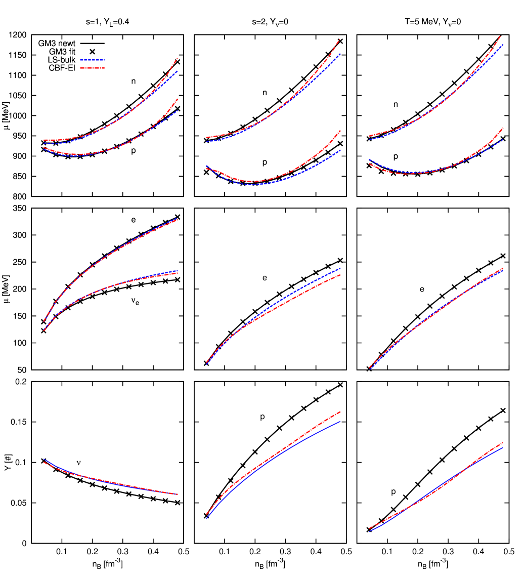
Figure 2.4: Comparison between the three EoSs used in this thesis, in the three regimes described in Sec. 2.8. In the top and middle rows, we plot the chemical potential (in regimes (ii) and (iii) $\mu_{\nu_{e}}=0$, because $Y_{\nu}=0$). In the lower row, we plot the particle abundances (the abundances not plotted may be easily determined with the relations $Y_{n}=1-Y_{p}$, $Y_{e}=Y_{p}$ and $Y_{L}=Y_{e}+Y_{\nu_{e}}$). The black solid line refers to the GM3 EoS determined by solving numerically the mean-field equations, the black crosses to the GM3 EoS determined through the fit and the procedure described in Sec. 2.7, the blue dashed line to the LS-bulk EoS, and the red dot-dashed line to the CBF-EI EoS.

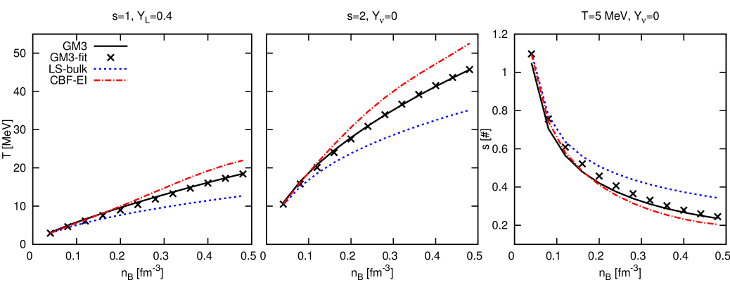
Figure 2.5: Comparison between the three EoSs in the three cases described in Sec. 2.8. In the left and central plots we show the temperature and in the right plot we show the entropy per baryon. Colors and line-styles are as in Fig. 2.4.

In Figs. 2.5 and 2.6 we show the dependence on the baryon number density of the temperature, entropy per baryon, pressure, energy density, and square of the sound speed,

$$c_{s}^{2}=\left.\frac{\partial P}{\partial\epsilon}\right|_{s,Y_{L}},$$ (2.141)

for the three EoSs in the three different regimes. The pressure and energy density in the three regimes have a very similar dependence on the number density, since their major contribute is due to the baryon interaction and degeneracy (Pons et al.,, 1999), rather than being thermal. At saturation density $n_{s}$ (whose exact value is slightly different for the three EoSs, but is in the range $n_{s}=0.15\textrm{-}0.16\,\mathrm{fm^{-3}}$), the sound speed is slightly larger (smaller) for the EoS with larger (smaller) imcompressibility parameter $K_{s}$. At high baryon density, the sound speed of the CBF-EI EoS is larger than that of the LS-bulk and GMr EoSs; this is due to a well-known problem of the many-body EoSs, which violate causality at very high density. However, in the regime of interest for this thesis, this unphysical behaviour can safely be neglected. We also notice that at given entropy per baryon $s$ and baryon density $n_{\mathrm{B}}$ the LS-bulk EoS is colder than GM3 EoS, whereas CBF-EI EoS is hotter than GM3 EoS (see Fig. 2.5). The LS-bulk EoS is colder because we do not include thermal contributions to the interacting part of the LS-bulk EoS, Eq. (2.66), and therefore the entropy is given only by the kinetic part. On the other hand, the CBF-EI EoS is hotter because the interaction is stronger for the CBF-EI, and therefore the (negative) entropy contribution is larger: the mean-field EoS is “more disordered” than the many-body one. In fact, the interaction lowers the total entropy, see Figs. 2.2 and 2.3, see also the right panel of Fig. 2.5. Therefore, fixing the total entropy contribution, the corresponding temperature is lower for the LS-bulk EoS, and higher for CBF-EI EoS.

In Fig 2.8 we plot the neutrino diffusion coefficient $D_{2}$, the electron neutrino scattering mean free path, and the baryon effective masses at different regimes — the incident neutrino energy used to compute the neutrino mean free path is $E_{\nu_{e}}=\max(\mu_{\nu_{e}},\pi T)$. To understand the role of interaction and finite temperature in the neutrino diffusion, we consider their effects on the baryon distribution function. To illustrate that, it is useful to look at the behaviour of the function

$$f_{a}(x)=\left(1+\mathrm{e}^{\frac{x}{a}}\right)^{-1}\rightarrow\frac{1}{h^{3}}\left(1+\mathrm{e}^{\frac{k^{2}}{2m^{\ast}T}-\frac{\mu-U-m}{T}}\right)^{-1},$$ (2.142)

where $a$ plays the role of the temperature $T$ and/or effective mass $m^{\ast}$, as it is clear after making a suitable change of variable that makes $f_{a}(x)$ the distribution function of a non-relativistic Fermion gas [right part of Eq. (2.142)]. As it is apparent from Fig. 2.7, $f_{a}$ approaches a theta-function as $a$ decreases, whereas increasing $a$ it becomes smoother.

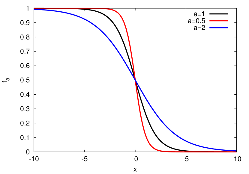
Figure 2.7: Plot of the “distribution function” of Eq. (2.142), varying the value of the parameter $a$.

Returning to the problem of neutrino diffusion, this means that for lower temperatures $T$ and effective masses $m^{\ast}$ (i.e., lower $a$), the baryon function becomes steeper, low-energy neutrinos can interact only with particles near the Fermi sphere, and therefore the mean free paths and diffusion coefficients increase. Conversely, a greater temperature and effective mass means that the particle distribution function is smoother, low-energy neutrinos may interact with more particles (since the Pauli blocking effect is lower), and therefore the mean free paths and the diffusion coefficients are smaller. The scattering mean free paths reflect the temperature dependence of the three EoSs: when the matter is hotter, the scattering is more effective (cf. Fig. 2.5 and the left and central plots of the middle row of Fig. 2.8). At equal temperature, the interaction is more effective when the effective mass is greater (right plot of the lower row of Fig. 2.8, cf. effective masses in Fig. 2.8). The behaviour of the diffusion coefficient $D_{2}$ (higher row of Fig. 2.8) results from a complex interplay between scattering and absorption, for which the effective masses and single particle potentials play an important role. The comparison between the diffusion coefficient $D_{2}$ for the three EoSs suggests that towards the end of the cooling phase (in which the thermodynamical conditions are roughly similar to the case (iii) described in this section), the CBF-EI star evolves faster than the other EoSs.

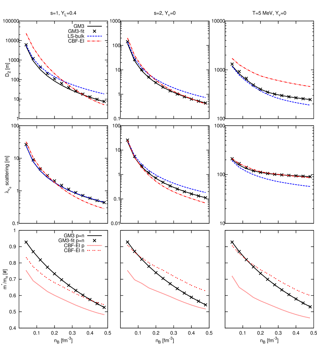
Figure 2.8: Comparison between the diffusion coefficient $D_{2}$ (upper panel), the electron neutrino scattering mean free paths [middle panel, the neutrino incoming energy is $E_{\nu_{e}}=\max(\mu_{\nu_{e}},\pi T)$], and the baryon effective masses, $m^{\ast}/m_{n}$ (lower panel) for the three EoSs considered in this thesis in the three cases described in Sec. 2.8. For the GM3 EoS, the effective masses of proton and neutron are identical Glendenning, (1985); Glendenning and Moszkowski, (1991). We do not show the LS-bulk EoS effective masses, since we have set them equal to the bare ones, $m^{\ast}_{\{p,n\}}/m_{n}=1$. Colors and line-styles are as in Fig. 2.4, apart for the line-styles in the lower panel, where the CBF-EI proton (neutron) effective masses are dotted (double-dashed).

Chapter 3 Proto-neutron star evolution

The evolution of the proto-neutron star phase, despite of being simpler to study with respect to the precedent core collapse and core bounce phases, has received a relatively smaller attention in the literature than the former phases. In fact, the main focus of numerical relativity groups has been to develop codes that could handle the more complex and shorter (up to hundreds of milliseconds) explosion phase. Nevertheless, there exist codes written for the PNS phase (Burrows and Lattimer,, 1986; Keil and Janka,, 1995; Pons et al.,, 1999; Roberts,, 2012). These codes have been used to study the evolutionary dynamics of the PNS (Burrows and Lattimer,, 1986), the neutrino detection from this phase (Burrows,, 1988; Keil and Janka,, 1995; Pons et al.,, 1999), the dependence of the evolution on the underlying EoS (Burrows,, 1988; Keil and Janka,, 1995; Pons et al.,, 1999; Roberts et al.,, 2012 but to our knowledge the case of a many-body EoS has never been studied), to presence of accretion (Burrows,, 1988), and to determine whether and under which conditions a black hole would form in a SN event (Burrows,, 1988; Keil and Janka,, 1995; Pons et al.,, 1999). Roberts, (2012) wrote a spectral PNS evolution code to study the nucleosynthesis due to neutrino interaction with the SN remnant (Roberts et al.,, 2012). Miralles et al., (2000) and Roberts et al., (2012) also studied the PNS evolution with convection.

The study of the gravitational waves from quasi-normal oscillations, emitted during the PNS phase, has been done only with the GM3 mean-field EoS by Ferrari et al., (2003). The case of a PNS with a many-body EoS (that of Burgio and Schulze,, 2010) has been studied by Burgio et al., (2011), where the authors mimic the PNS time evolution using some reasonable but not self-consistently evolved radial profiles of entropy per baryon and lepton fraction. The main goal of this thesis is to determine how the GW frequencies emitted during the PNS phase depends on the underlying EoS in a self-consistent fashion. Since the timescale of interest for the GW emission in the PNS phase is on the order of ten seconds (Ferrari et al.,, 2003; Burgio et al.,, 2011), we have to follow the evolution of the PNS during this period. We have therefore written a general (i.e., that could be run with a general EoS) evolutionary PNS code.

In this chapter we discuss the approximations, the equations, and the code used to follow the PNS evolution, and describe the results with the three different nuclear EoSs introduced in Chapter 2 and with three stellar baryon masses $M_{B}=1.25,1.40,1.60\mathrm{M_{\odot}}$. In Sec. 3.1 we discuss the equations of stellar structure, that is, the Tolman-Oppenheimer-Volkoff equations. Then we derive the neutrino transport equations that determine the time evolution of the PNS, first empirically in Sec. 3.2, and then rigorously in Sec. 3.3. In Sec. 3.4 we describe the numerical implementation of the PNS evolution that, even though simpler than the implementation of a SN explosion code, is not trivial at all. The last two sections, in which we describe the differences for the three EoSs and the three stellar masses in the PNS evolution (Sec. 3.5) and in the neutrino signal in a terrestrial detector (Sec. 3.6), contain the main original results of this chapter (Camelio et al.,, 2017).

3.1 Stellar structure equation (TOV)

Describing the evolution of a star means that one knows the stellar structure at each time. What we mean with “stellar structure” is the knowledge of the (radial, since we work in spherical symmetry) profiles of the local and integrated physical quantities. With “local” we refer to the thermodynamical quantities and to the metric functions (that are defined below), and with “integrated” we refer for example to the baryonic or gravitational mass enclosed in a radius $r$. Since, as we will show later, the evolution of a PNS is quasi-stationary, the stellar structure is given by the so called TOV equations, which determine the structure of a static and spherical star. In this section we discuss the TOV equations and recast them in a form which is more suitable to our case, that is, for a PNS.

To obtain the TOV equations, one first considers the most general static and spherically symmetric metric, that may be written as

$$\mathrm{d}s^{2}=-\mathrm{e}^{2\phi}\mathrm{d}t^{2}+\mathrm{e}^{2\lambda}\mathrm{d}r^{2}+r^{2}\mathrm{d}\theta^{2}+r^{2}\sin^{2}\theta\mathrm{d}\varphi^{2}.$$ (3.1)

where $\phi\equiv\phi(r)$ and $\lambda\equiv\lambda(r)$ are metric functions that depend only on the coordinate radius $r$, since we have imposed staticity and spherical symmetry. One then assumes that the matter may be described by a perfect fluid, that is, shear stresses and energy transport are negligible. Since we want to study the evolution of a PNS, the latter condition may seem contradictory. However, the quasi-stationarity of the PNS evolution guarantees that the energy transport is negligible on a hydrodynamic timescale, which is the timescale in which the star rearranges itself reaching structural equilibrium, and which is therefore the timescale relevant for the TOV equations. The perfect fluid stress-energy tensor is given by

$$T^{\mu\nu}=(\epsilon+P)u^{\mu}u^{\nu}+Pg^{\mu\nu},$$ (3.2)

where $\epsilon$ is the total (of all species, included the neutrinos) energy density, $P$ is the pressure, $g^{\mu\nu}$ is the metric, and $u^{\mu}$ the fluid four-velocity. Then, one usually considers the four equations of the energy-momentum conservation,

$$T^{\mu\nu}_{\hphantom{\mu\nu};\nu}=0,$$ (3.3)

plus $6$ other equations from the $16$ field equations

$$G_{\mu\nu}=8\pi GT_{\mu\nu},$$ (3.4)

where $G_{\mu\nu}$ is the Einstein field tensor. After the calculations (for details, see e.g. Misner et al.,, 1973, Chapter 23), one obtains inside the star

$$\frac{\mathrm{d}P}{\mathrm{d}r}=-\frac{(\epsilon+P)(m+4\pi r^{3}P)}{r(r-2m)},$$ (3.5)

where

$$m(r)=\int_{0}^{r}4\pi r^{2}\epsilon\mathrm{d}r,$$ (3.6)

is the total mass-energy inside radius $r$. Eqs. (3.5) and (3.6) are the TOV equations. The relation between $\epsilon$ and $P$ is given by the EoS. However, as we have seen in Chapter 2, the PNS EoS is not barotropic, that is, it depends on more than one variable, for example it depends also on the entropy per baryon $s$ and the lepton fraction $Y_{L}$, $\epsilon\equiv\epsilon(P,s,Y_{L})$. Therefore, to integrate the TOV equations, one needs information on the stellar thermal and composition content, that is, one needs to know the entropy and lepton fraction profiles, $s(r)$ and $Y_{L}(r)$.

The other quantities that determine the stellar structure are similarly obtained,

$$\frac{\mathrm{d}\phi}{\mathrm{d}r}={} \frac{m+4\pi r^{3}P}{r(r-2m)},$$ (3.7)

$$a(r)={} \int_{0}^{r}4\pi r^{2}n_{\mathrm{B}}\mathrm{e}^{\lambda}\mathrm{d}r,$$ (3.8)

$$\lambda(r)={} -\frac{1}{2}\log\big{(}1-2m(r)/r\big{)},$$ (3.9)

$$m_{\mathrm{B}}(r)={} m_{n}a(r),$$ (3.10)

where $a(r)$ and $m_{\mathrm{B}}(r)$ are the total baryon number and total baryon mass enclosed in a sphere of radius $r$.

It is easy to cast the stellar structure equations (3.5)-(3.8) in the following form,

$$\frac{\mathrm{d}r}{\mathrm{d}a}={} \frac{1}{4\pi r^{2}n_{\mathrm{B}}\mathrm{e}^{\lambda}},$$ (3.11)

$$\frac{\mathrm{d}m}{\mathrm{d}a}={} \frac{\epsilon}{n_{\mathrm{B}}\mathrm{e}^{\lambda}},$$ (3.12)

$$\frac{\mathrm{d}\phi}{\mathrm{d}a}={} \frac{\mathrm{e}^{\lambda}}{4\pi r^{4}n_{\mathrm{B}}}(m+4\pi r^{3}P),$$ (3.13)

$$\frac{\mathrm{d}P}{\mathrm{d}a}={} -(\epsilon+P)\frac{\mathrm{e}^{\lambda}}{4\pi r^{4}n_{\mathrm{B}}}(m+4\pi r^{3}P),$$ (3.14)

where $\lambda$ is given by Eq. (3.9). We have chosen as independent variable the enclosed baryon number $a$, that is a more natural independent variable than the radius $r$. In fact, as we have discussed in Chapter 2, all particles but neutrinos are locked during the timescale of PNS evolution, and therefore the total entropy $S$, lepton number $N_{L}$, and baryon number $N_{\mathrm{B}}$ contained in the $i$-th stellar layer (which is centered in $a_{i}$ and whose baryon content is $\mathrm{d}a_{i}$) is conserved during the evolution, apart for the entropy and lepton number moved from that layer to the neighbouring ones by neutrino diffusion (see Secs. 3.2 and 3.3). As before, to solve the TOV equations one needs information on the stellar thermal and composition content, and therefore needs the profiles $s(a)$ and $Y_{L}(a)$.

The structure equations (3.11)–(3.14) are completed by the boundary conditions

$$m(a=0)={} 0,$$ (3.15)

$$r(a=0)={} 0,$$ (3.16)

$$P(a=A)={} P_{s},$$ (3.17)

$$\phi(a=A)={} \frac{1}{2}\log(1-2M/R),$$ (3.18)

where $A$ is the PNS total baryon number (that is conserved during the evolution, since we do not account for accretion or expulsion of material from the PNS), $R=r(a=A)$ and $M=m(a=A)$ are the stellar radius and the total gravitational mass, respectively, and $P_{s}$ is the surface pressure, that is, a very low pressure that defines for numerical purposes the stellar border. The exact value of $P_{s}$ does not influence the determination of the stellar structure, provided that it is sufficiently low.

The numerical solution of the stellar structure equations (3.11)–(3.14) with the boundary conditions (3.15)–(3.18) is not trivial and is discussed in Sec. 3.4.

3.2 Neutrino transport equations: semi-empirical derivation

The PNS structure changes in its first minute of life because the EoS depends on the temperature and lepton fraction, which change due to the neutrino diffusion. The hydrodynamical timescale is shorter than the neutrino diffusion timescale, and hence one can describe the PNS evolution as a sequence of quasi-stationary configurations; then, the evolutionary timescale is determined by neutrinos. This means that, to determine the PNS evolution, one has first to describe the neutrino diffusion process, that is, to obtain the neutrino transport equations. In this section we present a pedagogical introduction to the transport equations, dropping all the complications related to GR. This should give a direct physical insight that is absent from the rigorous derivation of the neutrino transport equations, which is given in the next section.

A mathematical model for the diffusion of a salt in a liquid was proposed for the first time by Fick in 1855 (Fick,, 1855, see Fick,, 1995 for an English reprint of the original article), in analogy to the Fourier mathematical model for heat transport and Ohm theory for the diffusion of electricity in a conductor. Even though the original Fick laws are, strictly speaking, incorrect for the study of the PNS evolution, they have a more immediate physical interpretation; moreover, a naïve generalization of Fick laws has been used in the first codes of PNS evolution (Burrows and Lattimer,, 1986; Keil and Janka,, 1995). Here we obtain the Fick laws with a simple argument. We consider the diffusion of a particle species in 1D (e.g., a tube). Between the coordinates $x-\mathrm{d}x/2$ and $x+\mathrm{d}x/2$ (a cell centered in $x$) there are $N(x)$ particles of that species and between $x+\mathrm{d}x/2$ and $x+3/2\mathrm{d}x$ (a cell centered in $x+\mathrm{d}x$) there are $N(x+\mathrm{d}x)$. If $v$ is the speed of the particles along $x$, $\mathrm{d}t=\mathrm{d}x/v$ is the time that a particle employs to cross the distance $\mathrm{d}x$. If all particles have the same speed $v$, in a time $\mathrm{d}t$ half of the particles in the cell centered in $x+\mathrm{d}x$ move to the left (in $x$), and half of the particles in the cell centered in $x$ move to the right (in $x+\mathrm{d}x$). Then, the net number of particles that move from $x$ to $x+\mathrm{d}x$ are $-\frac{1}{2}N(x+\mathrm{d}x)+\frac{1}{2}N(x)$, and the corresponding net flux is

$$F=-\frac{1}{2}\left(\frac{N(x+\mathrm{d}x)}{A\mathrm{d}t}-\frac{N(x)}{A\mathrm{d}t}\right),$$ (3.19)

where $A$ is the section of the tube. Multiplying both the numerator and the denominator by $\mathrm{d}x^{2}$, and calling $n(x)=N(x)/A\mathrm{d}x$ the particle number density in $x$, we obtain the first Fick law,

$$F(x)={} -D\frac{\mathrm{d}n}{dx},$$ (3.20)

$$D={} \frac{\mathrm{d}x^{2}}{2\mathrm{d}t}=\frac{v\mathrm{d}x}{2},$$ (3.21)

where $D$ is called diffusion coefficient and it is related to the speed $v$ of the particles. In a time $\mathrm{d}t$, the number of particles in $x$ may change due to the incoming flux from $x-\mathrm{d}x$, the outgoing flux in $x+\mathrm{d}x$, and eventually due to particle generation in $x$,

$$N(x,t+\mathrm{d}t)-N(x,t)=A\mathrm{d}t\big{(}F(x-\mathrm{d}x/2)\\ -F(x+\mathrm{d}x/2)+S(x)n_{\mathrm{fluid}}\mathrm{d}x\big{)},$$ (3.22)

where $n_{\mathrm{fluid}}$ is the fluid particles number density and $S(x)$ is the number of particle created in $x$ per each fluid particle and per unit time $\mathrm{d}t$. The Fick second law is obtained by dividing the previous expression by $\mathrm{d}tA\mathrm{d}x$,

$$\frac{\partial n}{\partial t}+\frac{\partial F}{\partial x}\equiv\frac{\partial n}{\partial t}-D\frac{\partial^{2}n}{\partial x^{2}}=S(x)n_{\mathrm{fluid}},$$ (3.23)

where we have assumed that the diffusion coefficient $D$ is constant along the tube.

In three dimensions the second Fick law may be written as (Burrows and Lattimer,, 1986; Keil and Janka,, 1995, see e.g.. At variance with them, here we drop the GR terms to simplify the discussion)

$$\frac{\partial Y_{i}}{\partial t}+\frac{1}{4\pi r^{2}n_{\mathrm{B}}}\frac{\partial(4\pi r^{2}F_{i})}{\partial r}=\frac{\partial Y_{i}}{\partial t}+\frac{\partial(4\pi r^{2}F_{i})}{\partial a}=S_{i},$$ (3.24)

where $Y_{i}=n_{i}/n_{\mathrm{B}}$, $F_{i}$, and $S_{i}$ are the number fraction, the number flux, and the number source of the $i$-th particle, respectively, and $a$ is the enclose baryon number. We put the total baryon number $N_{\mathrm{B}}$ in the shell $\mathrm{d}a$ inside the time differentiation because the baryons are locked during the PNS evolution and the baryon number inside the shell $\mathrm{d}a$ is conserved. A rigorous justification of this step will be given in the next section.

Apart for the neutrino diffusion, there is neither particle nor heat flow through the stellar layers during the timescale of the PNS evolution. Therefore, the energy transport equation is

$$\frac{\partial e}{\partial t}+P\frac{\partial(1/n_{\mathrm{B}})}{\partial t}+\sum_{i}\frac{\partial(4\pi r^{2}H_{i})}{\partial a}=0,$$ (3.25)

where $e=E/N_{\mathrm{B}}$ is the total (of all kinds of particle) energy per baryon and $H_{i}$ is the energy flux due to particle $i$ (in our case, neutrino species $i$). To understand the equation, one should realize that the first two terms represent the change of the internal energy plus the work of compression $P\mathrm{d}V/\mathrm{d}t$. There is no energy source term as in the equation for the number transport because the energy gained (lost) by one particle is lost (gained) by the rest of the matter (there are no energy sinks), and hence the total sum is null: the total energy can vary only because of the net flux of energy $\sum_{i}H_{i}$ and by the work of compression.

The fluxes are proportional to the gradients of the number and energy density of the $i$-th particle and are usually written as (Burrows and Lattimer,, 1986; Keil and Janka,, 1995)

$$F_{i}={} -D_{i}^{n}\frac{\partial n_{i}}{\partial r},$$ (3.26)

$$H_{i}={} -D_{i}^{\epsilon}\frac{\partial\epsilon_{i}}{\partial r},$$ (3.27)

$$D_{i}^{n}={} \frac{c\lambda_{i}^{n}}{3},$$ (3.28)

$$D_{i}^{\epsilon}={} \frac{c\lambda_{i}^{\epsilon}}{3},$$ (3.29)

where $D_{i}^{n,\epsilon}$ are the diffusion coefficients of particle $i$, and $\lambda_{i}^{n}$ is the spectral average of the $i$-th particle mean free path, and $\lambda_{i}^{\epsilon}$ is the spectral average of the $i$-th particle mean free path equivalent to the Rosseland mean free path in the photon case (cf. Eqs. (3.26)–(3.29) with Eqs. (3.20)–(3.21) of this thesis; see also Eqs. (A6), (A11), and (A12) of Keil and Janka,, 1995).

Now we specialize Eqs. (3.24) and (3.25) to our case. We have set $\mu_{\nu_{\mu}}=\mu_{\bar{\nu}_{\mu}}=\mu_{\nu_{\tau}}=\mu_{\bar{\nu}_{\tau}}\equiv 0$, and therefore $Y_{L_{\mu}}=Y_{L_{\tau}}\equiv 0$: only the electron neutrino fraction $Y_{\nu_{e}}\equiv Y_{L}$ may change. Beta-equilibrium implies that $S_{\nu}=-S_{e}$, that is, for each electron neutrino that is created, an electron is destroyed, and viceversa. Finally, as we have already discussed, only neutrinos move through the stellar layers. Therefore, summing Eq. (3.24) for electrons to the same equation for neutrinos, one obtains

$$\frac{\partial Y_{L}}{\partial t}+\frac{\partial(4\pi r^{2}F_{\nu_{e}})}{\partial a}=0.$$ (3.30)

Finally, using Eqs. (2.11) and (2.43), one may rewrite Eq. (3.25) as

$$T\frac{\partial s}{\partial t}+\mu_{\nu_{e}}\frac{\partial Y_{L}}{\partial t}+\sum_{i\in\{e,\mu,\tau\}}\frac{\partial(4\pi r^{2}H_{\nu_{i}})}{\partial a}=0,$$ (3.31)

since also muon and tauon neutrinos move energy and entropy through the stellar layers (but not lepton number, see discussion above).

In the next section we consistently derive the transport equation in GR; however, it is instructive to empirically modify Eqs. (3.24) and (3.25) to include the effects of GR. This may be done by including a redshift term for the energies and temperatures, and including the time lapse effect in the derivatives with respect to the comoving frame, $\mathrm{d}\tau\rightarrow\mathrm{e}^{-\phi}\mathrm{d}\tau$. Then, the transport equations (3.30) and (3.31) becomes

$$\frac{\partial Y_{\mathrm{L}}}{\partial t}+\frac{\partial(4\pi r^{2}\mathrm{e}^{\phi}F_{\nu})}{\partial a}={} 0,$$ (3.32)

$$\mathrm{e}^{\phi}T\frac{\partial s}{\partial t}+\mathrm{e}^{\phi}\mu_{\nu}\frac{\partial Y_{\mathrm{L}}}{\partial t}+\frac{\partial(4\pi r^{2}\mathrm{e}^{2\phi}H_{\nu})}{\partial a}={} 0,$$ (3.33)

where there are no modification to the derivatives with respect to the time $t$ measured by an observer at infinity. Eqs. (3.32) and (3.33) close the stellar structure equations, which need the entropy and density profiles at each timestep to be solved. The numerical solution of the transport equations is discussed in Sec. 3.4.

3.3 Neutrino transport equations: rigorous derivation

In this section, following Pons et al., (1999), we give a rigorous derivation of the neutrino transport equations in GR, that have been obtained in a semi-empirical way in Sec. 3.2.

We take the static spherical metric of Eq. (3.1) and consider a frame comoving with the matter [with our assumptions, the four velocity of the matter is $\mathbf{u}=(\mathrm{e}^{-\phi},0,0,0)$]. The comoving basis $\{\mathbf{e}_{a}\}$ is defined by [Misner et al.,, 1973, Eq. (23.15a)]

$$\mathbf{e}_{a}\cdot\mathbf{e}_{b}={} \eta_{ab},$$ (3.34)

$$\mathbf{e}_{0}\equiv{} \mathbf{u}=\mathrm{e}^{-\phi}\partial_{t},$$ (3.35)

$$\mathbf{e}_{1}={} \mathrm{e}^{-\lambda}\partial_{r},$$ (3.36)

$$\mathbf{e}_{2}={} \frac{1}{r}\partial_{\theta},$$ (3.37)

$$\mathbf{e}_{3}={} \frac{1}{r\sin\theta}\partial_{\varphi},$$ (3.38)

and therefore the non-zero tetrad components are

$$e^{t}_{0}={} =(e^{0}_{t})^{-1}=\mathrm{e}^{-\phi},$$ (3.39)

$$e^{r}_{1}={} =(e^{1}_{r})^{-1}=\mathrm{e}^{-\lambda},$$ (3.40)

$$e^{\theta}_{2}={} =(e^{2}_{\theta})^{-1}=\frac{1}{r},$$ (3.41)

$$e^{\varphi}_{3}={} =(e^{3}_{\varphi})^{-1}=\frac{1}{r\sin\theta},$$ (3.42)

In an orthonormal basis [Misner et al.,, 1973, Eqs. (8.24b) and (8.14)],

$$[\mathbf{e}_{a},\mathbf{e}_{b}]={} (e_{a}^{\alpha}\partial_{\alpha}e_{b}^{\beta}-e_{b}^{\alpha}\partial_{\alpha}e_{a}^{\beta})\partial_{\beta}=c_{ab}^{\hphantom{ab}c}\mathbf{e}_{c},$$ (3.43)

$$c_{abc}={} \eta_{cd}c_{ab}^{\hphantom{ab}d},$$ (3.44)

$$\Gamma^{b}_{\hphantom{b}mn}={} \frac{\eta^{ba}}{2}(c_{amn}+c_{anm}-c_{mna}),$$ (3.45)

where the non-zero commutation coefficients $c_{abc}$ are

$$c_{010}={} -c_{100}=-\mathrm{e}^{-\lambda}\partial_{r}\phi,$$ (3.46)

$$c_{011}={} -c_{101}=-\mathrm{e}^{-\phi}\partial_{t}\lambda,$$ (3.47)

$$c_{122}={} -c_{212}=c_{133}=-c_{313}=-\frac{\mathrm{e}^{-\lambda}}{r},$$ (3.48)

$$c_{233}={} -c_{323}=-\frac{\cot\theta}{r},$$ (3.49)

and the non zero Ricci rotation coefficients are

$$\Gamma^{1}_{00}={} \Gamma^{0}_{10}=\mathrm{e}^{-\lambda}\partial_{r}\phi,$$ (3.50)

$$\Gamma^{0}_{11}={} \Gamma^{1}_{01}=\mathrm{e}^{-\phi}\partial_{t}\lambda,$$ (3.51)

$$\Gamma^{1}_{22}={} -\Gamma^{2}_{12}=\Gamma^{1}_{33}=-\Gamma^{3}_{13}=-\frac{\mathrm{e}^{-\lambda}}{r}$$ (3.52)

$$\Gamma^{2}_{33}={} -\Gamma^{3}_{23}=-\frac{\cot\theta}{r}.$$ (3.53)

The Boltzmann equations for massless particles in GR are [Lindquist,, 1966, Eq. (2.34)]

$$p^{b}\left(e_{b}^{\beta}\frac{\partial f}{\partial x^{\beta}}-\Gamma^{a}_{bc}p^{c}\frac{\partial f}{\partial p^{a}}\right)=\left(\frac{\mathrm{d}f}{\mathrm{d}\tau}\right)_{\mathrm{coll}},$$ (3.54)

where $f$ is the invariant neutrino distribution function, and $p^{a}$ is the neutrino four momentum in the comoving basis [cf. Lindquist,, 1966, Eq. (3.3)],

$$p^{a}=(E,E\mu,E\sqrt{1-\mu^{2}}\cos\bar{\varphi},E\sqrt{1-\mu^{2}}\sin\bar{\varphi}),$$ (3.55)

where $E$ is the neutrino energy, $\mu\equiv\cos\bar{\vartheta}$ is the cosine of the neutrino four momentum with respect to the radial direction, and $\bar{\varphi}$ is the angle of the neutrino four momentum with respect to the $\theta$ direction. Since in spherical symmetry $f\equiv f(t,r,E,\mu)$, we would express the derivatives with respect to $p^{a}$ as derivatives with respect to $E$ and $\mu$. We first notice that

$$E={} \sqrt{p_{1}^{2}+p_{2}^{2}+p_{3}^{2}}\equiv p_{0},$$ (3.56)

$$\mu={} \frac{p_{1}}{\sqrt{p_{1}^{2}+p_{2}^{2}+p_{3}^{2}}},$$ (3.57)

$$\frac{\partial f}{\partial p^{a}}\mathrm{d}p^{a}={} \frac{\partial f}{\partial E}\mathrm{d}E+\frac{\partial f}{\partial\mu}\mathrm{d}\mu,$$ (3.58)

$$\mathrm{d}E={} \alpha\{\mu\mathrm{d}p_{1}+\sqrt{1-\mu^{2}}\cos\bar{\varphi}\mathrm{d}p_{2}+\sqrt{1-\mu^{2}}\sin\bar{\varphi}\mathrm{d}p_{3}\}$$

$$+(1-\alpha)\mathrm{d}p_{0},$$ (3.59)

$$\mathrm{d}\mu={} \frac{1-\mu^{2}}{E}\mathrm{d}p_{1}-\frac{\mu\sqrt{1-\mu^{2}}\cos\bar{\varphi}}{E}\mathrm{d}p_{2}-\frac{\mu\sqrt{1-\mu^{2}}\sin\bar{\varphi}}{E}\mathrm{d}p_{3},$$ (3.60)

where $\alpha$ is an arbitrary parameter that we have included to stress the freedom we have in expanding the differential of $\mathrm{d}E$. This freedom is due to the reduced number of variables ($E$ and $\mu$ instead of $p^{a}$, $a=0\ldots 3$) on which the distribution function explicitly depends after the change of variable (the following calculations do not depend on the exact value of $\alpha$, and we shall set it equal to zero to simplicity). Then,

$$\frac{\partial f}{\partial p^{0}}={} (1-\alpha)\frac{\partial f}{\partial E},$$ (3.61)

$$\frac{\partial f}{\partial p^{1}}={} \alpha\mu\frac{\partial f}{\partial E}+\frac{1-\mu^{2}}{E}\frac{\partial f}{\partial\mu},$$ (3.62)

$$\frac{\partial f}{\partial p^{2}}={} \alpha\sqrt{1-\mu^{2}}\cos\bar{\varphi}\frac{\partial f}{\partial E}-\mu\frac{\sqrt{1-\mu^{2}}}{E}\cos\bar{\varphi}\frac{\partial f}{\partial\mu},$$ (3.63)

$$\frac{\partial f}{\partial p^{3}}={} \alpha\sqrt{1-\mu^{2}}\sin\bar{\varphi}\frac{\partial f}{\partial E}-\mu\frac{\sqrt{1-\mu^{2}}}{E}\sin\bar{\varphi}\frac{\partial f}{\partial\mu},$$ (3.64)

and, after lengthy but straightforward calculations, Eq. (3.54) becomes [cf. Lindquist,, 1966, Eq. (3.8a)]

$$\mathrm{e}^{-\phi}E\partial_{t}f+\mathrm{e}^{-\lambda}E\mu\partial_{r}f-E^{2}\left(\mu\mathrm{e}^{-\lambda}\partial_{r}\phi+\mu^{2}\mathrm{e}^{-\phi}\partial_{t}\lambda\right)\partial_{E}f\\ +E(1-\mu^{2})\left(\frac{\mathrm{e}^{-\lambda}}{r}-\mathrm{e}^{-\lambda}\partial_{r}\phi-\mu\mathrm{e}^{-\phi}\partial_{t}\lambda\right)\partial_{\mu}f=\left(\frac{\mathrm{d}f}{\mathrm{d}\tau}\right)_{\mathrm{coll}}.$$ (3.65)

We remark that in Eq. (3.65) the arbitrary parameter $\alpha$ has disappeared.

It is customary to work with the angular moments of Eq. (3.65) (Lindquist,, 1966; Thorne,, 1981). Since we are interested in the zeroth and first moment of the Boltzmann-Lindquist equation, we apply to Eq. (3.65) the operator

$$\frac{1}{2}\int_{-1}^{+1}\mu^{i}\mathrm{d}\mu^{i}\qquad i=\{0;1\},$$ (3.66)

obtaining two equations [cf. Pons et al.,, 1999, Eqs. (6)–(7)],

$$\mathrm{e}^{-\phi}E\partial_{t}M_{0}+\mathrm{e}^{-\lambda}E\partial_{r}M_{1}-E^{2}(\mathrm{e}^{-\lambda}\phi^{\prime}\partial_{E}M_{1}+\mathrm{e}^{-\phi}\dot{\lambda}\partial_{E}M_{2})\\ +E\mathrm{e}^{-\lambda}\left(\frac{1}{r}-\phi^{\prime}\right)2M_{1}+E\mathrm{e}^{-\phi}\dot{\lambda}(M_{0}-3M_{2})=Q_{0},$$ (3.67)

$$\mathrm{e}^{-\phi}E\partial_{t}M_{1}+\mathrm{e}^{-\lambda}E\partial_{r}M_{2}-E^{2}(\mathrm{e}^{-\lambda}\phi^{\prime}\partial_{E}M_{2}+\mathrm{e}^{-\phi}\dot{\lambda}\partial_{E}M_{3})\\ +E\mathrm{e}^{-\lambda}\left(\frac{1}{r}-\phi^{\prime}\right)(3M_{2}-M_{0})+2E\mathrm{e}^{-\phi}\dot{\lambda}(M_{1}-2M_{3})=Q_{1},$$ (3.68)

where $\phi^{\prime}=\partial_{r}\phi$, $\dot{\lambda}=\partial_{t}\lambda$, and

$$M_{i}={} \frac{1}{2}\int_{-1}^{+1}\mu^{i}f\mathrm{d}\mu,$$ (3.69)

$$Q_{i}={} \frac{1}{2}\int_{-1}^{+1}\mu^{i}\left(\frac{\mathrm{d}f}{\mathrm{d}\tau}\right)_{\mathrm{coll}}\mathrm{d}\mu,$$ (3.70)

are the moments of the distribution function and of the source term. Since we are interested in energy averaged equations, we apply to Eq. (3.67) the operators

$$4\pi\int_{0}^{\infty}\mathrm{d}EE,$$ (3.71)

$$4\pi\int_{0}^{\infty}\mathrm{d}EE^{2},$$ (3.72)

obtaining

$$\mathrm{e}^{-\phi}\partial_{t}n_{\nu}+\mathrm{e}^{-\lambda}\left(\partial_{r}F_{\nu}+\phi^{\prime}F_{\nu}+\frac{2}{r}F_{\nu}\right)+\mathrm{e}^{-\phi}\dot{\lambda}n_{\nu}={} S_{N},$$ (3.73)

$$\mathrm{e}^{-\phi}\partial_{t}\epsilon_{\nu}+\mathrm{e}^{-\lambda}\left(\partial_{r}H_{\nu}+2\phi^{\prime}H_{\nu}+\frac{2}{r}H_{\nu}\right)+\mathrm{e}^{-\phi}\dot{\lambda}(\epsilon_{\nu}+P_{\nu})={} S_{E},$$ (3.74)

where

$$n_{\nu}={} 4\pi\int_{0}^{\infty}\mathrm{d}EM_{0}E^{2},$$ (3.75)

$$F_{\nu}={} 4\pi\int_{0}^{\infty}\mathrm{d}EM_{1}E^{2},$$ (3.76)

$$S_{N}={} 4\pi\int_{0}^{\infty}\mathrm{d}EQ_{0}E,$$ (3.77)

$$\epsilon_{\nu}={} 4\pi\int_{0}^{\infty}\mathrm{d}EM_{0}E^{3},$$ (3.78)

$$H_{\nu}={} 4\pi\int_{0}^{\infty}\mathrm{d}EM_{1}E^{3},$$ (3.79)

$$P_{\nu}={} 4\pi\int_{0}^{\infty}\mathrm{d}EM_{2}E^{3},$$ (3.80)

$$S_{E}={} 4\pi\int_{0}^{\infty}\mathrm{d}EQ_{0}E^{2}.$$ (3.81)

Using the baryon number conservation equation in GR,

$$(nu^{a})_{;a}=\mathrm{e}^{-\phi}\partial_{t}n_{\mathrm{B}}+\mathrm{e}^{-\phi}\dot{\lambda}n_{\mathrm{B}}=0,$$ (3.82)

one obtains

$$\mathrm{e}^{-\phi}\left(\partial_{t}n_{\nu}-\frac{n_{\nu}}{n_{\mathrm{B}}}\partial_{t}n_{\mathrm{B}}\right)+\frac{\mathrm{e}^{-\lambda}\mathrm{e}^{-\phi}}{4\pi r^{2}}\partial_{r}(4\pi r^{2}\mathrm{e}^{\phi}F_{\nu})={} S_{N},$$ (3.83)

$$\mathrm{e}^{-\phi}\left(\partial_{t}\epsilon_{\nu}-\frac{\epsilon_{\nu}+P_{\nu}}{n_{\mathrm{B}}}\partial_{t}n_{\mathrm{B}}\right)+\frac{\mathrm{e}^{-\lambda}\mathrm{e}^{-2\phi}}{4\pi r^{2}}\partial_{r}(4\pi r^{2}\mathrm{e}^{2\phi}H_{\nu})={} S_{E},$$ (3.84)

and, multiplying Eqs. (3.83) and (3.84) by $\mathrm{e}^{\phi}/n_{\mathrm{B}}$, and using Eq. (3.11),

$$\partial_{t}Y_{\nu}+\partial_{a}(4\pi r^{2}\mathrm{e}^{\phi}F_{\nu})={} \mathrm{e}^{\phi}\frac{S_{N}}{n_{\mathrm{B}}},$$ (3.85)

$$\partial_{t}e_{\nu}-\frac{P_{\nu}}{n_{\mathrm{B}}^{2}}\partial_{t}n_{\mathrm{B}}+\mathrm{e}^{-\phi}\partial_{a}(4\pi r^{2}\mathrm{e}^{2\phi}H_{\nu})={} \mathrm{e}^{\phi}\frac{S_{E}}{n_{\mathrm{B}}},$$ (3.86)

where $Y_{\nu}=n_{\nu}/n_{\mathrm{B}}$ is the neutrino fraction and $e_{\nu}=\epsilon_{\nu}/n_{\mathrm{B}}$ the neutrino energy per baryon. As we have already discussed (Secs. 2.7 and 3.2), we assume that muon and tauon neutrinos have vanishing chemical potentials, and hence the only non vanishing neutrino number is the electron one, $Y_{\nu_{e}}$. Since we additionally assume beta-equilibrium, for each neutrino that is absorbed (emitted), there is an electron that is emitted (absorbed), and analogously for the antineutrinos/positrons. Moreover, electrons are locked in the timescales of PNS evolution, and therefore only neutrinos diffuse through the star. Then,

$$\partial_{t}Y_{e}=-\mathrm{e}^{\phi}\frac{S_{N}}{n_{\mathrm{B}}}.$$ (3.87)

Summing Eqs. (3.83) and (3.87), one finally obtains

$$\frac{\partial Y_{\mathrm{L}}}{\partial t}=-\frac{\partial(4\pi r^{2}\mathrm{e}^{\phi}F_{\nu})}{\partial a}.$$ (3.88)

Similarly, the energy gained (lost) by neutrinos is lost (gained) by the rest of the matter (in our case, protons, neutrons, electrons, and positrons),

$$\partial_{t}e_{\mathrm{matter}}-\frac{P_{\mathrm{matter}}}{n_{\mathrm{B}}^{2}}\partial_{t}n_{\mathrm{B}}=-\mathrm{e}^{\phi}\frac{S_{E}}{n_{\mathrm{B}}}.$$ (3.89)

Summing Eqs. (3.84) and (3.89), and using the thermodynamical relations (2.11) and (2.43), we finally obtain

$$T\frac{\partial s}{\partial t}+\mu_{\nu_{e}}\frac{\partial Y_{\mathrm{L}}}{\partial t}=-\sum_{i\in\{e;\mu;\tau\}}\mathrm{e}^{-\phi}\frac{\partial(4\pi r^{2}\mathrm{e}^{2\phi}H_{\nu_{i}})}{\partial a},$$ (3.90)

where $s$ is the total (matter plus neutrinos) entropy per baryon, and we have summed over all neutrino species because even though muon and tauon neutrinos have been assumed to have a (fixed and constant) vanishing chemical potential and then their respective lepton numbers are fixed and vanishing. In fact, they are not locked in the star and therefore can move energy through the stellar layers. We remark that Eqs. (3.88) and (3.90) are the same equations that we have previously obtained with a semi-empirical argument, Eqs. (3.32) and (3.33).

To obtain the relativistic expression for the neutrino number and energy fluxes, we have to make an assumption on the distribution function that allows to close the set of equations (3.67) and (3.68). This assumption is the so called diffusion approximation, that is, we expand the distribution function dependence on the angle made by the neutrino direction with the radial direction ($\bar{\vartheta}$, and $\mu\equiv\cos\bar{\vartheta}$) in Legendre polynomials and we retain only the first two moments,

$$f(E,\mu)=f_{0}(E)+\mu f_{1}(E),$$ (3.91)

where $f_{0}$ is the (ultra-relativistic) neutrino distribution function (see Appendix A). Then, the moments of the distribution function [Eq. (3.69)] become

$$M_{0}={} f_{0},$$ (3.92)

$$M_{1}={} \frac{1}{3}f_{1},$$ (3.93)

$$M_{2}={} \frac{1}{3}f_{0},$$ (3.94)

$$M_{3}={} \frac{1}{5}f_{1},$$ (3.95)

and the first moment of the Boltzmann-Lindquist equation [Eq. (3.68)] becomes (since the transport is driven by spatial gradients, we neglect time derivatives)

$$Q_{1}=\frac{E}{3}\mathrm{e}^{-\lambda}\left(\partial_{r}f_{0}-E\phi^{\prime}\partial_{E}f_{0}\right).$$ (3.96)

It is possible to show (Pons et al.,, 1999; Reddy et al.,, 1998) that

$$Q_{1}=-\frac{E}{3}f_{1}(E)\lambda_{\mathrm{tot}}^{-1}(E),$$ (3.97)

where $\lambda_{\mathrm{tot}}(E)$ is the total mean free path (due to scattering, absorption, emission, and their inverse processes, see Sec. 2.2) of a neutrino with energy $E$, and therefore

$$f_{1}=-\lambda_{\mathrm{tot}}(E)\mathrm{e}^{-\lambda}\left(\partial_{r}f_{0}-E\phi^{\prime}\partial_{E}f_{0}\right).$$ (3.98)

Since

$$\partial_{r}f_{0}={} +(2\pi\hbar)^{3}f_{0}(1-f_{0})\left(\partial_{r}\eta+\frac{E}{T^{2}}\partial_{r}T\right),$$ (3.99)

$$\partial_{E}f_{0}={} -(2\pi\hbar)^{3}f_{0}(1-f_{0})\frac{1}{T},$$ (3.100)

$$\eta\equiv{} \frac{\mu_{\nu_{e}}}{T},$$ (3.101)

from Eqs. (3.76), (3.79), (3.93), (3.98)–(3.101), we finally obtain (Pons et al.,, 1999)

$$F_{\nu_{i}}={} -\frac{\mathrm{e}^{-\lambda}\mathrm{e}^{-\phi}T^{2}}{6\pi^{2}\hbar^{3}}\Bigg{(}D_{3}^{i}\frac{\partial(T\mathrm{e}^{\phi})}{\partial r}+(T\mathrm{e}^{\phi})D_{2}^{i}\frac{\partial\eta}{\partial r}\Bigg{)},$$ (3.102)

$$H_{\nu_{i}}={} -\frac{\mathrm{e}^{-\lambda}\mathrm{e}^{-\phi}T^{3}}{6\pi^{2}\hbar^{3}}\Bigg{(}D_{4}^{i}\frac{\partial(T\mathrm{e}^{\phi})}{\partial r}+(T\mathrm{e}^{\phi})D_{3}^{i}\frac{\partial\eta}{\partial r}\Bigg{)},$$ (3.103)

$$D_{n}^{i}={} \int_{0}^{\infty}\mathrm{d}(E/T)(E/T)^{n}f^{i}_{0}(E)\big{(}1-f^{i}_{0}(E)\big{)}\lambda_{\mathrm{tot}}^{-1}(E),$$ (3.104)

where $F_{\nu}$ and $H_{\nu}$ are the neutrino number and energy fluxes, respectively, the index $i=\{e;\mu;\tau\}$ refers to the lepton family, $f_{0}^{i}$ is the Fermi-Dirac distribution function of the $i$-th neutrino at equilibrium and the integration is performed on the neutrino energy divided by the temperature, $E/T$. As already stated, only electron neutrinos move lepton number through the stellar layers, whereas all neutrinos move energy. This fact, together with the assumption of muon and tauon null chemical potential, permits to rewrite the transport equations in a simplified way (Pons et al.,, 1999),

$$F_{\nu}={} -\frac{\mathrm{e}^{-\lambda}\mathrm{e}^{-\phi}T^{2}}{6\pi^{2}\hbar^{3}}\Bigg{(}D_{3}\frac{\partial(T\mathrm{e}^{\phi})}{\partial r}+(T\mathrm{e}^{\phi})D_{2}\frac{\partial\eta}{\partial r}\Bigg{)},$$ (3.105)

$$H_{\nu}={} -\frac{\mathrm{e}^{-\lambda}\mathrm{e}^{-\phi}T^{3}}{6\pi^{2}\hbar^{3}}\Bigg{(}D_{4}\frac{\partial(T\mathrm{e}^{\phi})}{\partial r}+(T\mathrm{e}^{\phi})D_{3}\frac{\partial\eta}{\partial r}\Bigg{)},$$ (3.106)

$$\partial_{t}Y_{\mathrm{L}}+{} \frac{\partial 4\pi\mathrm{e}^{\phi}r^{2}F_{\nu}}{\partial a}=0,$$ (3.107)

$$T\partial_{t}s+{} \mu_{\nu_{e}}\partial_{t}Y_{\mathrm{L}}+\mathrm{e}^{-\phi}\frac{\partial 4\pi\mathrm{e}^{2\phi}r^{2}H_{\nu}}{\partial a}=0,$$ (3.108)

$$D_{2}={} D_{2}^{\nu_{e}}+D_{2}^{\bar{\nu}_{e}},$$ (3.109)

$$D_{3}={} D_{3}^{\nu_{e}}-D_{3}^{\bar{\nu}_{e}},$$ (3.110)

$$D_{4}={} D_{4}^{\nu_{e}}+D_{4}^{\bar{\nu}_{e}}+4D_{4}^{\nu_{\mu}},$$ (3.111)

where we have neglected the differences between muon and tauon neutrinos (and antineutrinos) in the microphysical processes.

Eqs. (3.105)–(3.111) have to be completed by boundary conditions. For the center of the star, these are the request of null fluxes, $F_{\nu}(r=0)=0$ and $H_{\nu}(r=0)=0$; for the stellar border, one has to do an assumption on the leaving neutrinos. Usually one assumes that the number and energy fluxes at the stellar border are proportional to the neutrino number and energy densities. The numerical solution of Eqs. (3.105)–(3.111) is discussed in the next section.

A final remark is in order. We notice that the “semi-empirical” definition of the fluxes (3.26)–(3.27) is equivalent (apart for the metric coefficients) to Eqs. (3.105)–(3.106), if we adopt for $n_{\nu}$ and $\epsilon_{\nu}$ the expressions (2.137) and (2.138), provided that the diffusion coefficients are

$$D_{2}\propto{} 3\eta^{2}+\pi^{2},$$ (3.112)

$$D_{3}\propto{} 3(\eta^{3}+\pi^{2}\eta),$$ (3.113)

$$D_{4}\propto{} 3\left(\eta^{4}+2\pi^{2}\eta^{2}+\frac{7}{5}\pi^{4}\right).$$ (3.114)

3.4 Numerical implementation

The equations that describe the PNS structure and evolution, Eqs. (3.11)–(3.14) and (3.105)–(3.108), are relatively simple. However, their numerical implementation is not trivial at all. In this section we discuss the subtleties involved.

The PNS has been evolved using a sequence of predictor-corrector steps, that is, one separately solves the structure and the transport equations, and then iterate to evolve the star. This method is equivalent to use a full implicit scheme (Pons et al.,, 1999). The iterative procedure is easier to understand by inspecting the skeleton of the code in top language,

# 1) iterating (predictor-corrector step) is equivalent
#    to solve the structure and transport equations
#    simultaneously
# 2) structure() solves the TOV equation (relaxation method)
# 3) transport() evolves the thermodynamical profiles
#    (implicit scheme)
main:
   load initial profiles (a, YL, s)
   (P, phi, r, m) = structure(YL, s, a)
   # evolve the star
   for each time:
      # iterate until convergence of YL’ and s’
      repeat:
         # determine the optimal timestep dt
         repeat:
            YL’’=YL’
            s’’=s’
            (YL’, s’) = transport(P, phi, r, m, YL, s, dt)
            temp = max(sum|s’-s’’|/sum|s’’|,
                       sum|YL’-YL’’|/sum|YL’’|)
            if(eps/2 < temp < eps*2):
               exit
            else:
               dt = dt * eps / temp
         (P, phi, r, m) = structure(YL’, s’, a)
         temp = max(sum|s’-s|/sum|s|, sum|YL’-YL|/sum|YL|)
         if(temp < tol):
            exit
      YL=YL’
      s=s’
      eventually, print the evolved profiles

Using the original stellar profiles $P(a)$, $m(a)$, $r(a)$ and $\phi(a)$, we have (i) first solved the transport equations, determining the evolved lepton fraction and entropy profiles, $s^{\prime}(a)$ and $Y_{L}^{\prime}(a)$. Then, (ii) using these evolved profiles, we have determined the new stellar structure, $P^{\prime}(a)$, $m^{\prime}(a)$, $r^{\prime}(a)$ and $\phi^{\prime}(a)$. Using these evolved stellar profiles, but the original lepton fraction and entropy profiles $s(a)$ and $Y_{L}(a)$, we have (ib) solved the transport equations obtaining the evolved $s^{\prime\prime}(a)$ and $Y_{L}^{\prime\prime}(a)$ profiles, from which we have obtained (iib) the evolved stellar profiles $P^{\prime\prime}(a)$, $m^{\prime\prime}(a)$, $r^{\prime\prime}(a)$ and $\phi^{\prime\prime}(a)$. We have iterated the steps (i)-(ii) until convergence of the evolved lepton fraction and entropy profiles.

In addition to the iteration between the structure and transport part (predictor-corrector step), we have also iterate to find the optimal timestep, that is, the timestep such that the maximum fractional change in the entropy and lepton fraction profiles is greater than eps/2 but smaller than 2*eps.

The usual procedure to solve the TOV equation is to fix the central pressure $P_{c}$ and then integrate Eq. (3.5) and (3.6) up to the final pressure $P_{s}$, whose exact value does not influence the determination of the stellar properties, provided that it is small enough. In this way, one obtains the total radius, gravitational mass, baryon mass, and the thermodynamical and metric profiles of a star with central pressure $P_{c}$. However, this procedure can not be applied to our case, since at each timestep one does not know the central pressure $P_{c}$ and conversely the total baryon mass of the PNS is fixed and constant during the evolution (since we do not include effects of accretion or mass ejection from the PNS), that is, one has to solve the structure equations with the boundary conditions (3.15)–(3.18). A simple way to achieve this is to use the shooting method, that is, one first solves the structure equations fixing a tentative central pressure $P^{\prime}_{c}$ and obtains a total baryon mass $M_{\mathrm{B}}^{\prime}$, then iteratively varies the central pressure until the right total baryon mass is reached within the given error. This method has the advantage to be conceptually simple, however (i) it is numerically quite slow (ii) it may fail to converge when it is used in combination with the Newton-Raphson procedure to determine the EoS. This is due to the fact that the intrinsic variability of the Newton-Raphson procedure does not allow to obtain an arbitrarily small accuracy in the mass determination. To circumvent this, one may (a) increase the precision of the Newton-Raphson procedure (but this lowers the chances of Newton-Raphson convergence), or (b) get the EoS quantities by table interpolation (but to get the EoS by table interpolation in a hydrodynamical code the second order derivatives must be continue, see Swesty,, 1996, and for an EoS with three independent variables this is quite complex, see discussion in Sec 2.6). We have therefore solved the structure equations with a relaxation method (see Press et al.,, 1992, Sec. 17.3), as done also in Pons et al., (1999). The relaxation method consists in iteratively modify a tentative solution of a given differential equation on a grid, until the differential equation is satisfied within a given error. To fix the ideas, we take a set of $N$ ordinary differential equations

$$\frac{\mathrm{d}\mathbf{y}}{\mathrm{d}x}=\mathbf{g}(x,\mathbf{y}),$$ (3.115)

where the $N$ functions $y_{i}$, with $i=1,\ldots,N$, are defined on a grid of $M$ points $x_{j}$, with $j=1,\ldots,M$ (we call $y_{i,j}$ the $j$-th point of the $i$-th function). If the differential equations are not fulfilled by the tentative solution $\mathbf{y}$, then

$$\mathbf{E}_{j}(\mathbf{y}_{j},\mathbf{y}_{j-1})=\mathbf{y}_{j}-\mathbf{y}_{j-1}-(x_{j}-x_{j-1})\frac{\mathbf{g}(x_{j},\mathbf{y}_{j})+\mathbf{g}(x_{j-1},\mathbf{y}_{j-1})}{2}\neq 0,$$ (3.116)

(Eq. (3.116) is valid for an internal point, $j=2,\ldots,M$, however it may be easily generalized for the boundary conditions, i.e. $j=1,M+1$) and the improved solution $\mathbf{y}^{\prime}$ of the differential equations $\mathbf{g}$,

$$\mathbf{y}^{\prime}=\mathbf{y}+\Delta\mathbf{y},$$ (3.117)

is given by the condition

$$\mathbf{E}_{j}(\mathbf{y}_{j}+\Delta\mathbf{y}_{j},\mathbf{y}_{j-1}+\Delta\mathbf{y}_{j-1})\simeq 0.$$ (3.118)

In other words, one must invert the system

$$\sum_{k=1}^{N}\frac{\partial E_{i,j}}{\partial y_{k,j}}\Delta y_{k,j}+\sum_{k=1}^{N}\frac{\partial E_{i,j-1}}{\partial y_{k,j-1}}\Delta y_{k,j-1}=-E_{i,j},$$ (3.119)

for $i=1,\ldots,N$ and $j=2,\ldots,M$ (plus the boundary conditions, $j=1,M+1$, that are similarly handled) to find $\Delta y_{i,j}$ and the improved solution $y^{\prime}_{i,j}$. This procedure is repeated until convergence (for details, see Press et al.,, 1992, Sec. 17.3). We have used the relaxation method to solve the set of structure equations (3.11)–(3.14), with the boundary conditions (3.15)–(3.18), on a grid of $124$ points. The EoS has been determined with a Newton-Raphson cycle.

The neutrino transport equations are diffusive equations, whose prototype is in the form (see Press et al.,, 1992, Secs. 19.1 and 19.2)

$$\frac{\partial y}{\partial t}-D\frac{\partial^{2}y}{\partial x^{2}}=0.$$ (3.120)

Numerically solving a diffusion equation, that is a parabolic equation, is not easy at all. The simpler numerical algorithm one can think of,

$$\frac{f^{t+\mathrm{d}t}_{i}-f^{t}_{i}}{\mathrm{d}t}={} D\frac{f^{t}_{i+1}-2f^{t}_{i}+f^{t}_{i-1}}{\mathrm{d}x^{2}},$$ (3.121)

$$f^{t+\mathrm{d}t}_{i}={} \left(\delta_{ij}+\frac{D\mathrm{d}t}{\mathrm{d}x^{2}}(\delta_{i+1,j}-2\delta_{i,j}+\delta_{i-1,j})\right)f^{t}_{j},$$ (3.122)

is called forward Euler and is not stable, unless one chooses a very low time-step $\mathrm{d}t$. Indeed, a stability analysis shows that the algorithm (3.121) is stable only if (Press et al.,, 1992, Sec. 19.2)

$$\frac{2D\mathrm{d}t}{\mathrm{d}x^{2}}\leq 1.$$ (3.123)

This condition can be understood with the following argument, called Courant condition. Eq. (3.121) implies that, from the point of view of the algorithm, the point $f_{i}^{t+\mathrm{d}t}$ depends only on the information present in the points $f_{i-1}^{t}$, $f_{i}^{t}$, and $f_{i+1}^{t}$. Since Eq. (3.120) determines the physical propagation velocity of the information [$v\simeq 2D/\mathrm{d}x$, cf. Eq. (3.21)], choosing a timestep too large one should also consider the information present in the other neighbouring points $f_{i+2}^{t}$, $f_{i-2}^{t}$, etc. Not doing that results in a numerical instability. In order to preserve causality, then, the timestep must be smaller than (the order of) the distance between two consecutive grid points times the dispersion velocity, Eq. (3.123). The forward Euler algorithm (3.121) is an explicit algorithm, because to obtain the value of the function at the next timestep $f^{t+\mathrm{d}t}$ one makes use of the values of the function at the previous timestep, $f^{t}$. Conversely, in an implicit algorithm the right hand of Eq. (3.120) is evaluated at the next timestep,

$$\frac{f^{t+\mathrm{d}t}_{i}-f^{t}_{i}}{\mathrm{d}t}={} D\frac{f^{t+\mathrm{d}t}_{i+1}-2f^{t+\mathrm{d}t}_{i}+f^{t+\mathrm{d}t}_{i-1}}{\mathrm{d}x^{2}},$$ (3.124)

$$f^{t}_{i}={} \left(\delta_{ij}-\frac{D\mathrm{d}t}{\mathrm{d}x^{2}}(\delta_{i+1,j}-2\delta_{i,j}+\delta_{i-1,j})\right)f^{t+\mathrm{d}t}_{j},$$ (3.125)

and the value of the function at the next timestep $f^{t+\mathrm{d}t}$ is determined by inverting Eq. (3.125). A stability analysis applied to the implicit algorithm shows that it is unconditionally stable, that is, it converges for whatever timestep $\mathrm{d}t$ one chooses. Of course, the smaller $\mathrm{d}t$, the more accurate the solution, that is, a numerical convergence does not imply a convergence to the true physical solution (Press et al.,, 1992, Sec. 19.2).

To specialize the implicit algorithm to our case, we notice that (i) on the right hand side $f\equiv(\mathrm{e}^{\phi}T,\eta)$, (ii) on the left hand side the time derivatives are performed to $Y_{L}\equiv Y_{L}(T,\eta)$ and $s\equiv s(T,\eta)$. Moreover, the diffusion coefficients are (iii) not constant and (iv) they depend on the EoS, $D_{i}\equiv D_{i}(T,\eta)$. It is easy to account for (i) and (ii), we just have to consider two equations instead of one and to consider the convenient thermodynamical derivatives. To handle (iii), we just determine the value of the diffusion coefficients on a staggered grid of $M-1$ points, whose knots $a_{i+1/2}$ are the enclosed baryon mass in a radius

$$r_{i+1/2}=\frac{r_{i+1}+r_{i}}{2},$$ (3.126)

see Press et al., (1992, Sec. 19.2). The conceptually more difficult difference between the neutrino diffusion Equations (3.88)–(3.90) and the idealized diffusion Equation (3.120) is encoded in (iv), that is, the diffusion coefficients depend on the value of $T$ and $\eta$, and therefore we should evaluate them at the next timestep, $D^{t+\mathrm{d}t}$. However, this would greatly increase the complexity of the numerical implementation; we therefore (as done also by Pons et al.,, 1999) do not include implicitly the dependence on the EoS in the diffusion coefficients, but evaluate them explicitly, that is, at the current timestep, $D^{t}$. The discretization of the neutrino transport equations (3.88)–(3.90) is

$$\left(\left.\frac{\partial(\mathrm{e}^{\phi}T)}{\partial Y_{L}}\right|_{j}^{t}\delta_{ij}-\tilde{D}^{YT}_{j+1/2}(\delta_{i+1,j}-\delta_{i,j})+\tilde{D}^{YT}_{j-1/2}(\delta_{i,j}-\delta_{i-1,j})\right)(\mathrm{e}^{\phi}T)^{t+\mathrm{d}t}_{j}\\ =\left.\frac{\partial(\mathrm{e}^{\phi}T)}{\partial Y_{L}}\right|_{i}^{t}(\mathrm{e}^{\phi}T)^{t}_{i},$$ (3.127)

$$\left(\left.\frac{\partial\eta}{\partial Y_{L}}\right|_{j}^{t}\delta_{ij}-\tilde{D}^{Y\eta}_{j+1/2}(\delta_{i+1,j}-\delta_{i,j})+\tilde{D}^{Y\eta}_{j-1/2}(\delta_{i,j}-\delta_{i-1,j})\right)\eta^{t+\mathrm{d}t}_{j}\\ =\left.\frac{\partial\eta}{\partial Y_{L}}\right|_{i}^{t}\eta^{t}_{i},$$ (3.128)

$$\left(\left[\frac{\partial(\mathrm{e}^{\phi}T)}{\partial Y_{L}}+\frac{\partial(\mathrm{e}^{\phi}T)}{\partial s}\right]_{j}^{t}\delta_{ij}-\tilde{D}^{sT}_{j+1/2}(\delta_{i+1,j}-\delta_{i,j})\right.\\ \left.+\tilde{D}^{sT}_{j-1/2}(\delta_{i,j}-\delta_{i-1,j})\right)(\mathrm{e}^{\phi}T)^{t+\mathrm{d}t}_{j}=\left[\frac{\partial(\mathrm{e}^{\phi}T)}{\partial Y_{L}}+\frac{\partial(\mathrm{e}^{\phi}T)}{\partial s}\right]^{t}_{i}(\mathrm{e}^{\phi}T)^{t}_{i},$$ (3.129)

$$\left(\left[\frac{\partial\eta}{\partial Y_{L}}+\frac{\partial\eta}{\partial s}\right]_{j}^{t}\delta_{ij}-\tilde{D}^{s\eta}_{j+1/2}(\delta_{i+1,j}-\delta_{i,j})\right.\\ \left.+\tilde{D}^{s\eta}_{j-1/2}(\delta_{i,j}-\delta_{i-1,j})\right)\eta^{t+\mathrm{d}t}_{j}=\left[\frac{\partial\eta}{\partial Y_{L}}+\frac{\partial\eta}{\partial s}\right]_{i}^{t}\eta^{t}_{i},$$ (3.130)

where $\tilde{D}^{YT}$, $\tilde{D}^{Y\eta}$, $\tilde{D}^{sT}$, and $\tilde{D}^{s\eta}$ are diffusion coefficients conveniently redefined to simplify the equations, explicitly (i.e., at the current time $t$) evaluated on the staggered grid. Eqs. (3.127)–(3.130) are valid for internal points of the grid. At the center of the star, we assume that the fluxes are null,

$$F_{\nu}(0)=0,$$ (3.131)

$$H_{\nu}(0)=0,$$ (3.132)

and at the border, that the fluxes are proportional to the neutrino number and energy densities,

$$F_{\nu}(A)=\alpha n_{\nu}(A),$$ (3.133)

$$H_{\nu}(A)=\alpha\epsilon_{\nu}(A),$$ (3.134)

where $A$ is the total baryon number of the star, $A\equiv a(R)$, and $\alpha\in(0,1)$ an arbitrary parameter. The diffusion approximation (Sec. 3.3) causes the fluxes computed via Eqs. (3.88) and (3.90) to exceed the black-body limit in regions of small optical depth (i.e., near the stellar border). To stabilize the code in this region, we apply the flux limiter $3\Lambda(x)$ of Levermore and Pomraning, (1981),

$$3\Lambda(x)={} \frac{3}{x}\left(\coth(x)-\frac{1}{x}\right),$$ (3.135)

$$F_{\nu}\rightarrow{} 3\Lambda(F_{\nu}/n_{\nu})F_{\nu},$$ (3.136)

$$H_{\nu}\rightarrow{} 3\Lambda(H_{\nu}/\epsilon_{\nu})H_{\nu}.$$ (3.137)

Our simulations start at $200\,\mathrm{ms}$ from the core bounce, when the evolution may be considered quasi-stationary. As Pons et al., (1999), our initial entropy and lepton fraction profiles are obtained from the core-collapse simulations of Wilson and Mayle, (1989), conveniently rescaled with the total PNS baryon mass, which has been fixed at the beginning of our simulations. We have done this since we expect that the masses in the inner core roughly contains a constant entropy and lepton fraction (Pons et al.,, 1999). The rescaling applied to the entropy and lepton fraction profiles is the following

$$s(a,t=200\,\mathrm{ms})={} \frac{M_{\mathrm{B}}}{M^{\prime}_{\mathrm{B}}}s^{\prime}\!\left(a^{\prime},t=200\,\mathrm{ms}\right),$$ (3.138)

$$Y_{L}(a,t=200\,\mathrm{ms})={} \frac{M_{\mathrm{B}}}{M^{\prime}_{\mathrm{B}}}Y_{L}^{\prime}\!\left(a^{\prime},t=200\,\mathrm{ms}\right),$$ (3.139)

$$a={} \frac{M_{\mathrm{B}}}{M^{\prime}_{\mathrm{B}}}a^{\prime},$$ (3.140)

where the prime refers to the reference profiles of Wilson and Mayle, (1989).

The code described in this section has been written from scratch in FORTRAN90, with some auxiliary FORTRAN77 subroutine from Press et al., (1992) and some other auxiliary subroutines provided by J. A. Pons.

3.5 Results: PNS evolution

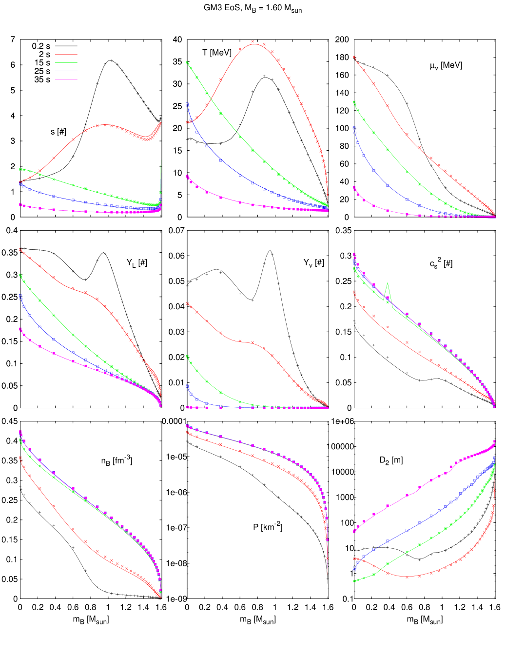
Figure 3.4: Stellar profiles at different times of the PNS evolved with the GM3 EoS. The solid lines correspond to the GM3 EoS determined with the methods explained in Sec. 2.4, the dots to the GM3 EoS determined by fitting the interacting contribution, see Secs. 2.6 and 2.7. From left to right and from top to bottom, we plot: the entropy per baryon, the temperature, the neutrino chemical potential, the lepton and neutrino fraction, the square of the speed of sound, the baryon density, the pressure and the diffusion coefficient $D_{2}$.

In this section we discuss the EoS and mass dependence of the evolution of a PNS. The EoSs we consider are those introduced in Chapter 2. In Table 3.1 we summarize the timescale of the evolution and the maximum central temperature for the three EoSs and three total baryon masses $M_{\mathrm{B}}=(1.25;1.40;1.60)\,\mathrm{M_{\odot}}$. In Figs. 3.1–3.3 we show the evolution of the central and maximum temperature, central entropy per baryon, central neutrino and proton fraction, and central baryon density for the same cases of Table 3.1. In Figs. 3.4–3.6 we show some snapshots of the stellar profiles (as a function of the enclosed baryon mass $m_{\mathrm{B}}$) of the entropy per baryon, temperature, neutrino chemical potential, lepton fraction, neutrino fraction, sound speed, baryon number density, pressure, and diffusion coefficient $D_{2}$ for the three EoSs, for a star with total baryonic mass $M_{\mathrm{B}}=1.60\,\mathrm{M_{\odot}}$. The times of the snapshots have been chosen to approximately describe the same periods of the stellar evolution; in fact the timescale of the evolution is different for each case considered.

As is shown in Figs. 3.1–3.3, the qualitative behaviour of the stellar evolution is the same for the three EoSs and the three stellar masses, even though the timescales and the thermodynamical profiles are quantitatively different. At the beginning of the evolution, which is 200 ms from core bounce, the PNS has a (relatively) low entropy core and a high entropy envelope. The neutrino chemical potential initially is very high in the center of the star; the process of neutrino diffusion transfers this degeneracy energy from neutrinos to the matter and this causes the heating of the PNS core. Moreover, on timescales of about 10 s, the star contracts from about $30$ km to its final radius of about $12$–$13$ km. The region which is affected the most from this contraction is the envelope, and in fact the contraction causes a consistent heating of the PNS envelope. At the same time, the steep negative neutrino chemical potential in the envelope causes a deleptonization of the envelope. The neutrinos leave the star, bringing with them energy. The joint effect of the envelope heating caused by contraction and cooling caused by neutrino emission is apparent in the behaviour of the maximum stellar temperature: before the central temperature reaches its maximum, the maximum stellar temperature increases, reaches a maximum value, and then decreases. During the progress of the evolution, the maximum stellar temperature position moves inward, until reaches the center of the star. Since the neutrino diffusion causes an heating of the PNS core (because as already explained the neutrino degeneracy energy is converted in thermal energy), it is not surprising that after some seconds the maximum stellar temperature increases again. This initial phase, during which the central temperature increases, lasts for several seconds and has been referred to as Joule heating phase in previous works. We may place the end of this phase at the end of the central temperature increase, that corresponds with the time at which the maximum temperature position reaches the center of the star. After the end of the Joule heating, there is a general cooling of the star as the deleptonization proceeds. Burrows and Lattimer, (1986) and Keil and Janka, (1995) found that the end of the Joule-heating phase coincides with the end of deleptonization, whereas Pons et al., (1999), with the GM3 EoS and with a more sensible treatment of the neutrino opacities, found that the deleptonization is longer than the Joule-heating phase. As Pons et al., (1999) we find that the deleptonization precedes the end of cooling for all the cases considered, however in the case of the CBF-EI we find that the most of neutrinos have been radiated by the end of the Joule-heating phase, that is, by the time at which the central temperature reaches its maximum value (Figs. 3.1–3.3, see Table 3.1).

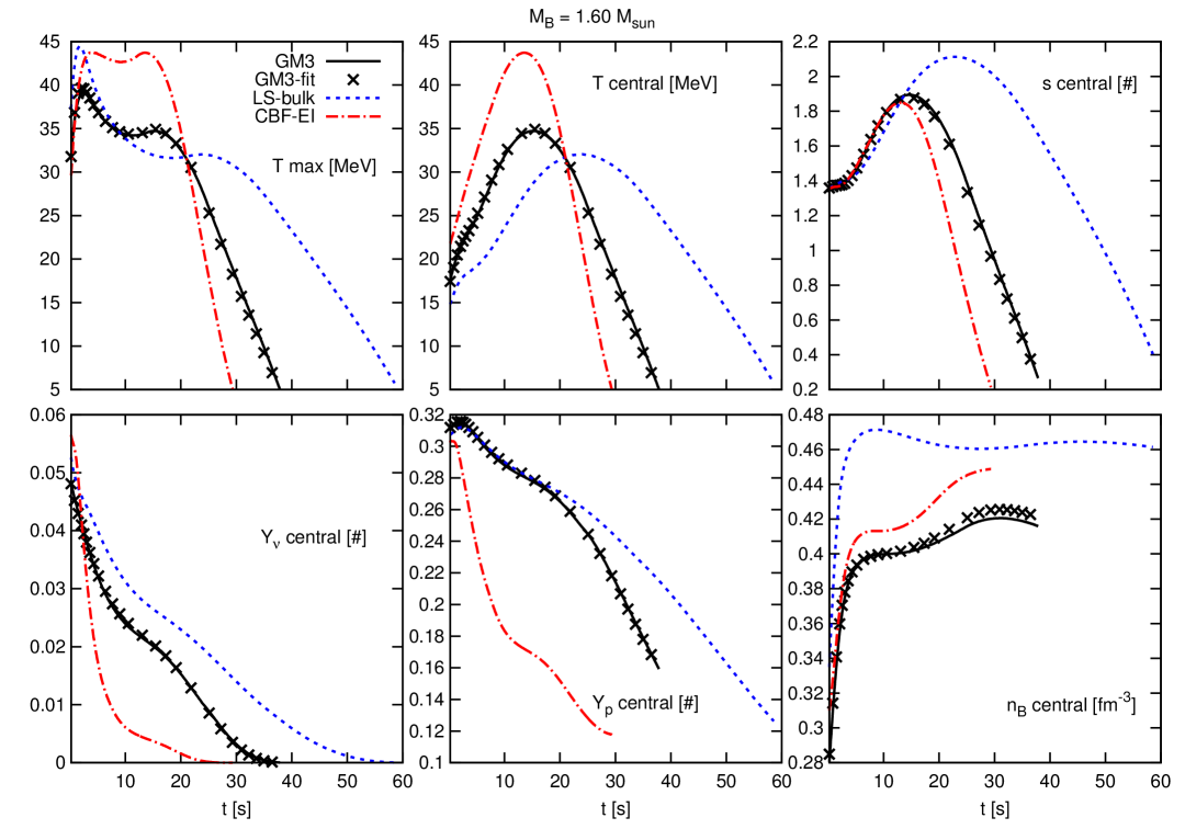
Figure 3.3: As in Fig 3.1, but for a star with $M_{\mathrm{B}}=1.60\,\mathrm{M_{\odot}}$.

Our results for the $M_{\mathrm{B}}=1.60\,\mathrm{M_{\odot}}$ PNS with the GM3 EoS are in qualitative agreement with those of Pons et al., (1999). In particular, the duration of the Joule-heating phase is in good agreement (cf. Fig. 3.3 of this thesis with Fig. 17 in Pons et al.,, 1999); however we find lower stellar temperatures and a shorter cooling phase than that found in Pons et al., (1999). We think that the quantitative differences between our results and those of Pons et al., (1999) are due to some differences in the initial profiles and in the details of the treatment of the diffusion process.

The PNS radius approaches its limiting value before the end of the cooling phase, while the gravitational mass has not completely reached its limiting value at the end of our simulation. This is due to the fact that we end our simulations when the central temperature is still relatively high, $T_{c}=5\,\mathrm{MeV}$. However, at this point the remnant energy to be emitted is small, and in fact the final luminosity is at least two orders of magnitude smaller than its initial value. We notice that the total gravitational mass at the end of the evolution is quite similar for the three EoSs. This is due to the fact that all considered EoSs are nucleonic EoSs, and therefore have a similar stiffness and stellar concentration (i.e., $M/R$), that largely determines the gravitational binding energy (and then the total gravitational mass). However, the gravitational mass for the three EoSs is not exactly the same, and this results in a different total neutrino emission, see Sec. 3.6.

For each EoS, the evolutionary timescales are smaller for a smaller stellar baryon mass. This is due to the way we have rescaled the initial entropy per baryon and lepton fraction profiles with the total stellar baryon mass, but also to the fact that a lower stellar mass is equivalent to lower densities and then to longer neutrino mean free paths. We also notice that a lower stellar mass corresponds to lower temperatures. This again depends on the initial entropy profiles and on the different densities present in the star, see Fig. 2.5: for a given entropy per baryon and lepton (or neutrino) fraction, lower densities correspond to lower temperatures. To overcome the uncertainties related to the initial configuration, in future we should use as initial profiles the ending configuration of core-collapse simulation of a star with the correct baryonic mass (see Pons et al.,, 1999 for a study on how the initial conditions affect the PNS evolution).

The fact that the LS-bulk evolution is slower than the GM3 one, which in turn is slower than that of the CBF-EI EoS, may well be explained by the fact that in the many-body CBF-EI EoS nuclear correlations are stronger than in the mean-field GM3 EoS, in which in turn are stronger than in the LS-bulk EoS (where the baryon masses are equal to the bare ones). A smaller neutrino cross section is a consequence of a greater baryon correlation (Sec. 2.8). This effect is relevant even at the mean-field level, where one adopts the description of the baryon spectra in term of effective masses and single-particle potentials to obtain the diffusion coefficients. For example, the fact that the proton effective mass is significantly smaller than the neutron one in the CBF-EI framework (Fig. 2.8) is a consequence of the tensor correlations which are stronger in the n-p channel than in the n-n or p-p channels.

To check this interpretation, that is, that the different timescales are mainly due to the details of the microphysics (i.e., the baryon spectra and hence the neutrino mean free paths and diffusion coefficients), we have run a simulation of a $M_{\mathrm{B}}=1.60\,\mathrm{M_{\odot}}$ PNS with the LS-bulk and CBF-EI EoSs, but with the diffusion coefficients of the GM3 EoS. As expected, we find out that the LS-bulk timescale is reduced with respect to that of a self-consistent simulation (i.e., using the LS-bulk diffusion coefficients), and the CBF-EI timescale is increased with respect to that of a self-consistent simulation. Of course, the timescales and the evolutionary profiles found in this non-consistent manner are not equal to those corresponding to the GM3 EoS, the differences due to the details of the EoS. For example, each EoS has a different thermal content and neutrino degeneracy, and different thermodynamical derivatives that determine how the stellar profiles change while energy and leptons diffuse through the star. Both the EoS and the neutrino mean free paths are important in determining the PNS evolution.

Table 3.1: Significant quantities describing the PNS evolution for the three EoSs described in this thesis and for three stellar baryon masses. The first column contains the name of the EoS, the second column contains the stellar baryon mass, the third and fourth columns contain the maximum central temperature and the corresponding time (the latter approximately corresponds to the end of the Joule-heating phase), respectively, the fifth column contains the time at which the central neutrino fraction becomes equal to $Y_{\nu}=0.005$ (this is an indication on the duration of the deleptonization phase), and the sixth column contains the time at which our simulation ends (namely, when the central temperature becomes equal to $T=5\,\mathrm{MeV}$). All simulations start at $t_{\mathrm{start}}=0.2\,\mathrm{s}$.

EOS	$M_{\mathrm{B}}$ [$M_{\odot}$]	$T_{\mathrm{max}}$ [MeV]	$t_{\mathrm{Jh}}$ [s]	$t_{\mathrm{del}}$ [s]	$t_{\mathrm{end}}$ [s]
GM3	1.25	24.6	9.0	13.1	20.8
GM3	1.40	28.7	11.2	18.6	27.1
GM3	1.60	34.9	15.2	27.9	37.7
LS-bulk	1.25	23.6	13.5	17.5	30.6
LS-bulk	1.40	26.6	17.6	26.3	41.0
LS-bulk	1.60	32.1	23.8	41.4	59.2
CBF-EI	1.25	32.3	7.31	3.46	17.0
CBF-EI	1.40	37.0	9.55	5.65	21.6
CBF-EI	1.60	43.7	13.6	11.7	29.4

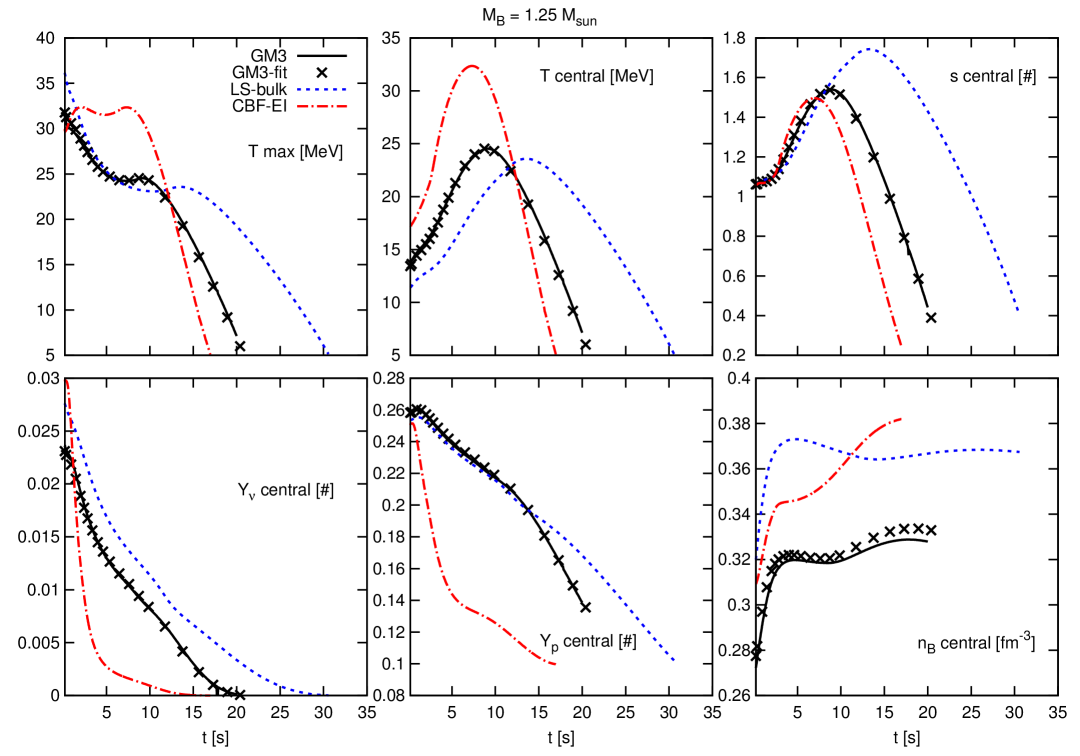
Figure 3.1: Time dependence of the maximum and central temperature (left and central upper plots), central entropy per baryon (right upper plot), neutrino and proton fraction (left and central lower plots) and central baryon density (right lower plot), for a star with total baryon mass $M_{\mathrm{B}}=1.25\,\mathrm{M_{\odot}}$ evolved using the three EoSs. Colors and line-styles are as in Fig. 2.4.

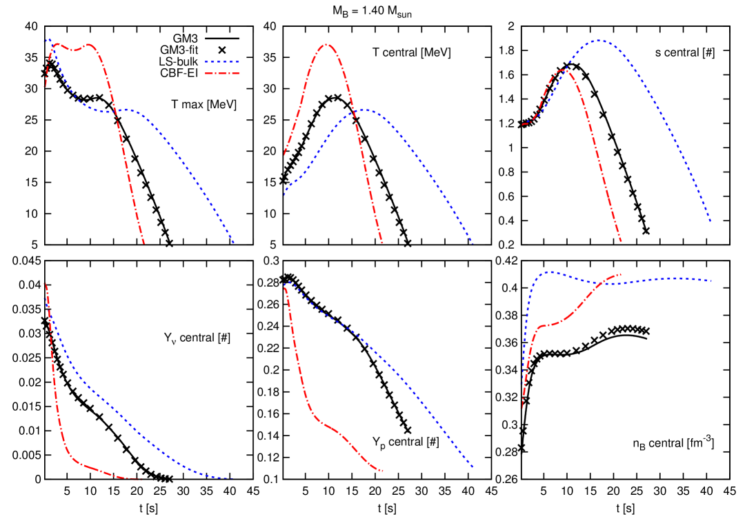
Figure 3.2: As in Fig 3.1, but for a star with $M_{\mathrm{B}}=1.40\,\mathrm{M_{\odot}}$.

Figure 3.5: As in Fig. 3.4, for the LS-bulk EoS.

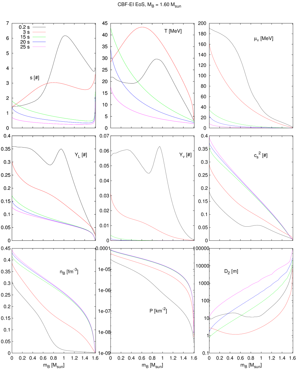
Figure 3.6: As in Fig. 3.4, for the CBF-EI EoS.

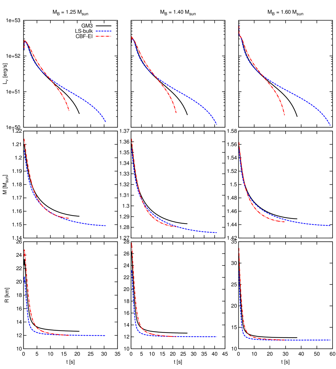
Figure 3.7: Time dependence of the total neutrino luminosity (upper panels), gravitational mass (middle panels), and stellar radius (lower panels) of a PNS evolved with the three EoSs considered in this thesis and the baryon stellar masses $M_{\mathrm{B}}=(1.25,1.40,1.60)\,\mathrm{M_{\odot}}$. Colors and line-styles as in Fig. 2.4. The gravitational masses at the end of the simulations are: for $M_{\mathrm{B}}=1.25M_{\odot}$, $M_{\mathrm{GM3}}=1.1554M_{\odot}$, $M_{\mathrm{LS-bulk}}=1.1492M_{\odot}$, $M_{\mathrm{CBF-EI}}=1.1548M_{\odot}$; for $M_{\mathrm{B}}=1.40M_{\odot}$, $M_{\mathrm{GM3}}=1.2824M_{\odot}$, $M_{\mathrm{LS-bulk}}=1.2750M_{\odot}$, $M_{\mathrm{CBF-EI}}=1.2806M_{\odot}$; and for $M_{\mathrm{B}}=1.60M_{\odot}$, $M_{\mathrm{GM3}}=1.4478M_{\odot}$, $M_{\mathrm{LS-bulk}}=1.4386M_{\odot}$, $M_{\mathrm{CBF-EI}}=1.4442M_{\odot}$.

3.6 Results: neutrino signal in terrestrial detectors

In 1987 a supernova (SN1987a) has been observed in the Large Magellanic Cloud (Kunkel et al.,, 1987). Together with the electromagnetic signal, 19 neutrinos were detected by the Cherenkov detectors Kamiokande II (Hirata et al.,, 1987) and IMB (Bionta et al.,, 1987), and 5 neutrinos at the Baksan underground scintillation telescope (Alekseev et al.,, 1987). These neutrinos have been observed on a timescales of ten seconds, and are therefore thought to have been emitted during the PNS phase. However, they were too few to accurately constrain the emitted neutrino spectrum and its time dependence (see e.g. Lattimer and Yahil,, 1989) and to give unambiguous answers about the proto-neutron star physics (Burrows,, 1988; Lattimer and Yahil,, 1989; Keil and Janka,, 1995; Pons et al.,, 1999). Today, with the current detectors, a SN event such that of the 1987 would generate $\sim 10^{4}$ neutrino detection (Ikeda et al.,, 2007), that would permit to accurately discriminate between the different physical scenarios that could occur during the PNS evolution. It is therefore fundamental to determine how the underlying EoS modifies the observed PNS neutrino signal. In this section we consider in particular the Super-Kamiokande III detector (Hosaka et al.,, 2006; Ikeda et al.,, 2007).

Our code has some limitations in reconstructing the emitted spectrum: we assume (i) beta-equilibrium, (ii) a Fermi distribution for all neutrino species, and (iii) a vanishing chemical potential for the muon and tauon neutrinos everywhere in the star. Assumptions (i) and (ii) are reasonable in the interior of the star, and lose accuracy near the stellar border, where the diffusion approximation breaks down and in practice the fluxes are always flux-limited (see Appendix B.2). To obtain a precise description of the neutrino emitted spectrum, one has to employ multi-flavour multi-group evolutionary codes (e.g., Roberts,, 2012), that also account for neutrino leakage near the stellar border. This is outside the aims of our work; however our approximations are reasonable as far as one is interested in total quantities, in particular the total neutrino luminosity $L_{\nu}$, which is equal to minus the gravitational mass variation rate,

$$L_{\nu}=\mathrm{e}^{2\phi}4\pi R^{2}H_{\nu}(R)=-\frac{\mathrm{d}M}{\mathrm{d}t},$$ (3.141)

where $H_{\nu}(R)$ is the neutrino energy luminosity at the stellar border (Figs. 3.1–3.3, lower-left plot).

We determine the formula to estimate the signal in terrestrial detectors following the discussion in Burrows, (1988) and applying a slight modification introduced by Pons et al., (1999), and we specify our results for the Super-Kamiokande III detector (Hosaka et al.,, 2006; Ikeda et al.,, 2007). The main reaction that occurs in a water detector like Super-Kamiokande is the electron antineutrino absorption on protons, $\bar{\nu}_{e}+p\rightarrow n+e^{+}$ [Ikeda et al.,, 2007, Eq. (1)], whose cross section for an antineutrino of energy $E$ is [Burrows,, 1988, Eq. (3c)]

$$\sigma_{p}\simeq{} \tilde{\sigma}_{0}(E-\Delta_{m})\sqrt{(E-\Delta_{m})^{2}-m_{e}^{2}},$$ (3.142)

$$\tilde{\sigma}_{0}={} 0.941\times 10^{-43}\,\mathrm{cm^{2}MeV^{-2}},$$ (3.143)

where we have neglected weak-magnetism corrections, $\Delta_{m}$ is the neutron-proton mass difference, and $m_{e}$ is the electron mass. We remark that since $\tilde{\sigma}_{0}$ has not the dimensions of a cross section (there is an additional factor $\mathrm{MeV^{-2}}$), we have explicitly put a tilde over it.

For each incoming neutrino, the detection probability is given by

$$P_{\bar{\nu}_{e}}=N_{p}\frac{4\pi\int_{E_{\mathrm{th}}}^{\infty}E^{2}f(E,\mathrm{e}^{\phi_{\nu}}T_{\nu},\mathrm{e}^{\phi_{\nu}}\mu_{\bar{\nu}_{e}})\sigma_{p}(E)W(E)\mathrm{d}E}{4\pi\int_{0}^{\infty}E^{2}f(E,\mathrm{e}^{\phi_{\nu}}T_{\nu},\mathrm{e}^{\phi_{\nu}}\mu_{\nu_{e}})\mathrm{d}E},$$ (3.144)

where $E_{\mathrm{th}}$ is the incoming neutrino energy threshold (to cut off the low-energy neutrino background that is a noise for high-energy SN and PNS neutrinos, Ikeda et al.,, 2007), $N_{p}$ is the number of free protons in the detector (i.e., the hydrogen atoms), $f$ is the electron antineutrino distribution function at the neutrinosphere, and $W(E)$ is the efficiency of the detector at incoming neutrino energy $E$. $\mathrm{e}^{\phi_{\nu}}$, $T_{\nu}$, and $\mu_{\bar{\nu}_{e}}$ are the redshift, temperature, and antineutrino chemical potential at the neutrinosphere, that is the sphere inside the PNS at whose radius $R_{\nu}$ neutrinos decouple from matter (therefore, $\mathrm{e}^{\phi_{\nu}}T_{\nu}$ and $\mathrm{e}^{\phi_{\nu}}\mu_{\bar{\nu}_{e}}$ are the temperature and the chemical potential at the neutrinosphere, seen by an observer at infinity), and the denominator is the antineutrino number density $n_{\bar{\nu}_{e}}$ at the neutrinosphere. The number flux of antineutrinos reaching the detector is given by

$$\frac{\mathrm{d}N_{\bar{\nu}_{e}}}{\mathrm{d}t}=\frac{4\pi R^{2}\mathrm{e}^{\phi}F_{\bar{\nu}_{e}}}{4\pi D^{2}},$$ (3.145)

where $D$ is the distance of the detector from the PNS and $4\pi R^{2}\mathrm{e}^{\phi}F_{\bar{\nu}_{e}}$ is the total (integrated over the sphere) number flux of electron antineutrinos at a radius $R\geq R_{\nu}$, seen by an observer at infinity. Our code determines better the total energy luminosity than the total number flux of antineutrinos and than the neutrinosphere radius (see discussion above), and therefore we make the replacements (at variance with Burrows,, 1988, and together with Pons et al.,, 1999) $4\pi R^{2}\mathrm{e}^{\phi(R)}F_{\bar{\nu}_{e}}\rightarrow L_{\bar{\nu}_{e}}$ and $n_{\bar{\nu}_{e}}\rightarrow\epsilon_{\bar{\nu}_{e}}$, where $L_{\bar{\nu}}$ is the total luminosity of the electron antineutrino and $\epsilon_{\bar{\nu}_{e}}$ its energy density (this latter computed at the neutrinosphere, see footnote 6). Putting together Eqs. (3.142), (3.144), and (3.145), and assuming a vanishing electron antineutrino chemical potential $\mu_{\bar{\nu}_{e}}=0$, we obtain

$$\frac{\mathrm{d}\mathcal{N}}{\mathrm{d}t}={} \frac{\tilde{\sigma}_{0}\tilde{n}_{p}\mathcal{M}}{4\pi D^{2}}\mathrm{e}^{\phi_{\nu}}T_{\nu}L_{\bar{\nu}_{e}}\frac{G_{W}(\mathrm{e}^{\phi_{\nu}}T_{\nu},E_{\mathrm{th}})}{6\operatorname{F_{3}}(0)},$$ (3.146)

$$6\operatorname{F_{3}}(0)={} \int_{0}^{\infty}\frac{x^{3}}{1+\mathrm{e}^{x}}\mathrm{d}x=\frac{7\pi^{4}}{120},$$ (3.147)

$$G_{W}(T,E_{\mathrm{th}})={} \int_{E_{\mathrm{th}}/T}^{\infty}\frac{x^{2}\left(x-\frac{\Delta}{T}\right)\sqrt{\left(x-\frac{\Delta}{T}\right)^{2}-\left(\frac{m_{e}}{T}\right)^{2}}}{1+\mathrm{e}^{x}}W(xT)\mathrm{d}x,$$ (3.148)

where $\tilde{n}_{p}\simeq 6.7\times 10^{31}\,\mathrm{kton^{-1}}$ is the number of free protons (i.e., hydrogen atoms) per unit water mass of the detector (this is the reason we put a tilde over it, since it is not defined in the same way we have defined a “number density” up to now), $\mathcal{M}$ is the water mass of the detector ($N_{p}=\mathcal{M}\tilde{n}_{p}$), $F_{3}$ is an ordinary Fermi integral and $G_{W}$ is a modified and truncated Fermi integral.

We take Super-Kamiokande III as reference detector, and therefore $\mathcal{M}\simeq 22.5\,\mathrm{ktons}$ (Ikeda et al.,, 2007), $E_{\mathrm{th}}=7.5\,\mathrm{MeV}$, and $W$ is reported in Hosaka et al., (2006, Fig. 3) and is unity for $E>E_{\mathrm{th}}$. We consider a galactic PNS, $D\simeq 10\,\mathrm{kpc}$, and assume the neutrinosphere to be at the radius at which the (total, of all flavours) neutrino energy flux becomes one third of the (total, of all flavours) neutrino energy density, $H_{\nu}/\epsilon_{\nu}=1/3$. Finally, we take the electron antineutrino energy to be one sixth of the total, $L_{\bar{\nu}_{e}}=L_{\nu}/6$, since (i) at the neutrinosphere all neutrino type chemical potentials are very small and therefore their energy density is very similar [the temperature term dominates, see Eq. (2.138)] and (ii) we do not account for neutrino oscillations (which should enhance the flux by about $10\%$, Ikeda et al.,, 2007).

The neutrino signal rate and total signal for the three EoSs are shown in Fig. 3.8. Since the binding energy of the cold neutron star of the three EoSs we consider is very similar (see Figs. 3.1–3.3), the total energy emitted by neutrinos during the PNS evolution is very similar too. On the other hand, the rate of antineutrino emission and the temperature at the neutrinosphere varies according to the underlying EoS. Therefore, there is an EoS signature on the cumulative antineutrino detection, and in particular for the CBF-EI, whose signal is noticeably larger than the other EoSs, even though its gravitational binding energy at the end of the evolution is between those of the LS-bulk and GM3 EoSs, see Figs. 3.1–3.3. This is due to the fact that the higher temperatures of the CBF-EI EoS cause a smoother antineutrino distribution function at the neutrinosphere, and hence more antineutrinos have an energy greater than the threshold $E_{\mathrm{th}}$ at the detector.

The different evolutionary timescales for the different EoSs and stellar masses correspond to different signal timescales, that may be easily inferred from the antineutrino detection rate. The antineutrino detection rates are qualitatively very similar between the three EoSs and the three stellar masses. During the first ten seconds the LS-bulk and GM3 stars have very similar detection rates and then diverge, the LS-bulk star having a longer evolution than the GM3 star. The CBF-EI star, instead, has the peculiarity of maintaining a higher antineutrino emission rate during the Joule-heating phase (approximately, during the first ten seconds), which is due to the faster deleptonization that we have already described in Sec. 3.5.

Figure 3.8: Signal in the Super-Kamiokande III Cherenkov detector, for the three EoSs considered in this thesis. On the top row, electron antineutrino detection rate; on the bottom row, electron antineutrino cumulative detection. On the left column, we consider a star with $M_{\mathrm{B}}=1.25\,\mathrm{M_{\odot}}$, on the central column $M_{\mathrm{B}}=1.40\,\mathrm{M_{\odot}}$, and on the right column $M_{\mathrm{B}}=1.60\,\mathrm{M_{\odot}}$.

To summarize, the analysis of the antineutrino detection rate and cumulative detection allows to determine the timescale of the evolution and to discriminate between the underlying EoS and the total stellar baryon mass. As a final remark, we point out again that, for a given mass, the total antineutrino detected do not depend uniquely on to the gravitational binding energy: for example the CBF-EI has a higher total antineutrino detection than the LS-bulk EoS, but a lower gravitational binding energy.

Chapter 4 Gravitational waves from stellar perturbation theory

The detection of the first gravitational wave signal (Abbot et al.,, 2016), emitted by two merging black holes, has hopefully started the era of “gravitational wave astronomy”, that promises to open a new observational window on our universe. The detection of a GW signal from a SN event would permit to explore the explosion process and the PNS formation, allowing to constrain the PNS physics. However, this would need an extended numerical study of the possible gravitational waveforms. Ferrari et al., (2003) have studied, using stellar perturbation theory, the gravitational emission during the first tens of seconds of the PNS life, evolved consistently with the mean-field GM3 EoS, also allowing for a hadron-quark transition in the core. Later, Burgio et al., (2011) have determined the quasi-normal modes frequencies of a PNS modeled with the many-body EoS of Burgio and Schulze, (2010), mimicking the PNS evolution with some reasonable thermal and composition profiles. Also Sotani and Takiwaki, (2016) have studied the gravitational wave emission (from proto-neutron stars with LS and Shen EoSs) using ad-hoc thermal profiles that mimic the evolution. To our knowledge, there are no studies of the GW emission from a PNS consistently evolved with a many-body EoS. Our aim is therefore to fill this gap, also providing a study of the dependence of the oscillation modes on the underlying EoS and stellar baryon mass.

In Chapter 3 we have discussed the PNS evolution with some different high-temperature EoSs, fixing different values of the total PNS baryon mass. In this chapter, we apply the relativistic theory of stellar perturbation to determine the frequencies at which a non-rotating PNS oscillates and emits gravitational waves, according to its underlying physics. In Sec. 4.1 we show how to find the frequencies of the quasi-normal modes and discuss their classification; in Sec. 4.2 we describe the code we have used to determine the stellar oscillations and compare the GW emitted signal for different EoSs and PNS masses. The results discussed in Sec. 4.2 are an original contribution of this thesis, and are also presented in Camelio et al., (2017).

4.1 Quasi-normal modes of a relativistic star

The Newtonian theory of stellar perturbations (e.g. Cox and Giuli,, 1968, Chapter 27) has been generalized to relativistic stars by Thorne and Campolattaro, (1967), and subsequently by Chandrasekhar and Ferrari, (1990). Using this theory one can determine the frequencies at which the star oscillates, radiating gravitational waves. These damped oscillations are the so-called quasi-normal modes of the star. In this section we briefly summarize the theory of stellar perturbation and of the quasi-normal modes and refer the interested reader to the cited literature for the details.

First of all, one makes the customary separation of the metric of the oscillating star $g_{\mu\nu}$ in a static and spherically symmetric background part $g_{\mu\nu}^{0}$ (obtained solving the TOV equations) and a perturbative part $h_{\mu\nu}$ which is a function of all coordinates,

$$g_{\mu\nu}(t,r,\theta,\varphi)=g^{0}_{\mu\nu}(r,\theta)+h_{\mu\nu}(t,r,\theta,\varphi),\qquad\mbox{with }|h_{\mu\nu}|\ll|g^{0}_{\mu\nu}|.$$ (4.1)

Since the star is perturbed, a fluid element that would be placed at $x^{\mu}$ in the equilibrium configuration moves to $x^{\mu}+\xi^{\mu}(x^{\nu})$, being $\xi^{\mu}$ the fluid displacement. At this point it is useful to introduce the concepts of Eulerian and Lagrangian perturbations of a particular quantity. To fix the ideas, we consider the pressure $P$, but it is trivial to generalize the discussion to other quantities, like the energy density or the baryon number density. An Eulerian perturbation of the pressure $\delta P$ at a point $x^{\mu}$ is defined by the variation of the pressure at $x^{\mu}$,

$$\delta P(x^{\mu})=P(x^{\mu})-P^{0}(x^{\mu}),$$ (4.2)

where $P$ and $P^{0}$ are the pressure of the perturbed and unperturbed star, respectively. The Lagrangian perturbation of the pressure $\Delta P$ at a point $x^{\mu}$ is defined as the variation of the pressure of the displaced fluid element that in the unperturbed star was in $x^{\mu}$, that is,

$$\Delta P(x^{\mu})=P(x^{\mu}+\xi^{\mu})-P^{0}(x^{\mu}).$$ (4.3)

In other words, the Lagrangian perturbation is the variation seen by an observer comoving with the perturbation. It is easy to convert an Eulerian perturbation into a Lagrangian one,

$$\Delta P(x^{\mu})\simeq\delta P(x^{\mu})+\frac{\partial P^{0}(x^{\mu})}{\partial x^{\nu}}\xi^{\nu}(x^{\mu}).$$ (4.4)

Choosing a suitable frame for which $\xi^{0}=0$, the stellar perturbation is defined by the unknown functions $\xi^{i}(x^{\alpha})$ ($i=\{1;2;3\}$) and $h_{\mu\nu}(x^{\alpha})$. The crucial point of the stellar perturbation theory is that the displacement vector $\xi^{i}$ and the metric perturbation tensor $h_{\mu\nu}$ are expanded in vector and tensor spherical harmonics, respectively. These were introduced by Regge and Wheeler, (1957), and we will follow their convention. Each harmonic basis element is determined by two indexes, that we customary call $l=0,\ldots,\infty$ (“the total angular momentum”) and $m$ (“the $z$ component of the angular momentum”, not to be confused with the enclosed gravitational mass). Since our background metric is spherically symmetric (i.e., the star is non rotating), there is degeneracy in the $m$ index, and then the resulting equations for two different values of $m$ are equivalent. To simplify the discussion, and without loss of generality, we will assume $m=0$. The index $l$ permits to classify the behaviour of the spherical harmonics under the parity operation, $\mathbf{r}\rightarrow-\mathbf{r}$. A harmonic that transforms as $(-1)^{l}$ under parity is called “even” (or “polar”, or “electric”), whereas if it transforms as $(-1)^{l+1}$ is called “odd” (or “axial”, or “magnetic”). Scalar harmonics are even, vector and tensor harmonics may be either even or odd. Making a suitable choice of the gauge, one can put to zero four components of the metric perturbation tensor $h_{\mu\nu}$. Many different choices of gauge are possible, and we will use the Regge-Wheeler gauge (Regge and Wheeler,, 1957).

Since the fluid is perturbed, the stress-energy tensor is perturbed too and one has to solve the perturbed Einstein equations and the perturbed continuity equations,

$$\delta G_{\mu\nu}={} 8\pi\delta T_{\mu\nu},$$ (4.5)

$$\delta(T_{\hphantom{\mu\nu};\nu}^{\mu\nu})={} 0,$$ (4.6)

where $G_{\mu\nu}$ is the Einstein tensor, $T_{\mu\nu}$ is the stress-energy tensor of the fluid composing the star, and $\delta$ is the Eulerian perturbation. At this point, one could Fourier-transform the equations and solve the perturbed equations for assigned values of the frequency $\omega$. We shall look for complex frequency solutions, i.e.

$$\omega=2\pi\nu+\frac{\imath}{\tau},$$ (4.7)

where $\nu$ is the (real) frequency of the perturbation and $\tau$ is the damping time. If the imaginary part of the complex frequency is zero, we would have normal modes, that is, stellar oscillation modes with amplitude constant in time (they do not grow nor damp). This is what happens in the Newtonian case, if one neglects viscosity forces. However, in GR, the imaginary part of the complex frequency is not zero due to gravitational wave emission, and therefore the stellar modes are called quasi-normal modes (QNMs).

Since the background metric is spherically symmetric, the perturbation equations for different angular momentum $l$ and different parity are decoupled. In particular, there are two distinct sets of equations, one for the even components and one for the odd ones. This allows a further simplification. The fluid quantities, that is, the pressure $P$, the energy density $\epsilon$, and the baryon density $n_{\mathrm{B}}$, are scalar quantities, and therefore do not appear in the odd-parity equations, since scalar harmonics are even. Purely gravitational modes, the so called w modes, are obtained from the odd equations, but since we are mainly interested in how the matter influences the gravitational wave emission, we shall not consider odd perturbations.

By expanding $h_{\mu\nu}$ in tensor spherical harmonics it is possible to show that the perturbed metric can be written as (Thorne and Campolattaro,, 1967; Detweiler and Lindblom,, 1985)

$$\mathrm{d}s^{2}=-\mathrm{e}^{2\phi}(1+r^{l}H_{0}Y_{lm}\mathrm{e}^{\imath\omega t+\imath m\varphi})\mathrm{d}t^{2}-2\imath\omega r^{l+1}H_{1}Y_{lm}\mathrm{e}^{\imath\omega t+\imath m\varphi}\mathrm{d}t\mathrm{d}r\\ +\mathrm{e}^{2\lambda}(1-r^{l}H_{0}Y_{lm}\mathrm{e}^{\imath\omega t+\imath m\varphi})\mathrm{d}r^{2}+r^{2}(1-r^{l}KY_{lm}\mathrm{e}^{\imath\omega t+\imath m\varphi})\mathrm{d}\Omega,$$ (4.8)

and the displacement vector as

$$\xi^{r}={} r^{l-1}\mathrm{e}^{-\lambda}W(r,\omega)Y_{lm}(\theta,\varphi)\mathrm{e}^{\imath\omega t+\imath m\varphi},$$ (4.9)

$$\xi^{\theta}={} -r^{l-2}V(r,\omega)\partial_{\theta}Y_{lm}(\theta,\varphi)\mathrm{e}^{\imath\omega t+\imath m\varphi},$$ (4.10)

$$\xi^{\varphi}={} -\frac{r^{l-2}{V(r,\omega)}}{\sin^{2}\theta}\partial_{\varphi}Y_{lm}(\theta,\varphi)\mathrm{e}^{\imath\omega t+\imath m\varphi},$$ (4.11)

where $Y_{lm}$ is the scalar spherical harmonic corresponding to indexes $l$ and $m$, and the functions $H_{0}$, $H_{1}$, $K$, $W$, $V$ depend on the radial coordinate $r$ and on the frequency $\omega$. They are the solution of a coupled set of equations obtained by inserting the metric (4.8) into Eqs. (4.5) and (4.6); setting the index $m=0$ these equations are ($m(r)$ is the gravitational mass)

$$\left(3m(r)+\frac{(l+2)(l-1)}{2}r+4\pi r^{3}P\right)H_{0}=8\pi r^{3}\mathrm{e}^{-\phi}X\\ +\left(\frac{1}{2}(l+2)(l-1)r-\omega^{2}r^{3}\mathrm{e}^{-2\phi}-\frac{\mathrm{e}^{2\lambda}}{r}\big{(}m(r)+4\pi r^{3}P\big{)}\big{(}3m(r)-r+4\pi r^{3}P\big{)}\right)K\\ -\left(\frac{l(l+1)}{2}\big{(}m(r)+4\pi r^{3}P\big{)}-\omega^{2}r^{3}\mathrm{e}^{-2(\phi+\lambda)}\right)H_{1},$$ (4.12)

$$X={} \omega^{2}(\epsilon+P)\mathrm{e}^{-\phi}V-\frac{\mathrm{e}^{\phi-\lambda}}{r}\frac{\mathrm{d}P}{\mathrm{d}r}W+\frac{\epsilon+P}{2}\mathrm{e}^{\phi}H_{0},$$ (4.13)

$$\frac{\mathrm{d}H_{1}}{\mathrm{d}r}={} -\left(l+1+\frac{2m(r)}{r}\mathrm{e}^{2\lambda}+4\pi r^{2}\mathrm{e}^{2\lambda}(P-\epsilon)\right)\frac{H_{1}}{r}$$

$$+\frac{\mathrm{e}^{2\lambda}}{r}\Big{(}H_{0}+K-16\pi(\epsilon+P)V\Big{)},$$ (4.14)

$$\frac{\mathrm{d}K}{\mathrm{d}r}={} \frac{H_{0}}{r}+\frac{l(l+1)}{2r}H_{1}-\left(\frac{l+1}{r}-\frac{\mathrm{d}\phi}{\mathrm{d}r}\right)K-8\pi\frac{\epsilon+P}{r}\mathrm{e}^{\lambda}W,$$ (4.15)

$$\frac{\mathrm{d}W}{\mathrm{d}r}={} -\frac{l+1}{r}W+r\mathrm{e}^{\lambda}\left(\frac{\mathrm{e}^{-\phi}}{(\epsilon+P)c_{s}^{2}}X-\frac{l(l+1)}{r^{2}}V+\frac{H_{0}}{2}+K\right),$$ (4.16)

$$\frac{\mathrm{d}X}{\mathrm{d}r}={} -\frac{l}{r}X+(\epsilon+P)\mathrm{e}^{\phi}\left\{\left(\frac{1}{r}-\frac{\mathrm{d}\phi}{\mathrm{d}r}\right)\frac{H_{0}}{2}\right.$$

$$+\left(r\omega^{2}\mathrm{e}^{-2\phi}+\frac{l(l+1)}{2r}\right)\frac{H_{1}}{2}+\left(3\frac{\mathrm{d}\phi}{\mathrm{d}r}-\frac{1}{r}\right)\frac{K}{2}-\frac{l(l+1)}{r^{2}}\frac{\mathrm{d}\phi}{\mathrm{d}r}V$$

$$\left.-\frac{1}{r}\left[4\pi(\epsilon+P)\mathrm{e}^{\lambda}+\omega^{2}\mathrm{e}^{\lambda-2\phi}-r^{2}\frac{\mathrm{d}}{\mathrm{d}r}\left(\frac{\mathrm{e}^{-\lambda}}{r^{2}}\frac{\mathrm{d}\phi}{\mathrm{d}r}\right)\right]W\right\},$$ (4.17)

where $\phi(r)$, $\lambda(r)$ [the metric functions defined in Eq. (3.1)], $m(r)$, $P(r)$, and $\epsilon(r)$ are the unperturbed quantities determined solving the TOV equations, the $c_{s}^{2}$ is the square of the speed of sound,

$$c_{s}^{2}=\left.\frac{\partial P}{\partial\epsilon}\right|_{s,Y_{L}},$$ (4.18)

and the auxiliary function $X(r,\omega)$ is proportional to the Lagrangian perturbation of the pressure,

$$\Delta P=-r^{l}\mathrm{e}^{-\phi}X(r).$$ (4.19)

To summarize, Eqs. (4.12)–(4.17) allow to determine the stellar perturbation in the interior of the star, for a fixed harmonic angular momentum $l$ and for a complex pulsation $\omega$. Since these equations are singular at $r=0$, to obtain physical solutions (i.e., regular at $r=0$), one has to expand the functions near the center, obtaining

$$H_{1}(r)={} H_{1}(0)+O(r^{2}),$$ (4.20)

$$K(r)={} K(0)+O(r^{2}),$$ (4.21)

$$W(r)={} W(0)+O(r^{2}),$$ (4.22)

$$X(r)={} X(0)+O(r^{2}),$$ (4.23)

$$H_{1}(0)={} \frac{2lK(0)+16\pi(\epsilon_{c}+P_{c})W(0)}{l(l+1)},$$ (4.24)

$$X(0)={} (\epsilon_{c}+P_{c})\mathrm{e}^{\phi}\left(\left(\frac{4\pi}{3}(\epsilon_{c}+3P_{c})-\frac{\omega^{2}}{l}\mathrm{e}^{-2\phi}\right)W(0)+\frac{1}{2}K(0)\right),$$ (4.25)

where $\epsilon_{c}=\epsilon(0)$ and $P_{c}=P(0)$ are the energy density and the pressure at the center. After imposing conditions (4.24) and (4.25), it is possible to show that the system has two independent solutions. In order to find them, one has to set the value of $W$ and $K$ at $r=0$; we set for instance, following Detweiler and Lindblom, (1985),

$$W(0)={} 1,$$ (4.26)

$$K(0)={} \pm(\epsilon_{c}+P_{c}).$$ (4.27)

At this point, the System (4.12)–(4.17) has to be integrated for the two independent solutions (we put a tilde and a hat over the perturbation quantities to identify the two independent solutions), with the condition that at the surface the Lagrangian perturbation of the pressure [Eq. (4.19)] vanishes, that is, $X(R)=0$. In this way, the solution is uniquely determined:

$$X(r)={} \hat{X}(r)-\frac{\hat{X}(R)}{\tilde{X}(R)}\tilde{X}(r),$$ (4.28)

$$H_{1}(r)={} \hat{H}_{1}(r)-\frac{\hat{X}(R)}{\tilde{X}(R)}\tilde{H}_{1}(r),$$ (4.29)

and similarly for the other perturbation functions. To determine which values of $\omega$ correspond to a quasi-normal mode, one has to impose that there is no ingoing gravitational radiation at infinity; therefore the perturbation equations for the stellar exterior have to be solved too.

To do that, using the solution of the perturbation equations which we have integrated inside the star, we compute the values of the Zerilli function $Z(r)$ and of its first derivative at the surface of the star, where the fluid perturbations vanish. Indeed, at $r\geq R$ the perturbation equations reduce to a single wave equation, found by (Zerilli,, 1970),

$$\frac{\mathrm{d}^{2}Z(r)}{\mathrm{d}r^{\ast 2}}= {}\left(V(r)-\omega^{2}\right)Z(r),$$ (4.30)

$$V(r)= {}\left(1-\frac{2M}{r}\right)\frac{2n^{2}(n+1)r^{3}+6n^{2}Mr^{2}+18nM^{2}r+18M^{3}}{r^{3}(nr+3M)^{2}},$$ (4.31)

$$n= {}(l-1)(l+2)/2,$$ (4.32)

$$r^{\ast}={} r+2M\log(r/2M-1),$$ (4.33)

$$Z(R)= {}\frac{R^{l+2}}{nR+3M}\big{[}K(R)-(1-2M/R)H_{1}(R)\big{]},$$ (4.34)

$$\left.\frac{\mathrm{d}Z(r)}{\mathrm{d}r^{\ast}}\right|_{r=R}= {}\frac{R^{l}}{(nR+3M)^{2}}\Big{\{}\big{[}3M(nR+M)-nR^{2}\big{]}K(R)$$

$${}+(1-2M/R)\big{[}3M(nR+M)+n(n+1)R^{2}\big{]}H_{1}(R)\Big{\}},$$ (4.35)

where $r^{\ast}$ is the tortoise coordinate and $M=m(R)$ is the total gravitational mass of the star. With these initial conditions, the Zerilli equations can be integrated from $R$ to radial infinity. When $r\to\infty$, the potential tends to zero and the solution can be written as a superposition of ingoing and outgoing waves,

$$\lim_{r\to\infty}Z(r)=Z_{+}(r)+Z_{-}(r)=A_{+}(\omega)\mathrm{e}^{\imath\omega(t+r^{\ast})}+A_{-}(\omega)\mathrm{e}^{\imath\omega(t-r^{\ast})},$$ (4.36)

from which it is apparent that the ingoing wave part is $Z_{+}$ and the outgoing wave part is $Z_{-}$. The quasi-normal modes in which we are interested correspond to purely outgoing waves, for which $A_{+}=0$. To determine the QNM frequencies, one should first set the value of the complex frequency $\omega$, integrate the perturbation equations inside the star, convert the perturbation functions in the Zerilli function at the stellar surface, solve the Zerilli equations until a very large radius, and determine the values of $A_{+}$ and $A_{-}$ for that frequency $\omega$. At this point one iteratively varies the complex frequency $\omega$ until the condition $A_{+}=0$ is reached.

An efficient way to determine whether the condition $A_{+}=0$ holds, is to transform the Zerilli equations into the Regge-Wheeler ones and apply the continued fraction method (for details on this method, see Leins et al.,, 1993, see also Appendix B of Sotani et al.,, 2002 for a clear description of the continued fraction method). In this way one can avoid to solve the Zerilli equation; however this method may be applied only if $r>4M$. Therefore, if the stellar radius is such that $R<4M$, one should first integrate the Zerilli equations from $r=R$ to $r>4M$, and then apply the continued fraction method. Anyway, the stellar configurations we are interested in are always such that $R>4M$.

The quasi-normal modes are classified by their properties (as in Newtonian gravity, Cowling,, 1941), in particular by which force dominates in restoring the equilibrium of a displaced fluid element. For a non-rotating relativistic star, the quasi-normal modes are

• g-modes: if the star has thermal or composition gradients (as in the PNS case), there exists a class of modes, the gravity modes (also called buoyancy-driven modes or g-modes), whose main restoring force is the gravity through the buoyancy. These modes have at least one radial node, frequencies smaller than the fundamental one, $\nu_{f}>\nu_{g_{1}}>\nu_{g_{2}}>\ldots$, and very long damping times. Ferrari et al., (2003) found that during the first second of PNS evolution the first g-mode frequency is about $\nu_{g_{1}}\simeq 900\,\mathrm{kHz}$ and its damping time about tens of seconds. After the first second, the first g-mode frequency decreases and its damping time increases. Burgio et al., (2011) confirmed these results. To quantify the effect of the thermal and composition gradients, it is useful to define the Schwarzschild discriminant (e.g., Thorne,, 1966),

  $$S(r)=\frac{\mathrm{d}P}{\mathrm{d}r}\left(1-\frac{c_{s}^{2}}{c_{0}^{2}}\right),$$ (4.37)

  where $c_{s}^{2}$ is defined in Eq. (4.18) and $c_{0}^{2}$ is

  $$c_{0}^{2}=\frac{\mathrm{d}P/\mathrm{d}r}{\mathrm{d}\epsilon/\mathrm{d}r}.$$ (4.38)

  In a cold star without composition gradients, $c_{s}=c_{0}$ and the g-modes are all degenerate at zero frequency. To study the stability against convection, we first notice that, since $\mathrm{d}P/\mathrm{d}r<0$, if $S(r)>0$ then $c_{0}<c_{s}$, and therefore $\mathrm{d}\epsilon/\mathrm{d}P>\partial\epsilon/\partial P$ (where the “$\mathrm{d}$” refers to variations along the radial profile, and the partial differentiation is made at constant $s$ and $Y_{L}$). We now take a small volume of fluid and adiabatically displace it by a small $\Delta r>0$, that is, we keep $s$ and $Y_{L}$ constant in the small displaced volume. The pressure of the small volume $P_{V}$ will be equal to the pressure of the surrounding matter, $P_{V}\equiv P(r+\Delta r)=P(r)+\Delta P$, with $\Delta P<0$ (since $\Delta r>0$). However, since we have displaced it adiabatically, its energy density will differ from that of the surrounding matter,

  $$\epsilon_{V}\equiv\epsilon(r)+\Delta P\frac{\partial\epsilon}{\partial P}>\epsilon(r+\Delta r)\equiv\epsilon(r)+\Delta P\frac{\mathrm{d}\epsilon}{\mathrm{d}P}.$$ (4.39)

  Since the small displaced volume is heavier than the surrounding matter, it will be pushed down by the Archimedes force (i.e., by buoyancy), its initial position will be restored, and the perturbation is stable against convection. Viceversa, if $S(r)<0$, the perturbation is unstable against convection. Off course, if there are no entropy nor composition gradients along the stellar profile, $\partial P/\partial\epsilon\equiv\mathrm{d}P/\mathrm{d}\epsilon$ and $S(r)\equiv 0$.

• p-modes: for the pressure or p- modes the main restoring force is the pressure gradient. For these modes the fluid radial displacement has one or more nodes, that is, $\xi^{r}$ changes sign at least once. In a cold star, the first (i.e., it has one radial node) p-mode has frequencies $\nu_{p_{1}}\simeq 5$–$10\,\mathrm{kHz}$ or higher and damping times $\tau_{p_{1}}\simeq 1$–$10\,\mathrm{s}$. The other p-modes have higher frequencies, $\nu_{f}<\nu_{p_{1}}<\nu_{p_{2}}<\ldots$.

• f-mode: is intermediate between the g- and the p- modes; the solution of the perturbation equations has no radial nodes (that is, $\xi^{r}$ and therefore $W(r)$ never change sign at fixed time). It is called fundamental mode or f-mode, and its main restoring force is the pressure. In fact, it is actually a pressure mode with no radial nodes, and therefore some papers refer to it with the symbol $p_{0}$. It corresponds to an expansion/contraction of the entire star, with frequency $\nu_{f}$. In a cold star, $\nu_{f}$ is about $1.5$–$2.5\,\mathrm{kHz}$ and its damping time $\tau_{f}\simeq 0.1\,\mathrm{s}$. As already mentioned, the frequency of the f-mode is intermediate between those of the g- and p-modes, $\ldots<\nu_{g_{1}}<\nu_{f}<\nu_{p_{1}}<\ldots$  .

• w-modes: the so-called gravitational-wave or w- modes are very weakly coupled to fluid motions, and are therefore (almost) pure spacetime modes. w-modes have at least one radial node, and the number of nodes allows to label them. In a cold star, the first w-mode has a frequency around $\nu_{w_{1}}\simeq 8$–$10\,\mathrm{kHz}$ and damping times $\tau_{w_{1}}\simeq 10^{-5}$–$10^{-4}\,\mathrm{s}$. These modes, that exist also for the odd-parity perturbations (see discussion above), produce a negligible fluid displacement, and therefore we will not consider them in the following discussion.

4.2 Results

In this section we describe the code which finds the PNS quasi-normal modes. Moreover, we shall discuss and compare the time evolution of the QNM frequencies of a PNS, consistently evolved with the three EoSs described in Chapter 2 and with different stellar masses.

To determine the quasi-normal mode frequencies at a given time $t$ of the stellar evolution, we have first evolved the PNS as explained in Chapter 3, and saved the stellar profiles at chosen values of time $t$, in particular the pressure $P(r,t)$, the energy density $\epsilon(r,t)$, the baryon density $n_{\mathrm{B}}(r,t)$, and the square of the sound speed, $c^{2}_{s}(r,t)$. Then, we have determined the effective EoS at a given time: we have first inverted the pressure monotonic dependence on the radius, $r=r(P,t)$, and then we have determined the other thermodynamical quantities by means of this relation, $\bar{\epsilon}_{t}(P)=\epsilon(r(P,t),t)\rightarrow\epsilon(P)$, and similarly for $n_{\mathrm{B}}(P)$ and $c_{s}^{2}(P)$. We have then fixed a value for the complex frequency $\omega$ and solved the perturbation equations (4.12)–(4.17), together with the TOV equations to determine the background metric, using as independent variable the logarithm of the pressure (the stellar quantities depend more smoothly on the logarithm of the pressure than on the radius). Then, at the stellar surface we construct the initial values of the quantities needed to integrate the perturbation equations outside the star and apply the continued fraction method to determine whether the condition $A_{+}=0$ holds. We have then varied the complex frequency $\omega$ with a Newton-Raphson cycle until the condition $A_{+}=0$ is satisfied. The complex value of the frequency for which this condition is satisfied is a quasi-normal mode frequency, and from it we obtain the pulsation frequency (real part) and the damping time (imaginary part) [see Eq. 4.7].

In Tabs. 4.1–4.9 we report the QNM frequencies and damping times during the evolution for the cases considered. In Fig. 4.1 we show the time dependence of the QNM frequencies and damping times for the three EoSs and for the $M_{\mathrm{B}}=1.40\,\mathrm{M_{\odot}}$ star. Irrespective to the EoS considered, our results are in qualitative agreement with those of Ferrari et al., (2003) and Burgio et al., (2011). The $g_{1}$, $f$, and $p_{1}$ modes have initial frequencies clustered around 1 kHz, and after the first $\sim 1\,\mathrm{s}$ they rapidly migrate toward their ending values (those of the cold star). During the first second, the $g_{1}$ frequency approaches the $f$ one, but they do never cross and are always distinguishable (since they have different number of radial nodes of the perturbation functions). The $g_{1}$ frequency increases, reaches a maximum before $1\,\mathrm{s}$, and then decreases, whereas the $f$ behaviour is opposite (the $f$ frequency reaching its minimum slightly before the $g_{1}$ reaches its maximum).

In order to be competitive in extracting energy from the PNS (Ferrari et al.,, 2003), the timescales of the gravitational wave emission (i.e., the damping times) should be smaller than the evolutionary timescale. This means that the QNM damping times should be smaller than $\sim 10\,\mathrm{s}$. Moreover, the smaller is the QNM damping time, the greater is the energy radiated. In fact, the amplitude of a QNM with frequency $\nu$ and damping time $\tau$ is (Ferrari et al.,, 2003)

$$h(t)=h_{0}\mathrm{e}^{-(t-t_{0})/\tau}\sin[2\pi\nu(t-t_{0})],$$ (4.40)

where $h_{0}$ is the initial amplitude and $t_{0}$ the initial time. Then, since the QNM energy is proportional to the square of the amplitude, $E_{\mathrm{QNM}}\propto h^{2}$, $E_{\mathrm{QNM}}\propto\mathrm{e}^{-2(t-t_{0})/\tau}$, and the GW luminosity is (Burgio et al.,, 2011)

$$L_{\mathrm{GW}}=-\dot{E}_{\mathrm{QNM}}\simeq\frac{2E_{\mathrm{QNM}}}{\tau}.$$ (4.41)

Therefore, the QNM with smaller damping times are more effective in extracting energy from the PNS. In a cold star, the damping times of the $f$ mode are generally smaller than those of the $p_{1}$ mode, typical values being $\tau_{f}\simeq 0.1\,\mathrm{s}$ and $\tau_{p_{1}}\simeq 5\,\mathrm{s}$. This means that in a cold star the $f$ mode is the most effective in extracting energy. During the first second of the PNS life, the situation is completely different: the $p_{1}$ mode has damping times $\tau_{p_{1}}\simeq 1\,\mathrm{s}$ smaller than that of the $f$ mode $\tau_{f}\simeq 10\,\mathrm{s}$ and it could be more effective in extracting energy than the fundamental mode. Moreover, during the first second, the $g_{1}$ mode has a damping time $\tau_{g_{1}}\simeq 10\,\mathrm{s}$ that is smaller or comparable to the timescales of the neutrino diffusive processes, and may therefore be excited. At later times the damping times rapidly become those of a cold NS.

Having a damping time shorter than the evolutionary timescale (in our case, tens of seconds) is a necessary condition to detect the QNMs, but it is not enough. In fact, the QNM detectability strongly depends on how much energy goes in a specific mode. We cannot determine this value because our evolutionary code is 1D and therefore we have to resort to estimates or to the results of 2D or 3D core-collapse codes. A SN event is expected to radiate $\sim 10^{-8}$–$10^{-7}\,\mathrm{M_{\odot}}$ in GW emission (Dimmelmeier et al.,, 2002), and therefore we expect that a QNM can be detected only by a galactic supernova (Andersson et al.,, 2011; Andresen et al.,, 2016).

Ferrari et al., (2003) studied only a PNS with baryon mass $M_{\mathrm{B}}=1.60\,\mathrm{M_{\odot}}$ and two EoSs, the mean-field GM3 EoS and a hadron-quark EoS; Burgio et al., (2011) studied a PNS with $M_{\mathrm{B}}=1.50\,\mathrm{M_{\odot}}$ and the many-body EoS of Burgio and Schulze, (2010). We have considered three stellar baryon masses (1.25, 1.40, and 1.60 $\mathrm{M_{\odot}}$) and the three nucleonic EoSs described in Chapter 2, between which the GM3 EoS. Our results for the $1.60\,\mathrm{M_{\odot}}$ star with the GM3 EoS are in agreement with the results for the equivalent “model A” of Ferrari et al., (2003). In particular, the $f$ and $p_{1}$ initial and final frequencies are in quantitative agreement within 2%; the $g_{1}$ initial, maximum, and final frequencies and the $f$ minimum frequency are in agreement within $\sim 10\%$. The time of the $g_{1}$ maximum / $f$ minimum is shifted by about $0.4$/$0.3$ s, and the maximum/minimum are more accentuated in our case. The QNM damping times are in reasonable agreement with those of Ferrari et al., (2003) (note that in Ferrari et al.,, 2003 there is a typo, the damping times are $2\pi$ times the true ones). We think that the quantitative differences between our results and those of Ferrari et al., (2003) are due to some differences in the initial profiles and in the details of the treatment of the diffusive processes.

It may be noted that our results are qualitatively different from those of Burgio et al., (2011) and Sotani and Takiwaki, (2016), where the QNMs show a monotonic increase of the $f$- and $p$-modes, and a monotonic decrease of the $g$-mode. We think that this is due to the fact that a consistent evolution of the PNS is crucial to describe the behaviour of the QNMs.

In Fig. 4.1 we plot the evolution of the QNM frequencies and damping times for a star with baryon mass $1.40\,\mathrm{M_{\odot}}$. In Figs. 4.2–4.4 we show the evolution of the fundamental frequency, the mean stellar temperature, the square root of the mean stellar density, and the $p_{1}$-mode frequency, for some configurations. In Figs. 4.3 and 4.5 we show the dependence of the QNM frequencies on some global properties of the star. In Tables 4.1–4.9 we report the QNM frequencies and damping times, and the stellar gravitational masses and radii for all the configurations considered and at different time snapshots. We remark the following interesting features.

• The QNM frequencies show a signature of the underlying EoS and of the stellar baryon mass, even though the frequencies are not dramatically different, despite of the different theories that have been adopted to obtain a given EoS. For a given time, the QNM frequencies of the different configurations may vary as much as $\sim 100$–$200\,\mathrm{Hz}$ according to the underlying EoS and total stellar mass, see Fig. 4.1 and Tabs. 4.1–4.9.

• After some seconds, the frequency of the fundamental mode scales with the square root of the mean stellar density (Fig. 4.3), but during the first second the fundamental mode behaviour deviates from the expected scaling, Fig. 4.2. In this initial period, the PNS temperature is very high, and this is probably the cause of the discrepancy. However, we have not succeed in finding a clear dependence of the fundamental mode frequency with the stellar thermal content. We will return on this problem in future, since the scaling of the QNM frequencies with the stellar properties is important to better understand the gravitational wave emission in the PNS phase.

• In non-relativistic variable stars (as Chepheids), the ratio of the periods $P_{1}/P_{0}=\nu_{f}/\nu_{p_{1}}$ of the first overtone (that corresponds in the language of stellar oscillations in GR to the first p-mode) and of the fundamental mode is a function of the quantity $Q_{0}=P_{0}\sqrt{\bar{\rho}/\rho_{\odot}}$, where $P_{0}=\nu_{f}^{-1}$ and $\rho_{\odot}=2.97\times 10^{-18}\,\mathrm{M_{\odot}/km^{3}}$ is the mean Sun density (see e.g. Christy,, 1966). We have fitted the ratio $P_{1}/P_{0}\equiv\nu_{f}/\nu_{p_{1}}$ with a linear dependence on $Q_{0}\propto\sqrt{\bar{\rho}}/\nu_{f}$, obtaining

  $$\frac{P_{1}}{P_{0}}=1.1131(\pm 0.0066)-1596(\pm 17)\frac{P_{0}}{1\,\mathrm{s}}\sqrt{\bar{\rho}\frac{10^{3}\,\mathrm{km}}{1\,\mathrm{M_{\odot}}}}.$$ (4.42)

  The result of the fit is shown in Fig. 4.5; the corresponding reduced chi-square is rather low: $\tilde{\chi}=3.2\times 10^{-4}$. This is an indication that, even in PNSs, the ratio $P_{1}/P_{0}$ could be an universal property, independent of the masses and EoSs of the PNS.

• At $20\,\mathrm{s}$, the QNM frequencies of the PNS with the LS-bulk and GM3 EoSs have already reached the cold star values; instead that of the PNS with the CBF-EI EoS has not converged yet, see the upper plot of Fig. 4.3. This is due to the fact that at those times the CBF-EI PNS configuration has not yet relaxed to the cold NS, see the middle plot of Fig. 4.3.

• Lowering the baryonic mass, the qualitative evolution of the $p$ mode changes (see Fig. 4.4): in the $1.25\,\mathrm{M_{\odot}}$ star the frequency of the $p_{1}$ mode initially decreases, reaches a minimum, and then increases, in a way qualitatively similar to the behaviour of the $f$ mode. This feature is present for all EoSs considered, and it is present also in the $1.40\,\mathrm{M_{\odot}}$ star, where however it is less pronounced.

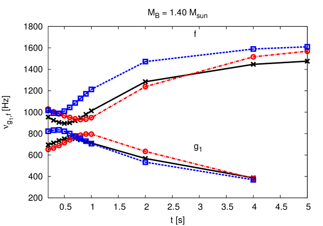
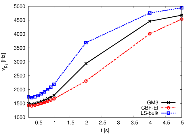
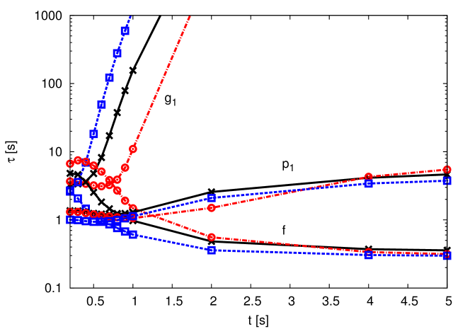
Figure 4.1: Time dependence of the PNS quasi-normal mode frequencies and damping times for the three EoSs and for $M_{\mathrm{B}}=1.40\,\mathrm{M_{\odot}}$.

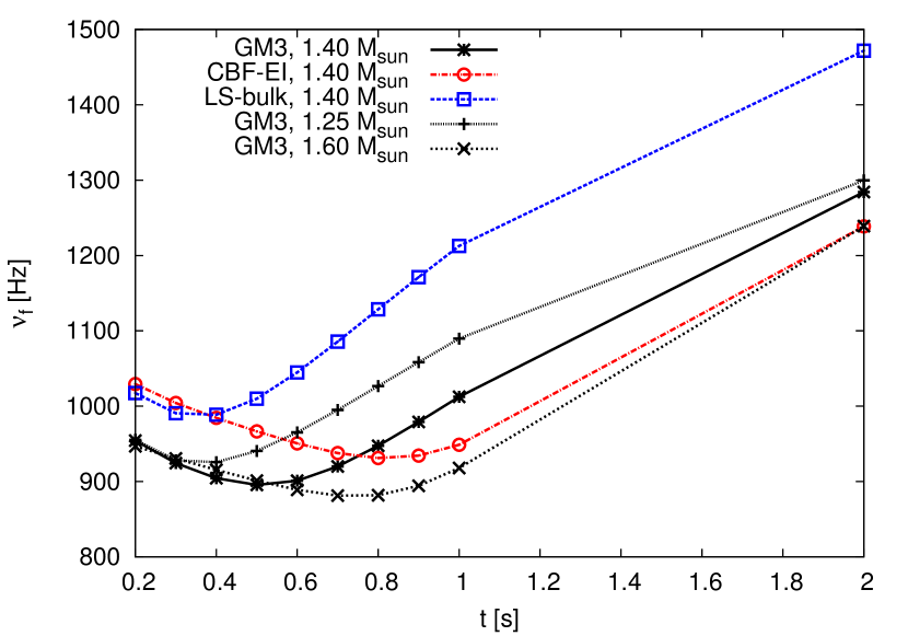
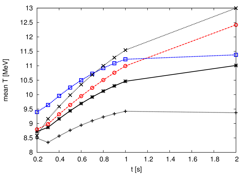
Figure 4.2: Fundamental mode frequency and mean stellar temperature for some stellar configurations from $0.2\,\mathrm{s}$ to $2\,\mathrm{s}$.

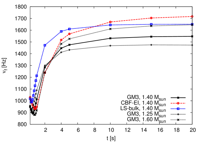
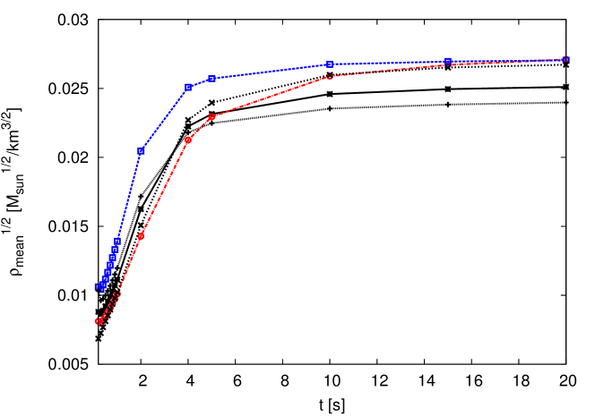
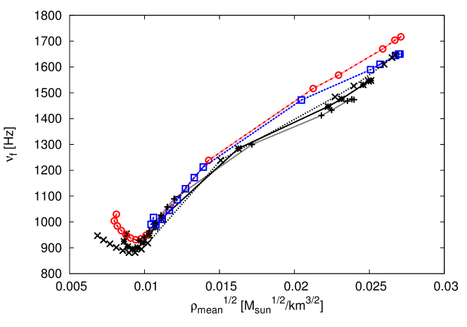
Figure 4.3: In the top plot we show the fundamental frequency evolution, in the middle plot the root square of the mean density $\sqrt{M/R^{3}}$ evolution, and in the bottom plot the fundamental density vs the root square of the mean density (the evolutionary tracks begin at the bottom left of the plot and end at $t=20\,\mathrm{s}$ at the top right).

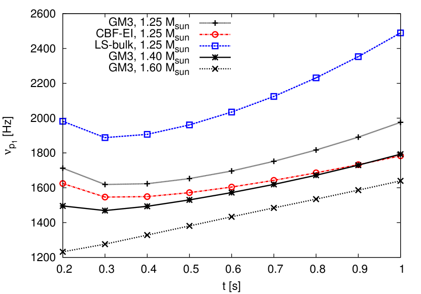
Figure 4.4: First pressure mode frequency for some stellar configurations from $0.2\,\mathrm{s}$ to $1\,\mathrm{s}$.

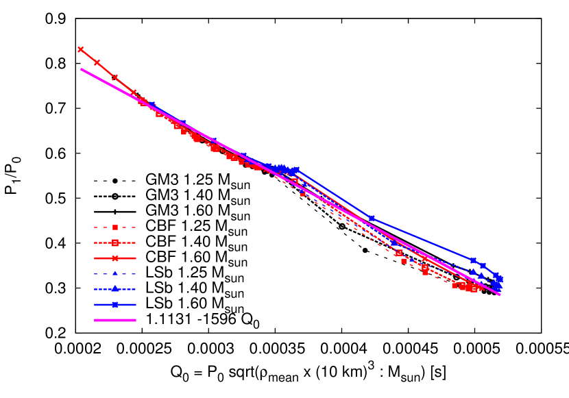
Figure 4.5: Ratio between the first p-mode period and the fundamental period as a function of the quantity $Q_{0}$, for a PNS in the configurations studied in this thesis. The points at the top-left correspond to late evolutionary times, whereas the initial configurations are in the bottom-right.

Table 4.1: QNMs for a $M_{\mathrm{B}}=1.25\,\mathrm{M_{\odot}}$ star evolved with the GM3 EoS. The column content, from left to right, is: time of the snapshot (in s), frequency (in Hz) and damping time (in s) of the $g_{1}$, $f$, and $p_{1}$ modes, stellar gravitational mass (in $M_{\odot}$), and stellar radius (in km).

$t$	$\nu_{g_{1}}$	$\tau_{g_{1}}$	$\nu_{f}$	$\tau_{f}$	$\nu_{p_{1}}$	$\tau_{p_{1}}$	$M$	$R$
0.2	784.1	4.01	955.3	2.49	1712.	1.57	1.2064	22.444
0.3	776.6	5.91	928.2	2.18	1619.	1.59	1.2051	23.530
0.4	768.0	11.5	925.7	1.75	1623.	1.56	1.2036	23.320
0.5	752.9	25.9	940.5	1.48	1653.	1.55	1.2021	22.917
0.6	734.4	58.2	965.2	1.31	1696.	1.57	1.2006	22.430
0.7	715.1	123.	995.0	1.17	1752.	1.62	1.1992	21.894
0.8	695.8	247.	1027.	1.05	1817.	1.71	1.1977	21.349
0.9	676.7	472.	1058.	.952	1890.	1.83	1.1962	20.812
1.0	658.2	873.	1090.	.869	1976.	1.98	1.1948	20.272
2.0	504.3	$1.5\times 10^{5}$	1300.	.534	3386.	3.96	1.1828	15.893
4.0	326.8	$2.8\times 10^{5}$	1412.	.446	4593.	5.96	1.1697	13.502
5.0	-	-	1433.	.434	4756.	6.46	1.1660	13.215
10.	-	-	1468.	.415	5017.	6.77	1.1562	12.778
15.	-	-	1475.	.413	5074.	6.66	1.1520	12.659
20.	-	-	1473.	.415	5091.	6.88	1.1502	12.600

Table 4.2: As Tab. 4.1, for a $M_{\mathrm{B}}=1.25\,\mathrm{M_{\odot}}$ star with the CBF-EI EoS.

$t$	$\nu_{g_{1}}$	$\tau_{g_{1}}$	$\nu_{f}$	$\tau_{f}$	$\nu_{p_{1}}$	$\tau_{p_{1}}$	$M$	$R$
0.2	756.2	3.13	1036.	4.41	1625.	1.36	1.2118	23.807
0.3	753.2	3.35	1001.	4.94	1546.	1.38	1.2102	24.808
0.4	767.0	3.47	976.8	4.45	1549.	1.34	1.2085	24.628
0.5	783.5	3.82	959.2	3.53	1572.	1.30	1.2068	24.238
0.6	796.5	4.88	950.3	2.60	1604.	1.27	1.2052	23.765
0.7	800.8	7.85	952.9	1.93	1643.	1.25	1.2035	23.251
0.8	795.4	15.4	967.7	1.55	1686.	1.25	1.2019	22.723
0.9	782.6	32.2	990.7	1.33	1732.	1.26	1.2004	22.200
1.0	766.1	66.4	1019.	1.18	1783.	1.28	1.1988	21.679
2.0	568.0	$2.5\times 10^{4}$	1296.	.556	2542.	2.32	1.1856	17.255
4.0	377.7	$3.7\times 10^{5}$	1512.	.385	4206.	6.46	1.1695	13.684
5.0	-	-	1553.	.365	4643.	7.75	1.1647	13.113
10.	-	-	1635.	.330	5355.	8.57	1.1535	12.240
15.	-	-	1659.	.321	5507.	8.04	1.1499	12.012
20.	-	-	1664.	.319	5568.	8.00	1.1492	11.903

Table 4.3: As Tab. 4.1, for a $M_{\mathrm{B}}=1.25\,\mathrm{M_{\odot}}$ star with the LS-bulk EoS.

$t$	$\nu_{g_{1}}$	$\tau_{g_{1}}$	$\nu_{f}$	$\tau_{f}$	$\nu_{p_{1}}$	$\tau_{p_{1}}$	$M$	$R$
0.2	870.3	8.57	1047.	1.21	1982.	1.23	1.2020	19.925
0.3	839.0	22.0	1045.	1.12	1888.	1.27	1.2006	20.780
0.4	805.6	62.2	1068.	1.01	1907.	1.27	1.1992	20.506
0.5	772.9	161.	1102.	.911	1961.	1.30	1.1976	20.047
0.6	742.2	380.	1139.	.821	2035.	1.37	1.1961	19.533
0.7	713.6	829.	1176.	.743	2125.	1.46	1.1946	19.003
0.8	686.9	$1.7\times 10^{3}$	1213.	.676	2231.	1.59	1.1931	18.467
0.9	662.0	$3.4\times 10^{3}$	1248.	.622	2353.	1.74	1.1917	17.948
1.0	638.7	$6.5\times 10^{3}$	1279.	.579	2490.	1.92	1.1903	17.446
2.0	473.5	$5.9\times 10^{6}$	1457.	.415	4027.	3.22	1.1789	13.939
4.0	321.8	$3.3\times 10^{5}$	1538.	.372	4864.	4.89	1.1673	12.557
5.0	278.9	$5.9\times 10^{5}$	1552.	.366	5010.	5.28	1.1638	12.378
10.	-	-	1572.	.359	5267.	6.01	1.1540	12.091
15.	-	-	1575.	.359	5328.	6.15	1.1493	12.025
20.	-	-	1575.	.360	5352.	6.22	1.1465	11.986

Table 4.4: As Tab. 4.1, for a $M_{\mathrm{B}}=1.40\,\mathrm{M_{\odot}}$ star with the GM3 EoS.

$t$	$\nu_{g_{1}}$	$\tau_{g_{1}}$	$\nu_{f}$	$\tau_{f}$	$\nu_{p_{1}}$	$\tau_{p_{1}}$	$M$	$R$
0.2	695.5	3.28	954.3	4.83	1495.	1.36	1.3553	25.961
0.3	712.6	3.38	924.5	4.62	1469.	1.35	1.3536	26.289
0.4	734.6	3.67	904.4	3.61	1494.	1.29	1.3518	25.782
0.5	751.3	4.78	895.6	2.54	1530.	1.25	1.3500	25.174
0.6	757.2	8.21	901.1	1.83	1572.	1.22	1.3482	24.560
0.7	752.5	17.2	919.9	1.46	1619.	1.21	1.3464	23.937
0.8	741.5	37.5	947.4	1.24	1672.	1.22	1.3447	23.312
0.9	727.4	78.7	979.1	1.09	1730.	1.25	1.3429	22.704
1.0	712.1	156.	1012.	.972	1793.	1.29	1.3412	22.119
2.0	567.7	$3.1\times 10^{4}$	1284.	.484	2938.	2.57	1.3260	17.122
4.0	387.1	$4.6\times 10^{6}$	1447.	.372	4461.	4.15	1.3084	13.827
5.0	-	-	1476.	.357	4678.	4.64	1.3033	13.450
10.	-	-	1531.	.335	5050.	5.14	1.2893	12.872
15.	-	-	1545.	.330	5142.	4.98	1.2827	12.725
20.	-	-	1548.	.330	5175.	4.95	1.2791	12.661

Table 4.5: As Tab. 4.1, for a $M_{\mathrm{B}}=1.40\,\mathrm{M_{\odot}}$ star with the CBF-EI EoS.

$t$	$\nu_{g_{1}}$	$\tau_{g_{1}}$	$\nu_{f}$	$\tau_{f}$	$\nu_{p_{1}}$	$\tau_{p_{1}}$	$M$	$R$
0.2	652.7	3.67	1029.	6.68	1436.	1.31	1.3613	27.434
0.3	665.1	3.60	1004.	7.48	1410.	1.31	1.3591	27.740
0.4	688.6	3.39	984.5	7.13	1430.	1.26	1.3570	27.266
0.5	715.0	3.20	966.5	6.27	1462.	1.21	1.3550	26.671
0.6	741.6	3.12	950.6	5.11	1498.	1.16	1.3529	26.044
0.7	766.0	3.25	937.7	3.84	1536.	1.12	1.3510	25.421
0.8	785.3	3.89	931.2	2.70	1578.	1.09	1.3490	24.805
0.9	795.7	5.84	934.4	1.91	1621.	1.07	1.3471	24.204
1.0	795.4	11.0	948.7	1.48	1666.	1.06	1.3453	23.622
2.0	633.8	$5.4\times 10^{3}$	1239.	.556	2308.	1.50	1.3290	18.681
4.0	381.0	$3.7\times 10^{5}$	1516.	.337	4010.	4.28	1.3079	14.254
5.0	-	-	1568.	.315	4539.	5.48	1.3013	13.520
10.	-	-	1670.	.280	5459.	7.33	1.2844	12.420
15.	-	-	1703.	.270	5674.	6.92	1.2778	12.146
20.	-	-	1717.	.266	5761.	6.69	1.2752	12.018

Table 4.6: As Tab. 4.1, for a $M_{\mathrm{B}}=1.40\,\mathrm{M_{\odot}}$ star with the LS-bulk EoS.

$t$	$\nu_{g_{1}}$	$\tau_{g_{1}}$	$\nu_{f}$	$\tau_{f}$	$\nu_{p_{1}}$	$\tau_{p_{1}}$	$M$	$R$
0.2	821.7	2.70	1017.	2.61	1739.	1.00	1.3505	22.909
0.3	832.1	3.58	990.7	2.07	1708.	.993	1.3488	23.135
0.4	834.6	6.95	988.7	1.46	1739.	.958	1.3470	22.658
0.5	821.9	18.2	1010.	1.16	1786.	.939	1.3451	22.081
0.6	800.7	49.2	1045.	.986	1846.	.938	1.3433	21.461
0.7	776.9	122.	1086.	.862	1916.	.957	1.3415	20.833
0.8	752.7	278.	1128.	.761	1996.	.996	1.3396	20.219
0.9	729.1	595.	1171.	.677	2087.	1.05	1.3379	19.615
1.0	706.3	$1.2\times 10^{3}$	1213.	.608	2190.	1.13	1.3361	19.035
2.0	533.6	$2.5\times 10^{5}$	1472.	.359	3688.	2.10	1.3214	14.668
4.0	368.9	$6.3\times 10^{7}$	1590.	.305	4757.	3.42	1.3058	12.757
5.0	-	-	1610.	.298	4946.	3.76	1.3012	12.532
10.	-	-	1644.	.288	5299.	4.41	1.2877	12.165
15.	-	-	1650.	.288	5394.	4.58	1.2807	12.082
20.	-	-	1650.	.289	5431.	4.64	1.2764	12.042

Table 4.7: As Tab. 4.1, for a $M_{\mathrm{B}}=1.60\,\mathrm{M_{\odot}}$ star with the GM3 EoS.

$t$	$\nu_{g_{1}}$	$\tau_{g_{1}}$	$\nu_{f}$	$\tau_{f}$	$\nu_{p_{1}}$	$\tau_{p_{1}}$	$M$	$R$
0.2	548.5	4.72	946.8	10.6	1232.	1.41	1.5571	32.104
0.3	587.0	4.05	930.4	9.24	1276.	1.32	1.5546	30.898
0.4	626.4	3.53	915.4	7.84	1329.	1.22	1.5522	29.722
0.5	664.1	3.18	901.1	6.38	1381.	1.14	1.5498	28.653
0.6	699.0	3.04	889.0	4.82	1433.	1.07	1.5475	27.675
0.7	728.6	3.24	881.2	3.35	1484.	1.02	1.5453	26.797
0.8	749.6	4.27	881.7	2.22	1535.	.983	1.5431	25.993
0.9	758.7	7.45	894.3	1.57	1586.	.958	1.5410	25.236
1.0	757.3	15.6	917.9	1.25	1640.	.946	1.5388	24.525
2.0	636.9	$5.4\times 10^{3}$	1239.	.464	2481.	1.46	1.5195	18.838
4.0	458.1	$6.7\times 10^{5}$	1484.	.305	4246.	2.61	1.4949	14.259
5.0	397.8	$10^{6}$	1526.	.289	4531.	3.03	1.4877	13.735
10.	-	-	1611.	.263	5050.	3.69	1.4675	12.955
15.	-	-	1636.	.256	5210.	3.62	1.4572	12.750
20.	-	-	1646.	.254	5261.	3.51	1.4509	12.665

Table 4.8: As Tab. 4.1, for a $M_{\mathrm{B}}=1.60\,\mathrm{M_{\odot}}$ star with the CBF-EI EoS.

$t$	$\nu_{g_{1}}$	$\tau_{g_{1}}$	$\nu_{f}$	$\tau_{f}$	$\nu_{p_{1}}$	$\tau_{p_{1}}$	$M$	$R$
0.2	522.7	7.45	995.1	20.4	1197.	1.41	1.5637	33.618
0.3	549.3	5.01	986.9	15.3	1231.	1.36	1.5606	32.492
0.4	581.2	4.17	978.8	12.3	1273.	1.29	1.5577	31.376
0.5	614.4	3.62	969.0	10.4	1318.	1.21	1.5551	30.341
0.6	647.5	3.21	957.7	8.95	1362.	1.14	1.5525	29.389
0.7	680.3	2.90	945.4	7.56	1408.	1.08	1.5500	28.496
0.8	711.9	2.69	933.3	6.14	1453.	1.02	1.5476	27.677
0.9	741.4	2.62	922.2	4.67	1497.	.978	1.5452	26.910
1.0	767.2	2.80	914.3	3.28	1542.	.941	1.5430	26.187
1.1	786.1	3.58	913.0	2.20	1588.	.911	1.5407	25.510
1.2	794.6	5.98	921.9	1.55	1634.	.889	1.5386	24.860
1.3	792.6	12.2	941.4	1.22	1682.	.874	1.5364	24.234
1.4	783.8	26.1	967.9	1.04	1732.	.867	1.5343	23.633
1.8	725.5	365.	1095.	.691	1957.	.910	1.5263	21.458
1.9	709.4	648.	1127.	.635	2022.	.939	1.5244	20.962
2.0	693.2	$1.1\times 10^{3}$	1158.	.586	2090.	.975	1.5226	20.486
4.0	453.8	$5.5\times 10^{5}$	1522.	.291	3758.	2.55	1.4944	14.944
5.0	-	-	1590.	.267	4348.	3.37	1.4853	14.006
10.	-	-	1714.	.233	5492.	5.69	1.4600	12.639
15.	-	-	1755.	.224	5801.	5.88	1.4485	12.295
20.	-	-	1776.	.220	5926.	5.64	1.4425	12.143

Table 4.9: As Tab. 4.1, for a $M_{\mathrm{B}}=1.60\,\mathrm{M_{\odot}}$ star with the LS-bulk EoS.

$t$	$\nu_{g_{1}}$	$\tau_{g_{1}}$	$\nu_{f}$	$\tau_{f}$	$\nu_{p_{1}}$	$\tau_{p_{1}}$	$M$	$R$
0.2	662.9	3.07	1020.	6.83	1440.	.997	1.5519	28.240
0.3	709.0	2.72	997.3	5.89	1494.	.919	1.5495	27.040
0.4	753.6	2.52	976.8	4.56	1555.	.846	1.5471	26.001
0.5	792.9	2.64	962.0	3.06	1618.	.787	1.5448	25.029
0.6	819.9	3.71	959.7	1.86	1680.	.745	1.5424	24.138
0.7	827.0	8.06	977.4	1.25	1743.	.717	1.5401	23.325
0.8	818.3	21.6	1012.	.988	1809.	.701	1.5379	22.547
0.9	802.1	55.8	1055.	.838	1879.	.699	1.5356	21.818
1.0	782.9	132.	1102.	.728	1956.	.708	1.5334	21.124
2.0	606.4	$5.3\times 10^{4}$	1473.	.315	3237.	1.24	1.5140	15.752
4.0	426.3	$1.3\times 10^{5}$	1657.	.245	4586.	2.17	1.4924	12.975
5.0	374.9	$9.2\times 10^{6}$	1687.	.237	4825.	2.44	1.4860	12.678
10.	-	-	1742.	.225	5304.	3.03	1.4670	12.201
15.	-	-	1755.	.223	5452.	3.19	1.4568	12.081
20.	-	-	1757.	.224	5510.	3.25	1.4500	12.032

Chapter 5 Rotation

In the previous chapters, we have considered a non-rotating proto-neutron star. However, when a supernova explodes, the hot, lepton-rich remnant (the proto-neutron star) is also presumably rapidly rotating. In the early stages of its evolution, the PNS cools down and loses its high lepton content, while its radius and rotation rate decrease. In this phase, a huge amount of energy and of angular momentum is released, mainly through neutrino emission (Burrows and Lattimer,, 1986; Keil and Janka,, 1995; Pons et al.,, 1999). A fraction of this energy is expected to be emitted in the gravitational wave channel; indeed, as a consequence of the violent collapse, non-radial oscillations can be excited, making PNSs promising sources for present and future gravitational detectors (Ferrari et al.,, 2003; Ott,, 2009; Burgio et al.,, 2011; Fuller et al.,, 2015). In addition, since the star rotates, if its shape deviates from axisymmetry it emits gravitational waves also due to rotation.

The study of the rotation rate evolution of a PNS during the quasi-stationary, Kelvin-Helmholtz phase is important because it allows to link the supernova explosion simulations with the observed properties of the young pulsars population. In fact, current SN simulations (see e.g. Thompson et al.,, 2005; Ott et al.,, 2006; Hanke et al.,, 2013; Couch and Ott,, 2015; Nakamura et al.,, 2014) predict that the PNS initial rotation period may be as small as few ms, whereas young pulsars have been observed with rotational periods greater than about 100 ms (see Miller and Miller,, 2014, and references therein).

The evolution of rotating PNSs has been studied in Villain et al., (2004). Villain et al., (2004) have accounted for rotation effectively, employing the thermodynamical profiles of Pons et al., (1999) (i.e., those of a non-rotating PNS evolved with the GM3 EoS) as effective time-dependent EoSs. These effective EoSs have been used to construct the rotating configurations with the non-linear BGSM code (Gourgoulhon et al.,, 1999). A similar approach has been followed in Martinon et al., (2014), which used the profiles of Pons et al., (1999) and Burgio et al., (2011). The main limitations of these works are the following.

• The evolution of the PNS rotation rate is due not only to the change of the moment of inertia (i.e., to the contraction), but also to the angular momentum change due to neutrino emission (Epstein,, 1978). This was neglected in Villain et al., (2004), and described with a heuristic formula in Martinon et al., (2014).

• As we shall discuss in this chapter, when the PNS profiles describing a non-rotating star are treated as an effective EoS, one can obtain configurations which are unstable to radial perturbations, unless particular care is taken in modelling the effective EoS.

In this chapter, we study the spin evolution of the PNS in its first tens of seconds of life, using the entropy and lepton fraction profiles obtained with the quasi-stationary evolution of a spherically symmetric PNS (Chapter 3) with the GM3 EoS, the same adopted by Villain et al., (2004). In Sec. 5.1 we describe the Hartle-Thorne equations, that we use to obtain the slowly-rotating PNS profiles. In Sec. 5.2 we describe our model to effectively include rotation in the PNS evolution; our approach is different from that used in Villain et al., (2004). In particular, we model the evolution of the angular momentum (due to neutrino emission) with the Epstein’s formula (Epstein,, 1978). In Sec. 5.3 we describe our results on the time dependence of the angular momentum and in Sec. 5.4 we discuss the gravitational wave emission which is associated with this process. The results of this chapter have been published in Camelio et al., (2016).

5.1 Slowly-rotating neutron star: the Hartle-Thorne equations

In this section, we briefly describe the equations of the perturbative Hartle-Thorne approach. For further details we refer the reader to Hartle, (1967); Hartle and Thorne, (1968); Hartle, (1973) and to the Appendix of Benhar et al., (2005).

In the Hartle-Thorne approach, the rotating star is described as a stationary perturbation of a spherically symmetric background, for small values of the angular velocity $\Omega=2\pi\nu$ (as seen by an observer at infinity), that is, for $\nu\ll\nu_{ms}$ ($\nu_{ms}$ is the mass-shedding frequency, at which the star starts losing mass at the equator, see Sec. 5.3). As shown in Martinon et al., (2014), this “slow rotation” approximation is reasonably accurate for rotation rates up to $\sim 0.8$ of the mass-shedding limit, providing values of mass, equatorial radius and moment of inertia which differ by $\lesssim 0.5\%$ from those obtained with fully relativistic, nonlinear simulations. In our approach we assume uniform rotation; PNSs are expected to have a significant amount of differential rotation at birth (Janka and Mönchmeyer,, 1989) which, however, is likely to be removed by viscous mechanisms, such as, for instance, magnetorotational instability (Mösta et al.,, 2015), in a fraction of a second. Our approach should be considered as a first step towards a more detailed description of rotating PNSs, in which we shall include differential rotation.

The spacetime metric, up to third order in $\Omega$, can be written as

$$\mathrm{d}s^{2}=-e^{2\phi(r)}\big{[}1+2h_{0}(r)+2h_{2}(r)P_{2}(\mu)\big{]}\mathrm{d}t^{2}\\ +e^{2\lambda(r)}\left[1+\frac{2m_{0}(r)+2m_{2}(r)P_{2}(\mu)}{r-2M(r)}\right]\mathrm{d}r^{2}+r^{2}[1+2k_{2}(r)P_{2}(\mu)]\\ \times\left\{\mathrm{d}\theta^{2}+\sin^{2}\theta\left[\mathrm{d}\phi-\left(\omega(r)+w_{1}(r)+w_{3}(r)P^{{}^{\prime}}_{3}(\mu)\right)\mathrm{d}t\right]^{2}\right\},$$ (5.1)

where $\mu=\cos\theta$ and $P_{n}(\mu)$ is the Legendre polynomial of order $n$, the prime denoting the derivative with respect to $\mu$. The perturbations of the non-rotating star are described by the functions $\omega$ [of $O(\Omega)$], $h_{0}$, $m_{0}$, $h_{2}$, $m_{2}$, $k_{2}$ [of $O(\Omega^{2})$], and $w_{1}$, $w_{3}$ [of $O(\Omega^{3})$]. The energy-momentum tensor is

$$T^{\mu\nu}=(\mathcal{E}+\mathcal{P})u^{\mu}u^{\nu}+\mathcal{P}g^{\mu\nu}$$ (5.2)

where $g_{\mu\nu}$, $u^{\mu}$ are the metric and four-velocity in the rotating configuration, and $\mathcal{E}$ and $\mathcal{P}$ are the energy density and pressure in the rotating star. An element of fluid, at position $(r,\theta)$ in the non-rotating star, is displaced by rotation to the position

$$\bar{r}=r+\xi(r,\theta),$$ (5.3)

where $\xi(r,\theta)=\xi_{0}(r)+\xi_{2}(r)P_{2}(\mu)+O(\Omega^{4})$ is the Lagrangian displacement. The energy and pressure Eulerian perturbations (for the difference between Eulerian and Lagrangian perturbation, see discussion in Sec. 4.1) are

$$\delta P={} \big{(}\epsilon(r)+P(r)\big{)}\big{(}\delta p_{0}(r)+\delta p_{2}(r)P_{2}(\mu)\big{)}.$$ (5.4)

$$\delta\epsilon={} \frac{\mathrm{d}\epsilon/\mathrm{d}r}{\mathrm{d}P/\mathrm{d}r}\delta P,$$ (5.5)

where $\epsilon$ and $P$ are the energy density and pressure in the non-rotating star and the perturbations depend on the functions $\delta p_{0}(r)$ and $\delta p_{2}(r)$. The background spacetime is described by the TOV equations, see Sec. 3.1.

In the Hartle-Thorne approach, one assumes that if the fluid element of the non-rotating star has pressure $P$ and energy density $\epsilon$, the displaced fluid element of the rotating star has the same values of pressure and energy density. In other words, the Lagrangian perturbations of the energy density and the pressure vanish (see Eq. (6) of Hartle,, 1967), $\Delta\epsilon=\Delta P=0$; the modification of these quantities is only due to the displacement (5.3)

$$\delta\epsilon(r,\theta)={} -\frac{\mathrm{d}\epsilon}{\mathrm{d}r}\xi(r,\theta),$$ (5.6)

$$\delta P(r,\theta)={} -\frac{\mathrm{d}P}{\mathrm{d}r}\xi(r,\theta).$$ (5.7)

We remark that as long as we neglect terms of $O(\Omega^{4})$, $\delta\epsilon(r,\theta)\simeq\delta\epsilon(\bar{r},\theta)$.

Einstein’s equations, expanded in powers of $\Omega$ and in Legendre polynomials, can be written as a set of ordinary differential equations for the perturbation functions. The spacetime perturbation to first order in $\Omega$ is described by the function $\omega(r)$, which is responsible for the dragging of inertial frames; it satisfies the equations

$$\frac{\mathrm{d}\chi}{\mathrm{d}r}={} \frac{u}{r^{4}}-\frac{4\pi r^{2}(\epsilon+P)\chi}{r-2M},$$ (5.8)

$$\frac{\mathrm{d}u}{\mathrm{d}r}={} \frac{16\pi r^{5}(\epsilon+P)\chi}{r-2M},$$ (5.9)

where $M$ is the gravitational mass of the non-rotating star (obtained with the TOV equations), $\varpi=\Omega-\omega$, $j(r)=e^{-\phi}\sqrt{1-2M/r}$, $\chi=j\varpi$ and $u=r^{4}jd\varpi/dr$. The angular momentum $J$ is obtained by matching the interior with the exterior solution $\chi(r)=\Omega-2J/r^{3}$, $u(r)=6J$ at $r=R$. The moment of inertia, at zero-th order in the rotation rate, is $I=J/\Omega$. The perturbations to second order in $\Omega$ are described by the metric functions $h_{l}(r)$, $m_{l}(r)$ ($l=0,2$), $k_{2}(r)$, and by the fluid pressure perturbations $\delta p_{l}$. The $l=0$ perturbations satisfy the equations

$$\frac{\mathrm{d}}{\mathrm{d}r}\left(\delta p_{0}+h_{0}-\frac{\chi^{2}r^{3}}{3(r-2M)}\right)={} 0,$$ (5.10)

$$\delta p_{2}+h_{2}-\frac{\chi^{2}r^{3}}{3(r-2M)}={} 0,$$ (5.11)

$$\frac{\mathrm{d}m_{0}}{\mathrm{d}r}={} 4\pi r^{2}\frac{\mathrm{d}\epsilon}{\mathrm{d}P}[\delta p_{0}(\epsilon+P)]+\frac{u^{2}}{12r^{4}}+\frac{8\pi r^{5}(\epsilon+P)\chi^{2}}{3(r-2M)},$$ (5.12)

$$\frac{\mathrm{d}\delta p_{0}}{\mathrm{d}r}={} \frac{u^{2}}{12r^{4}(r-2M)}-\frac{m_{0}(1+8\pi r^{2}P)}{(r-2M)^{2}}-\frac{4\pi(\epsilon+P)r^{2}\delta p_{0}}{r-2M}$$

$$+\frac{2r^{2}\chi}{3(r-2M)}\left[\frac{u}{r^{3}}+\frac{(r-3M-4\pi r^{3}P)\chi}{r-2M}\right].$$ (5.13)

Matching the interior and the exterior solutions at $r=R$ ($R$ is the radius of the non-rotating star), it is possible to compute the monopolar stellar deformation, and then the correction to the gravitational mass due to stellar rotation, $\delta M=m_{0}(R)+J^{2}/R^{3}$. The baryonic mass correction $\delta M_{B}=\delta m_{B}(R)$ is found by solving the equation

$$\frac{\mathrm{d}\delta m_{B}}{\mathrm{d}r}=4\pi r^{2}e^{\lambda}\left[\left(1+\frac{m_{0}}{r-2m}+\frac{1}{3}r^{2}\varpi^{2}e^{-2\phi}\right)\epsilon+\frac{\mathrm{d}\epsilon/\mathrm{d}r}{\mathrm{d}P/\mathrm{d}r}(\epsilon+P)\delta p_{0}\right].$$ (5.14)

The $l=2$ perturbations satisfy the equations

$$\frac{\mathrm{d}v_{2}}{\mathrm{d}r}={} -2\frac{\mathrm{d}\phi}{\mathrm{d}r}h_{2}+\left(\frac{1}{r}+\frac{\mathrm{d}\phi}{\mathrm{d}r}\right)\left[\frac{8\pi r^{5}(\epsilon+P)\chi^{2}}{3(r-2M)}+\frac{u^{2}}{6r^{4}}\right],$$ (5.15)

$$\frac{\mathrm{d}h_{2}}{\mathrm{d}r}={} \left[-2\frac{\mathrm{d}\phi}{\mathrm{d}r}+\frac{r}{r-2M}\left(2\frac{\mathrm{d}\phi}{\mathrm{d}r}\right)^{-1}\left(8\pi(\epsilon+P)-\frac{4M}{r^{3}}\right)\right]h_{2}$$

$$-\frac{4v_{2}}{r(r-2M)}\left(2\frac{\mathrm{d}\phi}{\mathrm{d}r}\right)^{-1}+\frac{u^{2}}{6r^{5}}\left[\frac{\mathrm{d}\phi}{\mathrm{d}r}r-\frac{1}{r-2M}\left(2\frac{\mathrm{d}\phi}{\mathrm{d}r}\right)^{-1}\right]$$

$$+\frac{8\pi r^{5}(\epsilon+P)\chi^{2}}{3(r-2M)}\left[\frac{\mathrm{d}\phi}{\mathrm{d}r}r+\frac{1}{r-2M}\left(2\frac{\mathrm{d}\phi}{\mathrm{d}r}\right)^{-1}\right],$$ (5.16)

where $v_{2}=k_{2}+h_{2}$. Matching the interior and the exterior solutions, it is possible to determine the quadrupole deformation of the PNS and then the quadrupole moment.

The equations for the peturbations at $O(\Omega^{3})$, $w_{l}(r)$ ($l=1,3$), have a similar structure but they are longer and are not reported here; we refer the reader to Hartle, (1973) and the Appendix of Benhar et al., (2005). They yield the octupole moment, the third-order corrections to the angular momentum and the second-order corrections to the moment of inertia.

For each value of the central pressure $P_{c}$ (or, equivalently, of the central energy density $\epsilon_{c}$) and of the rotation rate $\Omega$, the numerical integration of the perturbation equations yields the perturbation functions, and then the values of the multipole moments of the star (in particular, the gravitational mass of the rotating star $M^{\mathrm{rot}}$ and the angular momentum $J$), and of its baryonic mass $M^{\mathrm{rot}}_{\mathrm{B}}$. These quantities can be written as $M^{\mathrm{rot}}=M+\delta M$, $J=\delta J$, $M^{\mathrm{rot}}_{\mathrm{B}}=M_{\mathrm{B}}+\delta M_{B}$, etc., where the quantities with superscript ^rot refer to the rotating star. Given a non-rotating star with central pressure $P_{c}$, gravitational mass $M$, and baryon mass $M_{\mathrm{B}}$, the rotating star (with spin $\Omega$) with the same central pressure has a baryon mass $M_{\mathrm{B}}+\delta M_{B}$, which is generally larger than $M_{\mathrm{B}}$. Therefore, a rotating star with the same baryon mass $M_{\mathrm{B}}$ as the non-rotating one, has necessarily a smaller value of the central pressure, $P_{c}+\delta P_{c}$, with $\delta P_{c}<0$ (this is not surprising: when a star is set into rotation, its central pressure decreases).

5.2 Including the rotation in an effective way

In this section we describe how we account for slow rotation in the evolution of the PNS.

In order to integrate the structure equations of the PNS we need to assign an equation of state which is non-barotropic, thus we also need to know the profiles of entropy and lepton fraction throughout the star (see discussion in Secs. 2.7 and 3.1). As discussed in Chapter 3, these profiles are obtained by our evolutionary code for a spherical, non-rotating PNS at selected values of time.

The non-rotating profiles can be used to compute the structure of a rotating PNS in different ways. A possible approach is the following. Let us consider a spherical PNS with baryon mass $M_{B}$ at a given evolution time $t$. The numerical code discussed in Chapter 3 provides the functions $P(a)$, $\epsilon(a)$, $s(a)$, $Y_{L}(a)$, where we remind that $a$ is the enclosed baryon number. If we replace the inverse function of $P(a)$ into the non-barotropic EoS, we obtain an “effective barotropic EoS”, $\tilde{\epsilon}(P)=\epsilon(P,s(a(P)),Y_{L}(a(P))$, which can be used to solve the TOV equations for the spherical configuration to which we add the perturbations due to rotation, according to Hartle’s procedure. Since the rotating star must have the same baryon mass as the spherical star, one can proceed as follows: (i) solve the TOV equations for a spherically symmetric star with central pressure $P_{c}+\delta P_{c}$; (ii) solve the perturbation equations for a chosen value of the rotation rate, to determine the actual baryon mass of the rotating star with that central pressure; (iii) iterate these two steps modifying $\delta P_{c}$ until the baryon mass coincides with the assigned value $M_{B}$. This approach was used in Villain et al., (2004), where the rotating star was modeled solving the fully non-linear Einstein equations.

However, this procedure has some relevant drawbacks. Indeed, during the first second after bounce the star is very weakly bound, and it may happen that the procedure above yields $\delta P_{c}>0$, which indicates that these configurations are in the unstable branch of the mass-radius diagram. We think that this is caused by the nonphysical treatment (effective, as a barotropic EoS) of the thermodynamical profile. This problem did not occur in the simulations of Villain et al., (2004) because the authors considered a different, stable branch of the mass-radius curve corresponding to the “effective” EoS $\tilde{\epsilon}(P)$, at much lower densities. Indeed, for $t\lesssim 0.5$ s, at the center of the star they had $n_{B}\sim 10^{-2}\,\mathrm{fm^{-3}}$ (i.e., rest-mass density $\rho\sim 10^{13}\,\mathrm{g/cm^{3}}$), which corresponds to the outer region of the star modeled in Pons et al., (1999). When the central density is so low, only a small region of the star is described by the GM3 EoS; the rest is described by the low-density EoS used to model the PNS envelope, which does not yield unstable configurations.

Since we want to model the PNS consistently with the evolutionary models, we decided to implement the non-rotating profiles in an alternative way. As in the previous approach, we consider the spherical configuration obtained by the evolution code at time $t$, with central density $P_{c}$ and baryon mass (constant during the evolution) $M_{B}$. To describe the rotating star, we use the GM3 EoS $\epsilon=\epsilon(P,s,Y_{L})$; since we are restricting our analysis to slowly rotating stars, the entropy and lepton fraction profiles $s(a)$ and $Y_{L}(a)$ of the non-rotating star are a good approximation for those of the rotating star. We follow the steps discussed before: (i) solve the TOV equations for a star with central pressure $P_{c}+\delta P_{c}$; at each value of $a$, the energy density is $\epsilon(P,s(a),Y_{L}(a))$; (ii) solve Hartle’s perturbation equations, finding the baryon mass of the star rotating to a given rate with this reduced central pressure and find the correction to the baryon mass due to rotation; (iii) iterate the first two steps, finding $\delta P_{c}$ such that the baryon mass of the rotating star is $M_{B}$. We remark that the energy density of the rotating star in step (ii) is related to that of the non-rotating star in step (i) by the Hartle-Thorne prescription described above Eq. (5.6). Since we are using an appropriate non-barotropic EoS, the instability discussed above disappears, and the central pressure of the rotating star is, as expected, always smaller than that of the non-rotating star with the same baryon mass. However, the central density is high enough for the most of the star to be described by the GM3 EoS.

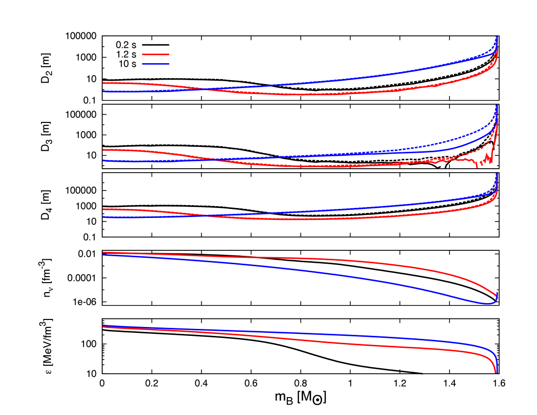
Figure 5.1: Neutrino diffusion coefficients $D_{n}$ ($n=2,3,4$), as functions of the enclosed baryon mass, computed using the density and thermodynamical profiles of the non-rotating (solid line) and rotating (dashed line) configurations, at $t=0.2$ s, $t=1.2$ s and $t=10$ s (upper and middle panels). Profiles of neutrino number density and energy density (lower panels). We assume $M_{B}=1.6\,M_{\odot}$ and that the angular momentum is the maximum allowed $J_{in}=J_{max}$ (for $J_{in}>J_{max}$, the PNS reaches the mass-shedding limit during its evolution, see Sec. 5.3).

We stress again that we are using the numerical solution of the transport equations for a non-rotating PNS, to build quasi-stationary configurations of a rotating PNS. Therefore, we are neglecting the effect of rotation on the time evolution of the PNS. To be consistent, we should have integrated the transport equations appropriate for a rotating star, which are much more complicated. Since these approximations affect the timescale of the stellar evolution, we would like to estimate how faster, or slower, the rotating star loses its thermal and lepton content with respect to the non-rotating one. Since the evolution timescale is governed by neutrino diffusion processes, at each time step of the non-rotating PNS evolution, we have computed and compared the neutrino diffusion coefficients $D_{n}$ [see Eqs. (3.102) and (3.103)] for non-rotating and rotating configurations. The latter have been obtained by replacing the profiles ($P(a)$, $\epsilon(a)$, etc.) of a non-rotating PNS with those of a rotating PNS (computed as discussed above in this Section). In the upper and middle panels of Fig. 5.1 we plot $D_{2},D_{3}$ and $D_{4}$ as functions of the enclosed baryon mass $m_{B}=m_{n}a$ ($m_{n}$ is the neutron mass), for the non-rotating (solid line) and rotating (dashed line) configurations, at $t=0.2$ s, $t=1.2$ s and $t=10$ s. In the lower panels we plot the neutrino number density and the total energy density at the same times. We set $M_{B}=1.6\,M_{\odot}$ and that the initial angular momentum, $J_{in}$, is equal to the maximum angular momentum $J_{max}$, above which mass-shedding sets in (see Sec. 5.3 for further details). We see that the diffusion coefficients of the rotating configurations are larger than those of the non-rotating star. For $m_{B}\lesssim 1\leavevmode\nobreak\ M_{\odot}$ the relative difference $|D_{n}^{\mathrm{rot}}-D_{n}^{\mathrm{non\leavevmode\nobreak\ rot}}|/|D_{n}^{\mathrm{non\leavevmode\nobreak\ rot}}|$ is always smaller than $\sim 10-20\%$, and becomes smaller than a few percent after the first few seconds. In the outer region $m_{B}\gtrsim 1\leavevmode\nobreak\ M_{\odot}$ and early times, the relative difference seems larger, in particular for the coefficient $D_{3}$, but this has no effect for two reasons: first, as shown in the two lower panels of Fig. 5.1, both the neutrino number density and the total energy density are much smaller than in the inner core; therefore, even though the diffusion coefficients of the rotating star are larger than those of the non-rotating one, few neutrinos are trapped in this region and transport effects do not contribute significantly to the overall evolution; second, the differences become large in the semi-transparent region, when the mean free path becomes comparable to (or larger than) the distance to the star surface. In this region the diffusion approximation breaks down and in practice the diffusion coefficients are always numerically limited by the flux-limiter (see Sec. 3.4).

From the above discussion we can conclude that the rotating star loses energy and lepton number through neutrino emission faster than the non-rotating one. This effect is larger at the beginning of the evolution, that is for $t\lesssim 2$ s, and is of the order of $\sim 10-20\%$, but becomes negligible at later times. Consequently our rotating star cools down and contracts over a timescale which, initially, is $\sim 10-20\%$ shorter than that of the corresponding non-rotating configuration.

Once the equations describing the rotating configuration are solved for each value of the evolution time $t$ and for an assigned value of the rotation rate $\Omega$, the solution of these equations allows one to compute the multipole moments of the rotating star, including the angular momentum $J$. Conversely we can choose, at each value of $t$, the value of the angular momentum, and determine, using a shooting method, the corresponding value of the rotation rate.

If we want to describe the early evolution of a rotating PNS, we need a physical prescription for the time dependence of $J$. For instance, we may assume that the angular momentum is constant, as in Villain et al., (2004) (see also Goussard et al.,, 1997, 1998). However, in the first minute of a PNS life, neutrino emission carries away $\sim 10\%$ of the star gravitational mass (Lattimer and Prakash,, 2001), and also a significant fraction of the total angular momentum (Janka,, 2004). To our knowledge, the most sensible estimate of the neutrino angular momentum loss in PNSs has been done in Epstein, (1978)

$$\frac{dJ}{dt}=-\frac{2}{5}qL_{\nu}R^{2}\Omega,$$ (5.17)

where $R$ is the radius of the star, $L_{\nu}=-\mathrm{d}M/\mathrm{d}t$ is the neutrino energy flux, and $q$ is an efficiency parameter, which depends on the features of the neutrino transport and emission. If neutrinos escape without scattering, $q=1$; if, instead, they have a very short mean free path, they are diffused up to the surface, and then are emitted with $q=5/3$. As discussed in Epstein, (1978) (see also Kazanas,, 1977; Mikaelian,, 1977; Henriksen and Chau,, 1978), $q=5/3$ should be considered as an upper limit of the angular momentum loss by neutrino emission. A more recent, alternative study (Dvornikov and Dib,, 2010) indicates an angular momentum emission smaller than this limit. In the following, we shall consider Epstein’s formula with $q=5/3$, and this has to be meant as an upper limit. We also mention that a simplified expression based on Epstein’s formula for the angular momentum loss in PNSs has been derived in Janka, (2004) and used in Martinon et al., (2014).

We mention that in O’Connor and Ott, (2010) the neutrino transport equations for a rotating star in general relativity have been solved by using an alternative approach. In this approach (which is believed to be accurate for slowly rotating stars, O’Connor and Ott,, 2010) the structure and transport equations for a spherically symmetric star are modified by adding a centrifugal force term, to include the effect of rotation.

5.3 Results: spin evolution of the proto-neutron star

In Figure 5.2 we show how the angular momentum changes according to Epstein’s formula (5.17) as the PNS evolves. We assume $q=5/3$ and baryonic mass $M_{B}=1.6\,M_{\odot}$. We consider different values of the angular momentum $J_{in}$ at the beginning of the quasi-stationary phase ($t=0.2$ s after the bounce): $J_{in}=2.02\times 10^{48}\,\mathrm{erg\,s}$, $J_{in}=3.71\times 10^{48}\,\mathrm{erg\,s}$ and $J_{in}=8.08\times 10^{48}\,\mathrm{erg\,s}$. We find that, in the first ten seconds after bounce, $13\%$ of the initial angular momentum is carried away by neutrinos if $J_{in}=2.02\times 10^{48}\,\mathrm{erg\,s}$ or $J_{in}=3.71\times 10^{48}\,\mathrm{erg\,s}$; $20\%$ of the initial angular momentum is carried away if $J_{in}=8.075\times 10^{48}\,\mathrm{erg\,s}$. As mentioned above, $q=5/3$ should be considered as an upper bound; for smaller values of $q$, the rate of angular momentum loss would be smaller.

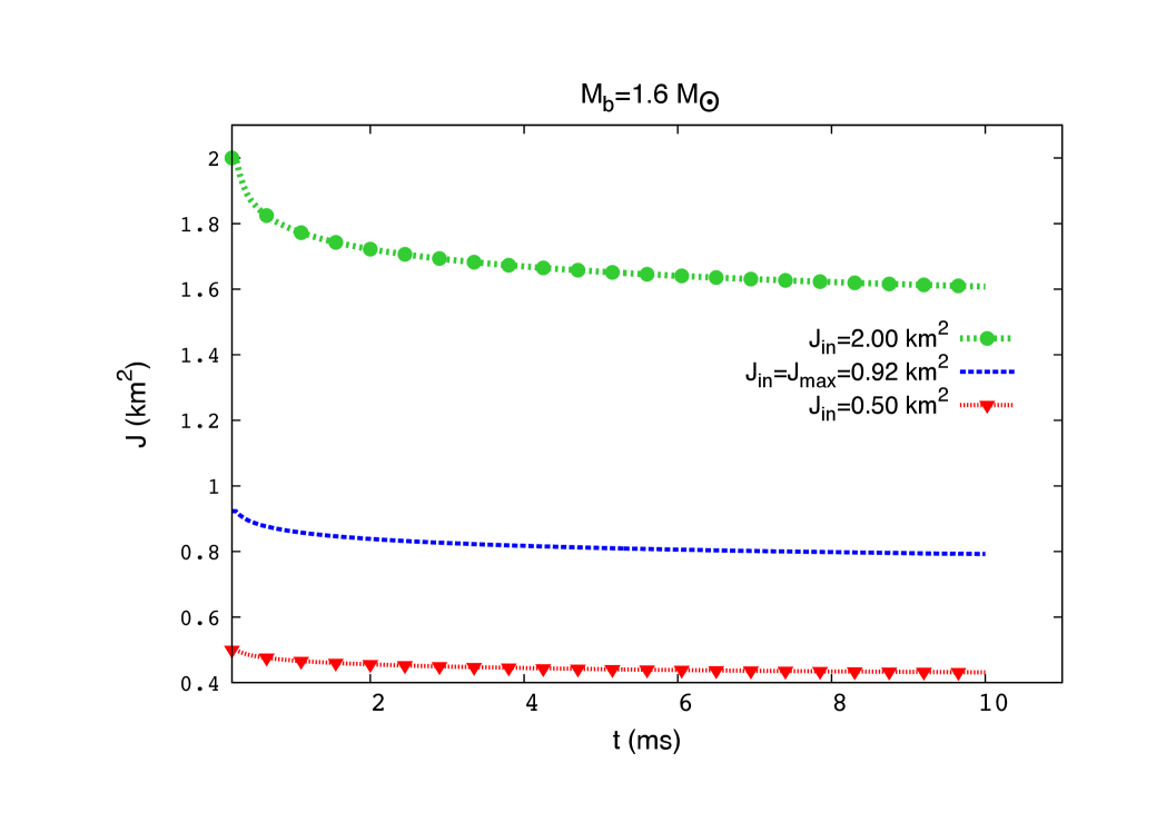
Figure 5.2: Angular momentum evolution due to neutrino losses, for a PNS with baryonic mass $M_{B}=1.6\,M_{\odot}$ and initial angular momentum $J_{in}=(2.02,\,3.71,\,8.08)\times 10^{48}$erg s.

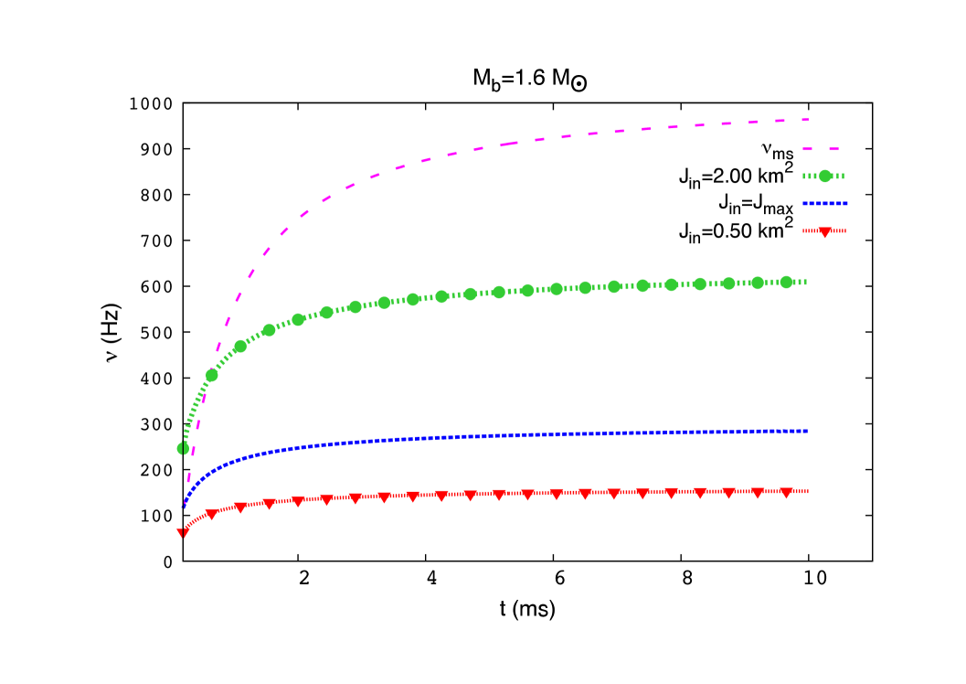
Figure 5.3: Evolution of the PNS rotation rate, corresponding to the angular momentum profiles shown in Figure 5.2.

The corresponding evolution of the PNS rotation frequency is shown in Figure 5.3. In the same Figure we also show the mass-shedding frequency $\nu_{ms}$ determined using a numerical fit derived in Doneva et al., (2013) from fully relativistic, non-linear integration of Einstein’s equations:

$$\nu_{ms}(Hz)=a\sqrt{\frac{M/M_{\odot}}{R/1{\rm km}}}+b$$ (5.18)

where $a=45862$ Hz and $b=-189$ Hz. We remark that the coefficients $a,b$ of this fit do not depend on the EoS. We see that if $J_{in}=8.08\times 10^{48}\,\mathrm{erg\,s}$, the curves of $\nu(t)$ and of $\nu_{ms}(t)$ cross during the quasi-stationary evolution; before the crossing, the PNS spin is larger than the mass-shedding limit. This means that a PNS with such initial angular momentum would lose mass. If we require the initial rotation rate to be smaller than the mass-shedding limit, we must impose $J_{in}\leq J_{max}\equiv 3.72\times 10^{48}\,\mathrm{erg\,s}$. We remark that the value of $J_{max}$ is not affected by the efficiency of angular momentum loss $q$: if $q<5/3$, $J_{max}$ has the same value, but the rotation rate grows more rapidly than in Figure 5.3.

It is interesting to note that, since $\nu_{ms}$ has a steeper increase than $\nu(t)$, even when the bound $\nu\leq\nu_{ms}$ is saturated at the beginning of the quasi-stationary phase the frequency becomes much smaller than the mass shedding frequency at later times. This is an a-posteriori confirmation that the slow rotation approximation is appropriate to study newly born PNSs. For $t>10$ s, the PNS radius does not change significantly, and the star starts to spin down due to electromagnetic and gravitational emission. However this spin down timescale is much longer than the timescale of the quasi-stationary evolution we are considering; therefore it is unlikely that after this early phase the PNS rotation rate is larger than $\sim 300$ Hz (i.e., that its period is smaller than $\sim 3$ ms), unless some spin-up mechanism (such as e.g. accretion) sets in. A less efficient angular momentum loss ($q<5/3$) would moderately increase this final value, but the general picture would remain the same.

It is worth noting that models of pre-supernova stellar evolution (Heger et al.,, 2005) predict a similar range of the PNS rotation rate and angular momentum. Among the models considered in Heger et al., (2005), the only one with $J>J_{max}$ (and rotation period smaller than $3$ ms) is expected to collapse to a black hole. Other works (Thompson et al.,, 2005; Ott et al.,, 2006) have shown that if the progenitor has a rotation rate sufficiently large, the PNS resulting from the core-collapse can have periods of few ms; our results suggest that this scenario is unlikely, unless there is a significant mass loss in the early Kelvin-Helmoltz phase.

5.4 Results: gravitational wave emission

If the evolving PNS is born with some degree of asymmetry, it emits gravitational waves. Assuming that the star rotates about a principal axis of the moment of inertia tensor, that is, that there is no precession, gravitational waves are emitted at twice the orbital frequency $\nu$, with amplitude (Zimmermann and Szedenits,, 1979; Thorne,, 1987; Bonazzola and Gourgoulhon,, 1996; Jones,, 2002)

$$h_{0}\simeq{} \frac{4G(2\pi\nu)^{2}I_{3}\varepsilon}{c^{4}d},$$ (5.19)

$$\varepsilon={} \frac{I_{1}-I_{2}}{I_{3}},$$ (5.20)

where $G$ is the gravitational constant, $c$ the speed of light, $d$ the distance from the detector, and the deviation from axisymmetry is described by the ellipticity $\varepsilon$. $I_{1}$, $I_{2}$, and $I_{3}$ are the principal moments of inertia of the PNS and $I_{3}$ is assumed to be aligned with the rotation axis. For old neutron stars, the loss of energy through gravitational waves is compensated by a decrease of rotational energy, which contributes to the spin-down of the star (the main contribution to the spin-down being that of the magnetic field).

In the case of a newly born PNS, the situation is different. As the star contracts, due to the processes related to neutrino production and diffusion, its rotation rate increases. If the PNS has a finite ellipticity, it emits gravitational waves, whose amplitude and frequency also increase as the star spins up. The timescale of this process is of the order of tens of seconds. In our model, for simplicity we shall assume that the PNS ellipticity remains constant over this short time interval.

Unfortunately, the ellipticity of a PNS is unknown. In cold, old NSs it is expected to be, at most, as large as $\sim 10^{-5}-10^{-4}$ (Haskell et al.,, 2006; Ciolfi et al.,, 2010) (larger values are allowed for EoSs including exotic matter phases, Horowitz and Kadau,, 2009; Johnson-McDaniel and Owen,, 2013). For newly born PNSs, it may be larger, but we have no hint on its actual value. To our knowledge, current numerical simulations of core-collapse do not provide estimates of the PNS ellipticity. We remark that although there is observational evidence of large asymmetries in supernova explosions (Wang et al.,, 2003; Leonard et al.,, 2006), there is no evidence that they can be inherited by the PNS. In the following, we shall assume $\varepsilon=10^{-4}$, but this should be considered as a fiducial value: the gravitational wave amplitude (which is linear in $\varepsilon$) can be easily rescaled for different values of the PNS ellipticity.

If the PNS has a finite ellipticity $\varepsilon$ it emits gravitational waves with frequency $f(t)=2\nu(t)$ and amplitude given by Eq. (5.19), with $\nu\equiv\nu(t)$ and $I_{3}\equiv I_{3}(t)$. As the spin rate $\nu(t)$ increases, both the frequency and the amplitude of the gravitational wave increase; therefore, the signal is a sort of “chirp”; this is different from the chirp emitted by neutron star binaries before coalescence, because the amplitude increases at a much milder rate and the frequency migrates at a rate which depends on the evolutionary timescale. In Figure 5.4 we show the strain amplitude $\tilde{h}(f)\sqrt{f}=\sqrt{f}\sqrt{(\tilde{h}_{+}(f)^{2}+\tilde{h}_{\times}(f)^{2})/2}$, where $\tilde{h}_{+,\times}(f)$ are the Fourier transform of the two polarization of the gravitational wave signal

$$h_{+}={} h_{0}\frac{1+\cos^{2}i}{2}\cos\big{(}2\pi f(t)t\big{)},$$ (5.21)

$$h_{\times}={} h_{0}\cos i\sin\big{(}2\pi f(t)t\big{)},$$ (5.22)

and $i$ is the angle between the rotation axis and the line of sight. In Fig. 5.4 the signal strain amplitude, computed assuming optimal orientation, $J_{in}=J_{max}$, $\varepsilon=10^{-4}$, and a distance of $r=10$ kpc, is compared with the sensitivity curves of Advanced Virgo, Advanced LIGO, and of the third generation detector ET. We see that the signal is marginally above noise for the advanced detectors, but it is definitely above the noise curve for ET. This signal would be seen by Advanced Virgo with a signal-to-noise ratio $\mathrm{SNR}=1.4$, and by Advanced LIGO with $\mathrm{SNR}=2.2$, too low to extract it from the detector noise; however, since the signal-to-noise ratio scales linearly with the ellipticity, a star born with $\varepsilon=10^{-3}$ would be detected with $\mathrm{SNR}=14$ and $\mathrm{SNR}=22$ by Advanced Virgo and LIGO, respectively. The third generation detectors like ET would detect the signal coming from a galactic PNS born with $\varepsilon=10^{-4}$ with a very large signal-to-noise ratio, i.e. $\mathrm{SNR}=22$. If the source is in the Virgo cluster ($d=15\,\mathrm{Mpc}$), the ellipticity of the PNS should be as large as $5\cdot 10^{-2}$ to be seen by ET with $\mathrm{SNM}=8$.

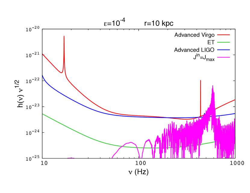
Figure 5.4: The strain amplitude $\tilde{h}(f)\sqrt{f}$ of the gravitational wave signal emitted by a PNS with $\epsilon=10^{-4}$, $J_{in}=J_{max}$, at a distance $r=10$ kpc, is compared with the noise curves of Advanced Virgo, Advanced LIGO and ET.

Chapter 6 Conclusions and outlook

In this thesis we have studied the evolution and the gravitational wave emission of a proto-neutron star in the Kelvin-Helmoltz phase, that is the period of the neutron star life subsequent to the supernova explosion, until the star becomes transparent to neutrinos. This phase lasts for tens of seconds and its beginning may be placed at about 200 ms after core bounce. The evolution can be modeled as a sequence of quasi-stationary configurations in which the matter is almost in beta-equilibrium (Burrows and Lattimer,, 1986). To perform this study, we have written a new general relativistic, one-dimensional, energy-averaged, and flux-limited PNS evolutionary code which evolves a general EoS consistently. In particular, we have considered three nucleonic equation of states and three stellar masses, and we have determined the neutrino cross sections self-consistently with the corresponding EoS. The EoSs considered are all nucleonic (without hyperons) and are obtained (i) by the extrapolation of the nuclear matter properties determined by terrestrial experiments (the LS-bulk EoS, Lattimer and Swesty,, 1991) (ii) by the nuclear relativistic mean-field theory (the GM3 EoS, Glendenning and Moszkowski,, 1991) (iii) by the nuclear non-relativistic many-body and effective interaction theory (the CBF-EI EoS, Benhar and Lovato,, 2017; Lovato et al., ming, forthcoming). We have determined the frequencies of the quasi-normal oscillation modes for the different EoSs and stellar masses (Camelio et al.,, 2017) and we have studied the angular momentum evolution and the gravitational wave emission of the proto-neutron star in the case of the GM3 mean-field EoS, including rotation in an effective way (Camelio et al.,, 2016).

The main improvements with respect to previous works introduced by our study are the following.

• We have developed and tested a new fitting formula for the interacting part of the baryon free energy (i.e., neutrons plus protons), which is valid for high density matter, finite temperature, and intermediate proton fractions. We used this fitting formula to derive the other thermodynamical quantities. This formula is suitable to be used in evolutionary codes.

• We have computed the neutrino cross sections for the many-body theory EoS of Benhar and Lovato, (2017). They have been computed at the mean-field level (Reddy et al.,, 1998), that is, the interaction between baryons has been accounted for modifying the baryon energy spectra by means of density-, temperature-, and composition-dependent effective masses and single particle energies.

• We used these neutrino cross sections to evolve the PNS with the many-body EoS in a consistent way. To our knowledge, this is the first time that a PNS with a many-body EoS has been evolved with consistently determined neutrino opacities. From this evolution, we have determined the stellar quasi-normal modes.

• We have adopted a new method to account for rotation in an effective way, namely we have used a time-dependent effective EoS which depends on the enclosed baryon mass, instead of on the pressure like Villain et al., (2004). Our method has the advantage to avoid nonphysical instabilities in the procedure adopted to include rotation.

• We have consistently accounted for angular momentum loss by neutrino emission, using the Epstein formula (Epstein,, 1978). Earlier, the angular momentum was assumed to be constant (Villain et al.,, 2004) or it was modeled with a heuristic formula (Martinon et al.,, 2014).
  

The main results of this thesis are the following.

• The PNS evolution depends on the adopted EoS. In particular, for the many-body EoS CBF-EI the PNS cooling is faster than that with the mean-field EoS GM3, which in turn is faster than that with the extrapolated EoS LS-bulk. We explain this with the fact that in the CBF-EI many-body theory the interaction between baryons is stronger than in the GM3 mean-field theory (in fact, the baryon masses are smaller in the CBF-EI than in the GM3 EoS). In the extrapolated EoS LS-bulk the effective baryon masses have been assumed equal to the bare ones, and the result is that, for what regards the computation of the neutrino cross sections, this EoS is “less interacting” than the others.

• The deleptonization of the PNS with the CBF-EI EoS is almost completed at the end of the Joule-heating phase (similarly to what was found in the first PNS numerical studies by Burrows and Lattimer,, 1986 and Keil and Janka,, 1995), whereas the deleptonization for the GM3 and LS-bulk EoSs proceeds during the cooling phase (as found by Pons et al.,, 1999). Pons et al., (1999) explained the difference in the duration of the deleptonization with the over-simplifications in the treatment of the neutrino opacities in the first works of Burrows and Lattimer, (1986) and Keil and Janka, (1995). However, we compute the neutrino cross sections for the CBF-EI and the other EoSs with the same procedure of Pons et al., (1999). Therefore, the faster deleptonization is a feature due also to the EoS properties and not only to the treatment of neutrino opacities.

• The total number of electron antineutrinos detected depends on the gravitational binding energy but is not completely determined by it. In particular, the CBF-EI EoS has more antineutrino detected than the LS-bulk EoS, even though its binding energy is smaller. This is due to the fact that the CBF-EI has higher temperatures than the other EoSs, hence the electron antineutrino distribution function at the neutrinosphere is smother and more antineutrino have energies larger than the detector energy threshold at the detector. This result remarks the importance of an accurate modeling of the PNS evolution in order to extract information on the PNS physics from the neutrino signal.

• We show that during the first second, the frequencies at which the PNS oscillates emitting gravitational waves have a non monotonic behaviour. The fundamental mode frequency decreases, reaches a minimum and then increases toward the value corresponding to the cold neutron star which forms at the end of the evolution. The frequency of the first $g$ mode increases, reaches a maximum and then decreases to the asymptotic zero limit, that of the mode $p_{1}$ has a less pronounced minimum at earlier times with respect to the $f$ mode. We show that this behaviour, already noted in Ferrari et al., (2003) for the EoS GM3 for the $f$ and $g_{1}$ modes, is a generic feature when the PNS evolution is consistently described, and that the timescale depends on the EoS. Indeed the time needed to reach the minimum (maximum) for the $f$- ($g_{1}$-) mode can differ by as much as half a second for the EoS we consider.

  During the first second, the damping time of all modes is shorter than the neutrino diffusive timescale ($\sim 10\,\mathrm{s}$); therefore gravitational wave emission may be competitive in subtracting energy from the star. This remains true at later time only for the fundamental mode and for the first $p$ mode. However, the damping time of the $f$ mode is much shorter, thus we should expect that after the first few seconds gravitational waves will be emitted mainly at the corresponding frequency.

• The QNM frequencies depend not only on the EoS, but also on the stellar baryon mass. In particular, we find that for a lower mass, at the beginning the $p_{1}$-mode has higher frequency; for instance, for the $1.25\,\mathrm{M_{\odot}}$ star it approaches 2 kHz.

• We have found a relation between the fundamental and first p-mode frequencies and the mean stellar density [Eq. (4.42)] which is valid during all PNS phases for the cases considered in this thesis. This may be an universal property of PNSs, independent of the mass and the EoS.

• During this early evolution, the star spins up due to contraction. By requiring that the initial rotation rate does not exceed the mass-shedding limit (i.e., the limit at which the PNS start to lose material), we have estimated the maximum rotation rate at the end of the spin-up phase. For a PNS of $M_{\mathrm{B}}=1.6\,\mathrm{M_{\odot}}$ we find that one minute after bounce the star would rotate at $\nu_{\mathrm{max}}\lesssim 300\,\mathrm{Hz}$, corresponding to a rotation period of $\tau_{\mathrm{min}}\gtrsim 3.3\,\mathrm{ms}$.

• If the PNS is born with a finite ellipticity $\epsilon$, while spinning up it emits gravitational waves at twice the rotation frequency. This signal increases both in frequency and amplitude, like the “chirp” signal of a binary neutron star before coalescence. However, the PNS signal is different from those of a binary NS because its amplitude increases at a much milder rate and the frequency migrates at a rate which depends on the evolutionary timescale. We find that for a galactic supernova, if $\epsilon=10^{-3}$ this signal could be detected by Advanced LIGO/Virgo with a signal-to-noise ratio $\gtrsim 14$. To detect farther sources, third generation detectors like ET would be needed.
  

The work of this thesis may be improved in many direction.

• We have developed a high density, finite temperature, arbitrary proton fraction fitting formula for the interacting part of the baryon free energy, for a nucleonic EoS with only neutrons and protons. It would be interesting to develop an analogous fitting formula for the hyperon case.

• We have considered an interacting gas of baryons, without considering the formation of alpha particle, pasta phases nor crystalline structures. For a hot PNS this approximation is valid for most of the star, but while it cools down we expect that an increasing fraction of the star is interested by the formation of alpha particles and nuclei (see Appendix B.3). While we do not expect dramatic changes (see Appendix B.3 for an a posteriori justification of our assumption), it would be interesting to consider also these lower density phases.

• We have assumed beta-equilibrium everywhere in the star, as Keil and Janka, (1995). This is a good approximation (see Appendix B.2, and also Burrows and Lattimer,, 1986; Pons et al.,, 1999), however in future it would be more consistent to account for an eventual deviation from beta-equilibrium.

• We have assumed a vanishing muon and tauon neutrino chemical potentials, as Burrows and Lattimer, (1986); Keil and Janka, (1995); Pons et al., (1999). This is a good approximation (see Burrows and Lattimer,, 1986; Keil and Janka,, 1995), however to consistently account for the presence of muons (which are present in the PNS, even though in lower quantity than electrons) we should in future consider also a finite muon lepton fraction and therefore a finite muon chemical potential. Therefore, we should consider the process of moun neutrino transport and possibly also of tauon neutrino transport.

• The neutrino cross sections are fundamental in the determination of the PNS evolution, and in this thesis we have found that the baryon interaction strongly influences them. Therefore, to obtain a more accurate evolution, it is important to accurately describe the neutrino diffusive processes. Many improvements may be done to the neutrino cross section treatment of this thesis, for example including the random phase approximation and the weak magnetism correction. Consistently computed neutrino cross sections in the many-body theory for finite temperature and high density matter would be welcome too.

• Our initial profiles are obtained from the ending configuration of an old SN simulation (Wilson and Mayle,, 1989), and moreover we have quite arbitrarily rescaled the entropy per baryon and the lepton fraction to consider PNSs with different masses. As we have discussed, this brings a significant amount of uncertainties in the PNS evolution (see Pons et al.,, 1999 for a discussion on this issue). In the future, we should consistently link our PNS evolution with the core-collapse phase, that is, we should consistently adopt as initial profiles the ending snapshots of more modern SN simulations.

• We have not considered accretion (Burrows,, 1988; Takiwaki et al.,, 2014; Melson et al.,, 2015; Müller,, 2015) and convection (Miralles et al.,, 2000; Roberts et al.,, 2012) in our simulations. Both processes may produce observable effects, and it would be interesting to include them consistently in future simulations.

• It is known that in the first seconds the QNM frequencies deviate from the scaling laws valid for cold NSs for a general EoS. It would be interesting to find how the QNM frequencies and damping times scale with the PNS properties in this early phase.

• In estimating the gravitational wave emission from a rotating PNS we have assumed a value of the PNS initial ellipticity $\epsilon$. However, we remark that the actual value of PNS ellipticities is unknown, and depends on the details of the supernova core collapse. Accurate numerical simulations of supernova explosion addressing this issue are certainly needed to provide a quantitative estimate of the range of $\epsilon$.

• In our approach the effects of the PNS rotation are consistently included in the structure equations, but they are neglected when solving the neutrino transport equations. We estimate that due to this approximation, we overestimate the evolution timescale at early times of, at most, $\sim 10-20\%$. Moreover, we have assumed uniform rotation. It would be interesting to improve our code to allow for differential rotation and to treat the neutrino diffusion process consistently with rotation.
  

The investigation of the proto-neutron star phase deepens our understanding of the stellar physics and of the largely unknown high density and high temperature microphysics. This thesis is a further step in the study of this important phase of the neutron star life.

Appendix A Some non-interacting Fermion EoSs

In this Appendix we present the analytic form of some non-interacting, single-particle Fermion EoSs. We explicit the fundamental constants $c$ and $h$, and set to unity the Boltzmann constant, $k_{\mathrm{B}}=1$. It is easy to reinstate the Boltzmann constant, one just need to make the substitution $T\rightarrow k_{\mathrm{B}}T$.

A.1 General facts

The Fermion distribution function is

$$f(\mathbf{k})=\frac{1}{h^{3}}\frac{g}{1+\mathrm{e}^{\frac{\mathcal{E}(\mathbf{k})-\mu}{T}}},$$ (A.1)

which has the dimension of $\mbox{number}/(\mbox{length}\times\mbox{momentum})^{3}=1/\mbox{action}^{3}$. Here, $\mathbf{k}$ is the particle momentum, $\mathcal{E}$ is the single-particle spectrum, $\mu$ is the particle chemical potential, $T$ is the temperature, and $g$ is the particle degeneracy ($g=2$ for electrons, muons, and tauons and $g=1$ for neutrinos). We include the mass in the chemical potential, that is, we include the rest mass energy in the single-particle spectrum. The relativistic expression of the single-particle spectrum is

$$\mathcal{E}(\mathbf{k})=c\sqrt{k^{2}+m^{2}c^{2}},$$ (A.2)

where $m$ is the particle mass. Since for the free particle the dependence of the energy spectrum on the particle momentum does not depends on the momentum direction, we will drop the dependence on the direction from here on, $\mathbf{k}\rightarrow k$. The Fermi momentum is defined as the momentum of a particle with energy equal to its chemical potential, $\mathcal{E}(k_{F})\equiv\mu$,

$$k_{F}=\sqrt{\mu^{2}/c^{2}-m^{2}c^{2}}.$$ (A.3)

The distribution function [Eq. (A.1)] admits two different limits: (i) the ultra-degenerate limit, for which $\mu-mc^{2}\gg T$,

$$f^{\mathrm{UD}}(k)=\frac{g}{h^{3}}\Theta\big{(}\mathcal{E}(k)-\mu\big{)},$$ (A.4)

where $\Theta$ is the theta-function, and (ii) the non-degenerate limit, for which $\mu-mc^{2}\ll T$,

$$f^{\mathrm{ND}}(k)=\frac{g}{h^{3}}\mathrm{e}^{-\frac{\mathcal{E}(k)-\mu}{T}}.$$ (A.5)

We remark that the ultra-degenerate limit is equivalent to keep the limit $T\to 0$, and therefore is also called zero temperature limit.

The relativistic spectrum [Eq. (A.2)] has two different limits: (i) the non-relativistic limit, for which $mc\gg k$,

$$\mathcal{E}^{\mathrm{NR}}(k)={} \frac{k^{2}}{2m}+mc^{2},$$ (A.6)

$$k^{\mathrm{NR}}_{F}={} \sqrt{2m(\mu-mc^{2})},$$ (A.7)

and (ii) the ultra-relativistic limit, for which $k\gg mc$,

$$\mathcal{E}^{\mathrm{UR}}(k)={} kc,$$ (A.8)

$$k^{\mathrm{UR}}_{F}={} \frac{\mu}{c}.$$ (A.9)

In the non-degenerate case, one can employ the non-relativistic limit if $T\ll mc^{2}$, and the ultra-relativistic limit if $T\gg mc^{2}$; in the ultra-degenerate case, one can employ the non-relativistic limit if $\mu-mc^{2}\ll mc^{2}$, and the ultra-relativistic limit if $\mu-mc^{2}\gg mc^{2}$.

The thermodynamical quantities of interest are

$$n(\mu,T)={} 4\pi\int_{0}^{\infty}f(k)k^{2}\mathrm{d}k,$$ (A.10)

$$\epsilon(\mu,T)={} 4\pi\int_{0}^{\infty}\mathcal{E}(k)f(k)k^{2}\mathrm{d}k,$$ (A.11)

$$P(\mu,T)={} \frac{4\pi}{3}\int_{0}^{\infty}kvf(k)k^{2}\mathrm{d}k,$$ (A.12)

$$\sigma(\mu,T)={} -4\pi\int_{0}^{\infty}\big{[}f\log f+(1-f)\log(1-f)\big{]}k^{2}\mathrm{d}k,$$ (A.13)

where $n$ is the particle density, $\epsilon$ the energy density, $P$ the pressure, $\sigma\equiv n_{\mathrm{B}}s$ the entropy density, and the velocity $v$ is defined by the relation

$$v=\frac{\partial\mathcal{E}(k)}{\partial k}.$$ (A.14)

Before solving the Integrals (A.10)–(A.13) in the different limits, we remark that

• in the non-relativistic case,

  $$v^{\mathrm{NR}}=\frac{k}{m},$$ (A.15)

  and therefore

  $$\epsilon^{\mathrm{NR}}=\frac{3}{2}P^{\mathrm{NR}}+n^{\mathrm{NR}}mc^{2};$$ (A.16)

• in the ultra-relativistic case,

  $$v^{\mathrm{UR}}=c,$$ (A.17)

  and therefore

  $$\epsilon^{\mathrm{UR}}=3P^{\mathrm{UR}};$$ (A.18)

• in the ultra-degenerate case, since the distribution function is proportional to the theta function,

  $$\sigma^{\mathrm{UD}}=0.$$ (A.19)

  This was expected, since the ultra-degenerate limit is equivalent to the limit $T\to 0$, for which the entropy vanishes;

• the entropy density may also be obtained from the general thermodynamical Relation (2.23),

  $$\sigma(\mu,T)=\frac{\epsilon(\mu,T)+P(\mu,T)-n(\mu,T)\mu}{T},$$ (A.20)

  that holds for a system which is scale-invariant, see Sec. 2.1.

In the following sections we consider the analytic expressions for the thermodynamical quantities in some relevant limits of the single-particle free Fermion gas. To consider a gas composed by more than one particle species, one can use the method described in Sec. 2.7. For a fit of the most interesting and most general case, that is, the degenerate relativistic case [that corresponds to the distribution function (A.1) and the energy spectrum (A.2)], we refer the reader to Eggleton et al., (1973), and Johns et al., (1996).

A.2 Ultra-degenerate, non-relativistic

$$n={} \frac{4\pi g}{h^{3}}\frac{k_{\mathrm{F}}^{3}}{3},$$ (A.21)

$$k_{F}={} h\left(\frac{3n}{4\pi g}\right)^{1/3},$$ (A.22)

$$\epsilon={} \frac{4\pi g}{h^{3}}\frac{k_{\mathrm{F}}^{5}}{10m}+nmc^{2},$$ (A.23)

$$P={} \frac{4\pi g}{h^{3}}\frac{k_{\mathrm{F}}^{5}}{15m},$$ (A.24)

$$\sigma={} 0.$$ (A.25)

A.3 Ultra-degenerate, ultra-relativistic

$$n={} \frac{4\pi g}{h^{3}}\frac{k_{\mathrm{F}}^{3}}{3},$$ (A.26)

$$k_{F}={} h\left(\frac{3n}{4\pi g}\right)^{1/3},$$ (A.27)

$$\epsilon={} \frac{\pi gc}{h^{3}}k_{\mathrm{F}}^{4},$$ (A.28)

$$P={} \frac{\pi gc}{3h^{3}}k_{\mathrm{F}}^{4},$$ (A.29)

$$\sigma={} 0.$$ (A.30)

A.4 Non-degenerate, non-relativistic

$$n={} \frac{4\pi g}{h^{3}\mathrm{e}^{\frac{mc^{2}-\mu}{T}}}\int_{0}^{\infty}k^{2}\mathrm{e}^{-\frac{k^{2}}{2mT}}\mathrm{d}k=\left[x^{2}\equiv\frac{k^{2}}{2mT}\right]$$

$$={} \frac{4\pi g(2mT)^{3/2}}{h^{3}\mathrm{e}^{\frac{mc^{2}-\mu}{T}}}\int_{0}^{\infty}x^{2}\mathrm{e}^{-x^{2}}\mathrm{d}x$$

$$={} \frac{g(2\pi mT)^{3/2}}{h^{3}}\mathrm{e}^{\frac{\mu-mc^{2}}{T}},$$ (A.31)

$$\epsilon={} \frac{4\pi gT(2mT)^{3/2}}{h^{3}\mathrm{e}^{\frac{mc^{2}-\mu}{T}}}\int_{0}^{\infty}x^{4}\mathrm{e}^{-x^{2}}\mathrm{d}x+nmc^{2}$$

$$={} \frac{3}{2}nT+nmc^{2},$$ (A.32)

$$P={} nT,$$ (A.33)

$$\sigma={} \frac{5}{2}n+\frac{mc^{2}-\mu}{T}n\simeq\frac{5}{2}n,$$ (A.34)

where we have used

$$\int_{0}^{\infty}x^{2}\mathrm{e}^{-x^{2}}\mathrm{d}x={} \frac{\sqrt{\pi}}{4},$$ (A.35)

$$\int_{0}^{\infty}x^{4}\mathrm{e}^{-x^{2}}\mathrm{d}x={} \frac{3\sqrt{\pi}}{8}.$$ (A.36)

A.5 Non-degenerate, ultra-relativistic

$$n={} \frac{4\pi g\mathrm{e}^{\mu/T}}{h^{3}}\int_{0}^{\infty}k^{2}\mathrm{e}^{-ck/T}\mathrm{d}k=\left[x\equiv\frac{ck}{T}\right]$$

$$={} \frac{4\pi g\mathrm{e}^{\mu/T}}{h^{3}}\left(\frac{T}{c}\right)^{3}\int_{0}^{\infty}x^{2}\mathrm{e}^{-x}\mathrm{d}x$$

$$={} \frac{8\pi gT^{3}}{(hc)^{3}}\mathrm{e}^{\mu/T},$$ (A.37)

$$\epsilon={} \frac{4\pi g\mathrm{e}^{\mu/T}}{h^{3}}\left(\frac{T}{c}\right)^{4}c\int_{0}^{\infty}x^{3}\mathrm{e}^{-x}\mathrm{d}x=\frac{24\pi g\mathrm{e}^{\mu/T}}{(hc)^{3}}T^{4}$$

$$={} 3nT,$$ (A.38)

$$P={} nT,$$ (A.39)

$$\sigma={} 4n-\frac{\mu}{T}n\simeq 4n,$$ (A.40)

where we have used

$$\int_{0}^{\infty}x^{2}\mathrm{e}^{-x}\mathrm{d}x={} 2,$$ (A.41)

$$\int_{0}^{\infty}x^{4}\mathrm{e}^{-x}\mathrm{d}x={} 6.$$ (A.42)

A.6 Degenerate, non-relativistic

$$n={} \frac{4\pi g}{h^{3}}\int_{0}^{\infty}\frac{k^{2}}{1+\mathrm{e}^{\frac{k^{2}}{2mT}+\frac{mc^{2}-\mu}{T}}}\mathrm{d}k$$

$$={} \Big{[}x^{2}\equiv\frac{k^{2}}{2mT}\Big{]}=\frac{4\pi g(2mT)^{3/2}}{h^{3}}\int_{0}^{\infty}\frac{x^{2}}{1+\mathrm{e}^{x^{2}-\frac{\mu-mc^{2}}{T}}}\mathrm{d}x$$

$$={} -\frac{g(2\pi mT)^{3/2}}{h^{3}}\operatorname{Li_{3/2}}\left(-\mathrm{e}^{\frac{\mu-mc^{2}}{T}}\right),$$ (A.43)

$$\epsilon={} \frac{4\pi g(2mT)^{5/2}}{2mh^{3}}\int_{0}^{\infty}\frac{x^{4}}{1+\mathrm{e}^{x^{2}-\frac{\mu-mc^{2}}{T}}}\mathrm{d}x+nmc^{2}$$

$$={} -\frac{3}{2}\frac{g(2\pi mT)^{3/2}T}{h^{3}}\operatorname{Li_{5/2}}\left(-\mathrm{e}^{\frac{\mu-mc^{2}}{T}}\right)+nmc^{2},$$ (A.44)

$$P={} -\frac{g(2\pi mT)^{3/2}T}{h^{3}}\operatorname{Li_{5/2}}\left(-\mathrm{e}^{\frac{\mu-mc^{2}}{T}}\right),$$ (A.45)

$$\sigma={} -\frac{g(2\pi mT)^{3/2}}{h^{3}}\left[\frac{5}{2}\operatorname{Li_{5/2}}\left(-\mathrm{e}^{\frac{\mu-mc^{2}}{T}}\right)\right.$$

$$\left.+\frac{mc^{2}-\mu}{T}\operatorname{Li_{3/2}}\left(-\mathrm{e}^{\frac{\mu-mc^{2}}{T}}\right)\right],$$ (A.46)

where we have used the relations

$$\int_{0}^{\infty}\frac{x^{2}}{\mathrm{e}^{x^{2}-a}+1}\mathrm{d}x={} -\frac{\sqrt{\pi}}{4}\operatorname{Li_{3/2}}(-\mathrm{e}^{a}),$$ (A.47)

$$\int_{0}^{\infty}\frac{x^{4}}{\mathrm{e}^{x^{2}-a}+1}\mathrm{d}x={} -\frac{3\sqrt{\pi}}{8}\operatorname{Li_{5/2}}(-\mathrm{e}^{a}),$$ (A.48)

and $\operatorname{Li_{3/2}}$ and $\operatorname{Li_{5/2}}$ are polylogarithmic functions.

A.7 Degenerate, ultra-relativistic

$$n={} \left[x\equiv\frac{ck}{T}\right]=\frac{4\pi gT^{3}}{(hc)^{3}}\int_{0}^{\infty}\frac{x^{2}}{\mathrm{e}^{x-\mu/T}+1}\mathrm{d}x$$

$$={} -\frac{8\pi gT^{3}}{(hc)^{3}}\operatorname{Li_{3}}\big{(}-\mathrm{e}^{\mu/T}\big{)},$$ (A.49)

$$\epsilon={} \frac{4\pi gT^{4}}{(hc)^{3}}\int_{0}^{\infty}\frac{x^{3}}{\mathrm{e}^{x-\mu/T}+1}\mathrm{d}x$$

$$={} -\frac{24\pi gT^{4}}{(hc)^{3}}\operatorname{Li_{4}}\big{(}-\mathrm{e}^{\mu/T}\big{)},$$ (A.50)

$$P={} -\frac{8\pi gT^{4}}{(hc)^{3}}\operatorname{Li_{4}}\big{(}-\mathrm{e}^{\mu/T}\big{)},$$ (A.51)

$$\sigma={} \frac{8\pi gT^{2}}{(hc)^{3}}\Big{(}\mu\operatorname{Li_{3}}\big{(}-\mathrm{e}^{\mu/T}\big{)}-4T\operatorname{Li_{4}}\big{(}-\mathrm{e}^{\mu/T}\big{)}\Big{)},$$ (A.52)

where we used the relations

$$\int_{0}^{\infty}\frac{x^{2}}{\mathrm{e}^{x-a}+1}\mathrm{d}x={} -2\operatorname{Li_{3}}(-\mathrm{e}^{a}),$$ (A.53)

$$\int_{0}^{\infty}\frac{x^{3}}{\mathrm{e}^{x-a}+1}\mathrm{d}x={} -6\operatorname{Li_{4}}(-\mathrm{e}^{a}),$$ (A.54)

where $\operatorname{Li}_{n}(x)$ is the polylogarithmic function (Lewin,, 1981).

Using the relations [Lewin,, 1981, Eqs. (6.6), (7.81), and (7.82)]

$$\operatorname{Li_{3}}(-x)-\operatorname{Li_{3}}(-1/x)={} -\frac{\pi^{2}}{6}\log x-\frac{1}{6}\log^{3}x,$$ (A.55)

$$\operatorname{Li_{4}}(-x)+\operatorname{Li_{4}}(-1/x)={} -\frac{7\pi^{4}}{360}-\frac{1}{24}\log^{4}x-\frac{\pi^{2}}{12}\log^{2}x,$$ (A.56)

one obtains the net thermodynamical quantities for a free Fermion gas of particles and antiparticles in chemical equilibrium with respect to pair production (Lattimer and Swesty,, 1991, Appendix C):

$$n-\bar{n}={} \frac{8\pi g}{6(hc)^{3}}\mu\left(\mu^{2}+\pi^{2}T^{2}\right),$$ (A.57)

$$\epsilon+\bar{\epsilon}={} \frac{\pi g}{(hc)^{3}}\left(\mu^{4}+2\pi^{2}T^{2}\mu^{2}+\frac{7}{15}\pi^{4}T^{4}\right),$$ (A.58)

$$P+\bar{P}={} \frac{\epsilon+\bar{\epsilon}}{3},$$ (A.59)

$$\sigma+\bar{\sigma}={} \frac{4\pi^{3}g}{3(hc)^{3}}T\left(\mu^{2}+\frac{7}{15}\pi^{2}T^{2}\right),$$ (A.60)

where the bar refers to the anti-particle quantities.

As a final remark, we notice that the Properties (A.55) and (A.56) permit to simplify the numerical evaluation of the polylogarithmic functions. In fact (see e.g. Subsec. A.4.2 of Lewin,, 1981) one could tabulate the polylogarithm function between $-1$ and $0$, and then use Eqs. (A.55) and (A.56) to determine the value of the polylogarithm from $-\infty$ to $0$. In case of need, another simple relation permits to determine the value of the polylogarithm between $0$ and $1$ (Lewin,, 1981, Subsec. A.4.2). This trick may be applied only to integer order polylogarithmic functions; in fact the relations equivalent to Eqs. (A.55) and (A.56) for semi-integer polylogarithmic functions, like $\operatorname{Li_{3/2}}$ or $\operatorname{Li_{5/2}}$, are much more complicated.

Appendix B Code checks

In this appendix we show the checks of the accuracy of the code (Sec. B.1), of the assumption of beta-equilibrium (Sec. B.2), and of the assumption that matter is composed by an interacting Fermion gas of baryons (Sec. B.3). For simplicity, we show the results of a PNS evolved with the CBF-EI EoS and with total baryon mass $M_{\mathrm{B}}=1.60\,\mathrm{M_{\odot}}$, but the results for the other EoSs and the other baryon masses are similar.

B.1 Energy and lepton number conservation

Figure B.1: Total energy $E_{\mathrm{total}}$ and total lepton number $N_{\mathrm{total}}$ conservation for a PNS with the CBF-EI EoS and $1.60\,\mathrm{M_{\odot}}$ baryon mass, normalized with the stellar initial energy and lepton number (our simulations start at $200\,\mathrm{ms}$, see Sec. 3.4). The timestep is changed during the evolution in such a way that the relative variation in a timestep of the profiles of entropy per baryon and lepton fraction is approximately equal to $10^{-4}$.

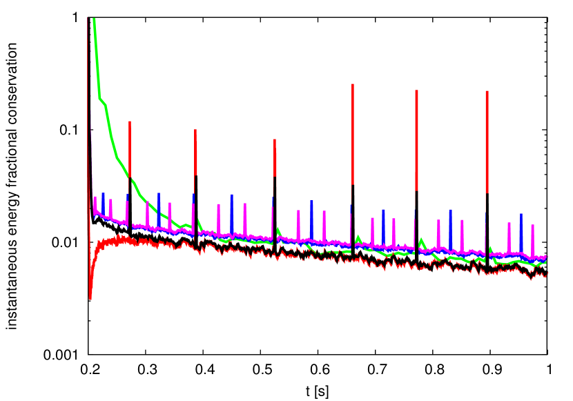
Figure B.2: Total energy $E_{\mathrm{total}}$ (normalized with the stellar initial energy) and instantaneous energy fractional conservation for a PNS with the CBF-EI EoS and $1.60\,\mathrm{M_{\odot}}$ baryon mass. The timestep dt is kept fixed during the evolution and n is the number of grid points. The plots begin at $200\,\mathrm{ms}$ because this is the initial time of our simulations (see Sec. 3.4).

The total energy and other quantum numbers (i.e., the baryon number) are conserved in every physical process. Our code enforces the conservation of the total baryon number $A=M_{\mathrm{B}}/m_{n}$, but as it evolves, the PNS loses energy and lepton number since neutrinos are allowed to escape from the star. Since the total energy of a star (matter plus neutrinos) in spherical symmetry is given by its gravitational mass $M$, the total energy of the system (stellar energy plus energy of the emitted neutrinos) is given by

$$E_{\mathrm{total}}=M(t)+\int_{200\,\mathrm{ms}}^{t}L_{\nu}(t)\mathrm{d}t,$$ (B.1)

where $L_{\nu}$ is defined in Eq. (3.141). Similarly, for the electron lepton number,

$$N_{\mathrm{total}}={} N_{L}(t)+\int_{200\,\mathrm{ms}}^{t}4\pi R^{2}\mathrm{e}^{\phi(R)}F_{\nu}(R)\mathrm{d}t,$$ (B.2)

$$N_{L}={} \int_{0}^{A}Y_{L}(a)\mathrm{d}a,$$ (B.3)

where $N_{L}$ is the total number of electronic leptons in the star, and $F_{\nu}$ is the electron neutrino number flux (we do not account for the other lepton numbers since we do not include muons and tauons in the EoSs and moreover $\mu_{\nu_{\mu}}=\mu_{\nu_{\tau}}=0$).

Since the conservation of $E_{\mathrm{total}}$ and $N_{\mathrm{total}}$ has not been enforced, they provide a test for our simulations. From Fig. B.1 and from the top plot of Fig. B.2, it is clear that they are conserved better than about $0.03\%$ during the evolution.

In Fig. B.2 we show, for different fixed timesteps and for different grid dimensions, the total and instantaneous energy fractional conservation from 0.2 s to 1 s. The instantaneous energy fractional conservation is defined as

$$\mathrm{i.e.f.c.}=\frac{|\dot{M}+L_{\nu}|}{L_{\nu}}.$$ (B.4)

We see that reducing the timestep the energy conservation is improved. The instantaneous energy fractional conservation as a function of time shows regular spikes, whose number doubles (triples) if we double (triple) the grid points, and whose magnitude is approximately inversely proportional to the timestep. We explain these spikes with the non-linearity of the transport equations (Press et al., (1992), Sec. 19.1). In fact, the temperature and the neutrino degeneracy appear inside and outside the gradients in the transport equations [Eqs. (3.105)–(3.108)]. As a consequence, the power in the Fourier space is accumulated in the shorter wavelengths and is finally released in the longer wavelengths of the solution. This explains why the frequency of the peaks changes with the grid spacing. The spikes of the instantaneous energy conservation have magnitudes which increase when the timestep is lowered, since one is dividing over a smaller timestep an approximately constant energy jump, $[M(t+\mathrm{d}t)-M(t)]/\mathrm{d}t$. These spikes do not undermine the overall conservation of the energy and lepton number and the PNS evolution, see Fig. B.1 and upper plot of Fig. B.2.

B.2 Beta-equilibrium assumption

Our code (as Keil and Janka,, 1995) assumes beta-equilibrium, Eqs. (2.31). This approximation is valid if the timescale of the beta-equilibrium is shorter than the dynamical timescale. We estimate the beta-equilibrium timescale using Eqs. (16) and (17a) of Burrows and Lattimer, (1986),

$$t_{\mathrm{beta}}={} \frac{1}{D_{n}},$$ (B.5)

$$D_{n}={} 1.86\times 10^{-2}Y_{p}T^{5}[S_{4}(\eta_{e})-S_{4}(\eta_{\nu})]\frac{1-\mathrm{e}^{-\Delta/T}}{1-\mathrm{e}^{-\eta_{e}+\eta_{\nu}}}\mathrm{\frac{neutrinos}{baryon\cdot s}},$$ (B.6)

$$S_{4}(y)={} \frac{y^{5}}{5}+2\pi^{2}\frac{y^{3}}{3}+7\pi^{4}\frac{y}{15},$$ (B.7)

where $D_{n}$ is the net rate of production of electron-neutrinos, $\eta=\mu/T$ is the degeneracy parameter, and $\Delta=0$ in the case of beta-equilibrium (we refer the reader to Burrows and Lattimer,, 1986 for more details). Since we have assumed beta-equilibrium, we put $1-\exp(-\Delta/T)\equiv 1$ to estimate the corresponding timescale. This means that the value of the beta-equilibrium timescale is not fully consistent.

We estimate the dynamical timescale with the formula

$$t_{\mathrm{dyn}}=R\frac{n_{\nu}(r)}{F_{\nu}(r)},$$ (B.8)

where $n_{\nu}(r)$ and $F_{\nu}(r)$ are the neutrino number density and number flux, respectively (which depend on the radial coordinate $r$), and $R$ is the stellar radius (notice that $F_{\nu}/n_{\nu}$ has the dimension of a velocity).

In Fig. B.3 we plot the dynamical and beta-equilibrium timescales for a PNS with the CBF-EI EoS and $M_{\mathrm{B}}=1.60\,\mathrm{M_{\odot}}$. The beta-equilibrium is valid in most of the star, apart for a thin shell near the border. Towards the end of the evolution the dynamical timescale seems to reduce, and this is conterintuitive. In fact, we have associated the dynamical timescale with the neutrino timescale. This is not true towards the end of the evolution, since as the PNS becomes optically thin the neutrinos decouple from the matter and the diffusion approximation breaks down. At that point, the neutrino timescale drops, but the stellar dynamics is actually frozen.

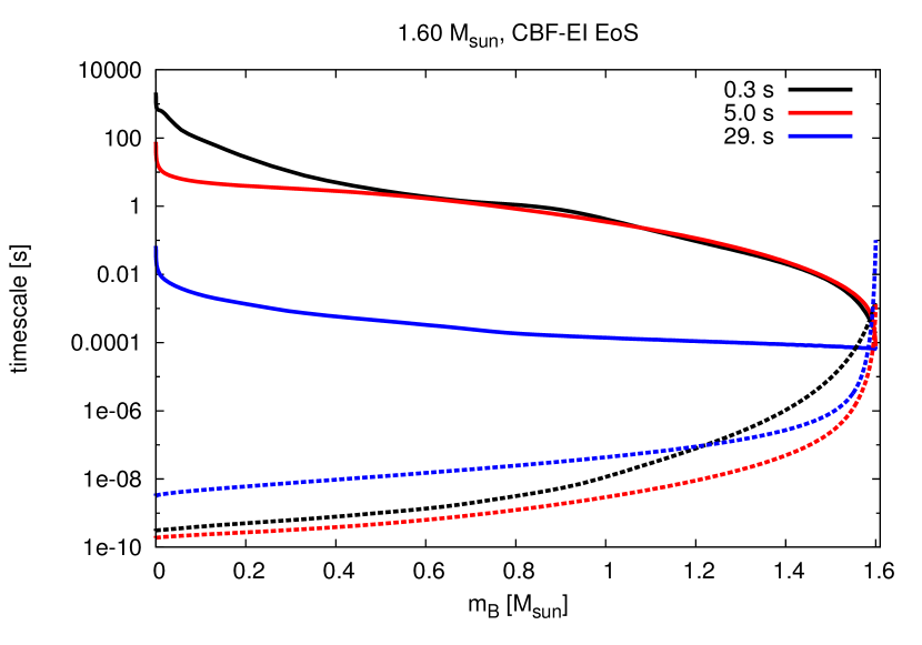
Figure B.3: Dynamical timescale (solid lines) and beta-equilibrium timescale (dashed lines) profiles at different times for a PNS with the CBF-EI EoS and $1.60\,\mathrm{M_{\odot}}$ stellar mass.

B.3 Interacting nucleon gas assumption

In this thesis we have not consider the formation of any kind of crust or envelope, that is, the EoS baryon part is made by an interacting gas of protons and neutrons. However, at low temperature and baryon density, the matter is not constitute only by a gas of baryons. The alpha particles (i.e., Helium nuclei) are the first species that appear decreasing the temperature and the density. The critical temperature at which alpha particles begin to form, that is, the lowest temperature at which protons and neutrons are present only as an interacting gas, depends on the baryon density and the proton fraction. Eq. (2.31) of Lattimer and Swesty, (1991) is an estimate of this critical temperature,

$$T_{c}(Y_{p})=87.76\left(\frac{K_{s}}{375\,\mathrm{MeV}}\right)^{1/2}\left(\frac{0.155\,\mathrm{fm^{-3}}}{n_{s}}\right)^{1/3}Y_{p}(1-Y_{p})\,\,\mathrm{MeV},$$ (B.9)

where $n_{s}$ and $K_{s}$ are the saturation density and the imcompressibility parameter at saturation density of symmetric nuclear matter (see Sec. 2.3). Eq. (B.9) is valid for $n_{\mathrm{B}}<n_{s}$, otherwise no alpha particles may form. In Fig. B.4 we report the profiles of the critical temperature and the PNS temperature for different snapshots of a PNS with the CBF-EI EoS and with $M_{\mathrm{B}}=1.60\,\mathrm{M_{\odot}}$; the results for the other EoSs and baryon masses are similar. As expected, the assumption of a proton-neutron interacting gas is valid at the beginning of the simulation and loses accuracy towards the end of the evolution, when it is not valid only in the outermost layers.

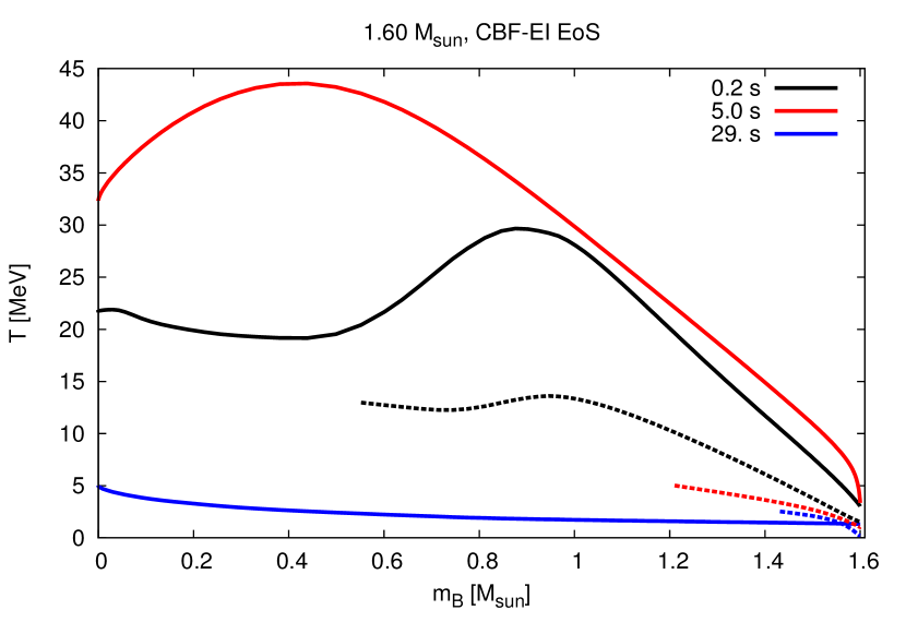
Figure B.4: Stellar temperature (solid lines) and critical temperature (dashed lines) for the formation of alpha particles at different times, for a PNS with the CBF-EI EoS and $1.60\,\mathrm{M_{\odot}}$ baryon mass. When the baryon density reaches the nuclei density, $0.155\,\mathrm{fm^{-3}}$, alpha particles could not form and we do not plot the critical temperature anymore.

Appendix C On the neutrino inverse reactions

The relevant nuclear processes in the neutrino diffusion during the PNS evolution are : the neutrino scattering on neutrons, protons, and electrons, the neutrino absorption on neutrons, the antineutrino absorption on protons, and their inverse processes. Such reactions are accounted in Eqs. (2.52)–(2.56). The Reactions (2.52)–(2.56) are accounted for in Reddy et al., (1998), in Pons et al., (1999), and in our work at the tree level, see Figs. C.1 and C.2. These processes are the neutrino scattering on neutrons, protons, and electrons, the neutrino absorption on neutrons, the antineutrino absorption on protons, and their inverse processes. In this appendix we explain how to account for the inverse process in the determination of the neutrino cross-section.

C.1 Direct reaction

In Fig. C.1 we show the Feynman diagram corresponding to the direct reaction, where one considers an incoming neutrino (particle 1) with a given energy $E_{1}$ that interacts with another incoming particle (particle 2). In the case of scattering, the outgoing particle 3 is a neutrino, instead in the case of absorption it is an electron or a positron.

feynman (3,3)(3,3) (250,100) i1,i2 o1,o2 1i1 3i2 2o1 4o2 fermioni1,v1 fermion,label=$1-f_{3}(E_{3})$,label.side=leftv1,i2 fermion,label=$f_{2}(E_{2})$,label.side=righto1,v2 fermion,label=$1-f_{4}(E_{4})$,label.side=rightv2,o2 photon,label=$q_{\mu}$,label.side=rightv1,v2 the end.Ωend.Ωendinput;

Figure C.1: Feynman diagram of the direct reaction: the incoming particles are 1 and 2, the outgoing particles are 3 and 4. In the computation of the direct cross section [Eq. (C.1)], one has to account for the distribution function of particle 2 and the Pauli-blocking effect for particles 3 and 4.

To determine the neutrino cross-section $\sigma_{j}^{\nu_{i}}(\omega)\equiv\sigma(E_{1})$ in Eq. (2.51) for the direct reactions, that is, the cross-section of a neutrino $\nu_{i}$ with energy $\omega\equiv E_{1}$ in the direct reaction $j$, we make use of Eq. (82) of Reddy et al., (1998),

$$\frac{\sigma(E_{1})}{V}={} \frac{G_{F}^{2}}{2\pi^{2}E_{1}^{2}}\int_{-\infty}^{E_{1}}\mathrm{d}q_{0}\frac{1-f_{3}(E_{3})}{1-\exp\left[\frac{-q_{0}-(\mu_{2}-\mu_{4})}{T}\right]}$$

$$\times\int_{|q_{0}|}^{E_{1}+E_{3}}\mathrm{d}qqq_{\mu}^{2}[AR_{1}+R_{2}+BR_{3}].$$ (C.1)

As in Reddy et al., (1998), we have set $c=h=1$, $G_{F}$ is the Fermi weak coupling constant, $f_{i}(E_{i})$ is the distribution function of the particle $i$ with energy $E_{i}$ and chemical potential $\mu_{i}$, $q^{\mu}=p_{1}^{\mu}-p_{3}^{\mu}$ is the transferred four-momentum, $A=(4E_{1}E_{3}+q_{\mu}^{2})/(2q^{2})$, $B=E_{1}+E_{3}$, and $R_{1}$, $R_{2}$, and $R_{3}$ are the response functions (Reddy et al.,, 1998). The integration limits for $q_{0}$, namely $-\infty$ and $E_{1}$, are due to the fact that $q_{0}=E_{1}-E_{3}$ and $E_{3}>0$. The integration limits for $q$ can be obtained from $q^{2}=E_{1}^{2}+E_{3}^{2}-2E_{1}E_{3}\cos\theta_{13}$, where $\theta_{13}$ is the angle between $\mathbf{p}_{1}$ and $\mathbf{p}_{3}$. We write the upper limit of the integration of $q$ as $E_{1}+E_{3}$ instead of as $2E_{1}-q_{0}$ as in Reddy et al., (1998), because this will simplify the discussion of the inverse reaction. It is useful to rewrite Eq. (C.1) as

$$\frac{\sigma^{\mathrm{d}}(E_{1})}{V}={} \int_{-\infty}^{E_{1}}\mathrm{d}q_{0}\big{[}1-f_{3}(E_{3})\big{]}\tilde{W}(q_{0},2,4),$$ (C.2)

$$\tilde{W}(q_{0},2,4)={} \frac{G_{F}^{2}}{2\pi^{2}E_{1}^{2}}\left(1-\exp\left[\frac{-q_{0}-(\mu_{2}-\mu_{4})}{T}\right]\right)$$

$$\times\int_{|q_{0}|}^{E_{1}+E_{3}}\mathrm{d}qqq_{\mu}^{2}[AR_{1}+R_{2}+BR_{3}],$$ (C.3)

where the superscript “d” means that it is the cross-section of the direct reaction and we put a tilde in the conveniently defined function $\tilde{W}$ because it is not a transition rate, and it depends on the properties of particles 2 and 4 (their masses, chemical potentials, and effective spectra, see Reddy et al.,, 1998).

C.2 Inverse reaction

Eq. (C.2) describes the direct process, that is, it is the cross section of an incoming neutrino with energy $E_{1}$. However, in Eq. (2.51) one needs to account also for the inverse process, namely one should include also the cross section of an outgoing neutrino with energy $E_{1}$, represented in Fig. C.2. In the inverse reaction the outgoing neutrino (particle 1) with a given energy $E_{1}$ is the result of the interaction of the incoming particles 3 and 4. In the case of inverse scattering, the incoming particle 3 is a neutrino, instead in the case of emission it is an electron or a positron.

feynman2 (3,3)(3,3) (250,100) i1,i2 o1,o2 1i1 3i2 2o1 4o2 fermionv1,i1 fermion,label=$f_{3}(E_{3})$,label.side=lefti2,v1 fermion,label=$1-f_{2}(E_{2})$,label.side=rightv2,o1 fermion,label=$f_{4}(E_{4})$,label.side=righto2,v2 photon,label=$q_{\mu}$,label.side=rightv2,v1 the end.Ωend.Ωendinput;

Figure C.2: Feynman diagram of the inverse reaction: the incoming particles are 3 and 4, the outgoing particles are 1 and 2. In the computation of the inverse cross section, one has to account for the distribution function of particles 3 and 4 and the Pauli-blocking effect for particle 2.

The direct Feynman diagram in Fig. C.1 is formally identical to the inverse one in Fig. C.2, provided that the following substitutions are made

• $2\leftrightarrow 4$;

• $1-f_{3}(E_{3})\rightarrow f_{3}(E_{3})$;

• $q_{\mu}\rightarrow-q_{\mu}$.

This correspond to the following expression for the inverse reaction (cf. Eq. (2.13) of Iwamoto and Pethick,, 1982):

$$\frac{\sigma^{\mathrm{i}}(E_{1})}{V}=\int_{-\infty}^{E_{1}}\mathrm{d}q_{0}f_{3}(E_{3})\tilde{W}(-q_{0},4,2),$$ (C.4)

where the superscript “i” denotes the cross-section of the inverse process and $\tilde{W}$ is defined as in Eq. (C.1). In Eq. (C.4) the transferred momentum is $q^{\mu}=p^{\mu}_{3}-p^{\mu}_{1}$, and therefore the boundaries of the integrals in $q_{0}$ and $q$ are the same as in Eq. (C.2). This would have not been the case if we had written the upper limit of the integration in $q$ as $2E_{1}-q_{0}$ (as in Reddy et al.,, 1998) instead of as $E_{1}+E_{3}$.

Eq. (C.4) has to be solved for the neutrino and antineutrino emission (i.e., the inverse reactions of the neutrino and antineutrino absorption), but in the case of the inverse scattering, where particles $2\equiv 4$ and $1\equiv 3$, one can use a simplified expression. In fact, the principle of detailed balance assures that in a systems invariant under spatial reflections, the following relation holds for the transition rate $W_{fi}$ (Iwamoto and Pethick,, 1982)

$$W_{fi}(\mathbf{q},q_{0})=\mathrm{e}^{\frac{q_{0}}{T}}W_{fi}(\mathbf{q},-q_{0}),$$ (C.5)

from which one has, since $\mu_{1}\equiv\mu_{3}$,

$$\tilde{W}(-q_{0},4,2)={} \mathrm{e}^{\frac{(E_{3}-\mu_{3})-(E_{1}-\mu_{1})}{T}}\tilde{W}(q_{0},2,4),$$ (C.6)

$$\frac{\sigma^{\mathrm{s,i}}}{V}={} -\mathrm{e}^{-\frac{E_{1}-\mu_{1}}{T}}\frac{\sigma^{\mathrm{s,d}}}{V},$$ (C.7)

and, finally,

$$\frac{\sigma^{\mathrm{s,tot}}(E_{1})}{V}=\frac{\sigma^{\mathrm{s,i}}(E_{1})}{V}+\frac{\sigma^{\mathrm{s,d}}(E_{1})}{V}=\frac{1}{1-f_{1}(E_{1})}\times\frac{\sigma^{\mathrm{s,d}}(E_{1})}{V},$$ (C.8)

where the superscript “s” implies that we are only considering the scattering reactions.

References

- Abbot et al., (2016) Abbot, B. P. et al. (2016). Observation of gravitational waves from a binary black hole merger. PRL, 116:061102.
- Alekseev et al., (1987) Alekseev, E. N., Alekseeva, L. N., Volchenko, V. I., and Krivosheina, I. V. (1987). Possible detection of a neutrino signal on 23 February 1987 at the Baksan underground scintillation telescope of the Institute of Nuclear Research. Soviet Journal of Experimental and Theoretical Physics Letters, 45:589.
- Andersson et al., (2011) Andersson, N., Ferrari, V., Jones, D. I., Kokkotas, K. D., Krishnan, B., Read, J. S., Rezzolla, L., and Zink, B. (2011). Gravitational waves from neutron stars: promises and challenges. General Relativity and Gravitation, 43:409–436.
- (4) Andersson, N. and Kokkotas, K. D. (1998a). Pulsation modes for increasingly relativistic polytropes. MNRAS, 297:493–496.
- (5) Andersson, N. and Kokkotas, K. D. (1998b). Towards gravitational wave asteroseismology. MNRAS, 299:1059–1068.
- Andresen et al., (2016) Andresen, H., Mueller, B., Mueller, E., and Janka, H.-T. (2016). Gravitational Wave Signals from 3D Neutrino Hydrodynamics Simulations of Core-Collapse Supernovae. ArXiv e-prints.
- Andresen et al., (2017) Andresen, H., Müller, B., Müller, E., and Janka, H.-T. (2017). Gravitational Wave Signals from 3D Neutrino Hydrodynamics Simulations of Core-Collapse Supernovae. Mon. Not. Roy. Astron. Soc., 468(2):2032–2051.
- Benhar et al., (2004) Benhar, O., Ferrari, V., and Gualtieri, L. (2004). Gravitational wave asteroseismology reexamined. PRD, 70(12):124015.
- Benhar et al., (2005) Benhar, O., Ferrari, V., Gualtieri, L., and Marassi, S. (2005). Perturbative approach to the structure of rapidly rotating neutron stars. Phys. Rev., D72:044028.
- Benhar and Lovato, (2017) Benhar, O. and Lovato, A. (2017). Perturbation theory of nuclear matter with a microscopic effective interaction. PRC, 96(5):054301.
- Bethe and Wilson, (1985) Bethe, H. A. and Wilson, J. R. (1985). Revival of a stalled supernova shock by neutrino heating. ApJ, 295:14–23.
- Bionta et al., (1987) Bionta, R. M., Blewitt, G., Bratton, C. B., Casper, D., and Ciocio, A. (1987). Observation of a neutrino burst in coincidence with supernova 1987A in the Large Magellanic Cloud. Physical Review Letters, 58:1494–1496.
- Bombaci and Lombardo, (1991) Bombaci, I. and Lombardo, U. (1991). Asymmetric nuclear matter equation of state. Phys.Rev.C, 44:1892–1900.
- Bonazzola and Gourgoulhon, (1996) Bonazzola, S. and Gourgoulhon, E. (1996). Gravitational waves from pulsars: Emission by the magnetic field induced distortion. Astron. Astrophys., 312:675.
- Burgio et al., (2011) Burgio, G. F., Ferrari, V., Gualtieri, L., and Schulze, H.-J. (2011). Oscillations of hot, young neutron stars: Gravitational wave frequencies and damping times. PRD, 84(4):044017.
- Burgio and Schulze, (2010) Burgio, G. F. and Schulze, H.-J. (2010). The maximum and minimum mass of protoneutron stars in the Brueckner theory. A&A, 518:A17.
- Burrows, (1988) Burrows, A. (1988). Supernova neutrinos. ApJ, 334:891–908.
- Burrows and Lattimer, (1986) Burrows, A. and Lattimer, J. M. (1986). The birth of neutron stars. ApJ, 307:178–196.
- Camelio et al., (2016) Camelio, G., Gualtieri, L., Pons, J. A., and Ferrari, V. (2016). Spin evolution of a proto-neutron star. PRD, 94(2):024008.
- Camelio et al., (2017) Camelio, G., Lovato, A., Gualtieri, L., Benhar, O., Pons, J. A., and Ferrari, V. (2017). Evolution of a proto-neutron star with a nuclear many-body equation of state: Neutrino luminosity and gravitational wave frequencies. PRD, 96(4):043015.
- Chandrasekhar and Ferrari, (1990) Chandrasekhar, S. and Ferrari, V. (1990). The flux integral for axisymmetric perturbations of static space-times. Proceedings of the Royal Society of London Series A, 428:325–349.
- Christy, (1966) Christy, R. F. (1966). Pulsation Theory. Ann.Rev.A&A, 4:353.
- Ciolfi et al., (2010) Ciolfi, R., Ferrari, V., and Gualtieri, L. (2010). Structure and deformations of strongly magnetized neutron stars with twisted torus configurations. Mon. Not. Roy. Astron. Soc., 406:2540–2548.
- Clark, (1979) Clark, J. W. (1979). Variational theory of nuclear matter. Progress in Particle and Nuclear Physics, 2:89 – 199.
- Couch and Ott, (2015) Couch, S. M. and Ott, C. D. (2015). The Role of Turbulence in Neutrino-Driven Core-Collapse Supernova Explosions. Astrophys. J., 799(1):5.
- Cowling, (1941) Cowling, T. G. (1941). The non-radial oscillations of polytropic stars. MNRAS, 101:367.
- Cox and Giuli, (1968) Cox, J. P. and Giuli, R. T. (1968). Principles of stellar structure .
- Detweiler and Lindblom, (1985) Detweiler, S. and Lindblom, L. (1985). On the nonradial pulsations of general relativistic stellar models. ApJ, 292:12–15.
- Dimmelmeier et al., (2002) Dimmelmeier, H., Font, J. A., and Müller, E. (2002). Relativistic simulations of rotational core collapse II. Collapse dynamics and gravitational radiation. A&A, 393:523–542.
- Doneva et al., (2013) Doneva, D. D., Gaertig, E., Kokkotas, K. D., and Krüger, C. (2013). Gravitational wave asteroseismology of fast rotating neutron stars with realistic equations of state. Phys. Rev., D88(4):044052.
- Duff, (2015) Duff, M. J. (2015). How fundamental are fundamental constants? Contemporary Physics, 56:35–47.
- Duff et al., (2002) Duff, M. J., Okun, L. B., and Veneziano, G. (2002). Trialogue on the number of fundamental constants. Journal of High Energy Physics, 3:023.
- Dvornikov and Dib, (2010) Dvornikov, M. and Dib, C. (2010). Spin-down of neutron stars by neutrino emission. Phys. Rev., D82:043006.
- Eggleton et al., (1973) Eggleton, P. P., Faulkner, J., and Flannery, B. P. (1973). An Approximate Equation of State for Stellar Material. A&A, 23:325.
- Epstein, (1978) Epstein, R. (1978). Neutrino angular momentum loss in rotating stars. ApJL, 219:L39–L41.
- Fantoni and Rosati, (1974) Fantoni, S. and Rosati, S. (1974). Jastrow correlations and an irreducible cluster expansion for infinite boson or fermion systems. Nuovo Cim., A20:179–193.
- Ferrari et al., (2003) Ferrari, V., Miniutti, G., and Pons, J. A. (2003). Gravitational waves from newly born, hot neutron stars. MNRAS, 342:629–638.
- Fick, (1855) Fick, A. (1855). Ueber Diffusion. Annalen der Physik, 170:59–86.
- Fick, (1995) Fick, A. (1995). On liquid diffusion. Journal of Membrane Science, 100:33–38.
- Fischer, (2016) Fischer, T. (2016). The role of medium modifications for neutrino-pair processes from nucleon-nucleon bremsstrahlung. Impact on the protoneutron star deleptonization. A&A, 593:A103.
- Fischer et al., (2010) Fischer, T., Whitehouse, S. C., Mezzacappa, A., Thielemann, F.-K., and Liebendörfer, M. (2010). Protoneutron star evolution and the neutrino-driven wind in general relativistic neutrino radiation hydrodynamics simulations. A&A, 517:A80.
- Fujita and Miyazawa, (1957) Fujita, J. and Miyazawa, H. (1957). Pion Theory of Three-Body Forces. Progress of Theoretical Physics, 17:360–365.
- Fuller et al., (2015) Fuller, J., Klion, H., Abdikamalov, E., and Ott, C. D. (2015). Supernova Seismology: Gravitational Wave Signatures of Rapidly Rotating Core Collapse. Mon. Not. Roy. Astron. Soc., 450(1):414–427.
- Glendenning, (1985) Glendenning, N. K. (1985). Neutron stars are giant hypernuclei? ApJ, 293:470–493.
- Glendenning and Moszkowski, (1991) Glendenning, N. K. and Moszkowski, S. A. (1991). Reconciliation of neutron-star masses and binding of the Lambda in hypernuclei. Physical Review Letters, 67:2414–1417.
- Gourgoulhon et al., (1999) Gourgoulhon, E., Haensel, P., Livine, R., Paluch, E., Bonazzola, S., and Marck, J. A. (1999). Fast rotation of strange stars. Astron. Astrophys., 349:851.
- Goussard et al., (1997) Goussard, J.-O., Haensel, P., and Zdunik, J. L. (1997). Rapid uniform rotation of protoneutron stars. Astron. Astrophys., 321:822–834.
- Goussard et al., (1998) Goussard, J. O., Haensel, P., and Zdunik, J. L. (1998). Rapid differential rotation of protoneutron stars and constraints on radio pulsars periods. Astron. Astrophys., 330:1005–1016.
- Hanke et al., (2013) Hanke, F., Mueller, B., Wongwathanarat, A., Marek, A., and Janka, H.-T. (2013). SASI Activity in Three-Dimensional Neutrino-Hydrodynamics Simulations of Supernova Cores. Astrophys. J., 770:66.
- Hartle, (1967) Hartle, J. B. (1967). Slowly rotating relativistic stars. 1. Equations of structure. Astrophys. J., 150:1005–1029.
- Hartle, (1973) Hartle, J. B. (1973). Slowly rotating relativistic stars. Astrophysics and Space Science, 24(2):385–405.
- Hartle and Thorne, (1968) Hartle, J. B. and Thorne, K. S. (1968). Slowly Rotating Relativistic Stars. II. Models for Neutron Stars and Supermassive Stars. Astrophys. J., 153:807.
- Haskell et al., (2006) Haskell, B., Jones, D. I., and Andersson, N. (2006). Mountains on Neutron Stars: Accreted vs. Non-Accreted crusts. Mon. Not. Roy. Astron. Soc., 373:1423–1439.
- Heger et al., (2005) Heger, A., Woosley, S. E., and Spruit, H. C. (2005). Presupernova evolution of differentially rotating massive stars including magnetic fields. Astrophys. J., 626:350–363.
- Henriksen and Chau, (1978) Henriksen, R. N. and Chau, W. Y. (1978). Neutrino angular momentum loss by the Poynting-Robertson effect. ApJ, 225:712–718.
- Hirata et al., (1987) Hirata, K., Kajita, T., Koshiba, M., Nakahata, M., and Oyama, Y. (1987). Observation of a neutrino burst from the supernova SN1987A. Physical Review Letters, 58:1490–1493.
- Horowitz and Kadau, (2009) Horowitz, C. J. and Kadau, K. (2009). The Breaking Strain of Neutron Star Crust and Gravitational Waves. Phys. Rev. Lett., 102:191102.
- Hosaka et al., (2006) Hosaka, J. et al. (2006). Solar neutrino measurements in Super-Kamiokande-I. Phys.Rev.D, 73(11):112001.
- (59) Hüdepohl, L., Müller, B., Janka, H.-T., Marek, A., and Raffelt, G. G. (2010a). Erratum: Neutrino Signal of Electron-Capture Supernovae from Core Collapse to Cooling [Phys. Rev. Lett. 104, 251101 (2010)]. Physical Review Letters, 105(24):249901.
- (60) Hüdepohl, L., Müller, B., Janka, H.-T., Marek, A., and Raffelt, G. G. (2010b). Neutrino Signal of Electron-Capture Supernovae from Core Collapse to Cooling. Physical Review Letters, 104(25):251101.
- Ikeda et al., (2007) Ikeda, M. et al. (2007). Search for Supernova Neutrino Bursts at Super-Kamiokande. ApJ, 669:519–524.
- Iwamoto and Pethick, (1982) Iwamoto, N. and Pethick, C. J. (1982). Effects of nucleon-nucleon interactions on scattering of neutrinos in neutron matter. PRD, 25:313–329.
- Janka, (2004) Janka, H.-T. (2004). Neutron star formation and birth properties. [IAU Symp.218,3(2004)].
- Janka and Mönchmeyer, (1989) Janka, H.-T. and Mönchmeyer, R. (1989). Hydrostatic post bounce configurations of collapsed rotating iron cores-neutrino emission. Astronomy and Astrophysics, 226:69–87.
- Johns et al., (1996) Johns, S. M., Ellis, P. J., and Lattimer, J. M. (1996). Numerical Approximation to the Thermodynamic Integrals. ApJ, 473:1020.
- Johnson-McDaniel and Owen, (2013) Johnson-McDaniel, N. K. and Owen, B. J. (2013). Maximum elastic deformations of relativistic stars. Phys. Rev., D88:044004.
- Jones, (2002) Jones, D. I. (2002). Gravitational waves from rotating neutron stars. Class. Quant. Grav., 19:1255–1266.
- Jones and Andersson, (2001) Jones, D. I. and Andersson, N. (2001). Freely precessing neutron stars: model and observations. Mon. Not. Roy. Astron. Soc., 324:811.
- Kazanas, (1977) Kazanas, D. (1977). Neutrino angular momentum losses in stellar collapse. Nature, 267:501.
- Keil and Janka, (1995) Keil, W. and Janka, H.-T. (1995). Hadronic phase transitions at supranuclear densities and the delayed collapse of newly formed neutron stars. A&A, 296:145.
- Kotake, (2013) Kotake, K. (2013). Multiple physical elements to determine the gravitational-wave signatures of core-collapse supernovae. Comptes Rendus Physique, 14:318–351.
- Krane, (1987) Krane, K. S. (1987). Introductory Nuclear Physics.
- Kunkel et al., (1987) Kunkel, W., Madore, B., Shelton, I., Duhalde, O., Bateson, F. M., Jones, A., Moreno, B., Walker, S., Garradd, G., Warner, B., and Menzies, J. (1987). Supernova 1987A in the Large Magellanic Cloud. IAU Circ., No., 4316.
- Kuroda et al., (2016) Kuroda, T., Kotake, K., and Takiwaki, T. (2016). A new Gravitational-wave Signature From Standing Accretion Shock Instability in Supernovae. Astrophys. J., 829(1):L14.
- Lattimer and Prakash, (2001) Lattimer, J. M. and Prakash, M. (2001). Neutron star structure and the equation of state. Astrophys. J., 550:426.