On the application of the Lindstedt-Poincaré method to the Lotka-Volterra system

Abstract

We apply the Lindstedt-Poincaré method to the Lotka-Volterra model and discuss alternative implementations of the approach. By means of an efficient systematic algorithm we obtain an unprecedented number of perturbation corrections for the two dynamical variables and the frequency. They enable us to estimate the radius of convergence of the perturbation series for the frequency as a function of the only model parameter. The method is suitable for the treatment of systems with any number of dynamical variables.

1 Introduction

In the last three decades there has been some interest in the application of perturbation theory to nonlinear dynamical systems such as the Lotka-Volterra model. Murty et al[1] applied perturbation theory to a three-species ecological system and obtained the first perturbation correction to the population of each species. However, they did not take into account that the secular terms spoil the approximate result that will not exhibit the expected periodic behaviour. Grozdanovski and Shepherd[2] applied the well-known Lindstedt-Poincaré method to remove secular terms and obtained the first two perturbation corrections to a two-species system. Consequently, their approximate results exhibit the expected periodic behaviour. Navarro[3] also applied the Lindstedt-Poincaré method to the same two-species system and obtained periodic approximate expressions of second order. This author proposed a symbolic algorithm for the computation of periodic orbits but surprisingly did not show results of larger order. Navarro and Poveda[4] applied Navarro’s approach to a three-species system and derived perturbation corrections of first and second order for the populations of the three species for some particular values of the model parameters. All these studies lead to the conclusion that the Lindstedt-Poincaré method gives reasonable results for some model parameters and suggest that the technique may be useful for the analysis of more realistic and related nonlinear dynamical problems.

Unfortunately Grozdanovski and Shepherd[2] did not explicitly indicate the initial conditions chosen for the solution of the first-order differential equations that provide the corrections at every perturbation order. Since their strategy is not clearly delineated it is difficult to derive a systematic approach for the calculation of perturbation corrections of greater order. On the other hand, Navarro[3] and Navarro and Poveda[4] put forward a systematic symbolic algorithm but they did not appear to exploit it to obtain perturbation corrections of large order. Besides, their presentation of the algorithm appears to be rather obscure for anybody who is not familiar with such technique.

The aim of this paper is the analysis of the approach proposed by Grozdanovski and Shepherd[2] with the purpose of deriving a systematic method for the calculation of perturbation corrections of any order to the Lotka-Volterra model. Such results may give us some clue about the convergence properties of the perturbation series. In addition to it we investigate the possibility of generalizing the method for the treatment of more realistic systems with more than two degrees of freedom.

In section 2 we outline the Lotka-Volterra model and compare alternative implementations of the Lindstedt-Poincaré approach. In section 3 we put forward a generalization of the method that enables one to treat all the previously discussed cases. In section 4 we carry out a large order calculation of the perturbation corrections and estimate the radius of convergence of the perturbation series for the frequency. Finally, in section 5 we outline the application of the method to more general and realistic dynamical systems and draw conclusions.

2 The Lindstedt-Poincaré method

In this section we briefly discuss the Lotka-Volterra model and delineate the application of the Lindsted-Poincaré technique. For concreteness we will follow Grozdanovski and Shepherd[2] because their treatment of the dynamical equations is clear and straightforward.

2.1 The model

The dynamical equations for the model are

$$\dot{X}(T)=X(T)\left[a-bY(T)\right],\;\dot{Y}(T)=Y(T)\left[cX(T)-d\right],$$ (1)

where $a$, $b$, $c$ and $d$ are positive parameters and the point indicates derivative with respect to time. The physical meaning of the parameters is not relevant for present purposes because we are mainly interested in the success of the perturbation approach. Besides, most probably nobody will apply the Lotka-Volterra model to an actual ecological system today because it is quite unrealistic. The interested reader may resort to the papers cited above for more information[1, 2, 3, 4] (and the references cited therein).

We can get rid of some model parameters by means of the following transformations of the independent and dependent variables

$$t=aT,\;x(t)=\frac{c}{d}X(T),\;y(t)=\frac{b}{a}Y(T).$$ (2)

The resulting equations

$$\dot{x}(t)=x(t)-x(t)y(t),\;\dot{y}(t)=\alpha\left[-y(t)+x(t)y(t)\right],$$ (3)

depend on just one parameter $\alpha=d/a$.

There is a stationary point at $x=1$ and $y=1$. Therefore, if we define

$$x(t)=1+\epsilon\xi(t),\;y(t)=1+\epsilon\eta(t),$$ (4)

the resulting dynamical equations will depend on the perturbation parameter $\epsilon$

$$\dot{\xi}(t)=-\eta(t)-\epsilon\xi(t)\eta(t),\;\dot{\eta}(t)=\alpha\left[\xi(t)+\epsilon\xi(t)\eta(t)\right].$$ (5)

In order to apply the Lindstedt-Poincaré method we define the dimensionless time

$$\tau=\omega t,$$ (6)

where $\omega$ is the unknown frequency of oscillation. In this way we have

$$\omega\dot{\xi}(\tau)=-\eta(\tau)-\epsilon\xi(\tau)\eta(\tau),\;\omega\dot{\eta}(\tau)=\alpha\left[\xi(\tau)+\epsilon\xi(\tau)\eta(\tau)\right].$$ (7)

Following Grozdanovski and Shepherd[2] we are using the same symbols $\xi$ and $\eta$ for the solutions of equations (5) and (7). Besides, we have chosen a dot to indicate the derivative with respect to either $t$ or $\tau$. Although this practice may be unwise when one is studying a practical problem and wants to reconstruct $X(T)$ and $Y(T)$ from $\xi(\tau)$ and $\eta(\tau)$ it is harmless in the present case because our aim is to show how to obtain perturbation corrections of large order and study the convergence of the perturbation series.

2.2 Perturbation equations

We now assume that $\epsilon$ is a sufficiently small parameter and apply perturbation theory in the usual way

$$\xi(\tau) = \sum_{j=0}^{\infty}\xi_{j}(\tau)\epsilon^{j},$$

$$\eta(\tau) = \sum_{j=0}^{\infty}\eta_{j}(\tau)\epsilon^{j},$$

$$\omega = \sum_{j=0}^{\infty}\omega_{j}\epsilon^{j}.$$ (8)

From the equations of order zero ($\epsilon=0$) we obtain

$$\xi_{0}(\tau)=A\cos(\tau+\phi),\,\eta_{0}(\tau)=\sqrt{\alpha}A\sin(\tau+\phi),$$ (9)

and $\omega_{0}=\sqrt{\alpha}$. On inserting the expansions (8) into equations (7) it is not difficult to show that the perturbation corrections are solutions to

$$\dot{\xi}_{n} = -\frac{1}{\sqrt{\alpha}}\eta_{n}+F_{n},\;n=1,2,\ldots,$$

$$\dot{\eta}_{n} = \sqrt{\alpha}\xi_{n}+G_{n}$$

$$F_{n} = -\frac{1}{\sqrt{\alpha}}\sum_{j=0}^{n-1}\xi_{j}\eta_{n-j-1}-\frac{1}{\sqrt{\alpha}}\sum_{j=1}^{n}\omega_{j}\dot{\xi}_{n-j},$$

$$G_{n} = \sqrt{\alpha}\sum_{j=0}^{n-1}\xi_{j}\eta_{n-j-1}-\frac{1}{\sqrt{\alpha}}\sum_{j=1}^{n}\omega_{j}\dot{\eta}_{n-j}.$$ (10)

2.3 Systematic approach

The purpose of this subsection is to derive general expressions for the solutions to the perturbation equations (10) that enable us to develop a systematic algorithm for the calculation of corrections of sufficiently large order.

Neither Grozdanovski and Shepherd[2] nor Navarro[3] consider the initial conditions of the perturbation corrections $\xi_{n}(\tau)$ and $\eta_{n}(\tau)$ explicitly. Here we choose

$$\xi_{n}(0)=0,\;\eta_{n}(0)=0,\;n>0,$$ (11)

because they greatly facilitate the calculation of $A$ and $\phi$ from $x(0)$ and $y(0)$:

$$x(0)=1+\epsilon A\cos(\phi),\;y(0)=1+\epsilon A\sqrt{\alpha}\sin(\phi).$$ (12)

Note that, given $x(0)$ and $y(0)$ we obtain the product $\epsilon A$ and $\phi$. Later on we will show why $A$ always appears associated to the perturbation parameter $\epsilon$ in this particular way.

In order to solve equations (10) we rewrite them in matrix form

$$\mathbf{\dot{W}}_{n} = \mathbf{K\cdot W}_{n}+\mathbf{R}_{n},$$

$$\mathbf{W}_{n} = \left(\begin{array}[]{l}\xi_{n}\\ \eta_{n}\end{array}\right),\;\mathbf{R}_{n}=\left(\begin{array}[]{l}F_{n}\\ G_{n}\end{array}\right),$$ (17)

$$\mathbf{K} = \frac{1}{\sqrt{\alpha}}\left(\begin{array}[]{ll}0&-1\\ \alpha&0\end{array}\right),$$ (20)

so that the solution is simply given by

$$\mathbf{W}_{n}(\tau)=\int_{0}^{\tau}\exp\left[(\tau-s)\mathbf{K}\right]\cdot\mathbf{R}_{n}(s)\mathbf{\,}ds,$$ (21)

where

$$\exp\left(\tau\mathbf{K}\right)=\frac{1}{\sqrt{\alpha}}\left(\begin{array}[]{ll}\sqrt{\alpha}\cos(\tau)&-\sin(\tau)\\ \alpha\sin(\tau)&\sqrt{\alpha}\cos(\tau)\end{array}\right).$$ (22)

Note that equation (21) is consistent with the initial conditions (11).

In order to identify the resonant terms that would give rise to secular terms we rewrite the first-order differential equations as second order ones; for example

$$\ddot{\xi}_{n}=-\xi_{n}+\dot{F}_{n}-\frac{1}{\sqrt{\alpha}}G_{n}.$$ (23)

Therefore, we set $\omega_{n}$ so that

$$\int_{0}^{2\pi}\left[\dot{F}_{n}(\tau)-\frac{1}{\sqrt{\alpha}}G_{n}(\tau)\right]\sin(\tau+\phi)\,d\tau = 0,\,$$

$$\int_{0}^{2\pi}\left[\dot{F}_{n}(\tau)-\frac{1}{\sqrt{\alpha}}G_{n}(\tau)\right]\cos(\tau+\phi)\,d\tau = 0.$$ (24)

These equations are a generalization of the Lemma 1 in the paper by Grozdanovski and Shepherd[2] and the proposal of Navarro[3]. It is worth noting that the same value of $\omega_{n}$ satisfies both equations (24). We are not aware of a rigorous proof of this result but we can test it by means of our calculations of large order. This point was not discussed in the earlier papers on the application of the Lindstedt-Poincaré method to multidimensional systems[2, 3, 4] probably because they did not try to obtain a set of explicit equations for a systematic application of the approach.

Unfortunately, the perturbation corrections obtained in this way are considerably more complicated than those derived by Grozdanovski and Shepherd[2]. For example, at first order we obtain

$$\xi_{1}(\tau) = A^{2}\left[\frac{\sin{\left(\phi\right)}}{4}-\frac{\sqrt{\alpha}\cos{\left(3\phi\right)}}{12}-\frac{\sin{\left(3\phi\right)}}{12}-\frac{\sqrt{\alpha}\cos{\left(\phi\right)}}{4}\right]\sin(\tau+\phi)$$

$$+\frac{A^{2}\sqrt{\alpha}}{6}\sin[2(\tau+2\phi)]$$

$$+A^{2}\left[\frac{\sqrt{\alpha}\sin{\left(3\phi\right)}}{12}-\frac{\cos{\left(\phi\right)}}{4}-\frac{\cos{\left(3\phi\right)}}{12}-\frac{\sqrt{\alpha}\sin{\left(\phi\right)}}{4}\right]\cos(\tau+\phi)$$

$$+\frac{A^{2}}{3}\cos[2(\tau+\phi)],$$

$$\eta_{1}(\tau) = A^{2}\left[\frac{\alpha\sin{\left(3\phi\right)}}{12}-\frac{\sqrt{\alpha}\cos{\left(3\phi\right)}}{12}-\frac{\sqrt{\alpha}\cos{\left(\phi\right)}}{4}-\frac{\alpha\sin{\left(\phi\right)}}{4}\right]\sin(\tau+\phi)$$ (25)

$$+\frac{A^{2}\sqrt{\alpha}}{6}\sin[2(\tau+\phi)]$$

$$+A^{2}\left[\frac{\alpha\cos{\left(3\phi\right)}}{12}+\frac{\sqrt{\alpha}\sin{\left(3\phi\right)}}{12}+\frac{\alpha\cos{\left(\phi\right)}}{4}-\frac{\sqrt{\alpha}\sin{\left(\phi\right)}}{4}\right]\cos(\tau+\phi)$$

$$-\frac{A^{2}\alpha}{3}\cos[2(\tau+\phi)].$$

The coefficients of $\sin[2(\tau+2\phi)]$ and $\cos[2(\tau+2\phi)]$ agree with the ones derived earlier by those authors and the remaining terms are necessary to satisfy the initial conditions (11). We also find that $\omega_{1}=0$ removes the resonant terms. The perturbation corrections derived by Navarro[3] with somewhat different initial conditions appear to be simpler but they are restricted to $\alpha=1$.

The perturbation corrections of second order are so complicated that we do not show them here. Besides, $\omega_{3}$ is nonzero and a rather cumbersome function of $\alpha$ and $\phi$:

$$\omega_{3} = \frac{A^{3}\sqrt{\alpha}\left(\alpha+1\right)\cos{\left(3\phi\right)}}{144}-\frac{A^{3}\alpha\left(\alpha+1\right)\sin{\left(3\phi\right)}}{144}$$ (26)

$$+\frac{A^{3}\sqrt{\alpha}\left(\alpha+1\right)\cos{\left(\phi\right)}}{48}+\frac{A^{3}\alpha\left(\alpha+1\right)\sin{\left(\phi\right)}}{48}.$$

The occurrence of rather too complicated perturbation corrections appears to be the price that one has to pay for obtaining the simpler equations (12) for the calculation of $\epsilon A$ and $\phi$.

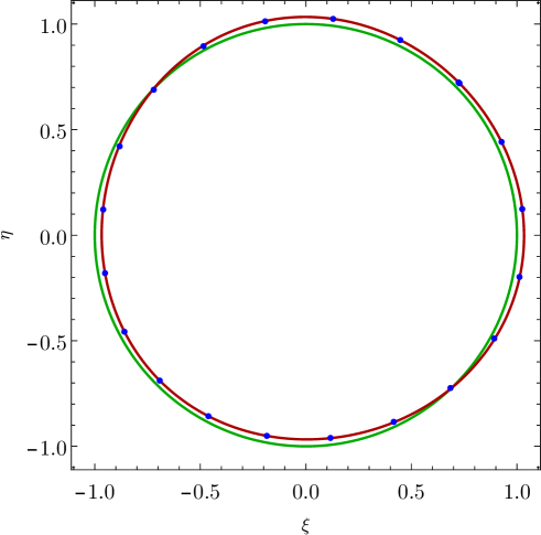
Figure 1: Curve $\eta(\xi)$ calculated by means of perturbation theory of order zero (dashed, green line), up to second order (continuous, red line) and numerically (blue points) for $\alpha=1$, $\epsilon A=0.1$ and $\phi=\pi/4$

At first sight the dependence of $\omega_{n}$ on the phase $\phi$ may appear to be the consequence of a wrong calculation. However, we have verified that present solutions already satisfy the perturbation equations and comparison with numerical results reveals a good agreement. For example, figure 1 compares the curve $\eta(\xi)$ for $\alpha=1$, $\epsilon A=0.1$ and $\phi=\pi/4$ calculated by perturbation theory of zeroth and second order and an accurate numerical result. We appreciate that the addition of the perturbation corrections shown above already improves the analytical results. In the next subsection we will explain the reason for the discrepancy between our expressions and those of Grozdanovski and Shepherd[2] in a more transparent way.

2.4 The straightforward Fourier expansion

The purpose of this subsection is merely to show why it is possible to obtain many different solutions at every order of perturbation theory. We may solve the differential perturbation equations (10) by inserting Fourier expansions of the form

$$\xi_{n}(\tau) = \sum_{j=1}^{n+1}a_{1j}^{(n)}\sin[j(\tau+\phi)]+\sum_{j=0}^{n+1}b_{1j}^{(n)}\cos[j(\tau+\phi)],$$

$$\eta_{n}(\tau) = \sum_{j=1}^{n+1}a_{2j}^{(n)}\sin[j(\tau+\phi)]+\sum_{j=0}^{n+1}b_{2j}^{(n)}\cos[j(\tau+\phi)].$$ (27)

For the first order we obtain (we omit the superscript for simplicity)

$$a_{11}+\frac{b_{21}}{\sqrt{\alpha}} = 0,\;b_{11}-\frac{a_{21}}{\sqrt{\alpha}}=0,$$

$$a_{12} = \frac{A^{2}\sqrt{\alpha}}{6},\;b_{12}=\frac{A^{2}}{3},\;a_{22}=\frac{A^{2}\sqrt{\alpha}}{6},\;b_{22}=-\frac{A^{2}\alpha}{3}.$$ (28)

We appreciate that if we choose $a_{11}=b_{21}=b_{11}=a_{21}=0$ we obtain exactly the results of Grozdanovski and Shepherd[2]. However, there is an infinite number of perfectly valid solutions that emerge from arbitrary choices of $a_{11}$, $b_{21}$, $b_{11}$ and $a_{21}$ provided that they satisfy the ratios $\frac{b_{21}}{a_{11}}=-\frac{a_{21}}{b_{11}}=-\sqrt{\alpha}$. One of such possible solutions is that shown above that satisfies the boundary conditions (11). The solutions derived by the authors just mentioned seem to be the simplest ones and are therefore most convenient for large-order calculations. We should find suitable general conditions to produce such simple results at every order of perturbation theory.

3 Generalization of the systematic approach

In the preceding sections we discussed two possible solutions: those that lead to the simple initial conditions (12) and those that are considerably simpler but lead to somewhat complicated initial conditions. The problem at hand is that we have not yet specified the initial conditions for the perturbation equations that lead to the latter. Simpler solutions are obviously most convenient for the calculation of analytic perturbation corrections of large order because they will render the computation algorithm more efficient and less time and memory consuming.

Fortunately, it is not difficult to make the general approach of subsection 2.3 more flexible so that it yields results that are as simple as those of Grozdanovski and Shepherd[2]. We simply choose general initial conditions of the form

$$\xi_{n}(0)=a_{n},\;\eta_{n}(0)=b_{n}.$$ (29)

Now the solution to the matrix perturbation equations (20) is given by

$$\mathbf{W}_{n}(\tau)=\exp\left(\tau\mathbf{K}\right)\cdot\left(\begin{array}[]{l}a_{n}\\ b_{n}\end{array}\right)+\int_{0}^{\tau}\exp(\left[\tau-s)\mathbf{K}\right]\cdot\mathbf{R}_{n}(s)\mathbf{\,}ds,$$ (30)

and we can choose the arbitrary real numbers $a_{n}$ and $b_{n}$ so that the pair of solutions at order $n$ is as simple as possible. In what follows we simply set them so that the coefficients of $\sin(\tau+\phi)$ and $\cos(\tau+\phi)$ in $\xi_{n}(\tau)$ vanish (we can, of course, choose $\eta_{n}(\tau)$ instead). More precisely, $a_{n}$ and $b_{n}$ are solutions to the equations

$$\int_{0}^{2\pi}\xi_{n}(\tau)\sin(\tau+\phi)\,d\tau=0,\;\int_{0}^{2\pi}\xi_{n}(\tau)\cos(\tau+\phi)\,d\tau=0.$$ (31)

It is obvious that in this way the solutions $\xi_{n}(\tau)$ and $\eta_{n}(\tau)$ are completely determined.

To first order we obtain

$$a_{1} = A^{2}\left[\frac{\sqrt{\alpha}\sin{\left(2\phi\right)}}{6}-\frac{\alpha\cos{\left(2\phi\right)}}{3}\right],$$

$$b_{1} = A^{2}\left[\frac{\sqrt{\alpha}\sin{\left(2\phi\right)}}{6}-\frac{\alpha\cos{\left(2\phi\right)}}{3}\right],$$ (32)

consistent with the results of Grozdanovski and Shepherd[2] for $\xi_{1}(\tau)$ and $\eta_{1}(\tau)$.

To second order we have

$$a_{2} = A^{3}\left[\frac{\sqrt{\alpha}\cos{\left(2\phi\right)}}{16\sin{\left(\phi\right)}}+\frac{\left(3-\alpha\right)\cos{\left(3\phi\right)}}{32}-\frac{\sqrt{\alpha}\cos{\left(4\phi\right)}}{16\sin{\left(\phi\right)}}\right],$$

$$b_{2} = A^{3}\left[\frac{\alpha\cos{\left(\phi\right)}}{12}+\frac{\sqrt{\alpha}\left(1-\alpha\right)\sin{\left(\phi\right)}}{24}-\frac{\alpha\cos{\left(3\phi\right)}}{8}\right.$$ (33)

$$\left.+\frac{\sqrt{\alpha}\left(1-3\alpha\right)\sin{\left(3\phi\right)}}{32}\right],$$

and

$$\xi_{2} = A^{3}\left\{\frac{\sqrt{\alpha}}{8}\sin[2(\tau+\phi)]+\frac{\left(3-\alpha\right)}{32}\cos[2(\tau+\phi)]\right\},$$

$$\eta_{2} = A^{3}\left\{\frac{\sqrt{\alpha}\left(1-\alpha\right)}{24}\sin(\tau+\phi)+\frac{\sqrt{\alpha}\left(1-3\alpha\right)}{32}\sin[2(\tau+\phi)]\right.$$ (34)

$$\left.+\frac{\alpha}{12}\cos(\tau+\phi)-\frac{\alpha}{8}\cos[2(\tau+\phi)]\right\}.$$

These solutions are different from those of Grozdanovski and Shepherd[2] but all of them satisfy the perturbation equations. We would have obtained exactly their results if we had chosen $a_{2}$ and $b_{2}$ that make the coefficients of $\sin(\tau+\phi)$ and $\cos(\tau+\phi)$ in $\eta_{2}(\tau)$ vanish. We just did it in this way to stress the ambiguity of the results already outlined above in subsection 2.4. Note that if we substitute $\eta_{n}(\tau)$ for $\xi_{n}(\tau)$ in equations (31) we modify the, in principle arbitrary, initial conditions for the solutions to the perturbation equations (10). In either case we have $\omega_{3}=0$.

The perturbation corrections of third order are given by the coefficients (we again omit the superscripts)

$$a_{12} = \frac{A^{4}\sqrt{\alpha}\left(\alpha-11\right)}{864},\;a_{14}=\frac{A^{4}\sqrt{\alpha}\left(125-13\alpha\right)}{2160},$$

$$b_{12} = \frac{A^{4}\left(\alpha+7\right)}{432},\;b_{14}=\frac{A^{4}\left(13-20\alpha\right)}{540},$$

$$a_{22} = \frac{A^{4}\sqrt{\alpha}\left(25\alpha+13\right)}{864},\;a_{24}=\frac{A^{4}\sqrt{\alpha}\left(13-125\alpha\right)}{2160},$$

$$b_{22} = \frac{A^{4}\alpha\left(5\alpha-1\right)}{432},\;b_{24}=\frac{A^{4}\alpha\left(13\alpha-20\right)}{540}.$$ (35)

From all these results we obtain

$$\omega_{4}=-\frac{A^{4}\sqrt{\alpha}\left(5\alpha^{2}+34\alpha+29\right)}{6912},$$ (36)

that was not calculated by earlier authors as far as we know.

Assisted by available computer algebra software we have calculated $\xi_{1}$, $\xi_{2}$, $\ldots$, $\xi_{7}$, $\eta_{1}$, $\eta_{2}$, $\ldots$, $\eta_{7}$ interactively and our analytical results suggest that $\omega_{2n+1}=0$, $n=0,1,\ldots$ for the boundary conditions (29) given by (31). Here we just show the next two perturbation corrections to the frequency:

$$\omega_{6} = \frac{A^{6}\sqrt{\alpha}\left(97\alpha^{3}-645\alpha^{2}-2925\alpha-2183\right)}{3317760},$$

$$\omega_{8} = \frac{A^{8}\sqrt{\alpha}\left(102293\alpha^{4}+188228\alpha^{3}-763890\alpha^{2}-2581852\alpha-1732027\right)}{14332723200}.$$

We want to point out that up to this point we have carried out the calculation order by order interactively (that is to say: without programming the equations for the calculation of the perturbation corrections). Obviously, this strategy is unsuitable for the calculation of large order we are interested in. However, even in this rather inefficient way we derived perturbation corrections of order larger than those shown by Navarro[3] who proposed a symbolic algorithm for this purpose.

In closing this section we want to make a couple of considerations about the perturbative solution of this model. To begin with note that we can rewrite equation (7) as

$$\omega\frac{d}{d\tau}\left(\frac{\xi}{A}\right) = -\frac{\eta}{A}-A\epsilon\frac{\xi}{A}\frac{\eta}{A},\;$$

$$\omega\frac{d}{d\tau}\left(\frac{\eta}{A}\right) = \alpha\left[\frac{\xi}{A}+A\epsilon\frac{\xi}{A}\frac{\eta}{A}\right].$$ (38)

Therefore, we can obtain $\xi(\tau,\epsilon,A)=A\xi(\tau,A\epsilon,1)$ and $\eta(\tau,\epsilon,A)=A\eta(\tau,A\epsilon,1)$ from the solutions to the perturbation equations for $A=1$ and perturbation parameter $a=\epsilon A$. This transformation is convenient because we will not have $A$ in the analytic solutions to the perturbation corrections which results in the use of less computer memory. Note that Grozdanovski and Shepherd[2] also defined the parameter $a$ to write their expressions for $x(t)$ and $y(t)$ in a more compact way. However, they did not appear to exploit this fact in a systematic way.

4 Large-order calculations

In this section we will show that the algorithm discussed in section 3 is actually useful for the calculation of perturbation corrections of sufficiently large order and will exploit the fact that the perturbation equations (20) and (30), supplemented by (24) and (31), are suitable for programming in available computer algebra systems. For concreteness and simplicity we will focus on the perturbation series for the frequency

$$\omega=1+\sum_{j=1}^{\infty}c_{j}(\alpha)a^{2j},\;c_{j}=\omega_{2j},\;a=\epsilon A,$$ (39)

and will try to determine its radius of convergence.

In general, the radius of convergence $r_{c}$ of the power-series expansion

$$f(z)=\sum_{j=0}^{\infty}c_{j}z^{j},$$ (40)

is determined by the singularity $z_{s}$ of the function $f(z)$ closest to the origin: $r_{c}=|z_{s}|$. There are many ways of estimating the singularities of an unknown function from its known power-series expansion. One of them is given by the Padé approximants[5]

$$f[K,L,z] = \frac{P_{K}(z)}{Q_{L}(z)},$$

$$P_{K}(z) = \sum_{j=0}^{K}p_{j}z^{j},$$

$$Q_{L}(z) = \sum_{j=0}^{L}q_{j}z^{j},$$ (41)

where the coefficients $p_{j}$ and $q_{k}$ are chosen so that

$$f[K,L,z]=\sum_{j=0}^{K+L+1}c_{j}z^{j}+O\left(z^{K+L+2}\right).$$ (42)

It is commonly assumed that the stable zero of $Q(z)$ (as $K$ and $L$ increases) closest to the origin provides an estimate of $z_{s}$.

In some cases it is more convenient to resort to quadratic Hermite-Padé approximants[5]

$$P_{K}(z)\left(f[K,L,M,z]\right)^{2}+Q_{L}(z)f[K,L,M,z]+R_{M}(z),$$

$$P_{K}(z) = \sum_{j=0}^{K}p_{j}z^{j},$$

$$Q_{L}(z) = \sum_{j=0}^{L}q_{j}z^{j},$$

$$R_{M}(z) = \sum_{j=0}^{M}r_{j}z^{j},$$ (43)

where the coefficients $p_{j}$, $q_{k}$ and $r_{m}$ are chosen so that

$$f[K,L,M,z]=\sum_{j=0}^{K+L+M+1}c_{j}z^{j}+O\left(z^{K+L+M+2}\right).$$ (44)

In this case the singularity closest to the origin is a stable root of

$$Q_{L}(z)^{2}-4P_{K}(z)R_{M}(z)=0.$$ (45)

With the algorithm of section 3 we have been able to obtain $c_{j}=\omega_{2j}$ for $j=1,2,\ldots,22$ as analytical functions of $\alpha$. By means of diagonal Padé ($K=L$) and Hermite-Padé ($K=L=M$) approximants we estimated $r_{c}(\alpha)$ for the expansion variable $z=a^{2}$. Figure 2 shows a good agreement between both types of approximants. We appreciate that the radius of convergence is a monotonously decreasing function of the model parameter $\alpha$. In a recent paper Amore et al[6] calculated the radius of convergence of the frequency of the van der Pol oscillator with unprecedented accuracy by means of Hermite-Padé approximants constructed from the Lindstedt-Poincaré series with an extremely large number of terms. We are therefore confident of the accuracy of present results.

As an additional verification of the accuracy of our results we have carried out a perturbation calculation of order $62$ for $\alpha=1$ and obtained $r_{c}=3.462532$ and $r_{c}=3.457033$ with Hermite-Padé approximants $f[7,7,7,z]$ and $f[10,10,10,z]$, respectively. On the other hand, the diagonal Padé approximants exhibit a stable pole close to the origin at $z=3.5$. Based on these results we can safely conclude that $r_{c}(1)\approx 3.46$.

As mentioned before Navarro[3] developed a symbolic algorithm for the computation of the Lindstedt-Poincaré perturbation corrections and applied it to the Lotka-Volterra model but did not show any results beyond second order. As far as we know there is no perturbation calculation in the literature of order as high as the one shown here. The usefulness of such calculation is obvious because it enables us to estimate the practical range of utility of the Lindstedt-Poincaré perturbation theory for the treatment of dynamical systems. In the case of the Lotka-Volterra model we clearly appreciate that this approximation is not valid if the initial populations $x(0)$ and $y(0)$ are such that $|\epsilon A|>r_{c}(\alpha)$.

5 Further comments and conclusions

In this paper we have developed a systematic method for the application of the Linstedt-Poincaré perturbation theory to the Lotka-Volterra model. In particular we discussed the initial conditions for the perturbation equations that were not taken into account explicitly in earlier papers[2, 3]. Present analysis reveals that one can obtain an infinite number of solutions to the perturbation equations and the choice of one of them depends solely on convenience. Here we weighted the possibility of simpler expressions for the calculation of the parameters $\epsilon A$ and $\phi$ on the one side against the simplicity of the solutions on the other. In the latter case we obtained perturbation corrections of considerably larger order than those derived earlier[2, 3]. From them we could estimate the radius of convergence of the perturbation series for the frequency. This result is important for the estimation of the range of validity of the approximate perturbation solutions to the dynamical equations. It shows that the resulting analytical expressions are bounded to fail for some initial conditions.

Present approach can be easily generalized to periodic nonlinear systems of any number of dynamical variables. For example, if we can rewrite the perturbation corrections to the dynamical equations in the form

$$\mathbf{\dot{W}}_{n}=\mathbf{K}\cdot\mathbf{W}_{n}+\mathbf{R}_{n},$$ (46)

where $\mathbf{K}$ is an $N\times N$ matrix and $\mathbf{W}_{n}$ and $\mathbf{R}_{n}$ are $N-$dimensional column vectors, then the solution to the perturbation equation of order $n$ is given by

$$\mathbf{W}_{n}=\exp\left(\tau\mathbf{K}\right)\mathbf{V}_{n}+\int_{0}^{\tau}\exp\left[(\tau-s)\mathbf{K}\right]\mathbf{R}_{n}(s)\,ds,$$ (47)

where $\mathbf{V}_{n}$ is an $N-$dimensional column vector with arbitrary elements that we choose in order to obtain the simplest solutions. In order to carry out this calculation we just need $\exp(\tau\mathbf{K})$ but its construction is a textbook excercise[7].

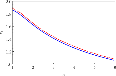
Figure 2: Radius of convergence of the series for the frequency as function of $\alpha$. The dashed and continuous lines are results from Padé and Hermite-Padé approximants.

References

- [1] K. N. Murty, M. A. S. Srinivas, and K. R. Prasad, “Approximate analytical solutions to the three-species ecological system”, J. Math. Anal. Appl. 145, 89-99 (1990).
- [2] T. Grozdanovski and J. J. Shepherd, “Approximating the periodic solutions of the Lotka-Volterra system”, ANZIAM J. 49, C243-C257 (2008).
- [3] J. F. Navarro, “A symbolic algorithm for the computation of periodic orbits in non-linear differential systems”, J. Adv. Appl. Math. 1, 160-174 (2016).
- [4] J. F. Navarro and R. Poveda, “Computation of periodic orbits in three-dimensional Lotka-Volterra systems”, Math. Meth. Appl. Sci. 40, 1-16 (2017).
- [5] R. E. Shafer, “On quadratic approximation”, SIAM J. Numer. Anal. 11, 447-460 (1974).
- [6] P. Amore, J. P. Boyd, and F. M. Fernández, “High order analysis of the limit cycle of the van der Pol oscillator”, arXiv:1711.09978 [math.NA].
- [7] T. M. Apostol, Calculus, Second ed. (Blaisdell, Waltham, 1969).