Quantization of the Szekeres System
Abstract
We study the quantum corrections on the Szekeres system in the context of canonical quantization in the presence of symmetries. We start from an effective point-like Lagrangian with two integrals of motion, one corresponding to the Hamiltonian and the other to a second rank Killing tensor. Imposing their quantum version on the wave function results to a solution which is then interpreted in the context of Bohmian mechanics. In this semiclassical approach, it is shown that there is no quantum corrections, thus the classical trajectories of the Szekeres system are not affected at this level. Finally, we define a probability function which shows that a stationary surface of the probability corresponds to a classical exact solution.
I Introduction
The silent universe is mathematically described by a set of six first-order differential equations following from the assumptions that i) the magnetic part of the Weyl tensor vanishes and ii) that the total matter source of the universe is described by a pressureless perfect fluid (irrotational dust fluid component) silent1 ; silent2 ; silent3 . In physical terms, the main property of the silent universe is that there is no information dissemination through gravitational or sound waves.
It is known that there exists a family of exact solutions for the field equations of the silent universe described as Szekeres geometries with line element of the form szek0
| (1) |
where and . There exists two families of solutions which correspond to the Friedmann–Lemaître–Robertson–Walker (like) geometries and the Kantowski-Sachs solutions kraj . One of the simplest solution in the Szekeres family is the Bondi-Tolman metric with line element
from which it is clear that the position of the singularity is space dependent, for more details see kraj .
In these solutions, the two components of the electric part of the Weyl tensor and the two components of the shear for the observer are equal respectively. While someone would expect that the “symmetry” between the different components of the Weyl tensor and the shear will generate an extra Killing field in the underlying manifold, it was shown in musta that the spacetimes coming from the Szekeres system are actually “partially” locally rotationally symmetric and not exactly. The particular interest of the scientific community on these geometries lies on their interesting properties and on the fact that they can be seen as inhomogeneous models sm00 ; sm00a0 ; sm00a ; sm01 ; this property renders these spacetimes proper for the description of FLRW spacetimes perturbations silent1 . Some recent results on the Szekeres geometries with one isometry and on their conformal symmetries can be found in ks1 ; ks2 .
In the following, we consider a Riemannian manifold with metric and a timelike four-vector field . Let be the energy momentum tensor of the matter source; the energy density is defined as and the field equations of the silent universe are reduced to a system of algebraic-differential equations with the algebraic equation being
| (2) |
and the first-order differential equations
| (3a) | |||
| (3b) | |||
| (3c) | |||
| (3d) | |||
| where denotes the directional derivative along , i.e. . The set of equations (3) is also well-known as Szekeres system szek0 ; barn1 . The parameter is the expansion rate of the observer, , while and are the shear and electric component of the Weyl tensor, in which the set of defines an orthogonal tetrad such that such that the components of tensors are scalar functions silent1 . The relation of the kinematical parameters and to the functions can be recovered by considering the decomposition of the line element (1) for an observer . Then, the expansion rate and the shear are carge1 | |||
| (4) |
It is important to note that the complete set of the gravitational field equations includes the differential equations in which is the decomposable tensor defined by the expression lesame . Thus, in general, the Szekeres system is a set of partial differential equations, except when the latter equations are satisfied identically. In this case, it reduces to a system of ordinary differential equations.
Recently, the conservation laws of the Szekeres system (3) were constructed with various methods in anszek and szek . In particular, in szek the method of Darboux polynomials and the Jacobi multiplier method were applied, while in anszek the symmetries and the movable singularities of the Szekeres system were studied. The novelty in the analysis of anszek is that an effective classical Lagrangian describing the system (3) was constructed. Furthermore, it was shown that the conservation laws of the Szekeres system follow from the application of Noether’s theorem on the aforementioned effective Lagrangian.
This work explores the effective Lagrangian of anszek at the quantum level by considering its canonical quantization with the use of symmetries chris2013 . The aim is to derive the physical properties after quantization in the context of Bohmian mechanics boh1 ; boh2 . The Bohmian approach to quantum theory is well suited for quantum cosmology, since it does not presupposes the existence of a classical domain as it is necessary for the Copenhagen interpretation for the measurement process to be defined. In addition, this interpretation results in the definition of deterministic trajectories on the configuration space. This allows the comparison of the classical versus semiclassical trajectories through the corresponding properties of each geometry. Hence, its application in cosmology has been considered before, see e.g. chris2013 ; pinto ; manto ; on1 ; palan .
II Classical Dynamics
In anszek the Szekeres system (3) was written in an equivalent form of a two second-order differential equations system
| (5a) | |||
| (5b) | |||
| where the variables are related to the energy density and the electric term as follows | |||
| (6) |
while the expansion rate and the shear are defined by the equations (3a), (3d) as . It was shown there that the dynamical system (5) can be derived by a variational principle with Lagrange function anszek
| (7) |
This Lagrangian is point-like and describes the motion of a particle in a two-dimensional space with line element
| (8) |
under the action of the effective potential The system (5) admits two integrals of motion, quadratic in the velocities; the first is the Hamiltonian function
| (9) |
since the system is autonomous, while the second one is the quadratic function
| (10) |
which can be constructed by the application of Noether’s theorem for contact symmetries anszek .
In order to proceed to the canonical quantization in the next section, we turn to the Hamiltonian formulation. The canonical momenta are defined by the Lagrangian (7) as
| (11) |
Then our conserved quantities are written in terms of the momenta correspondingly as
| (12) | |||
| (13) |
III Quantization and semiclassical analysis
The quantization is based on the idea of promoting the integrals of motion to operators, thus resulting to two eigenvalue equations. For simplicity, we choose to work in a new set of variables defined by , in which the point-like Lagrangian (7) takes the form
| (14) |
The equations of motion (5) become
| (15a) | |||
| (15b) | |||
| while the quadratic conserved quantity is written as . Hence, the Hamiltonian and the conserved quantity can be written in terms of the momenta as | |||
| (16a) | |||
| (16b) | |||
| The canonical quantization proceeds by promoting the Poisson brackets to commutators, and the variables on the phase space of to operators according to . This procedure leads to the time-independent Schrödinger equation111In which, denotes the Laplace operator . | |||
| (17a) | |||
| and the additional equation | |||
| (17b) | |||
| which follows from the quantization of (16b) ref1 ; ref2 ; ref3 . Contrary to the usual method applied in the literature, we used generalized symmetries, instead of point symmetries. | |||
The set of equations (17) provides, through the integrability conditions which must be satisfied for the consistency of the system, the following general solution for the wave function
| (18) |
where
| (19) | |||
| (20) |
The coefficients and are constants of integration. It is important to note that, due to the linearity of (17a), the general solution is the sum of the expression (18) on all possible values of the constant ; that is, .
III.1 Semiclassical analysis
In order to find the quantum effect on the classical system, we follow the Bohmian interpretation of quantum theory boh1 ; boh2 . In this context, the departure from the classical theory is determined by an additional term in the classical Hamilton-Jacobi equation,
| (21) |
known as quantum potential and defined by
| (22) |
denotes the amplitude of the wave function in polar form, and the Laplacian operator of (17a), see e.g. kim ; pinto ; manto ; Stu2 ; sing1 ; palan and references therein.
When the quantum potential is zero, the identification
| (23) |
is possible since the equation (21) becomes the classical Hamilton-Jacobi equation; these of course should give the classical solution of the Euler-Lagrange equations. If this classical definition for the momenta is retained even when , we can find semiclassical solutions which will differ from the classical ones.
In our case, we assume that the quantum corrections in the general solution (18) follow from the “frequency ” with the highest peak in the wave function. This is in agreement with the so-called Hartle criterion hartle ; at the same time, is the classical observable value, since it is an integration constant for the equations of motion. The assumption that the wave function has survival oscillatory term leads to the result that, in all possible cases, i.e. for or , as well as the subcases or , the quantum potential vanishes, thus providing no quantum corrections. Indeed, solving the set of the corresponding semiclassical equations (23) for our variables, we find the classical solution, since the phase function which now comes from the wave function is constant.
Hence, the wave function which followed from canonical quantization of the effective Lagrangian (14) indicates that the Szekeres universe remains “silent”, even at the quantum level. That means that because the quantum potential is zero, i.e. , the original system (3a)-(3d) remain the same. Hence, the classical solution corresponds to a silent universe.
III.2 Probability density
In this section we restrict ourselves to the case in which the wave function (18) with given by (19) and becomes
| (24) |
The case which is well behaved at the limits and leads to the following probability
| (25) |
where is the measure on the space of the configuration variables . After a change of the variable which induces the Jacobian of the transformation in the measure, the probability becomes
| (26) |
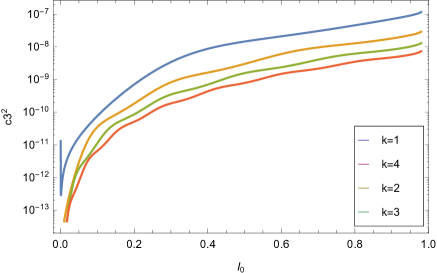
In order to exclude the case for the initial variables, we have introduced the constant as a cut-off. The normalization gives a quantized value for the constant . Its qualitative evolution is given in Fig. 1.
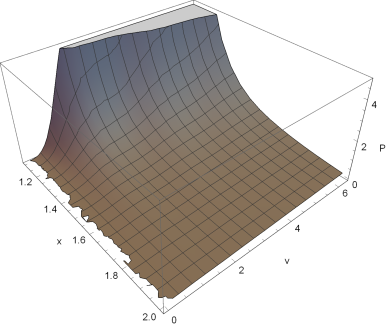
The qualitative behaviour of the probability function is given by
| (27) |
The surface diagram of this function is presented in Fig. 2, while the contour plot is presented in Fig. 3. The plots show that for the probability function reaches its minimum.
At this point, we would like to remind that the Szekeres system admits the exact solution , in which the integration constants and are zero anszek . The latter solution corresponds to an unstable critical point for the dynamical system (3) and it is very interesting that the conditions for the existence of the exact solution, i.e. and , lead to an extremum for the probability function. This might be related with the existense and the stability of the exact solution. The fact that the quantum probability has its minimum at the classical value is in accordance with the analysis of the probability extrema in dim1 where it was shown that the extrema of the probability lie on the classical values.


IV Conclusions
The purpose of this work was the study of the quantum behaviour of the Szekeres system in the context of the Bohmian interpretation to quantum theory. The quantization is based on an effective point-like Lagrangian which can reproduce the two dimensional system of second-order differential equations resulted from the initial field equations. This Lagrangian is autonomous, thus there exists a conservation law of “energy” corresponding to the Hamiltonian function. As for the extra contact symmetry, it leads to a quadratic in the momenta conserved quantity attributed to a Killing tensor of the second-rank. The two conserved quantities give two eigenequations at the quantum level, the Hamiltonian function being the Schrödinger equation.
The quantum behaviour is studied under the assumption that the wave function is peaked around its classical value. This leads to the lack of quantum corrections and the recovery of the classical solutions, thus leading to the conclusion that the Szekeres universe remains silent at the quantum level. Finally, for the particular case we study the probability function and relate one (unstable) exact solution with the existence of a minimum of this probability.
Acknowledgements.
A.P. acknowledges financial support of FONDECYT grant no. 3160121 and thanks Quatar University for the hospitality provided while part of this work was carried out. A.Z. acknowledges financial support by the grant GAČR 14-37086G.References
- (1) M. Bruni, S. Matarrese and P. Ornella, Astro. J. 445, 958 (1995)
- (2) H. van Elst, C. Uggla, W.M. Lesame, G.F.R. Ellis and R. Maartens, Class. Quantum Grav. 14, 1151 (1997)
- (3) H. Mutoh, T. Hirai and K-i Maeda, Phys. Rev. D 55, 3276 (1997)
- (4) N. Mustapha, G.F.R. Ellis, H. van Elst and M. Marklund, Class. Quantum Grav. 17, 3135 (2000)
- (5) M. Ishak and A. Peel, Phys. Rev. D 85, 083502 (2012)
- (6) K. Bolejko, Gen. Relativ. Grav. 41, 1737 (2009)
- (7) K. Bolejko and M.-N. Célérier, Phys. Rev. D 82, 103510 (2010)
- (8) D. Vrba and O. Svitek, Gen. Relativ. Grav. 46, 1808 (2014)
- (9) P.S. Apostolopoulos, Mod. Phys. Lett. A 32, 1750099 (2017)
- (10) I. Georg and C. Hellaby, Phys. Rev. D 95, 124016 (2017)
- (11) P. Szekeres, Commun. Math. Phys. 41, 55 (1975)
- (12) A. Barnes and R.R. Rowlingson, Class. Quantum Gravi. 6, 949 (1989)
- (13) A. Krasinski, Inhomogeneous Cosmological Models, Cambridge University Press, Cambridge (2010)
- (14) G.F.R Ellis and H. van Elst, Cosmological models (Cargèse lectures 1998), Kluwer Academic (1999) [gr-qc/9812046]
- (15) R. A. Sussman and K. Bolejko, Class. Quantum Grav. 29, 065018 (2012)
- (16) P.S. Apostolopoulos, Class. Quantum Grav. 34, 095013 (2017)
- (17) R. Maartens, W. Lesame and G.F.R. Ellis, Phys.Rev. D 55, 5219 (1997)
- (18) A. Paliathanasis and P.G.L. Leach, Phys. Lett. A 381, 1277 (2017)
- (19) A. Gierzkiewicz and Z.A. Golda, J. Nonl. Math. Phys. 24, 494 (2016)
- (20) N. Dimakis, A. Karagiorgos, T. Pailas, P.A. Terzis and T. Christodoulakis, Phys. Rev. D 95, 086016 (2017)
- (21) T. Christodoulakis, N. Dimakis, P.A. Terzis and G. Doulis, Phys. Rev. D 90, 024052 (2014)
- (22) A. Paliathanasis, M. Tsamparlis, S. Basilakos and J.D. Barrow, Phys. Rev. D 93, 043528 (2016)
- (23) T. Christodoulakis, N. Dimakis, P. A. Terzis, B. Vakili, E. Melas and T. Grammenos Phys. Rev. D 89, 044031 (2014)
- (24) P. Pinto-Neto and R. Colistete Jr., Phys. Lett. A 290, 219 (2001)
- (25) A. Zampeli, T. Pailas, P.A. Terzis and T. Christodoulakis, JCAP 05, 066 (2016).
- (26) N. Pinto-Neto, Found. Phys. 35, 577 (2005)
- (27) A. Paliathanasis, Mod. Phys. Lett. A 32, 1750206 (2017)
- (28) D. Bohm, Phys. Rev. 55, 166 (1952)
- (29) D. Bohm, Phys. Rev. 85, 180 (1952)
- (30) S.P. Kim, Phys. Lett A 236, 11 (1997)
- (31) F.T. Falciano, N. Pinto-Neto and W. Struyve, Phys. Rev. D 91, 043524 (2015).
- (32) R. Colistete, J.C. Fabris and N. Pinto-Neto, Phys. Rev. D 57, 4707 (1998)
- (33) J.B. Hartle . Plenum. Gravitation in Astrophysics: Cargèse, Proceedings of a Nato Advanced Study Institute on Gravitation in Astrophysics, Cargèse, France, B. Carter and J.B. Hartle (eds.) : New York (1986)
- (34) N. Dimakis, P.A. Terzis, A. Zampeli and T. Christodoulakis, Phys. Rev. D 94, 064013 (2016)