Measurement of the muon anti-neutrino double-differential cross section for quasi-elastic-like scattering on hydrocarbon at $E_{\nu}\sim 3.5$ GeV

Abstract

We present double-differential measurements of anti-neutrino quasi-elastic scattering in the MINERvA detector. This study improves on a previous single differential measurement by using updated reconstruction algorithms and interaction models, and provides a complete description of observed muon kinematics in the form of a double-differential cross section with respect to muon transverse and longitudinal momentum. We include in our signal definition zero-meson final states arising from multi-nucleon interactions and from resonant pion production followed by pion absorption in the primary nucleus. We find that model agreement is considerably improved by a model tuned to MINERvA inclusive neutrino scattering data that incorporates nuclear effects such as weak nuclear screening and two-particle, two-hole enhancements.

I Introduction

Although quasi-elastic neutrino interactions are a key signal process for accelerator-based oscillation experiments, models of these interactions on nuclei have large ($\sim 30\%$) uncertainties Andreopoulos et al. (2015); Abe et al. (2015a). These arise from several sources, including nucleon form factors and final state interactions wherein the produced particles interact further before exiting the primary nucleus. Final state interactions can also cause other processes such as resonant pion production to have a zero-meson final state that will appear with a quasi-elastic topology in a detector. Interactions with multi-nucleon states can similarly produce zero-meson final states.

These and similar sources of uncertainty on other processes dominate the systematic uncertainty budgets of the current oscillation measurements such as T2K Abe et al. (2017) and Nova Adamson et al. (2017) and will limit the reach of oscillation experiments such as DUNE Acciarri et al. (2015) if not further reduced. Because any one measurement of quasi-elastic scattering necessarily measures a superposition of these effects, lowering model uncertainties on individual parameters will require many different measurements to untangle the many unknowns.

In this article, we present a critical ingredient in this process: a double differential measurement of the anti-neutrino quasi-elastic cross section as a function of the transverse and longitudinal momentum of the final state muon. We include in our measurement events consistent with zero-meson final states arising from resonant pion production followed by pion absorption in the nucleus and from interactions on multi-nucleon states (frequently referred to as two-particle, two-hole or 2p2h). This ensemble of signal processes, which is defined precisely in Section VI, is referred to hereafter as “QE-like”. In addition to this primary result, we also present a number of auxiliary measurements including double-differential cross sections as a function of alternate variables, single differential projections, and comparisons of reconstructed energy near the event vertex to various models. The neutrino energy range of 1.5-15 GeV covered by this measurement is well matched to that of present and future neutrino oscillations experiments with baselines on the 1000 km scale, including MINOSMichael et al. (2008a), NOvAPatterson (2013), and DUNEGoodman (2015).

The measurement described here extends a previous measurement of anti-neutrino quasi-elastic scattering by MINERvA Fields et al. (2013) and is a companion to similar studies of neutrino scattering Fiorentini et al. (2013). The measurement complements other MINERvA QE-like studies that look in detail at the hadronic component of the final state Walton et al. (2015) and that study neutrino interaction cross sections as a function of nuclear mass Tice et al. (2014); Mousseau et al. (2016).

This article is organized as follows: Section II reviews the current status of neutrino-nucleus QE-like scattering models. Sections III and IV review the MINERvA experiment and simulation. Event reconstruction and selection are discussed in Sections V and  VI. The cross section extraction procedure and systematic uncertainties are detailed in Sections VII and VIII. The results and comparisons with models are presented in Section IX, and the article is summarized in Section X. The Appendices present additional results, including cross sections with alternate signal definitions; those planning to use the data are encouraged to use the supplementary materials, which provide higher numerical precision.

II Theory of QE-like Interactions

In charged-current quasi-elastic scattering on free nucleons, an incoming muon anti-neutrino interacts with a target proton, exchanging a $W^{\pm}$ boson to knock out a neutron and leave a positively charged muon in the final state:

$$\bar{\nu}_{\mu}+p\to\mu^{+}+n$$ (1)

In this case, it is possible to reconstruct certain characteristics of the interaction using only the kinematics of the outgoing charged lepton assuming the initial-state nucleon is at rest. For a nucleon bound within a nucleus, the incoming neutrino energy and the four-momentum transfer, $Q^{2}$, can be estimated as:

$$E_{\nu}^{QE}=\frac{m_{n}^{2}-(m_{p}-E_{b})^{2}-m_{\mu}^{2}+2(m_{p}-E_{b})E_{\mu}}{2(m_{p}-E_{b}-E_{\mu}+p_{\mu}\cos\theta_{\mu})}$$ (2)

$$Q^{2}_{QE}=2E_{\nu}^{QE}(E_{\mu}-p_{\mu}\cos\theta_{\mu})-m_{\mu}^{2}$$ (3)

where $E_{b}$ is the initial state nucleon’s binding energy, taken to be 30 MeV, as described in Fields et al. (2013), $E_{\nu}$ and $E_{\mu}$ are the neutrino and muon energy, $p_{\mu}$ and $\theta_{\mu}$ are the muon’s momentum and angle with respect to the neutrino, and $m_{\mu}$, $m_{n}$, $m_{p}$ are the mass of the muon, neutron and proton. The ${QE}$ subscript and superscript here and throughout the remainder of this article denotes quantities computed under an assumption of a quasi-elastic hypothesis with the initial state nucleon at rest.

In the case of a bound nucleon, Fermi motion and nucleon correlations mean that the initial state nucleon is not at rest, making the $QE$ kinematic variables only estimates of the true values. The final state interpretation can also be affected, as an ejected nucleon may interact with other nucleons while escaping the nucleus. Other interactions such as resonant pion production can be modified by final state nuclear effects to have no pions in the final state, thus appearing QE-like. Similarly, interactions with correlated pairs of nucleons can also produce final states that appear quasi-elastic. All of these nuclear effects can cause quasi-elastic neutrino interactions on heavy nuclei to differ substantially from those on free nucleons. In this section, we discuss the quasi-elastic scattering from a free nucleon, and several contemporary theories that attempt to model the impact of the nuclear environment. More detail can be found in Patrick (2016).

Quasi-elastic Anti-neutrino Scattering on Free Nucleons

Because the internal structure of the initial- and final-state nucleons is governed by the non-perturbative regime of QCD, it is not possible to make a precise ab initio calculation of the neutrino-nucleon quasi-elastic cross-section; it may instead be described by nucleon form factors. In the 1972 review article of C. Llewellyn-Smith Llewellyn Smith (1972), the differential quasi-elastic cross section is expressed as a function of two vector, one axial-vector, one pseudoscalar and two second-order form factors. All but the axial form factor are known from electron-nucleon scattering measurements. The axial form factor must be taken from neutrino scattering or pion electro-production measurements, and is typically parametrized as a dipole:

$$F_{A}(Q^{2})=\frac{g_{A}}{(1+\frac{Q^{2}}{M_{A}^{2}})^{2}}.$$ (4)

The value of the axial form-factor at $Q^{2}=0$, has been measured through beta-decay experiments Wilkinson (1982); Maerkisch and Abele (2014), leaving one free parameter, the axial mass $M_{A}$. Deuterium and hydrogen bubble chambers Miller et al. (1982); Kitagaki et al. (1990) have measured the value of $M_{A}$ on free or quasi-free nucleons. An average value of $M_{A}=1.014\pm 0.014\text{\>GeV/}c^{2}$ was extracted by Bodek et al. Bodek et al. (2008) in 2008. Modern experiments on heavy nuclei have favored higher values of $M_{A}$  Aguilar-Arevalo et al. (2010); Adamson et al. (2015a); Abe et al. (2015b), and the discrepancy between these and the deuterium experiments has been attributed to insufficiencies in the nuclear models used to extract the axial mass on heavy nuclei. Alternate parameterizations of the dipole form factor are also available. In particular, a more general “z-expansion” parameterization Bhattacharya et al. (2011) has been widely adopted in flavor physics and was recently implemented in neutrino event generators.

Scattering from Nuclei

When simulating quasi-elastic scattering in heavy nuclei, the most commonly used nuclear model is the Relativistic Fermi Gas (RFG) model proposed by Smith and Moniz Smith and Moniz (1972), in which scattering from a nucleon in a nucleus is treated as if the incoming lepton scatters from an independent nucleon (the “impulse approximation”). However, in the case of the RFG, the target nucleon is not stationary, but has a momentum consistent with the Fermi distribution. Thus the cross section for scattering off the nucleus is replaced by an incoherent sum of cross sections for scattering off of individual nucleons, with the remaining nucleus (depleted by 1 nucleon) as a spectator.

The Local Fermi Gas (LFG) model is a extension to the RFG model in which a local density approximation Negele (1970); Maruhn et al. (2009) is used, so that instead of using a constant average field for the whole nucleus, the momentum distribution is dependent on a nucleon’s position within the nucleus. This gives a Fermi motion distribution that is not sharply peaked at the momentum limit and is both more natural and reproduces the measured peak of the distribution.

Spectral functions can be also used to improve the Relativistic Fermi Gas model Cenni et al. (1997). The Hamiltonian for a large nucleus is so complicated that it is impractical to try to solve the many-body Schrödinger equation for the entire nucleus. However, if a mean field is used to replace the sum of the individual interactions, a spectral function can be constructed that represents the probability of finding a nucleon with momentum and removal energy within the nucleus. There are a number of non-Fermi-gas approaches Benhar et al. (2005); Jachowicz et al. (2002); Pandey et al. (2015); Lovato et al. (2015); Gonzalez-Jimenez et al. (2014); Megias et al. (2016).

Multi-Nucleon Correlations

The models described above, which treat individual nucleons independently, do not fully take into account the nature of the nuclear force, which has a short range with a repulsive core Arrington et al. (2012). Interactions between two (or more) spatially close nucleons can give the individual nucleons very high momenta, far above the Fermi momentum. Electron scattering Egiyan et al. (2006) data indicate that approximately 20% of the nucleons in carbon atoms are part of correlated pairs. These experiments have observed ejected nucleons consistent with knocked-out partner nucleons Shneor et al. (2007); Subedi et al. (2008), with 90% of those pairs found to be proton-neutron pairs, with the remainder being $nn$ and $pp$ pairs. In the case of $np$ pairs, it is expected that charged current QE-like anti-neutrino scattering on protons within a correlated pair would tend to produce two neutrons – the expected neutron produced by the QE-like interaction, plus the knocked out neutron partner.

The impact of multi-nucleon states in the initial state has been modeled in a number of ways. Bodek and Ritchie’s modification to the Relativistic Fermi Gas model Bodek and Ritchie (1981) adds a high-momentum tail to the RFG’s momentum distribution, based on the nucleon-nucleon correlation function and fits to data as explained in Gottfried (1963). While this method attempts to provide a realistic initial momentum distribution, it does not include any model for the ejection of paired nucleons.

Going a step further, Bodek, Budd and Christie Bodek et al. (2011) have developed a “transverse enhancement model” (TEM). They fit inclusive electron scattering data Carlson et al. (2002); Mamyan (2010), modifying the nucleon magnetic form factors to accommodate the enhancement of the transverse response observed in those data. The resulting form factor modifications plus an unmodified axial vector form factor were then used to predict neutrino-nucleus scattering cross sections, producing results that were consistent with both low-energy data from MiniBooNE Aguilar-Arevalo et al. (2010) and high-energy results from NOMAD Lyubushkin et al. (2009). The TEM fit does not attempt to model additional knocked-out nucleons in either the electron or neutrino case. Those empirical fits, when combined with different expressions O’Connell et al. (1972) for how the structure functions should be related, and attaching a two-nucleon knockout are used in the GiBUU generator.

While the approaches described above are empirical models that ascribe effects observed in electron scattering to multi-nucleon processes and then attempt to predict the effect they might have on neutrino scattering, 2p2h models attempt to predict multi-nucleon effects in neutrino scattering from first principles. These models consider pairs of nucleons connected by the exchange of virtual pions and rho mesons Van Orden and Donnelly (1981). There has been a recent dramatic expansion of work on 2p2h models, such as those of Marteau/Martini Martini et al. (2009), IFIC Valencia group Nieves et al. (2011), the SuSA group Gonzalez-Jimenez et al. (2014); Megias et al. (2016), and the Gent group Van Cuyck et al. (2017). As of this writing, the IFIC Valencia model is implemented in GENIE, NuWro, and NEUT for the CC process. Empirical versions related to the TEM fits to electron scattering data are also available in GENIE (without two-nucleon knockout) and GiBUU (with two-nucleon knockout). Finally, there is a version that implements a simple empirical shape in W and Q2 developed for use in electron scattering codes Jr. and O Connell (1988) to generate events as an option in GENIE Katori (2015).

Long-range correlations between nucleons are typically modeled using an approach known as the random-phase approximation (RPA) Morfín et al. (2012). It is based on the phenomenon, observed in $\beta$-decay and muon capture experiments, that the electroweak coupling can be modified by the presence of strongly-interacting nucleons in the nucleus, when compared to its free-nucleon coupling strength, similar to the screening of an electric charge in a dielectric. The RPA approach affects cross-section predictions at low energy transfers (and low $Q^{2}$), where a quenching of the axial current reduces the cross section compared to the RFG prediction. It also introduces a small cross section enhancement at intermediate $Q^{2}$. Multiple RPA models are available within generators, including those of Nieves Nieves et al. (2004), Martini Martini et al. (2009), Graczyk and Sobczyk Graczyk and Sobczyk (2003), and Singh Singh and Oset (1992). There is also discussion of the interplay between RPA with the Fermi gas and beyond-the-Fermi-gas models Martini et al. (2016) Nieves and Sobczyk (2017).

Final-State interactions

Non-quasi-elastic processes that undergo final-state interactions within the nucleus can have QE-like final states. For example, there are three possible anti-neutrino charged-current resonant pion production processes:

$$\bar{\nu}_{\mu}p \to\mu^{+}p\pi^{-}$$ (5)

$$\bar{\nu}_{\mu}p \to\mu^{+}n\pi^{0}$$ (6)

$$\bar{\nu}_{\mu}n \to\mu^{+}n\pi^{-}$$ (7)

In such events, there is a $\sim$20% possibility that the pion will be absorbed before it exits the nucleus, leaving a QE-like final state of a single muon and one or more nucleons.

Nearly all available models of final state interactions are Intranuclear Cascade (INC) models in which final state hadrons are individually propagated through the nucleus with some probability of undergoing interactions such as absorption or inelastic scattering with the nuclear medium. The details of the interactions vary significantly across different models (typically implemented as part of an event generator such as GENIE Andreopoulos et al. (2015) or NEUT Hayato (2009)), but all are tuned to hadron scattering data. Some generators (including GENIE) also provide effective cascade models wherein the cascade of interactions that particles may undergo as they traverse a nucleus is modeled as a single interaction. At least one alternative to INC models exists in the form of a semi-classical nuclear transport model implemented as part of GiBUU Leitner et al. (2009).

III MINERvA Experiment

The MINERvA (Main INjector ExpeRiment $\nu$-A) experiment is situated in the NuMI (Neutrinos at the Main Injector) neutrino beam at Fermilab. The detector and beam are described in detail in Aliaga et al. (2014) and Adamson et al. (2015b); this section summarizes their main features, focusing on the components relevant to this study.

The NuMI neutrino beam

Fermilab’s NuMI beam uses 120 GeV/c protons from the Main Injector, which impinge on a 1 meter long graphite target. The resulting pions and kaons are focused by a pair of movable parabolic horns. The horn current polarity can be set to focus positively or negatively charged mesons, which decay in a 675m-long decay pipe, producing muons and neutrinos. An absorber removes any remaining hadrons from the beam and 200 meters of rock filter out muons, leaving a beam of primarily neutrinos or anti-neutrinos, depending on the horn current polarity.

For the low energy beam configuration used in this work, the peak beam energy was approximately 3 GeV and the horns were configured to focus negative particles. We use data recorded between November 5, 2010 and February 24, 2011, corresponding to $1.020\times 10^{20}$ protons on target (POT). The Monte Carlo simulation described in the next section corresponds to $9.247\times 10^{20}$ POT.

MINERvA Detector

The MINERvA detector is composed of an inner detector (ID) and an outer detector (OD). The most upstream portion of the ID consists of active scintillator planes interspersed with passive nuclear targets. This region is used for studies of the A-dependence of neutrino interaction cross sections, but is not used in the work described here. Immediately downstream of the nuclear target region is the central tracker, followed by electromagnetic and hadronic calorimeters (ECAL and HCAL).

The tracker is composed of 124 active scintillator planes, each consisting of 127 strips of doped polystyrene scintillator with a titanium dioxide coating. The strips have a triangular cross section $17$ mm (height) by $33$ mm (base) and vary in length between 122 and 245 cm depending on position within the plane. Each scintillator plane is installed in one of three orientations, X, U or V. In the X orientation, the strips are vertical. Strips in the U or V planes are oriented at $\pm 60^{\circ}$ with respect to the strips in the X planes. Each module in the active tracker region consists of two planes of scintillator strips, alternating between UX and VX configurations. A 2mm-thick lead collar covers the outermost 15 cm of each plane, forming the side electromagnetic calorimeter.

The downstream ECAL consists of ten modules that are similar to tracker modules, except that the 2mm-thick lead collar is replaced by a 2mm-thick sheet of lead covering the plane. The 20 hadronic calorimeter (HCAL) modules, downstream of the ECAL, each contain only one plane of scintillator, followed by a 2.54 cm-thick plane of steel.

Light produced in the scintillator is collected by a 1.2 mm diameter wavelength-shifting (WLS) optical fiber inserted in a hole passing along the length of the strip and transmitted by the optical fibers to Hamamatsu H8804MOD-2 photomultiplier tubes (PMTs), as described in Aliaga et al. (2014). The full detector has 507 PMTs, each of which consists of 64 pixels. The PMTs are read out via a data acquisition system that is described in detail in Perdue et al. (2012). Raw PMT counts are transformed into estimated energy deposited in the strip via the calibration chain also described in Perdue et al. (2012). The intrinsic time resolution is $~{}4$ ns.

The MINOS Near Detector

The MINOS Near Detector Michael et al. (2008a) is located 2 meters downstream of MINERvA, and is used to measure the charge and momentum of muons exiting the back of MINERvA. The 1 kTon MINOS detector is composed of 2.54 cm-thick steel planes, interspersed with 1 cm-thick layers of scintillator. The scintillator planes are formed from 4.1 cm-wide scintillator strips, with orientation of the strips alternating between $+45^{\circ}$ and $-45^{\circ}$ to the vertical in successive planes. The first 120 planes are instrumented for fine sampling; in this region, every fifth steel plane is followed by a fully-instrumented scintillator plane, while all other steel planes are followed by a partially-instrumented scintillator plane. The coarse-sampling region, further downstream, has only the fully-instrumented scintillator every five planes; there are no partial scintillator planes in this region. The MINOS detector is magnetized by a coil that runs in a loop passing through the detector, generating a toroidal field with an average strength of 1.3 T.

IV MINERvA Simulation

Beam Flux Simulation

MINERvA’s simulation chain begins with G4Numi Aliaga Soplin (2016), a Geant4 Agostinelli et al. (2003a) based simulation of the NuMI beamline from primary proton beam to the MINERvA detector. The FTFP_BERT inelastic scattering model of Geant version 4.9.2.p03 is used. This raw simulation is found to disagree with existing hadroproduction data from the NA49 Alt et al. (2007) and other experiments Barton et al. (1983); Lebedev (2007), and is therefore corrected so that both differential and total interaction cross sections in the simulation match these external datasets. Version 1 of the PPFX package is used to implement these corrections Aliaga et al. (2016).

We also use neutrino-electron scattering data collected in the MINERvA detector with the beamline in neutrino mode (focusing positive pions) as an independent constraint on the flux model, as described in Park et al. (2016). This constraint lowers the predicted neutrino flux by 2-4% depending on neutrino energy. While an equivalent measurement is not available for the anti-neutrino running mode due to low statistics for the $\bar{\nu}-e$ process in that configuration, the known correlations between the neutrino and anti-neutrino fluxes are used to apply this constraint to the anti-neutrino flux distribution. As shown in Fig. 1, applying the constraint results in a 1-3% decrease in the anti-neutrino flux prediction.

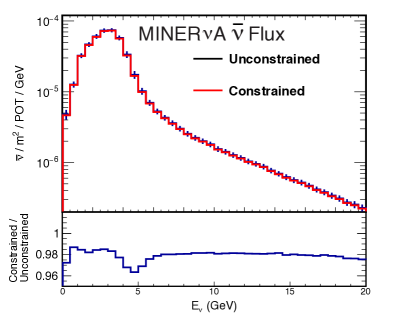
Figure 1: NuMI flux distributions averaged over the MINERvA fiducial volume for anti-neutrinos as a function of energy, with and without a neutrino-electron scattering constraint. The top plot shows the constrained (red) and unconstrained (black) distributions, which are separate by less than the line width. The lower plot shows the ratio of the constrained to unconstrained values. The units are anti-neutrinos/proton on target/m².

Neutrino Event Generation

MINERvA uses a modified version of the GENIE neutrino interaction event generator Andreopoulos et al. (2010) version 2.8.4 to model physics processes within the primary interaction nucleus. Simulated event distributions using this generator, with data constraints described in section VII, are used to estimate background levels, resolution effects, acceptance and efficiency.

GENIE models the nucleus using the Relativistic Fermi Gas model Smith and Moniz (1972) incorporating the Bodek-Ritchie high-momentum tail Bodek and Ritchie (1981) that simulates short-range correlations. For carbon, the maximum momentum for Fermi motion is taken as $k_{F}=0.221$ GeV/c, and Pauli blocking is also included. Quasi-elastic cross sections follow Llewellyn-Smith’s prescription. Vector form factors are modeled by default using the BBBA05 model Bradford et al. (2006). For the axial vector form factor $f_{A}$, a dipole form is used, with $f_{A}(0)=1.2670$ and axial mass $M_{A}=0.99$  GeV/c² Kuzmin et al. (2008).

GENIE uses the Rein-Sehgal model Rein and Sehgal (1981) to simulate baryon resonance production, which provides cross sections for 16 different resonance states. The resonant axial mass $M_{A}^{RES}$ is taken to be 1.12 GeV/c². DIS cross sections are calculated with an effective leading order model with a low-$Q^{2}$ modification from Bodek and Yang Bodek et al. (2005). Hadronic showering is modeled with the AGKY model Yang et al. (2007). The Bodek-Yang model also describes other low-energy non-resonant pion production processes. Re-scattering of nucleons and pions in the nucleus is simulated using the INTRANUKE-hA intra-nucleon hadron cascade package Dytman (2007). While the resonant interactions described earlier account for the majority of pion production, other inelastic processes, as described by Bodek-Yang Bodek et al. (2005) are also possible. In particular non-resonant pion production followed by FSI can produce a QE-like signature.

In addition to the basic processes simulated in GENIE 2.8.4 we also apply three additional corrections. First, we reweight quasi-elastic events as a function of the energy and 3-momentum transfers $q_{0}$ and $q_{3}$ to include the Random Phase Approximation model as predicted by the Valencia model of Nieves et al. Nieves et al. (2004) and implemented for MINERvA Gran (2017). Fig. 2 shows the $Q^{2}$ dependence of this correction. Second, QE-like interactions on multi-nucleon pairs are simulated using the Valencia IFIC model. We modify this model to match MINERvA inclusive neutrino scattering data reported in  Rodrigues et al. (2016a), which enhances this contribution by approximately 60%,

Finally, the normalization of non-resonant pion production is reduced to 43% of the default GENIE 2.8.4 prediction, based on a fit to pion-production data on deuterium from bubble-chamber experiments at Argonne and Brookhaven National Laboratories Rodrigues et al. (2016b). We reduce the uncertainty on the normalization of this process to 5%, based on the same data fit. This modified version of GENIE 2.8.4 is hereafter referred to as MINERvA-tuned GENIE.

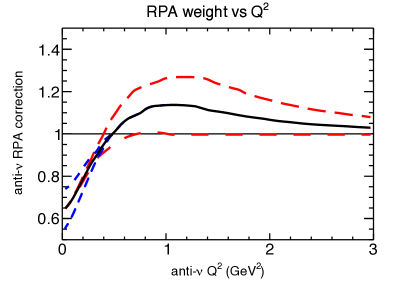
Figure 2: Random Phase Approximation correction projected as a function of generated $Q^{2}$. The solid black curve indicates the central value from the relativistic calculation. The short dashed blue lines indicate uncertainties from low $Q^{2}$ processes suggested by the application of the model of Nieves et al. to muon capture data, and the long dashed red lines a higher $Q^{2}$ uncertainty estimated from the difference between the relativistic and non-relativistic calculations.

Detector Simulation

The Geant4 toolkit Agostinelli et al. (2003b) v4.9.4p02 with the QGSP_BERT physics list is used to simulate propagation through the material of the detector and has been validated using a scaled-down version of the MINERvA detector in a test beam Aliaga et al. (2015). The optical and electronics systems are also simulated, which allows the energy depositions recorded by Geant4 to be converted to a simulated readout that can be analyzed as if it were MINERvA data. This simulated data is overlaid with actual data to include the effects of multiple neutrino interactions, noise and dead-time, which is a result of the $\sim 150$ ns digitization window following activity above threshold, during which additional deposits will not be recorded.

V Event Reconstruction

Calibrated energy depositions in the scintillator strips (referred to subsequently as ‘hits’) are reconstructed into anti-neutrino interaction candidates through a series of steps. First, the ensemble of hits collected over the $10\mu$s long NuMI beam spill are grouped into time slices corresponding to individual neutrino interactions. Hits within the same time slice are then collected into clusters that are adjacent in strip space and contained within the same scintillator plane. The position of the cluster is taken to be the energy-weighted average of the hit (strip) positions; the cluster time is set to the time of the highest-energy hit.

Track Reconstruction

Track reconstruction begins by collecting clusters within a single time slice into ‘seeds’ containing three clusters in consecutive planes of the same (X,U or V) orientation that fit to a straight line. Seeds are merged into track candidates within each view (X, U and V), and candidates are formed into 3-dimensional tracks, which are fitted with a Kalman filter routine R. Frühwirth (1987); R. Luchsinger and C. Grab (1993), in combination with additional untracked clusters in planes adjacent to the track. This allows tracks to be extrapolated through areas of high activity (such as a hadron shower). This algorithm is then repeated to identify additional charged particles in the event until no further tracks are identified.

A similar reconstruction algorithm is performed in parallel in the MINOS detector, where time slices are selected by looking at hits clustered in space and time. The hits in a given time slice are then formed into clusters, which are grouped into tracks if their positions are correlated. Each track’s path is then estimated using a Kalman filter; unlike in MINERvA, MINOS tracks curve due to the detector’s magnetic field. For tracks stopping within the detector and not entering the coil, the track’s momentum is estimated via range; otherwise, the momentum is estimated via curvature through the Kalman fit. For the data considered here, MINOS’s magnet was configured to focus positive muons.

Once tracks have been formed in both MINERvA and MINOS, they are then matched between the two detectors. MINOS tracks are matched to MINERvA muons when activity is measured in the last five planes of MINERvA, and a track starts in the first four planes of MINOS within 200ns of the MINERvA track time. The MINERvA track is extrapolated forwards to the first MINOS plane, and the MINOS track is extrapolated back to the last plane of MINERvA. The point of closest approach between the two tracks is required to be less than 40 cm.

The final step of track reconstruction is known as muon “cleaning”. MINOS-MINERvA matched tracks are deemed to be muons. Energy beyond the expected deposition of a minimum-ionizing particle is removed from the muon track and added to the ensemble of unmatched clusters considered for further reconstruction.

Recoil energy reconstruction

We refer to final-state energy not associated with the muon track as “recoil energy”. In this study we consider only energy deposited in the tracker and ECAL portions of the detector, and further require recoil cluster times to be between 20 ns before and 35 ns after the path-length-corrected average time of clusters on the muon track. We also exclude all clusters likely to be due to PMT cross talk and clusters within 10 cm of the muon vertex from the recoil energy sum, to minimize dependence on simulations of energy near the vertex, which are sensitive to details of final-state and multi-nucleon interactions. Energy in all remaining clusters is summed and calorimetrically corrected:

$$E_{\text{recoil}}\equiv\sum\limits_{i}C^{sd}_{i}E_{i}$$ (8)

where $C^{sd}_{i}$ is a calorimetric constant obtained from the simulation for sub-detector $i$ that corrects for the passive material fraction in that sub-detector (1.22 for the tracker and 2.013 for the ECAL).

VI Event Selection

Before identifying selection criteria for isolating signal events, it is necessary to clearly define what is meant by “signal”. For MINERvA’s first studies of quasi-elastic scattering Fields et al. (2013); Fiorentini et al. (2013), we attempted to measure events in which the underlying neutrino-nucleon interaction was quasi-elastic, regardless of how those events were modified by final state interactions. Several other experiments have recently published measurements Aguilar-Arevalo et al. (2013, 2010); Abe et al. (2015b) of QE-like events with a final state of an appropriately-charged muon, plus nucleons. In this case, resonant pion production events where the pion is absorbed become part of the signal to be measured. However in MINERvA’s scintillator tracker, which is able to resolve proton tracks above a kinetic energy of 120 MeV, and to detect the energy of lower energy particles, this definition is not ideal. For this study, we define our signal to be events that are anti-neutrino charged-current events occurring in the MINERvA tracker fiducial volume, have post-FSI final states without mesons, prompt photons above nuclear de-excitation energies, heavy baryons, or protons above our proton tracking kinetic energy threshold of 120 MeV, and include a muon emitted at an angle with respect to the beam of less than 20 degrees, $1.5$ GeV$<p_{\parallel}<15$ GeV and $p_{T}<1.5$ GeV (matching the region where tracks can be reconstructed in both MINERvA and MINOS with well-reconstructed momentum). This is similar to the QE-like (often called CC0Pi) definitions used by other experiments Aguilar-Arevalo et al. (2010); Abe et al. (2016), modified slightly to correspond to MINERvA’s acceptance, which is poor for events with high angle muons, very low or very high momentum muons, but able to reject high momentum protons. We also report alternate results where the signal definition consists of interactions that were initially generated in GENIE as quasi-elastic (that is, no resonant or deep inelastic scatters, but including scatters from nucleons in correlated pairs with zero-meson final states), regardless of the final-state particles produced.

We begin the event selection by identifying time slices containing at least one track reconstructed in the MINERvA detector and matched to a track in the MINOS detector as described in Section V. This provides a high purity sample of charged-current events. To isolate anti-neutrino event candidates, we further require that the charge-momentum ratio (q/p) returned by the MINOS Kalman fit be positive. Because we also require no visible proton in the final state, the remaining neutrino contamination in our samples is quite low - 0.6% in simulation - and is accounted for in the acceptance calculation. Because MINERvA experiences some dead time after an event has been recorded, we further require that no more than one strip immediately upstream of the track vertex (projected along the track direction) or immediately adjacent to these strips be dead at the time of the neutrino event. This reduces candidates arising from through-going muons generated upstream of the detector to less than 0.1% . We require the reconstructed interaction vertex to be within the fiducial volume of our detector; the vertex must be within a hexagon of apothem 850 mm and fall within modules 27 to 80, inclusive, corresponding to 108 tracking planes. We also require our reconstructed muon longitudinal momentum to be less than 15 GeV. This removes very energetic, forward-going muons that have poor energy reconstruction in MINOS.

To reduce backgrounds from non-QE-like events, we require that no tracks other than the muon track be reconstructed between 20 ns before and 35 ns after the muon track (the same time window used for recoil energy reconstruction). This reduces backgrounds from events with charged pions, particularly at high $Q^{2}_{QE}$ where the recoil cut described below is very loose, while the narrow time window minimizes the likelihood that signal events are rejected due to overlapping neutrino interactions.

Charged pions and high-energy protons do not always leave reconstructable tracks; they do, however, deposit clusters of energy in the detector. We therefore consider recoil energy, reconstructed as described in Section V and shown in Fig. 3. We find that the purity the QE-like sample depends on both the recoil energy and on the $Q^{2}_{QE}$ of the interaction, with high $Q^{2}_{QE}$ interactions having larger recoil (see Fig. 4). We therefore apply a $Q^{2}_{QE}$ dependent cut on the recoil energy:

$$E_{recoil} < \max(0.08,0.03+0.3\times Q^{2}_{QE})\mathrm{\>GeV\>and}$$

$$E_{recoil} < 0.450\mathrm{\>GeV}$$

where $Q^{2}_{QE}$ is in units of GeV².

Figure 3: Recoil energy for data (points) and simulation (colors, POT-normalized to data). In the simulation, signal events include both quasi-elastic events (purple), 2p2h scatters (green) and resonant or DIS events (pink and red) with a QE-like signature. The backgrounds consist of quasi-elastic and 2p2h events with non-QE-like signature (hatched purple and green), and non-QE events (resonant and DIS) without a QE-like signature (hatched pink and red). All cuts except the recoil cut are applied.

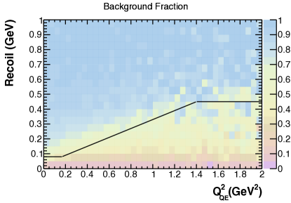
Figure 4: Simulated QE-like background fraction before the recoil cut, in bins of $Q^{2}$ and recoil energy. The line shows the $Q^{2}$ dependent recoil energy selection used to optimize efficiency and purity.

VII Cross Section Extraction

The double-differential cross section versus variables $x$ and $y$ in bin $(i,j)$ is constructed using:

$${\left(\frac{\mathop{d^{2}\sigma}}{\mathop{dx}\mathop{dy}}\right)}_{ij}=\frac{U\left(N_{\alpha\beta}-N^{bkgd}_{\alpha\beta}\right)}{\epsilon_{ij}(\Phi T)(\Delta x_{i})(\Delta y_{j})}$$ (9)

Where $N_{\alpha\beta}$ is the number of data events reconstructed in bin $(\alpha,\beta)$, $N^{bkgd}_{\alpha\beta}$ is the estimated number of background events reconstructed in bin $(\alpha,\beta)$, $U$ is an unfolding operation transforming reconstructed bin $(\alpha,\beta)$ to true bin $(i,j)$, $\epsilon_{ij}$ is the product of reconstruction efficiency and detector acceptance for events in true bin $(i,j)$, $\Phi$ is the flux of incoming anti-neutrinos (either integrated or for the given bin, as described later), $T$ is the number of scattering targets (here, the number of nucleons), and $\Delta x_{i}$ ($\Delta y_{j}$)is the width of bin $i$ ($j$).

We report our primary cross section measurement in bins of muon transverse ($p_{T}$) and longitudinal momentum ($p_{\parallel}$) with respect to the neutrino beam direction. We choose these as our primary results as they are quantities that we have directly measured. For comparison with other experiments, we also report auxiliary measurements vs. $Q^{2}_{QE}$ and $E_{\nu}^{QE}$, both reconstructed in the quasi-elastic hypothesis from the muon kinematics (see Eqs. 2 and 3). The bin boundaries are shown in Table 1.

$p_{T}$ (GeV/c)	$0,0.15,0.25,0.4,0.7,1.0,1.5$
$p_{\parallel}$ (GeV/c)	$1.5,2.0,2.5,3.0,3.5,4.0,5.0,6.0,8.0,10.0,15.0$
$Q^{2}_{QE}$ (GeV2)	$0.0,0.025,0.05,0.1,0.2,0.4,0.8,1.2,2.0$
$E_{\nu}^{QE}$ (GeV)	$1.5,2.0,2.5,3.0,3.5,4.0,5.0,6.0,7.0,8.0,10.0$

Table 1: Bin boundaries.

Two bins at highest $p_{T}$ and lowest $p_{\parallel}$ and four bins at highest $Q^{2}_{QE}$ and lowest $E_{\nu}^{QE}$ are not reported due to poor acceptance in those regions. Note that, as $Q^{2}_{QE}$ and $E_{\nu}^{QE}$ are reconstructed from the muon kinematics, they are both functions of both $p_{\parallel}$ and $p_{T}$. Figure 5 shows lines of constant $Q^{2}_{QE}$ and $E_{\nu}^{QE}$, projected onto the $p_{\parallel}$/$p_{T}$ phase space. For most of the region considered by this analysis, $E_{\nu}^{QE}$ correlates fairly well with $p_{\parallel}$, and $Q^{2}_{QE}$ with $p_{T}$ . This simplification breaks down at high $p_{T}$ and low $p_{\parallel}$. For both versions of the double-differential cross sections, we also report projections onto each axis, resulting in one-dimensional distributions of $p_{T}$, $p_{\parallel}$, $Q^{2}_{QE}$, and $E_{\nu}^{QE}$.

For the single differential cross section versus $E_{\nu}^{QE}$, we report a flux-weighted cross section, where each bin has been divided by the flux integrated over the energy range of that bin only, rather than the entire anti-neutrino flux integrated over all energies. Note that care must be taken in interpreting this quantity, as $E_{\nu}^{QE}$ does not correspond exactly to true anti-neutrino energy.

Figure 5: Relationship between $E_{\nu}^{QE}$ and $Q^{2}_{QE}$ in the quasi-elastic hypothesis, and muon kinematic variables $p_{T}$ and $p_{\parallel}$. The dashed lines show constant values of $E_{\nu}^{QE}$(blue) and $Q^{2}_{QE}$ (green) corresponding to our $E_{\nu}^{QE}$ and $Q^{2}_{QE}$ bin boundaries, which are given in Table 1.

A total of 17,621 interactions pass our reconstruction cuts for data. Distributions of these events versus muon $p_{T}$, in bins of $p_{\parallel}$ are shown in Fig. 6.

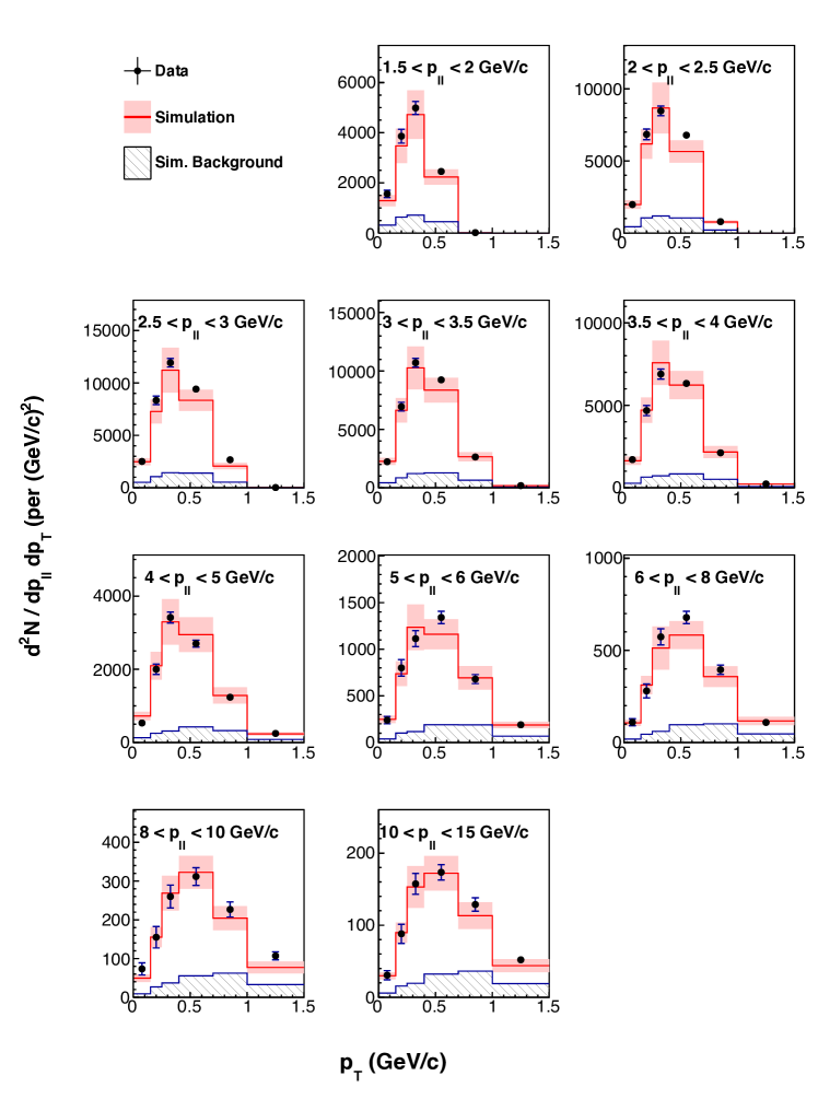
Figure 6: Reconstructed event counts vs. muon transverse momentum, in bins of muon longitudinal momentum. Uncertainties on the data are indicated by error bars; uncertainty on the Monte Carlo is indicated by a pink shaded bar. The data uncertainty is statistical; the Monte Carlo simulation includes all sources of systematic uncertainty, including uncertainties on the GENIE signal model. The estimated background contribution is shown by the hatched area.

Background subtraction

The term $N^{bkgd}_{\alpha\beta}$ in Eq. 9 refers to the estimated number of reconstructed data events that correspond to background processes. Recall that our QE-like signal, explained in section VI, is defined as having a final state containing a $\mu^{+}$, any number of neutrons, any number of protons with less than 120 MeV kinetic energy, and no pions, other hadrons, or prompt photons. Thus, background events in our sample could, for example, correspond to resonant events with pions that did not make a track, and that generated recoil distributions that fell within our cuts. Figure 7 shows $p_{T}$ , $p_{\parallel}$ , $E_{\nu}^{QE}$ , and $Q^{2}_{QE}$ distributions in the data and simulation, with the latter subdivided into signal and background.

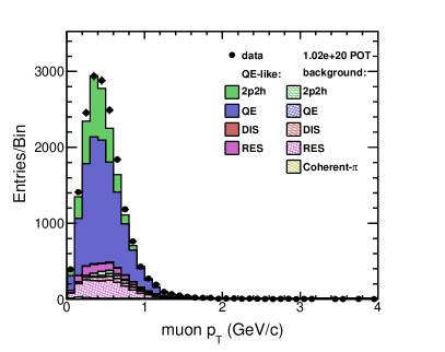
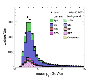
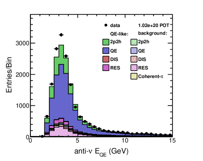
Figure 7: Distributions of signal and background events vs. muon transverse and longitudinal momentum, $Q^{2}_{QE}$ and $E_{\nu}^{QE}$ . Here the MINERvA-tuned GENIE simulation is absolutely normalized to the POT of the data sample, but the background corrections described in this section have not yet been applied. The $Q^{2}_{QE}$ distribution is shown on a log scale to highlight the high $Q^{2}_{QE}$ region. In the simulation, signal events include both quasi-elastic events (purple), 2p2h scatters (green) and resonant or DIS events (pink and red) with a QE-like signature. The backgrounds consist of quasi-elastic and 2p2h events with non-QE-like signature (hatched purple and green), and non-QE events (resonant and DIS) without a QE-like signature (hatched pink and red).

Backgrounds in this analysis arise primarily from events involving charged pions. MINERvA’s charged pion production analysis McGivern et al. (2016) suggests that GENIE 2.8.4 over-predicts the rate of resonant pion production. We therefore use a data-driven fitting procedure to constrain the backgrounds predicted by GENIE. Since the constraint can in principle be different in each $p_{T}/p_{\parallel}$ bin, the fit would ideally be done separately in each bin. However, the limited statistics of our data sample caused attempts to fit each bin separately to fail. The fits are instead performed separately for five regions of the $p_{T}/p_{\parallel}$ phase spaces, chosen by combining $p_{T}/p_{\parallel}$ bins with similar background shapes.

For each of the five regions, the recoil energy, after all other cuts, is compared for data, and for signal and background Monte Carlo. The TFractionFitter tool, part of the ROOT framework Brun and Rademakers (1997), is used to perform a fractional fit of the simulation to data, where the relative normalization of the signal and background distributions is allowed to vary. The shapes of the distributions are not varied.

Figure 8 shows the recoil distributions in data and (area-normalized) simulation for one of the five regions of $p_{T}/p_{\parallel}$, before and after tuning the signal and background fractions. In each bin, a scale is extracted corresponding to the factor by which the background fraction was rescaled relative to the nominal simulation to give the best fit. The estimated background fraction in each bin of the data distribution corresponds to the background fraction of the Monte Carlo in that bin, multiplied by this scale factor.

The scales for the $p_{T}$ vs. $p_{\parallel}$ regions are shown in Table 2. In most cases, as suggested by Eberly et al. (2015), the simulation is found to predict too high a fraction of background events.

Figure 8: Area normalized recoil distributions before (above) and after (below) background tuning for the bin corresponding to $0.25<p_{T}<0.4$ GeV. The blue boxes indicate the uncertainty in the simulation (red curve) estimated by TFractionFitter.

Bin	$p_{T}$ range	$p_{\parallel}$ range	background	background	$\chi^{2}$/dof.
	(GeV/c)	(GeV/c)	rescale factor	fraction
0	0.00 - 0.15	1.5 - 15	0.609$\pm$0.060	0.130$\pm$0.013	0.68
1	0.15 - 0.25	1.5 - 15	0.680$\pm$0.046	0.110$\pm$0.008	0.70
2	0.25 - 0.40	1.5 - 15	0.750$\pm$0.034	0.099$\pm$0.005	0.64
3	0.40 - 1.50	1.5 - 4.0	0.840$\pm$0.033	0.17$\pm$0.007	0.78
4	0.40 - 1.50	4.0 - 15	1.00$\pm$0.046	0.25$\pm$0.011	0.50

Table 2: Summary of the fits to determine the background fraction in data. The scale applied to the background to match the data, the resulting background fraction in the signal region and the $\chi^{2}$/DOF of the fit are shown.

Figure 9 shows the signal fraction as a function of the muon kinematic variables. After background subtraction, the signal data sample has estimated 14,839 events.

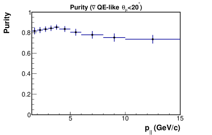
Figure 9: Purity (signal/total) as a function of kinematic variables.

Unfolding

Detector smearing is corrected using a migration matrix that describes the relationship between true and reconstructed bins of $p_{T}$ and $p_{\parallel}$. The migration matrix for our simulated reconstructed QE-like signal distribution is shown in Fig. 10. The $x$ axis indicates bins in the reconstructed variables, where the bins of $p_{\parallel}$ are repeated for each bin of $p_{T}$ . The $y$ axis indicates bins in the true variables, arranged in the same way. Thus any events on the diagonal were reconstructed in the correct bin of both $p_{\parallel}$ and $p_{T}$ . An event reconstructed in the wrong bin of $p_{\parallel}$ (but the right $p_{T}$ bin) will be displayed in another bin in the same subplot; one reconstructed in the wrong $p_{T}$ bin will appear in a different subplot.

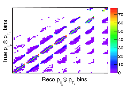
Figure 10: Migration matrix for the $p_{\parallel}$ $\otimes$$p_{T}$ distribution. The $x$ axis corresponds to reconstructed bins, the $y$ to true. The large cells correspond to $p_{T}$ bins while the small cells are the $p_{\parallel}$ bins within a $p_{T}$ bin. The high $p_{T}$ overflow bin is included.

We use the iterative method of D’Agostini D’Agostini (2010), as implemented in the ROOT package RooUnfold Adye (2011), with four iterations. The unfolding procedure was validated using an ensemble test, in which ten data-sized subsamples of the simulation were selected and warped by an adjustment of the quasi-elastic axial mass by $\pm 25$%. These samples were then unfolded using the migration matrix generated from the full un-warped simulation; the warped simulation was recovered within four iterations.

Efficiency and acceptance correction

The unfolded distributions are then corrected for detector acceptance and reconstruction efficiency. The most significant effect on acceptance is from the requirement that final-state muons are matched in MINOS, limiting the muon’s angle with respect to the beam line to a maximum of $20^{\circ}$. The MINOS-match requirement also limits our ability to accept muons with low longitudinal momentum $\lesssim 1.5$ GeV/c which will stop in MINERvA or not produce enough activity to be analyzed in the MINOS spectrometer. The largest source of inefficiency is due to the $Q^{2}_{QE}$ -dependent $E_{\text{recoil}}$ cut.

We estimate the product of acceptance and efficiency using the full MINERvA-tuned GENIE+Geant4 simulation:

$$\epsilon_{ij}=\frac{N_{ij}^{\text{generated and reconstructed}}}{N_{ij}^{\text{generated}}},$$ (10)

where ${N_{ij}^{\text{generated and reconstructed}}}$ is the number of simulated events generated in $p_{T}$ bin i and $p_{\parallel}$ bin j that also pass all reconstruction cuts (except the fiducial cuts on position and muon angle), and ${N_{ij}^{\text{generated}}}$ is the total number of events generated in $p_{T}$ bin $i$ and $p_{\parallel}$ bin $j$.

Figure 11 shows the product of efficiency and acceptance vs. $p_{\parallel}$ and $p_{T}$ . The low acceptance at high $p_{T}$ and low $p_{\parallel}$ is due to the MINOS match requirement and angle cut. The efficiency also decreases at higher energies, where interactions are more likely to include large amounts of recoil energy and may be vetoed by our $Q^{2}_{QE}$ -dependent $E_{\text{recoil}}$ cut. The overall efficiency $\times$ acceptance of the sample is 52.5%.

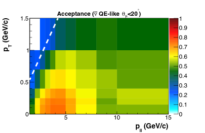
Figure 11: Efficiency $\times$ acceptance versus generated $p_{T}$ and $p_{\parallel}$ , for QE-like events in the simulation. The dashed white line illustrates the 20 degree limit imposed on reconstructed muon angles.

Flux and Target Number Correction

To convert an acceptance-corrected distribution to a cross section, we divide by the number of nucleons, the total number of protons on target (POT) producing the neutrino beam, and the estimated anti-neutrino flux per POT. These are summarized in Table 3.

Quantity	Value
Protons on target (data)	$1.020\times 10^{20}$
Protons on target (simulation)	$9.247\times 10^{20}$
Number of targets	$3.23478\times 10^{30}$ nucleons
Integrated flux	$2.340\times 10^{-8}\;\bar{\nu}_{\mu}/\text{cm}^{2}$ / POT

Table 3: Normalization factors used in the cross section calculations. The flux used in the quoted cross sections is integrated from 0-100 GeV.

The NuMI beam’s flux prediction is explained in detail in Aliaga Soplin (2016), and is summarized in section IV. For distributions in the $p_{T}$ /$p_{\parallel}$ phase space, we report flux-integrated cross sections. We do the same for the single-differential cross section $d\sigma/dQ^{2}_{QE}$. We integrate over the entire available flux range of 0-100 GeV, to get a total integrated flux of $2.295\times 10^{-8}$ cm^-2 per proton on target.

For the cross section as a function of $E_{\nu}^{QE}$ / $Q^{2}_{QE}$ , one can create an approximate flux-weighted cross section, where the number of events in each $E_{\nu}^{QE}$ bin is normalized by the flux in the corresponding $E_{\nu}$ bin. This is not a true total cross section, since $E_{\nu}^{QE}$ is not the true neutrino energy, except in the case of quasi-elastic scatters off of hydrogen. However $E_{\nu}^{QE}$ is closely correlated to $E_{\nu}^{true}$ (see Fig. 12), making the flux-weighted cross section a close approximation of the total cross section versus energy.

Figure 12: Ratio between the neutrino energy reconstructed from true muon kinematics and the true neutrino beam energy in the simulation. True quasi-elastic events show dispersion due to Fermi motion while 2p2h and resonance events tend to underestimate the true neutrino energy.

The target for an anti-neutrino quasi-elastic scatter (Eq. 1) is a proton. For QE-like scattering, it is possible that a scattering process could originate on a neutron (e.g. $\bar{\nu}_{\mu}n\to\mu^{+}\Delta^{-}$) where the resonance decays $\Delta^{-}\to n\pi^{-}$ and the pion is absorbed, or on a nucleon pair. We use the total number of nucleons in the fiducial volume as the target number normalization. The fiducial volume is made up of a combination of polystyrene, doping agents, epoxy and light-tight coating. The predominant material is polystyrene, which is composed of equal parts carbon and hydrogen. A full summary of the composition of the MINERvA tracker is available in Aliaga et al. (2014). We estimate that the fiducial volume used in this analysis contains $3.23\times 10^{30}$ nucleons, of which $1.76\times 10^{30}$ are protons.

VIII Systematic Uncertainties

Systematic uncertainties on the cross section measurements arise from many sources. To assess these systematic uncertainties, we vary parameters in the simulation within their uncertainties and recalculate the cross-sections using new estimates of efficiency, backgrounds, unsmearing, flux and target number corrections. The difference between this new cross section and the original result is taken to be the systematic uncertainty on the cross section due to that source. The sources of systematic uncertainty are discussed below. Systematic uncertainties in each category, and total systematic uncertainties, are available in Appendix XI.

Flux Uncertainties

The simulation of the NuMI flux and its uncertainties are described in detail in Aliaga et al. (2016). Uncertainties in the anti-neutrino flux arise primarily from uncertainties in hadron production rates and in parameters that control the alignment of the NuMI focusing system, such as the position of the focusing horns. These uncertainties are constrained with both external data and with a MINERvA measurement of elastic neutrino scattering on electrons Park et al. (2016). The total uncertainty in the focusing peak is approximately 8%, and rises to 11% at the falling edge of the focusing peak, where beam focusing uncertainties are large.

Parameter	Variation	% effect
Quasi-elastic axial mass (fixed normalization)	$\pm 15\%$	$<2\%$
Quasi-elastic normalization	$+20\%-15\%$	2-4%
Vector form factor model	BBBA05 $\rightarrow$ Dipole	$<1\%$
Pauli suppression	$30\%$	$<2\%$
NC Axial mass	$\pm 25\%$	$<0.5\%$
Strange axial form factor for NC	$\pm 30\%$	$<0.5\%$
NC resonance production rate	$\pm 20\%$	$<0.5\%$
Axial mass for resonance production	$\pm 20\%$	3-6%
Vector mass for resonance production	$\pm 3\%$	$<1\%$
Non-resonant 1-pion production rate ($\nu:n$ or $\bar{\nu}:p$)	$\pm 5\%$	$<0.5\%$
Non-resonant 2-pion production rate ($\nu:n$ or $\bar{\nu}:p$)	$\pm 50\%$	$<0.5\%$
Non-resonant 1-pion production rate ($\nu:p$ or $\bar{\nu}:n$)	$\pm 50\%$	$<0.5\%$
Non-resonant 2-pion production rate ($\nu:p$ or $\bar{\nu}:n$)	$\pm 50\%$	$<0.5\%$
Neutron mean free path	$\pm 20\%$	$1-5\%$
Pion mean free path	$\pm 20\%$	$<1\%$
Nucleon elastic scattering cross section	$\pm 30\%$	$<1\%$
Pion elastic scattering cross section	$\pm 10\%$	$<1\%$
Nucleon inelastic scattering cross section	$\pm 40\%$	$<1\%$
Pion inelastic scattering cross section	$\pm 40\%$	3-5%
Nucleon charge exchange cross section	$\pm 50\%$	$<1\%$
Pion charge exchange cross section	$\pm 50\%$	$<1\%$
Nucleon absorption cross section	$\pm 20\%$	$<2\%$
Pion absorption cross section	$\pm 20\%$	3-5%
Nucleon pion production cross section	$\pm 20\%$	$<1\%$
Pion pion production cross section	$\pm 20\%$	$<1\%$
DIS hadronization model adjustment	$\pm 20\%$	$<1\%$
Pion angle distribution (resonant events)	Isotropic $\to$ Rein-Sehgal	$<0.5\%$
Resonant decay photon branching ratio	$\pm 50\%$

Table 4: Summary of variable GENIE uncertainties

Parameter	Variation	% effect
RPA high $Q^{2}$	turn off relativistic effects	$<$ 1%
RPA low $Q^{2}$	estimate from muon capture	0-2%
2p2h np only	tune to 2p2h np only	$<$ 1%
2p2h pp only	tune to 2p2h pp only	0-2%
1p1h only	turn off 2p2h but tune 1p1h	0-5%

Table 5: Summary of uncertainties in the cross sections extracted using the MINERvA-tuned GENIE due to the 2p2h and RPA enhancements of default GENIE 2.8.4 model. Almost all bins have uncertainties of less than 2% with the largest effects only seen in the highest $p_{T}$ bins.

Muon Reconstruction Uncertainties

There are several uncertainties associated with reconstruction of the muon track, arising from uncertainties in the muon energy scale, tracking efficiencies, angular resolution and vertex reconstruction. The most significant of these is the muon energy scale uncertainty, which has contributions from several sources, including an 11 MeV uncertainty in energy loss from MINERvA’s material assay, a 30 MeV uncertainty in the energy deposition rate in MINERvA, $\frac{dE}{dx}$ and a momentum-dependent uncertainty for MINOS muon energy reconstruction Michael et al. (2008b). The MINOS uncertainty is 2% for muons whose momentum is measured by range, added in quadrature with either 0.6% for muons whose momentum is measured by curvature to be above 1GeV, or 2.5% for muons whose momentum is measured by curvature to be below 1GeV.

Muon tracking efficiencies in MINERvA and MINOS are measured by reconstructing tracks in one detector, extrapolating to the other detector, and observing the fraction of tracks matched in both detectors in data and in the simulation. The simulation is corrected for small discrepancies between tracking efficiencies, 0.5% $\pm$ 0.25% for MINERvA and 0.5 (2.5)% $\pm$ 0.25 (1.25)% for MINOS for muons with momentum greater than (less than) 3.0 GeV.

Potential angular reconstruction biases are estimated both by cutting tracks in half and comparing the reconstructed angles of both halves, as well as studies of forward-going events such as neutrino-electron scattering and low hadronic recoil events. These studies limit additional angular smearing or bias in the data relative to the simulation to below 1 milliradian.

Smearing of reconstruction vertices causes some events within the fiducial volume to be misreconstructed outside the fiducial volume, and visa versa. We estimate the uncertainty due to this effect by smearing reconstructed vertices in the simulation by 0.9 mm in x, 1.25 mm in y and 1 cm in z; this results in a negligible change in measured cross section.

The MINERvA tracker consists of primarily scintillator strips, with smaller portions of epoxy, tape, reflective coating and wavelength shifting fibers. The total uncertainty on the mass of the tracker is 1.4% Aliaga et al. (2014).

Model Uncertainties

Models used in the simulation include various parameters that carry uncertainties. These include uncertainties in signal, background and final state interaction models. Most of these are evaluated using the reweighting prescription and parameter uncertainties recommended by the GENIE collaboration Andreopoulos et al. (2015). These parameters are listed in Table 4, along with the amount by which they are varied and the approximate effect on the cross sections.

GENIE uncertainties that change particle fates cannot be modeled using the re-weighting method. In this case, we generate an alternative simulated sample in which these parameters, including the effective nuclear radius, formation zone and hadronization model, have been adjusted.

The RPA correction described in section IV is applied when calculating the central values. The correction is varied within the uncertainties shown in figure 2. Similarly, the addition of the 2p2h process is estimated by adding events from correlated pairs as described in section IV and reference Gran et al. (2013). The uncertainty on this is determined by using several variations of the tuning procedure, including fits that allow interactions on $pp$ pairs, $np$ pairs, or single nucleon interactions to be tuned. The differences in cross-section obtained using these three variants from the standard simulation are added in quadrature as a systematic error due to the 2p2h model. Table 5 summarizes the effects of these variations on the extracted cross sections.

Recoil reconstruction uncertainties

Several sources of uncertainties can affect the reconstruction of recoil energy, which can in turn change the background estimates and efficiencies used to estimate the cross sections. Quasi-elastic anti-neutrino events have a hadronic final state consisting of a neutron. In order for neutrons to deposit recoil energy in the detector, they must undergo an interaction, with resulting charged particles (usually protons) then depositing visible energy. The most significant source of uncertainty associated with neutrons is due to the Geant4 neutron interaction model. To evaluate this uncertainty, we vary the mean free path of neutrons in the detector, with the variations spanning discrepancies between Geant4 and thin target neutron scattering data on copper, iron and carbon Abfalterer et al. (2001); Schimmerling et al. (1973); Voss and Wilson (1956); Slypen et al. (1995); Franz et al. (1990); Tippawan et al. (2009); Bevilacqua et al. (2013); Zanelli et al. (1981).

Energy response of protons has been measured in the MINERvA test beam detector Aliaga et al. (2015). To propagate uncertainties on this measurement to the cross sections, we shift simulated recoil energy deposited by protons by uncertainties derived from comparisons of the test beam measurements and Geant4. The variation depends on the proton energy: 4% below 50 MeV and 3.5% above 50 MeV. The proton response affects our event rate measurement by less than $1\%$ across our whole phase space, as the track cut removes many protons, and only a small amount of those that remain pass into our selected sample by making this shift.

The pion calorimetric response has also been constrained by test beam studies to an accuracy of 4%, for pions with a kinetic energy between 400 and 1900 MeV. We thus separate our pions into two categories - “constrained” within this energy range, and “unconstrained” outside of it. Pions within the constrained range have their energy fraction varied by $\pm 4\%$, while others have it varied by $\pm 5\%$. The pion response has only a minor effect ($<1\%$ across our whole phase space) on our cross sections.

For the other particles (electromagnetic and kaons), we vary the recoil by $\pm 3\%$. This uncertainty was derived by observing the energy response for Michel electrons (electrons from muon decay), which have a well-known energy spectrum. This change mainly affects the $Q^{2}$ (${p_{T}}$) shape, and contributes its maximum of around 1% uncertainty at low $Q^{2}$.

These uncertainties are dominated by neutron interaction modeling, which ranges from 2-6%; the other uncertainties are less than 1%.

IX Results

Double-differential cross sections vs. $p_{T}$ and $p_{\parallel}$ are shown in Fig. 13. Double-differential cross sections vs. $E_{\nu}^{QE}$ ($E_{\nu}^{true}$ ) and $Q^{2}_{QE}$ are shown in Fig. 14 (Fig. 15). In each case, simulated cross sections are also plotted, where the simulation uses the MINERvA-tuned GENIE model described in IV. Results corrected to a quasi-elastic, rather than QE-like, signal definition are available in Appendix XII.

The MINERvA-tuned GENIE model agrees well with MINERvA data, in spite of the fact that the tune was made to an independent (neutrino rather than antineutrino) dataset. In the following sections, we compare these results with many alternate models and discuss the impact of the individual components of the MINERvA tune.

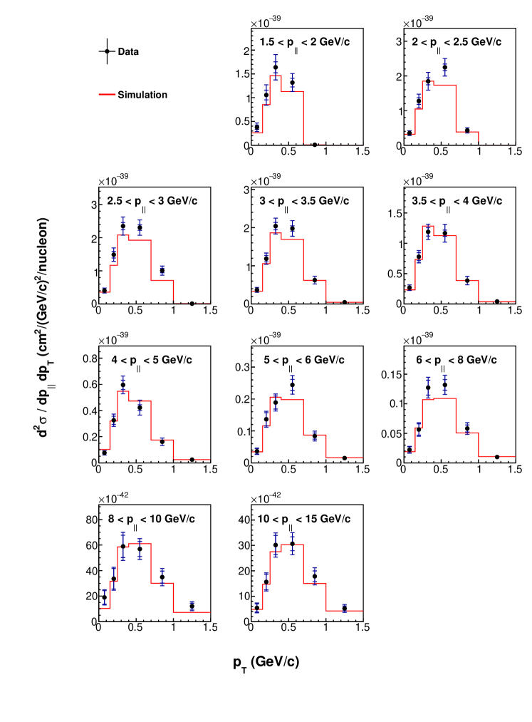
Figure 13: Double-differential QE-like cross section vs. muon transverse momentum, in bins of muon longitudinal momentum. Inner error bars show statistical uncertainties; outer error bars show total (statistical and systematic) uncertainty. The red histogram shows the MINERvA-tuned GENIE 2.8.4 model used to estimate smearing and acceptance. These results are tabulated in Tables 7–9.

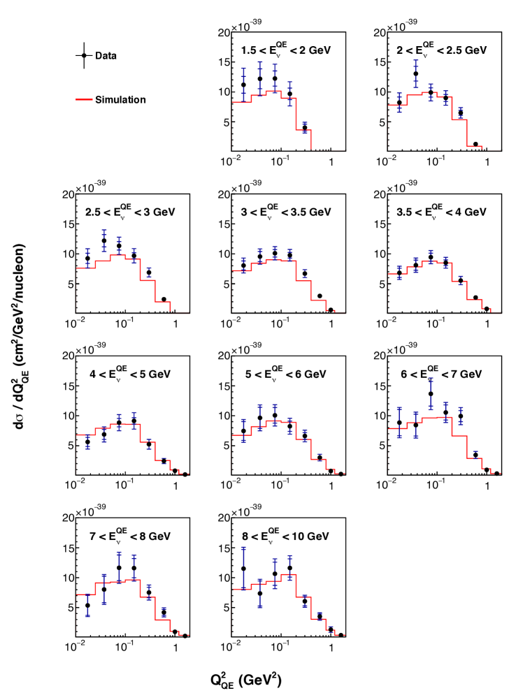
Figure 14: Differential QE-like cross section $d\sigma(E^{QE}_{\nu})/dQ^{2}_{QE}$, in bins of $E^{QE}_{\nu}$. Inner error bars show statistical uncertainties; outer error bars show total (statistical and systematic) uncertainty. The red histogram shows the MINERvA-tuned GENIE model used to estimate smearing and acceptance. These results are tabulated in Tables 12–14.

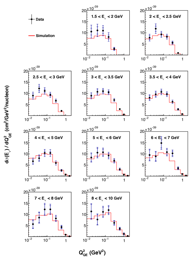
Figure 15: Differential QE-like cross section $d\sigma(E^{true}_{\nu})/dQ^{2}_{QE}$, in bins of $E^{true}_{\nu}$. The red histogram shows the MINERvA-tuned GENIE model used to estimate smearing and acceptance. These results are tabulated in Tables 17–19.

Figure 16 shows the data and the different components included in the MnvGENIE model. Events generated as pure 1p1h CCQE are shown in green, the resonance (and a small DIS) component is added to make the blue histogram. The addition of tuned 2p2h yields the red MnvGENIE curve. RPA corrections are applied to all three.

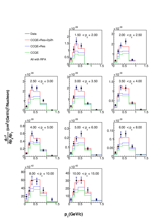
Figure 16: Double-differential QE-like cross section vs. muon transverse momentum, in bins of muon longitudinal momentum. Inner error bars show statistical uncertainties; outer error bars show total (statistical and systematic) uncertainty. The red histogram shows the MINERvA-tuned GENIE 2.8.4 model used to estimate smearing and acceptance which is CCQE + resonant + 2p2h. The green histogram shows events produced as CCQE, the blue curve shows default GENIE which is CCQE + resonant. These results are tabulated in Tables 7–9 and the models are included in the supplementary material.

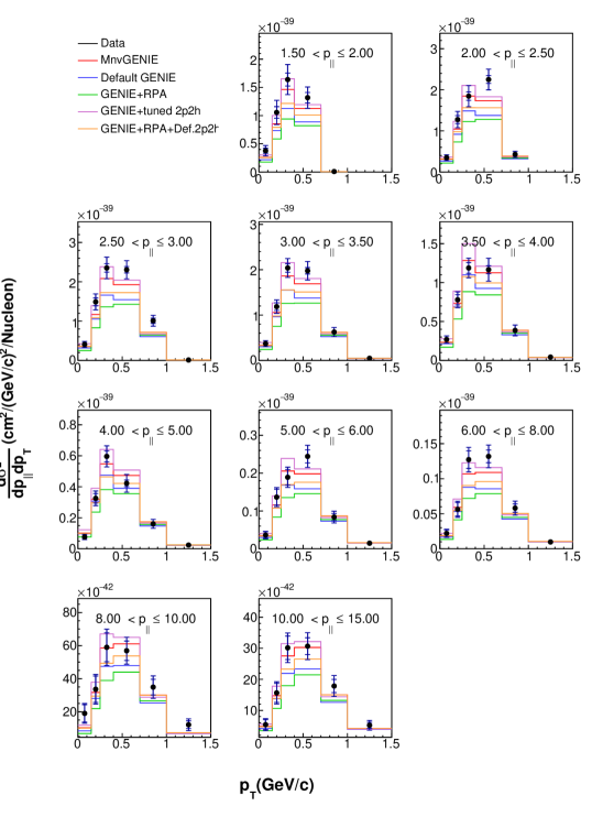
Figure 17: Double-differential QE-like cross section vs. muon transverse momentum, in bins of muon longitudinal momentum (black circles) compared to MINERvA-tuned GENIE (red curve, includes RPA and MINERvA-tuned 2p2h), GENIE without any modifications except the single non-resonant pion correction discussed in section IV (blue), GENIE with the RPA weight but no 2p2h component (green), GENIE with MINERvA-tuned 2p2h but no RPA (violet), and GENIE with RPA and untuned 2p2h (orange). Inner error bars show statistical uncertainties; outer error bars show total (statistical and systematic) uncertainty.

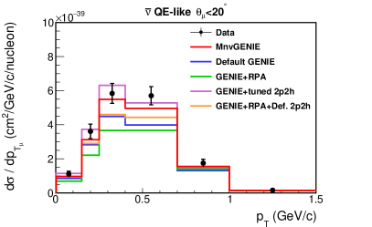
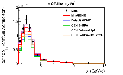
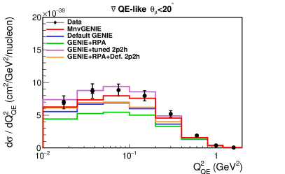
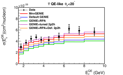
Figure 18: Single-differential projections of the double-differential QE-like cross section measurements compared to MINERvA-tuned GENIE (red curve, includes RPA and MINERvA-tuned 2p2h), GENIE without any modifications except the single non-resonant pion correction discussed in section IV (blue), GENIE with the RPA weight but no 2p2h component (green), GENIE with MINERvA-tuned 2p2h but no RPA (violet), and GENIE with RPA and untuned 2p2h (orange). Inner error bars show statistical uncertainties; outer error bars show total (statistical and systematic) uncertainty. These results are tabulated in Tables 10, 11, 15 and 16.

Figure 19: Ratio of the double-differential QE-like cross sections vs. muon transverse momentum shown in the previous figure, in bins of muon longitudinal momentum. In all cases, the denominator for the ratio is MINERvA-tuned GENIE (includes RPA and MINERvA-tuned 2p2h); the numerators are our measured cross section (black circles) , MINERvA-tuned GENIE (red), GENIE without any modifications (blue), GENIE with the RPA weight but no 2p2h component (green), GENIE with MINERvA-tuned 2p2h but no RPA (violet), and GENIE with RPA and untuned 2p2h (orange). Inner error bars show statistical uncertainties; outer error bars show total (statistical and systematic) uncertainty.

Comparisons to Alternate GENIE Models

Figure 17 shows the measured differential cross sections and several variations on the GENIE model; Single differential projections versus $p_{T}$, $p_{\parallel}$, $E_{\nu}^{QE}$, and $Q^{2}_{QE}$ are shown in Fig. 18 for the same variations.

In particular, the MINERvA-tuned GENIE (MnvGENIE in figures) model is GENIE with RPA and MINERvA-tuned 2p2h effects added. Other permutations of RPA, 2p2h and MINERvA-tuned 2p2h are also shown. Figure 19 shows the ratio of the measured differential cross section to the MINERvA-tuned GENIE model. Table 6 shows the $\chi^{2}$ for 58 degrees of freedom for the models shown in that figure and for additional theoretical models described in Section IX.

A standard $\chi^{2}$ comparison for these models relative to the data using the statistical uncertainties derived from the data gives a best agreement (the green curve with RPA but no 2p2h contribution) with the curve that lies furthest away from the data. This is due to the dominance of multiplicative normalization uncertainties in the covariance matrix, which leads to the well known pathology of Peelle’s Pertinent PuzzlePeelle (1987); Box and Cox (1964). This effect is well documented in the nuclear cross section literature Carlson et al. (2007) and, in the limit of pure multiplicative uncertainties, a $\chi^{2}$ derived from the log of the cross section is preferred to one derived from the cross section itself, since in the former case the multiplicative factors are normally distributed.

In addition, the $\chi^{2}$ statistic is known to have biases when uncertainties estimated from the counting statistics of individual data points are used. For statistical uncertainties estimated to be proportional to $\sqrt{N_{i}}$, points that fluctuate downwards are given smaller estimated uncertainties and hence greater weight in the $\chi^{2}$ calculation. For normalization uncertainties, the effect is even greater with the uncertainty being directly proportional to $N_{i}$. The normalization uncertainties in these data are highly correlated from bin to bin and substantial relative to the other uncertainties. For this reason, we report the $\chi^{2}$ using both the cross section itself (linear) and the log of the cross section (log-normal) in Table 6 in the next section. The lowest log-normal $\chi^{2}$ is for the MINERvA-tuned GENIE model with default 2p2h and the RPA correction which appears as the orange curve in Fig. 18, 17 and 19.

Comparisons to NuWro Models

We have also compared the data to several models available in the NuWro event generator. Table 6 summarizes the agreement between the data and these models while figures 20 and 22 show the comparisons. NuWro also includes models of 2p2h and RPA, and additionally includes an implementation of the Transverse Enhancement Model describe in Section II. The Relativistic Fermi Gas nuclear model is labeled GFG (Global Fermi Gas) to distinguish it from an alternate LFG (Local Fermi Gas) nuclear model. A Spectral Function model is also available in NuWro and included in the comparisons.

All of the NuWro models have higher $\chi^{2}$ values than the MINERvA-tuned GENIE model. Even when comparing very similar primary interaction models (e.g. default GENIE and NuWro GFG without RPA or 2p2h) between the two generators, the agreement with data is quite different. We believe this is due to the different FSI models used by NuWro and GENIE, which impact the predicted contribution to the cross section from events that include a pion that is absorbed before exiting the primary nucleus. Of the NuWro models, the preferred model includes RPA and 2p2h contributions, as is also the case with GENIE variants described above.

Model	conventional $\chi^{2}$	Log-Normal $\chi^{2}$
GENIE+def. 2p2h+RPA	70.4	96.5
MINERvA tuned GENIE	81.2	98.4
GENIE+RPA	66.1	117.9
Untuned GENIE	80.6	131.0
GENIE+2p2h	149.7	154.1
NuWro GFG+2p2h+RPA	72.4	105.0
NuWro LFG	85.4	111.3
NuWro GFG+TEM	86.9	113.7
NuWro GFG+TEM+RPA	80.9	125.7
NuWro GFG	108.4	177.5
NuWro Spectral Function	94.8	184.6
NuWro GFG+2p2h	153.7	185.9

Table 6: This table summarizes the $\chi^{2}$ values for comparisons of the differential cross section $d\sigma^{2}/dp_{T}dp_{\parallel}$ to a wide variety of models. The top 5 are GENIE variations illustrated in Fig. 17 while the bottom 7 are variations of the NuWro event generator illustrated in Figs. 20 and 21. The MINERvA-tuned GENIE model includes RPA and MINERvA-tuned 2p2h and was used in the extraction of the cross section. The $\chi^{2}$ is for 58 degrees of freedom.

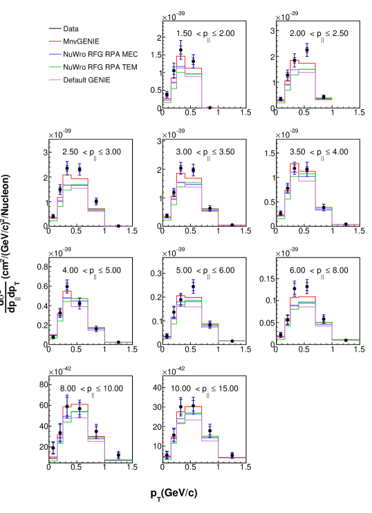
Figure 20: Double-differential QE-like cross section vs. muon transverse momentum, in bins of muon longitudinal momentum compared to the MINERvA-tuned GENIE (red curve), the NuWro Nieves RFG model with Random Phase Approximation and Meson Exchange current (MEC) (blue curve) and the NuWro Relativistic Fermi Gas RFG model with RPA and Transverse Enhancement added (green curve). Inner error bars show statistical uncertainties; outer error bars show total (statistical and systematic) uncertainty.

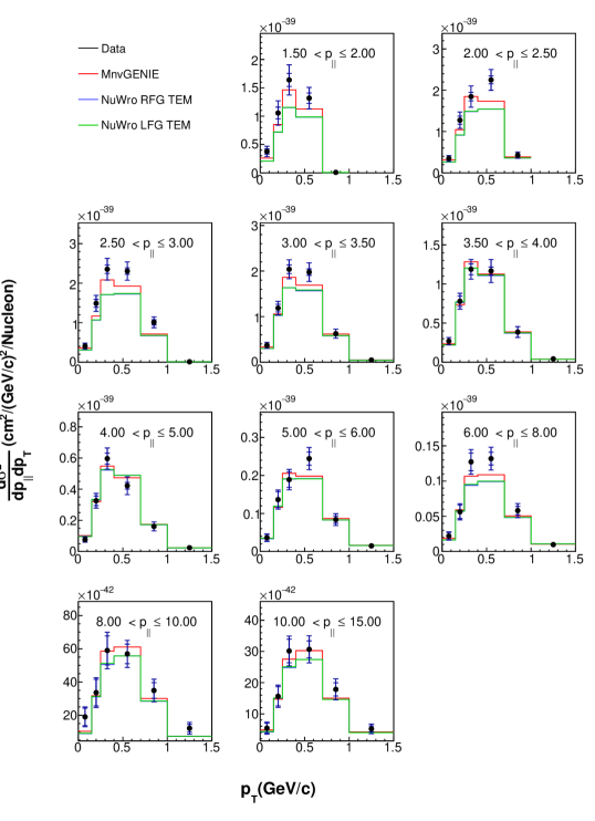
Figure 21: Double-differential QE-like cross section vs. muon transverse momentum, in bins of muon longitudinal momentum compared to the MINERvA-tuned GENIE (red curve) and the NuWro Relativistic (RFG) Fermi Gas model with Transverse Enhancement (RFG+TEM, blue curve) and the NuWro Local Fermi Gas (LFG) model with Transverse Enhancement (LFG+TEM, green curve). Inner error bars show statistical uncertainties; outer error bars show total (statistical and systematic) uncertainty.

Figure 22: Double-differential QE-like cross section vs. muon transverse momentum, in bins of muon longitudinal momentum compared to the MINERvA-tuned GENIE (red curve), NuWro and GENIE RFG implementations (blue and purple) and the NuWro Spectral Function model (green curve). Inner error bars show statistical uncertainties; outer error bars show total (statistical and systematic) uncertainty.

Comparisons to other experiments

Figs 23 and 24 show the cross sections versus $E_{\nu}^{QE}$ , corrected to cross section/proton, compared to results from MiniBooNE Aguilar-Arevalo et al. (2013) and NOMAD Lyubushkin et al. (2009). The MiniBooNE cross sections quoted are the average of their reported cross sections on mineral oil and their estimated rates on pure carbon, as our scintillator target lies approximately halfway between those two compositions. NOMAD is only shown for the true-QE assumption as they only quote results for that process. We note that the caveats discussed in section VII should be taken into account when comparing these results to other experiments – namely that this is an approximation of the energy dependent cross section, and that the approximations will have different impact on these results than those measured in beams with different neutrino energy spectra. Although the MINERvA data points show a small dip in the $\sim 4-6$ GeV region, they are consistent within uncertainties with models that predict a smoothly rising cross section in this region (see Fig. 18). The MINERvA neutrino flux Aliaga et al. (2016) changes rapidly in the 4-6 GeV region with uncertainties that are dominated by the neutrino beam focusing system (see the distribution of uncertainties vs $E_{QE}$ in Fig. 26 of Appendix XI).

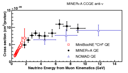
Figure 23: MINERvA true CCQE cross section as a function of $E_{\nu}^{QE}$ compared to data from the MiniBooNE and NOMAD experiments. Error bars show total (statistical and systematic) uncertainty.

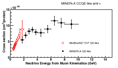
Figure 24: MINERvA QE-like cross section as a function of $E_{\nu}^{QE}$ compared to data from the MiniBooNE experiment. The MiniBooNE QE-like definition does not exclude events with proton KE $>$ 120 MeV as MINERvA does so the comparison is not exact. Error bars show total (statistical and systematic) uncertainty.

Vertex Energy Distributions

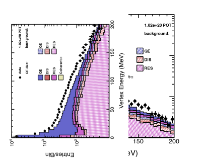
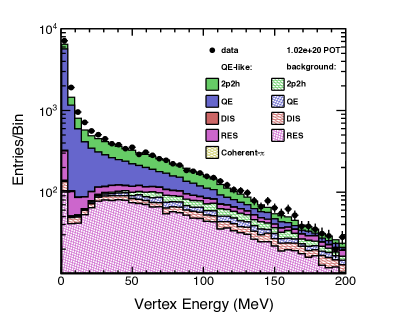
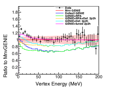
Figure 25: Reconstructed energy within 100 mm of the neutrino interaction vertex. The black points show MINERvA data. In the top plot, the stacked histograms show the predictions of various models using default GENIE 2.8.4. In the middle plot, the stacked histograms are for the MINERvA-tuned GENIE 2.8.4, which includes RPA and MINERvA-tuned 2p2h. The bottom plot shows the ratio of the data and various models to MINERvA-tuned GENIE. Statistical uncertainties only.

Because interactions on multi-nucleon pairs are expected to include additional low-energy nucleons compared to standard QE interactions, reconstructed energy near the interaction vertex is useful for judging the efficacy of 2p2h models. Figure 25 shows energy reconstructed in scintillator strips that are within 100 mm of the interaction vertex, in the sample used to produce the cross sections discussed earlier, but before background subtraction and efficiency, flux and target number corrections. Also shown are the expected distributions for default and MINERvA-tuned GENIE, and ratios to MINERvA-tuned GENIE for the data and several GENIE variants. Models that omit a 2p2h component have very poor agreement with the data, but the case for RPA suppression is not as strong. The model that lies closest to the data is the MINERvA-tuned GENIE with the RPA correction omitted. This is in conflict with similar conclusions drawn from cross-sections versus kinematic distributions, indicating that while MINERvA-tuned GENIE is a definite improvement over default GENIE 2.8.4, more improvements are needed to properly simulate the hadronic component of anti-neutrino QE-like interactions.

X Conclusion

We have presented a measurement of a QE-like cross section for anti-neutrino scattering on scintillator. The signal definition requires no charged pions in the final state and no protons with kinetic energies above 120 MeV. This variant of the QE-like definition allows us to include quasi-elastic scatters off of NN pairs in the nucleus in our signal definition and closely matches the actual sensitivity of our detector to low energy protons.

The main result is presented as a function of muon kinematics $p_{T}$ and $p_{\parallel}$. We also present an energy-dependent flux normalized cross section in terms of the neutrino energy and 4-momentum transfer squared as calculated from the muon kinematics using a quasi-elastic assumption. These data are compared to a large number of models for anti-neutrino QE-like scattering. In particular, we have applied corrections to the default GENIE 2.8.4 scattering model for the Random Phase Approximation and have added 2p2h processes that have been tuned to the observed recoil distributions in an independent MINERvA neutrino scattering sample. This MINERvA-tuned model agrees better with our data than default GENIE both visually (Fig. 19) and when a log-normal $\chi^{2}$ is calculated, as is more appropriate when multiplicative uncertainties are significant. Moreover, comparisons of reconstructed energy near the interaction vertex between these data and various models indicates poor agreement with models that do not include 2p2h.

In conclusion, addition of RPA and 2p2h effects to the simulation substantially improves agreement with the MINERvA QE-like data over default GENIE. Addition of either RPA or 2p2h alone is not sufficient. However, substantial discrepancies between the improved model and data remain, indicating that more model development is needed. This is the first double-differential measurement of quasi-elastic or QE-like scattering cross sections for anti-neutrinos in this energy range, which is very similar to the expected spectrum of the DUNE experiment, and will be an essential component in the development and tuning of models used in future neutrino oscillation measurements.

XI Appendix: Summary of Systematic Uncertainties

Figure 26 shows a summary of the fractional systematic uncertainties from each of category of uncertainty described in section VIII for the one dimensional cross-sections. The model uncertainties have been further subdivided into those primarily affecting the signal models (quasi-elastic and 2p2h), background models, and final state interactions. Figures 27 and 28 show fractional uncertainties on the double-differential cross sections. Figure 29 shows the correlation matrix for all systematic uncertainties.

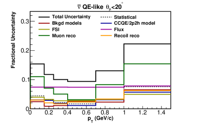
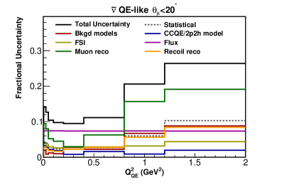
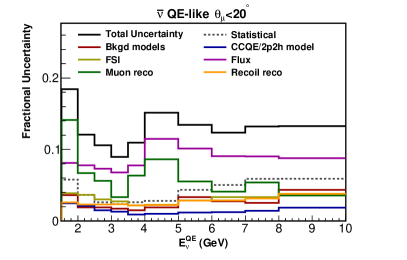
Figure 26: Summary of fractional uncertainties on the single-differential projections of the double-differential QE-like cross section measurements in data. The cross sections themselves are shown in Fig. 18.

Figure 27: Absolute fractional uncertainties on the double-differential QE-like cross section vs. muon transverse momentum, in bins of muon longitudinal momentum.

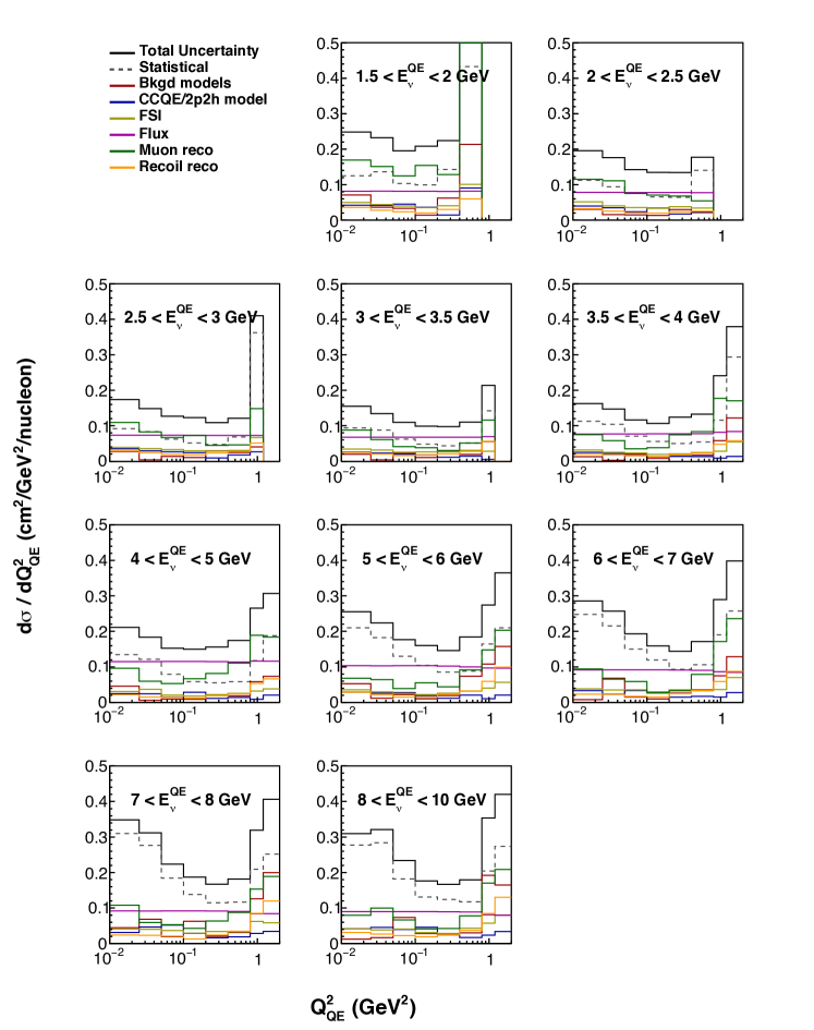
Figure 28: Absolute fractional uncertainties on the cross section vs. $Q^{2}$, in bins of $E_{\nu}^{QE}$ .

Figure 29: Correlation matrix for the 6$\times$ 10 $p_{T}$ and $p_{\parallel}$ bins. As in the migration matrix, the larger blocks are $p_{T}$ bins with the smaller scale bins $p_{\parallel}$ bins.

XII Appendix: CCQE Cross-Sections

The main focus of the analysis was the calculation of CCQE-like double-differential cross sections shown above, which correspond to our measurement for the signal definition described in section VI. As an extension to the analysis, however, we also calculated a true CCQE cross section. Recall that, for the CCQE-like cross section, our signal corresponded to interactions with a CCQE-like final state, even if that final state was generated by a resonant or DIS interaction followed by FSI. For the true CCQE definition, our signal corresponds only to events where the initial interaction was quasi-elastic, even if FSI created final-state particles such as pions that mimicked a non-quasi-elastic interaction. The signal also includes 2p2h events where a CCQE interaction takes place on a correlated pair.

The true CCQE double-differential cross sections are shown in Fig. 30 ($d^{2}\sigma/dp_{T}dp_{\parallel}$) and 31 ($d\sigma(E_{\nu}^{QE})/dQ^{2}_{QE}$), while one-dimensional projections are shown in Fig. 32. Also shown in these figures are the predictions in our default simulation, which includes both CCQE and 2p2h contributions.

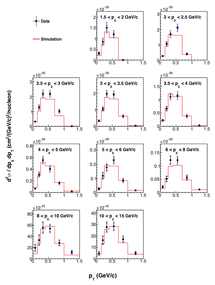
Figure 30: Double-differential flux-integrated true CCQE cross section $d^{2}\sigma/dp_{T}dp_{\parallel}$ vs. muon transverse momentum, in bins of muon longitudinal momentum. Inner error bars show statistical uncertainties; outer error bars show total (statistical and systematic) uncertainty. These results are tabulated in Tables 22–24.

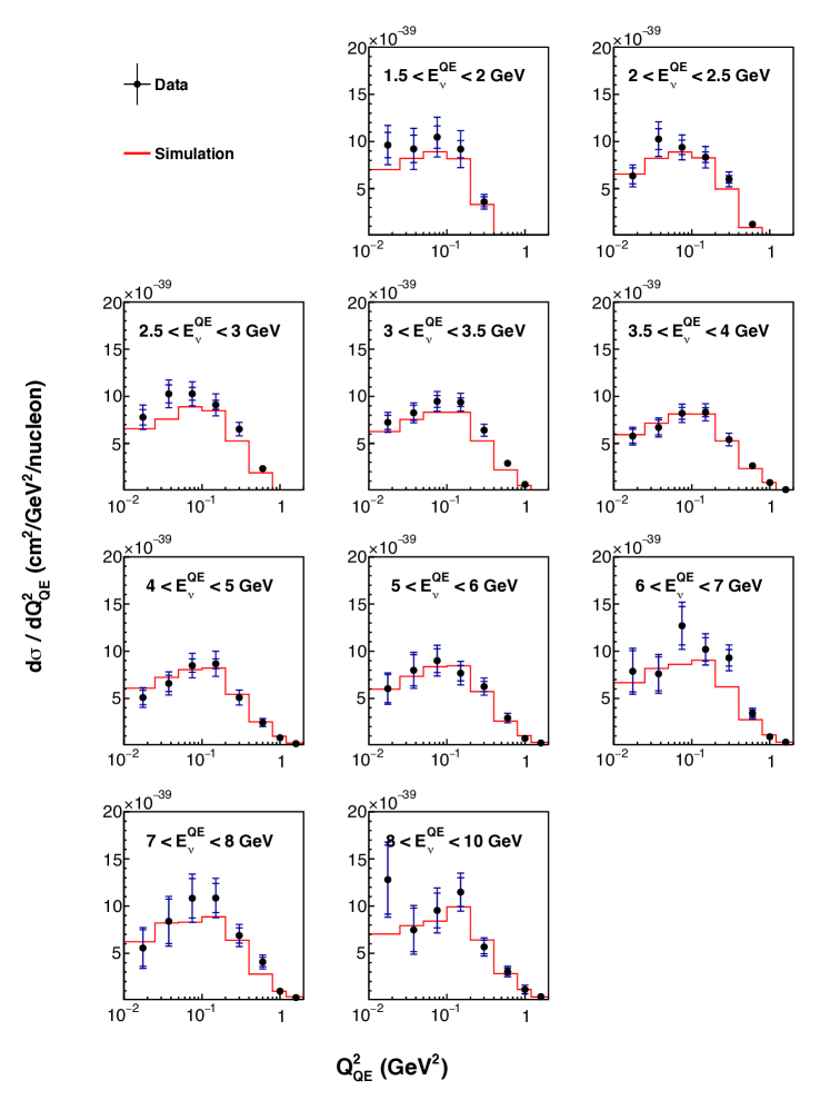
Figure 31: True CCQE cross section $d\sigma(E_{\nu}^{QE})/dQ^{2}_{QE}$, in bins of $E_{\nu}^{QE}$. Inner error bars show statistical uncertainties; outer error bars show total (statistical and systematic) uncertainty. These results are tabulated in Tables 27–29.

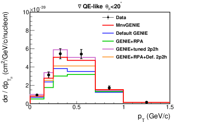
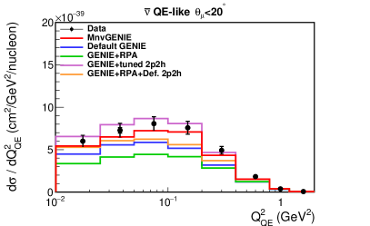
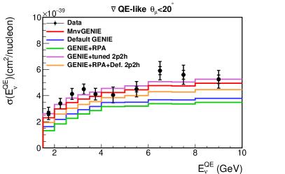
Figure 32: Single-differential projections of the double-differential true CCQE cross section measurements in data, compared to MINERvA-tuned GENIE (red curve, includes RPA and MINERvA-tuned 2p2h), GENIE without any modifications except the single non-resonant pion correction discussed in section IV (blue), GENIE with the RPA weight but no 2p2h component (green), GENIE with MINERvA-tuned 2p2h but no RPA (violet), and GENIE with RPA and untuned 2p2h (orange). Inner error bars show statistical uncertainties; outer error bars show total (statistical and systematic) uncertainty. These results are tabulated in Tables 25, 26, 30 and 31.

XIII Appendix: Tables of cross section measurements

CCQE-like cross sections

The tables in this section list our cross section measurements for the CCQE-like signal definition explained in section VI. For all of the double-differential measurements, we show a table of values corresponding to the cross section, followed by a table of statistical uncertainties, then a table of systematic uncertainties. Units are explained in the captions to the tables.

$p_{T}$ and $p_{\parallel}$ 

The differential cross section with respect to muon parallel and transverse momentum, $d^{2}\sigma/dp_{T}dp_{\parallel}$ is shown in Table 7. The statistical uncertainty on these measurements are shown in Table 8, and the systematic uncertainty in Table 9.

Table 10 shows the differential cross section $d\sigma/dp_{T}$, generated by projecting the two-dimensional measurement onto the $p_{T}$ axis. Table 11 shows the differential cross section $d\sigma/dp_{\parallel}$, generated by projecting the two-dimensional measurement onto the $p_{\parallel}$ axis. Both tables also include statistical and systematic uncertainties.

	0-0.15	0.15-0.25	0.25-0.4	0.4- 0.7	0.7-1	1-1.5
1.5 - 2	37.71	105.56	163.89	131.76	0.84	0.00
2 - 2.5	34.86	127.51	184.54	224.95	42.85	0.00
2.5 - 3	40.67	148.90	235.21	230.56	100.81	1.10
3 - 3.5	37.01	118.56	203.85	197.59	62.56	4.63
3.5 - 4	26.85	77.89	118.78	116.54	38.53	4.22
4 - 5	7.64	32.55	59.60	42.21	16.10	2.43
5 - 6	3.63	13.65	18.91	24.43	8.39	1.48
6 - 8	2.20	5.64	12.73	13.19	5.81	0.98
8 - 10	1.90	3.36	5.89	5.69	3.49	1.21
10 - 15	0.54	1.56	3.01	3.07	1.78	0.52

Table 7: Measured double-differential CCQE-like cross section $d^{2}\sigma/dp_{T}dp_{\parallel}$. Units are $10^{-41}$cm²/GeV²/nucleon. Columns represent bins of $p_{T}$ (GeV), rows are bins of $p_{\parallel}$ (GeV).

	0-0.15	0.15-0.25	0.25-0.4	0.4- 0.7	0.7-1	1-1.5
1.5 - 2	4.58	10.27	11.49	9.18	0.39	0.00
2 - 2.5	4.02	9.62	10.17	9.43	5.05	0.00
2.5 - 3	4.09	9.97	10.77	8.27	6.62	0.40
3 - 3.5	3.76	8.43	9.50	7.02	4.30	1.12
3.5 - 4	3.12	6.58	6.89	5.09	3.06	0.93
4 - 5	1.16	3.09	3.54	2.16	1.37	0.44
5 - 6	0.88	2.09	2.05	1.73	0.96	0.32
6 - 8	0.51	0.96	1.26	0.90	0.60	0.18
8 - 10	0.53	0.80	0.87	0.59	0.47	0.23
10 - 15	0.16	0.31	0.38	0.27	0.21	0.10

Table 8: Statistical uncertainty on the measured double-differential CCQE-like cross section $d^{2}\sigma/dp_{T}dp_{\parallel}$. Units are $10^{-41}$cm²/GeV²/nucleon. Columns represent bins of $p_{T}$ (GeV), rows are bins of $p_{\parallel}$ (GeV).

	0-0.15	0.15-0.25	0.25-0.4	0.4- 0.7	0.7-1	1-1.5
1.5 - 2	6.32	17.38	23.03	15.69	0.36	0.00
2 - 2.5	4.17	15.24	22.51	22.07	5.01	0.00
2.5 - 3	4.70	15.92	23.89	20.42	10.60	0.24
3 - 3.5	3.95	10.85	17.21	18.32	8.45	1.04
3.5 - 4	2.61	6.72	10.14	13.55	5.96	0.89
4 - 5	0.97	3.28	5.60	5.26	2.49	0.53
5 - 6	0.39	1.21	1.64	2.36	1.21	0.35
6 - 8	0.22	0.55	1.14	1.35	0.80	0.21
8 - 10	0.22	0.34	0.63	0.56	0.49	0.27
10 - 15	0.09	0.15	0.27	0.34	0.26	0.12

Table 9: Systematic uncertainty on the measured double-differential CCQE-like cross section $d^{2}\sigma/dp_{T}dp_{\parallel}$. Units are $10^{-41}$cm²/GeV²/nucleon. Columns represent bins of $p_{T}$ (GeV), rows are bins of $p_{\parallel}$ (GeV).

Bin	Cross	Statistical	Systematic
	section	uncertainty	uncertainty
0 - 0.15	110.74	4.93	16.30
0.15 - 0.25	361.23	11.20	41.01
0.25 - 0.4	583.94	12.33	57.20
0.4 - 0.7	570.42	9.66	52.65
0.7 - 1	174.81	5.53	22.10
1 - 1.5	15.87	1.20	3.32

Table 10: Differential CCQE-like cross section $d\sigma/dp_{T}$, along with statistical and systematic uncertainties. Units are $10^{-41}$cm²/GeV/nucleon. The $p_{T}$ bins are in GeV.

Bin	Cross	Statistical	Systematic
	section	uncertainty	uncertainty
1.5 - 2	80.58	3.48	11.25
2 - 2.5	126.00	3.73	13.98
2.5 - 3	156.23	3.76	15.40
3 - 3.5	128.35	3.08	12.41
3.5 - 4	78.27	2.26	8.66
4 - 5	32.05	1.02	3.73
5 - 6	15.33	0.73	1.53
6 - 8	8.99	0.40	0.92
8 - 10	4.86	0.31	0.52
10 - 15	2.40	0.13	0.28

Table 11: Differential CCQE-like cross section $d\sigma/dp_{\parallel}$, along with statistical and systematic uncertainties. Units are $10^{-41}$cm²/GeV/nucleon. The $p_{\parallel}$ bins are in GeV.

$E_{\nu}^{QE}$ and $Q^{2}_{QE}$

The reconstructed energy-dependent cross section vs $Q^{2}_{QE}$, $d\sigma(E_{\nu}^{QE})/dQ^{2}_{QE}$ is shown in Table 12. The statistical uncertainty on these measurements is in Table 13, and the systematic uncertainty in Table 14.

The total reconstructed energy-dependent cross section $\sigma(E_{\nu}^{QE})$, generated by dividing the event count $N_{i}(E_{\nu}^{QE})$ in each bin by that energy bin’s flux $\Phi(E_{\nu})$, is shown in Table 15. Note that $E_{\nu}^{QE}$ is the neutrino energy reconstructed using muon kinematics assuming a quasi-elastic hypothesis and is different than true the true incoming neutrino energy $E_{\nu}^{true}$ . The differential cross section with respect to reconstructed $Q^{2}_{QE}$, $d\sigma/dQ^{2}_{QE}$, is shown in Table 16. Tables 15 and 16 also include statistical and systematic uncertainties.

	0.0-0.025	0.025-0.05	0.05-0.1	0.1-0.2	0.2-0.4	0.4-0.8	0.8-1.2	1.2-2
1.5 - 2	1118.91	1219.53	1224.29	968.17	404.04	1.08	0.00	0.00
2 - 2.5	823.22	1304.80	991.07	899.36	650.50	129.16	0.00	0.00
2.5 - 3	924.55	1219.48	1134.01	968.24	688.89	241.79	4.44	0.00
3 - 3.5	805.21	954.82	1009.61	976.76	670.47	296.84	63.60	0.00
3.5 - 4	682.27	810.94	944.45	851.43	553.80	270.56	81.75	8.34
4 - 5	562.66	688.42	884.91	914.05	524.28	244.33	81.80	18.68
5 - 6	746.09	964.90	1006.93	824.64	662.22	301.57	77.13	26.32
6 - 7	885.65	844.16	1366.60	1055.01	994.06	344.99	96.90	34.75
7 - 8	536.48	802.64	1164.94	1159.34	752.25	420.73	96.69	25.83
8 - 10	1151.00	736.27	1064.92	1161.83	605.77	351.78	132.23	39.22

Table 12: Measured reconstructed energy-dependent CCQE-like cross section $d\sigma(E_{\nu}^{QE})/dQ^{2}_{QE}$. Units are $10^{-41}$cm²/GeV²/nucleon. Columns represent bins of $Q^{2}_{QE}$ (GeV²), rows are bins of $E_{\nu}^{QE}$ (GeV).

	0.0-0.025	0.025-0.05	0.05-0.1	0.1-0.2	0.2-0.4	0.4-0.8	0.8-1.2	1.2-2
1.5 - 2	140.16	166.04	126.62	96.45	57.78	0.47	0.00	0.00
2 - 2.5	92.74	122.56	77.30	58.88	41.91	18.16	0.00	0.00
2.5 - 3	85.01	102.13	70.63	49.92	32.71	16.56	1.61	0.00
3 - 3.5	75.69	83.71	62.92	47.08	29.13	15.23	9.05	0.00
3.5 - 4	76.98	84.67	66.77	47.61	27.80	14.73	9.48	2.45
4 - 5	75.68	83.69	69.95	53.48	29.11	14.32	9.60	3.51
5 - 6	156.95	176.01	130.86	85.79	56.59	26.60	12.70	5.53
6 - 7	219.32	182.08	205.49	126.23	92.34	36.57	18.48	8.94
7 - 8	166.33	221.90	214.54	160.15	86.41	49.02	20.22	6.51
8 - 10	319.12	209.08	193.84	152.32	75.01	41.31	26.99	10.74

Table 13: Statistical uncertainty on the measured reconstructed energy-dependent CCQE-like cross section $d\sigma(E_{\nu}^{QE})/dQ^{2}_{QE}$. Units are $10^{-41}$cm²/GeV²/nucleon. Columns represent bins of $Q^{2}_{QE}$ (GeV²), rows are bins of $E_{\nu}^{QE}$ (GeV).

	0.0-0.025	0.025-0.05	0.05-0.1	0.1-0.2	0.2-0.4	0.4-0.8	0.8-1.2	1.2-2
1.5 - 2	210.28	206.37	196.50	173.09	68.41	2.11	0.00	0.00
2 - 2.5	106.15	171.52	110.83	100.71	74.64	12.81	0.00	0.00
2.5 - 3	112.17	128.79	118.34	103.32	65.44	22.03	0.83	0.00
3 - 3.5	78.84	82.57	86.28	78.44	56.73	27.09	8.78	0.00
3.5 - 4	66.43	72.48	83.54	74.37	61.94	31.70	15.99	1.86
4 - 5	82.56	88.82	113.47	124.45	75.79	39.39	18.12	4.12
5 - 6	96.66	111.76	117.26	98.77	77.03	46.78	14.84	6.92
6 - 7	104.65	105.73	155.69	107.91	106.41	43.98	18.84	9.34
7 - 8	79.68	106.44	142.15	143.67	89.35	55.58	20.11	7.04
8 - 10	140.22	94.41	148.86	132.28	65.51	44.85	34.39	10.59

Table 14: Systematic uncertainty on the measured reconstructed energy-dependent CCQE-like cross section $d\sigma(E_{\nu}^{QE})/dQ^{2}_{QE}$. Units are $10^{-41}$cm²/GeV²/nucleon. Columns represent bins of $Q^{2}_{QE}$ (GeV²), rows are bins of $E_{\nu}^{QE}$ (GeV).

Bin	Cross	Statistical	Systematic
	section	uncertainty	uncertainty
1.5 - 2	297.73	17.21	52.13
2 - 2.5	374.45	13.69	43.07
2.5 - 3	443.40	11.64	45.47
3 - 3.5	470.43	11.14	40.67
3.5 - 4	428.05	11.22	45.56
4 - 5	417.18	11.75	62.05
5 - 6	480.57	20.93	61.16
6 - 7	620.44	31.25	70.02
7 - 8	585.74	34.57	69.28
8 - 10	562.74	33.25	66.85

Table 15: Reconstructed energy-dependent quasi-elastic-like cross section $\sigma(E_{\nu}^{QE})$, along with statistical and systematic uncertainties. Units are $10^{-41}$cm²/nucleon. The $E_{\nu}^{QE}$ bins are in GeV.

Bin	Cross	Statistical	Systematic
	section	uncertainty	uncertainty
0.0 - 0.025	697.59	29.69	94.47
0.025 - 0.05	870.26	34.54	104.75
0.05 - 0.1	884.93	25.45	88.78
0.1 - 0.2	797.86	18.80	75.59
0.2 - 0.4	520.27	11.78	47.92
0.4 - 0.8	187.98	5.04	20.36
0.8 - 1.2	37.29	2.23	7.36
1.2 - 2.0	5.63	0.58	1.37

Table 16: Reconstructed $Q^{2}_{QE}$-dependent quasi-elastic-like cross section $d\sigma/dQ^{2}_{QE}$, integrated over $E_{\nu}^{QE}$ along with statistical and systematic uncertainties. Units are $10^{-41}$cm²/nucleon. The $Q^{2}$ units are GeV²

$E_{\nu}^{true}$ and $Q^{2}_{QE}$

The energy-dependent cross section vs $Q^{2}_{QE}$, $d\sigma(E_{\nu}^{true})/dQ^{2}_{QE}$ is shown in Table 17. The statistical uncertainty on these measurements is in Table 18, and the systematic uncertainty in Table 19. The total energy-dependent cross section $\sigma(E_{\nu}^{QE})$, generated by dividing the event count $N_{i}(E_{\nu}^{true})$ in each bin by that energy bin’s flux $\Phi(E_{\nu})$, is shown in Table 20. The differential cross section with respect to reconstructed $Q^{2}_{QE}$ integrated over $E_{\nu}^{true}$, $d\sigma/dQ^{2}_{QE}$, is shown in Table 21. Tables 20 and 21 also include statistical and systematic uncertainties.

	0.0-0.025	0.025-0.05	0.05-0.1	0.1-0.2	0.2-0.4	0.4-0.8	0.8-1.2	1.2-2
1.5 - 2	1056.88	1110.31	1100.17	815.95	286.66	3.36	0.00	0.00
2 - 2.5	787.14	1186.74	933.10	831.06	559.99	101.43	0.14	0.00
2.5 - 3	899.69	1221.31	1110.77	935.94	673.18	220.50	8.50	0.00
3 - 3.5	895.55	1070.57	1098.91	1051.38	705.41	298.99	60.06	0.73
3.5 - 4	810.59	962.01	1067.40	966.13	624.24	289.22	77.76	8.42
4 - 5	674.54	809.80	1042.99	1042.04	594.38	264.03	81.41	17.10
5 - 6	840.97	1057.84	1074.20	927.61	696.27	313.27	77.54	26.28
6 - 7	951.70	891.26	1486.97	1080.46	1027.38	358.63	103.35	34.62
7 - 8	568.51	859.62	1225.77	1227.45	822.94	436.67	97.58	24.18
8 - 10	1135.54	776.00	1115.78	1196.72	624.22	363.35	132.62	39.71

Table 17: Measured reconstructed energy-dependent quasi-elastic-like cross section $d\sigma(E_{\nu}^{true})/dQ^{2}_{QE}$. Units are $10^{-41}$cm²/GeV²/nucleon. Columns represent bins of $Q^{2}_{QE}$ (GeV²), rows are bins of $E_{\nu}^{true}$ (GeV).

	0.0-0.025	0.025-0.05	0.05-0.1	0.1-0.2	0.2-0.4	0.4-0.8	0.8-1.2	1.2-2
1.5 - 2	152.11	163.37	127.60	92.36	44.66	1.15	0.00	0.00
2 - 2.5	87.13	115.65	73.41	55.57	37.84	14.58	0.16	0.00
2.5 - 3	82.33	98.70	68.37	47.89	31.89	14.74	2.01	0.00
3 - 3.5	78.40	87.50	65.14	48.76	29.46	14.55	7.92	0.26
3.5 - 4	85.62	92.55	71.05	51.79	29.66	14.77	7.95	2.30
4 - 5	85.13	93.14	77.97	58.61	31.72	15.07	9.45	3.12
5 - 6	167.12	189.80	135.44	91.96	58.20	27.33	12.61	5.35
6 - 7	224.38	193.56	217.48	128.48	94.48	37.57	19.22	8.72
7 - 8	175.62	221.82	218.54	166.11	93.00	50.85	20.11	5.90
8 - 10	315.55	219.43	201.38	154.21	77.07	42.35	26.56	10.53

Table 18: Statistical uncertainty on the measured reconstructed energy-dependent quasi-elastic-like cross section $d\sigma(E_{\nu}^{true})/dQ^{2}_{QE}$. Units are $10^{-41}$cm²/GeV²/nucleon. Columns represent bins of $Q^{2}_{QE}$ (GeV²), rows are bins of $E_{\nu}^{true}$ (GeV).

	0.0-0.025	0.025-0.05	0.05-0.1	0.1-0.2	0.2-0.4	0.4-0.8	0.8-1.2	1.2-2
1.5 - 2	219.23	207.33	186.49	164.18	53.03	3.74	0.00	0.00
2 - 2.5	98.35	161.44	107.43	91.54	62.44	9.33	0.15	0.00
2.5 - 3	110.37	134.90	120.03	101.43	65.45	19.16	1.45	0.00
3 - 3.5	93.09	99.51	98.99	90.46	63.23	27.62	8.26	0.27
3.5 - 4	85.21	92.10	100.69	92.56	71.16	35.37	15.09	2.41
4 - 5	105.66	109.92	137.20	142.26	88.41	43.85	18.36	3.74
5 - 6	112.54	128.37	129.79	113.05	82.31	48.33	15.52	7.24
6 - 7	115.33	101.43	179.81	109.58	110.78	48.34	20.41	9.64
7 - 8	76.97	103.14	162.17	160.27	102.16	58.86	19.67	7.37
8 - 10	135.35	105.94	142.31	132.12	68.13	47.87	34.70	10.40

Table 19: Systematic uncertainty on the measured reconstructed energy-dependent quasi-elastic-like cross section $d\sigma(E_{\nu}^{true})/dQ^{2}_{QE}$. Units are $10^{-41}$cm²/GeV²/nucleon. Columns represent bins of $Q^{2}_{QE}$ (GeV²), rows are bins of $E_{\nu}^{true}$ (GeV).

Bin	Cross	Statistical	Systematic
	section	uncertainty	uncertainty
1.5 - 2	249.46	15.40	47.04
2 - 2.5	331.73	12.20	37.94
2.5 - 3	428.40	11.00	44.29
3 - 3.5	494.52	11.03	44.25
3.5 - 4	472.67	11.53	51.96
4 - 5	464.19	12.51	70.07
5 - 6	510.54	21.66	66.18
6 - 7	646.43	32.08	74.04
7 - 8	617.37	35.94	74.69
8 - 10	578.25	33.76	69.46

Table 20: Reconstructed energy-dependent quasi-elastic-like cross section $\sigma(E_{\nu}^{true})$, along with statistical and systematic uncertainties. Units are $10^{-41}$cm²/nucleon. The $E_{\nu}^{true}$ bins are in GeV.

Bin	Cross	Statistical	Systematic
	section	uncertainty	uncertainty
0.0 - 0.025	728.99	30.66	101.92
0.025 - 0.05	899.15	34.70	110.94
0.05 - 0.1	913.31	25.80	94.13
0.1 - 0.2	813.52	18.79	78.43
0.2 - 0.4	519.00	11.12	48.32
0.4 - 0.8	187.09	4.70	20.55
0.8 - 1.2	37.03	2.04	7.31
1.2 - 2.0	5.57	0.54	1.36

Table 21: Reconstructed $Q^{2}_{QE}$-dependent quasi-elastic-like differential cross section $d\sigma/dQ^{2}_{QE}$, integrated over $E_{\nu}^{true}$, along with statistical and systematic uncertainties. Units are $10^{-41}$cm²/nucleon. The $Q^{2}$ units are GeV²

CCQE cross sections

The tables in this section list our cross section measurements for the true quasi-elastic signal definition explained in section XII. In each case, we show a table of values corresponding to the cross section, followed by a table of statistical uncertainties, then one of systematic uncertainties. Units are explained in the captions to the tables.

$p_{T}$ and $p_{\parallel}$ 

The differential cross section with respect to muon parallel and transverse momentum, $d^{2}\sigma/dp_{T}dp_{\parallel}$ is shown in Table 22. The statistical uncertainty on these measurements is in Table 23, and the systematic uncertainty in Table 24.

Table 25 shows the differential cross section $d\sigma/dp_{T}$, generated by projecting the two-dimensional measurement onto the $p_{T}$ axis. Table 26 shows the differential cross section $d\sigma/dp_{\parallel}$, generated by projecting the two-dimensional measurement onto the $p_{\parallel}$ axis. Both tables also include statistical and systematic uncertainties.

	0-0.15	0.15-0.25	0.25-0.4	0.4- 0.7	0.7-1	1-1.5
1.5 - 2	31.73	85.28	150.76	120.45	0.85	0.00
2 - 2.5	27.31	106.82	169.45	211.73	40.76	0.00
2.5 - 3	32.60	128.78	218.57	218.99	102.36	1.08
3 - 3.5	33.87	105.03	195.17	191.95	60.66	4.66
3.5 - 4	22.96	65.93	110.79	114.65	38.36	3.85
4 - 5	6.97	30.94	55.64	40.58	16.31	2.33
5 - 6	2.60	11.90	17.78	22.97	8.54	1.57
6 - 8	2.14	5.15	12.19	12.20	5.64	1.18
8 - 10	1.97	3.35	5.60	5.42	2.85	1.17
10 - 15	0.47	1.63	2.77	2.84	1.71	0.50

Table 22: Measured double-differential true CCQE cross section $d^{2}\sigma/dp_{T}dp_{\parallel}$. Units are $10^{-41}$cm²/GeV²/nucleon. Columns represent bins of $p_{T}$ (GeV), rows are bins of $p_{\parallel}$ (GeV).

	0-0.15	0.15-0.25	0.25-0.4	0.4- 0.7	0.7-1	1-1.5
1.5 - 2	4.34	9.30	10.95	8.62	0.41	0.00
2 - 2.5	3.67	9.00	9.73	9.17	5.02	0.00
2.5 - 3	3.83	9.48	10.44	8.16	6.92	0.45
3 - 3.5	3.81	8.17	9.41	7.00	4.34	1.21
3.5 - 4	3.04	6.16	6.73	5.08	3.15	0.98
4 - 5	1.18	3.12	3.46	2.15	1.43	0.47
5 - 6	0.77	2.00	2.00	1.67	1.01	0.36
6 - 8	0.53	0.95	1.24	0.86	0.61	0.23
8 - 10	0.58	0.86	0.86	0.57	0.42	0.25
10 - 15	0.16	0.33	0.37	0.26	0.21	0.10

Table 23: Statistical uncertainty on the measured double-differential true CCQE cross section $d^{2}\sigma/dp_{T}dp_{\parallel}$. Units are $10^{-41}$cm²/GeV²/nucleon. Columns represent bins of $p_{T}$ (GeV), rows are bins of $p_{\parallel}$ (GeV).

	0-0.15	0.15-0.25	0.25-0.4	0.4- 0.7	0.7-1	1-1.5
1.5 - 2	4.69	13.97	20.89	14.00	0.30	0.00
2 - 2.5	2.87	12.26	20.43	20.46	4.58	0.00
2.5 - 3	3.68	13.30	22.88	19.54	10.65	0.31
3 - 3.5	3.43	8.95	16.30	18.15	7.80	1.10
3.5 - 4	2.00	5.45	9.64	13.38	5.77	0.85
4 - 5	0.83	3.07	5.31	5.01	2.43	0.47
5 - 6	0.26	1.06	1.52	2.17	1.05	0.31
6 - 8	0.21	0.47	1.08	1.27	0.74	0.21
8 - 10	0.22	0.37	0.55	0.53	0.33	0.21
10 - 15	0.07	0.15	0.27	0.28	0.21	0.11

Table 24: Systematic uncertainty on the measured double-differential true CCQE cross section $d^{2}\sigma/dp_{T}dp_{\parallel}$. Units are $10^{-41}$cm²/GeV²/nucleon. Columns represent bins of $p_{T}$ (GeV), rows are bins of $p_{\parallel}$ (GeV).

Bin	Cross	Statistical	Systematic
	section	uncertainty	uncertainty
0 - 0.15	94.40	4.77	10.54
0.15 - 0.25	313.88	10.65	31.43
0.25 - 0.4	545.21	11.95	54.06
0.4 - 0.7	541.85	9.40	49.32
0.7 - 1	171.87	5.65	20.46
1 - 1.5	15.88	1.32	3.04

Table 25: Differential true CCQE cross section $d\sigma/dp_{T}$, along with statistical and systematic uncertainties. Units are $10^{-41}$cm²/GeV/nucleon. The $p_{T}$ bins are in GeV.

Bin	Cross	Statistical	Systematic
	section	uncertainty	uncertainty
1.5 - 2	72.29	3.27	9.65
2 - 2.5	115.94	3.62	12.17
2.5 - 3	147.50	3.75	13.74
3 - 3.5	122.97	3.08	11.45
3.5 - 4	74.48	2.25	8.03
4 - 5	30.72	1.03	3.54
5 - 6	14.49	0.72	1.36
6 - 8	8.60	0.40	0.86
8 - 10	4.53	0.30	0.43
10 - 15	2.26	0.13	0.23

Table 26: Differential true CCQE cross section $d\sigma/dp_{\parallel}$, along with statistical and systematic uncertainties. Units are $10^{-41}$cm²/GeV/nucleon. The $p_{\parallel}$ bins are in GeV.

$E_{\nu}^{QE}$ and $Q^{2}_{QE}$

The reconstructed energy-dependent true CCQE cross section vs $Q^{2}_{QE}$, $d\sigma(E_{\nu}^{QE})/dQ^{2}_{QE}$ is shown in Table 27. The statistical uncertainty on these measurements is in Table 28, and the systematic uncertainty in Table 29.

By projecting, we can get the total reconstructed energy-dependent cross section $\sigma(E_{\nu}^{QE})$, shown in Table 30 and the single-differential cross section $d\sigma/dQ^{2}_{QE}$ shown in Table 31.

	0.0-0.025	0.025-0.05	0.05-0.1	0.1-0.2	0.2-0.4	0.4-0.8	0.8-1.2	1.2-2
1.5 - 2	961.93	921.26	1046.39	918.71	360.39	0.99	0.00	0.00
2 - 2.5	634.90	1024.97	937.73	833.29	597.99	122.20	0.00	0.00
2.5 - 3	777.94	1026.35	1026.84	909.91	652.15	233.47	4.36	0.00
3 - 3.5	724.08	824.97	946.28	937.99	640.87	289.32	65.24	0.00
3.5 - 4	577.83	670.24	820.09	831.00	541.68	263.60	85.04	10.51
4 - 5	508.34	657.91	847.79	866.39	508.40	242.81	81.99	18.98
5 - 6	602.73	797.47	899.49	766.83	624.65	290.43	75.11	26.90
6 - 7	786.66	759.65	1269.84	1019.47	929.67	339.53	92.73	34.98
7 - 8	554.65	838.27	1082.64	1085.17	687.81	406.85	96.63	28.80
8 - 10	1279.92	747.12	953.36	1147.95	566.43	304.98	114.37	38.60

Table 27: Measured reconstructed energy-dependent true CCQE cross section $d\sigma(E_{\nu}^{QE})/dQ^{2}_{QE}$. Units are $10^{-41}$cm²/GeV²/nucleon. Columns represent bins of $Q^{2}_{QE}$ (GeV²), rows are bins of $E_{\nu}^{QE}$ (GeV).

	0.0-0.025	0.025-0.05	0.05-0.1	0.1-0.2	0.2-0.4	0.4-0.8	0.8-1.2	1.2-2
1.5 - 2	134.29	145.33	118.27	91.57	52.78	0.43	0.00	0.00
2 - 2.5	84.82	111.04	76.46	55.68	39.27	17.59	0.00	0.00
2.5 - 3	81.81	95.48	68.35	48.06	31.74	16.43	1.55	0.00
3 - 3.5	76.02	80.14	62.76	45.98	28.50	15.26	9.99	0.00
3.5 - 4	74.72	78.82	63.29	47.40	27.52	14.72	10.58	3.31
4 - 5	76.57	86.57	70.36	52.14	28.54	14.48	10.52	3.86
5 - 6	149.21	165.26	126.76	81.78	53.98	26.29	13.48	6.22
6 - 7	218.01	179.85	203.02	123.43	87.61	36.77	19.28	10.05
7 - 8	193.32	236.18	209.35	154.13	80.83	49.28	21.86	7.86
8 - 10	365.90	231.08	184.47	152.74	72.02	37.70	27.76	11.70

Table 28: Statistical uncertainty on the measured reconstructed energy-dependent true CCQE cross section $d\sigma(E_{\nu}^{QE})/dQ^{2}_{QE}$. Units are $10^{-41}$cm²/GeV²/nucleon. Columns represent bins of $Q^{2}_{QE}$ (GeV²), rows are bins of $E_{\nu}^{QE}$ (GeV).

	0.0-0.025	0.025-0.05	0.05-0.1	0.1-0.2	0.2-0.4	0.4-0.8	0.8-1.2	1.2-2
1.5 - 2	150.41	155.96	168.82	167.63	56.88	1.93	0.00	0.00
2 - 2.5	76.27	140.44	100.68	92.55	67.00	12.02	0.00	0.00
2.5 - 3	93.96	106.02	102.04	100.19	62.77	19.91	1.45	0.00
3 - 3.5	68.09	65.42	79.80	75.43	55.70	25.47	10.51	0.00
3.5 - 4	53.04	58.59	70.18	73.48	60.74	30.15	16.76	2.44
4 - 5	69.58	85.73	107.38	120.31	73.31	39.20	17.58	3.98
5 - 6	71.83	92.13	100.38	90.62	71.52	41.96	13.44	6.59
6 - 7	99.27	96.57	138.30	106.85	103.10	40.50	16.17	8.68
7 - 8	95.70	113.93	142.23	134.59	83.37	52.94	17.82	7.39
8 - 10	155.54	114.37	143.50	124.77	63.15	40.13	29.76	8.49

Table 29: Systematic uncertainty on the measured reconstructed energy-dependent true CCQE cross section $d\sigma(E_{\nu}^{QE})/dQ^{2}_{QE}$. Units are $10^{-41}$cm²/GeV²/nucleon. Columns represent bins of $Q^{2}_{QE}$ (GeV²), rows are bins of $E_{\nu}^{QE}$ (GeV).

Bin	Cross	Statistical	Systematic
	section	uncertainty	uncertainty
1.5 - 2	263.74	15.96	44.39
2 - 2.5	340.19	13.00	36.97
2.5 - 3	413.00	11.34	40.76
3 - 3.5	449.84	11.15	37.21
3.5 - 4	411.51	11.39	43.12
4 - 5	404.97	11.89	59.61
5 - 6	449.33	20.47	55.18
6 - 7	590.92	30.87	63.22
7 - 8	559.46	34.23	65.00
8 - 10	525.04	32.88	59.24

Table 30: Reconstructed energy-dependent true CCQE cross section $\sigma(E_{\nu}^{QE})$, along with statistical and systematic uncertainties. Units are $10^{-41}$cm²/nucleon. The $E_{\nu}^{QE}$ bins are in GeV.

Bin	Cross	Statistical	Systematic
	section	uncertainty	uncertainty
0.0 - 0.025	599.77	28.92	62.26
0.025 - 0.05	727.63	32.10	75.72
0.05 - 0.1	806.35	24.66	77.79
0.1 - 0.2	757.95	18.11	74.43
0.2 - 0.4	491.60	11.22	44.70
0.4 - 0.8	182.10	5.00	18.65
0.8 - 1.2	37.48	2.45	7.82
1.2 - 2.0	5.98	0.68	1.41

Table 31: Reconstructed $Q^{2}_{QE}$-dependent true CCQE differential cross section $d\sigma/dQ^{2}_{QE}$ integrated over $E_{\nu}^{QE}$, along with statistical and systematic uncertainties. Units are $10^{-41}$cm²/nucleon. The $Q^{2}$ units are GeV²

$E_{\nu}^{true}$ and $Q^{2}_{QE}$

The energy-dependent true CCQE cross section vs $Q^{2}_{QE}$, $d\sigma(E_{\nu})/dQ^{2}_{QE}$ is shown in Table 32. The statistical uncertainty on these measurements is in Table 33, and the systematic uncertainty in Table 34. Table 35 shows the energy-dependent cross section $\sigma(E_{\nu}^{true})$ and 36 shows the single differential cross section $d\sigma/dQ^{2}_{QE}$ integrated over $E_{\nu}^{true}$.

	0.0-0.025	0.025-0.05	0.05-0.1	0.1-0.2	0.2-0.4	0.4-0.8	0.8-1.2	1.2-2
1.5 - 2	890.86	846.55	961.45	815.88	285.51	3.45	0.00	0.00
2 - 2.5	617.73	948.99	890.74	806.55	548.30	107.21	0.14	0.00
2.5 - 3	760.88	1040.54	1009.35	877.58	640.49	227.43	9.22	0.00
3 - 3.5	780.77	886.12	1010.46	989.15	660.75	291.88	66.50	0.82
3.5 - 4	648.05	756.86	902.74	901.89	586.61	270.99	80.57	10.23
4 - 5	584.32	736.70	946.70	959.07	552.33	249.86	77.97	18.00
5 - 6	648.49	859.86	957.90	829.65	647.02	292.48	73.34	26.18
6 - 7	826.04	786.51	1351.17	1050.72	955.91	342.25	94.24	34.43
7 - 8	579.24	878.83	1121.80	1126.58	718.53	415.85	95.83	26.61
8 - 10	1267.73	773.88	985.76	1166.76	578.91	309.48	114.34	38.68

Table 32: Measured energy-dependent true CCQE cross section $d\sigma(E_{\nu})/dQ^{2}_{QE}$. Units are $10^{-41}$cm²/GeV²/nucleon. Columns represent bins of $Q^{2}_{QE}$ (GeV²), rows are bins of $E_{\nu}$ (GeV).

	0.0-0.025	0.025-0.05	0.05-0.1	0.1-0.2	0.2-0.4	0.4-0.8	0.8-1.2	1.2-2
1.5 - 2	133.08	140.17	117.28	91.03	44.74	1.19	0.00	0.00
2 - 2.5	82.43	105.63	73.89	54.48	37.40	15.38	0.16	0.00
2.5 - 3	81.00	95.30	66.85	46.34	31.01	15.44	2.19	0.00
3 - 3.5	79.73	83.44	65.00	47.14	28.53	14.73	9.34	0.30
3.5 - 4	81.51	84.85	66.87	50.01	28.69	14.41	9.10	2.86
4 - 5	85.00	94.36	76.25	55.94	30.22	14.74	10.06	3.54
5 - 6	153.43	176.05	132.63	86.12	55.17	26.38	13.09	5.94
6 - 7	224.19	184.42	212.42	126.15	89.90	37.02	19.39	9.90
7 - 8	197.24	244.05	213.82	159.30	83.43	49.87	21.40	7.07
8 - 10	362.75	238.19	192.43	153.43	73.44	38.04	27.29	11.34

Table 33: Statistical uncertainty on the measured energy-dependent true CCQE cross section $d\sigma(E_{\nu})/dQ^{2}_{QE}$. Units are $10^{-41}$cm²/GeV²/nucleon. Columns represent bins of $Q^{2}_{QE}$ (GeV²), rows are bins of $E_{\nu}$ (GeV).

	0.0-0.025	0.025-0.05	0.05-0.1	0.1-0.2	0.2-0.4	0.4-0.8	0.8-1.2	1.2-2
1.5 - 2	145.69	146.91	163.02	170.41	49.20	3.84	0.00	0.00
2 - 2.5	72.08	131.50	95.52	88.68	62.40	10.38	0.12	0.00
2.5 - 3	88.35	111.16	100.91	96.18	63.43	19.84	2.78	0.00
3 - 3.5	76.03	72.91	85.99	83.45	58.50	25.79	10.53	0.25
3.5 - 4	61.43	69.74	81.06	82.99	65.75	31.49	15.67	2.77
4 - 5	82.69	98.86	121.50	132.02	80.61	40.49	16.68	3.65
5 - 6	73.23	99.01	109.59	101.45	75.13	41.53	13.68	6.01
6 - 7	109.31	96.58	147.95	106.63	106.94	41.04	16.37	8.75
7 - 8	100.24	111.66	142.86	154.27	85.81	54.34	16.30	6.98
8 - 10	144.27	124.00	143.31	120.49	64.28	40.38	29.63	8.33

Table 34: Systematic uncertainty on the measured energy-dependent true CCQE cross section $d\sigma(E_{\nu})/dQ^{2}_{QE}$. Units are $10^{-41}$cm²/GeV²/nucleon. Columns represent bins of $Q^{2}_{QE}$ (GeV²), rows are bins of $E_{\nu}$ (GeV).

Bin	Cross	Statistical	Systematic
	section	uncertainty	uncertainty
1.5 - 2	231.58	14.86	42.54
2 - 2.5	316.96	12.18	34.83
2.5 - 3	406.02	10.94	40.24
3 - 3.5	467.26	11.06	39.20
3.5 - 4	436.57	11.38	46.17
4 - 5	432.26	12.31	63.48
5 - 6	465.24	20.86	57.31
6 - 7	606.27	31.47	64.60
7 - 8	574.87	34.80	67.11
8 - 10	533.25	33.08	58.93

Table 35: Energy-dependent true CCQE cross section $\sigma(E_{\nu}^{true})$, along with statistical and systematic uncertainties. Units are $10^{-41}$cm²/nucleon. The $E_{\nu}$ bins are in GeV.

Bin	Cross	Statistical	Systematic
	section	uncertainty	uncertainty
0.0 - 0.025	615.63	29.49	64.50
0.025 - 0.05	744.62	32.34	77.84
0.05 - 0.1	824.27	24.95	80.20
0.1 - 0.2	769.26	18.26	76.57
0.2 - 0.4	491.04	10.83	45.13
0.4 - 0.8	181.83	4.75	18.69
0.8 - 1.2	37.44	2.28	7.80
1.2 - 2.0	5.90	0.62	1.40

Table 36: True CCQE differential cross section $d\sigma/dQ^{2}_{QE}$ integrated over $E_{\nu}^{true}$, along with statistical and systematic uncertainties. Units are $10^{-41}$cm²/GeV²/nucleon. The $Q^{2}_{QE}$ bins are in GeV².