Concurrent and Adaptive Extreme Scale Binding Free Energy Calculations

Abstract

The efficacy of drug treatments depends on how tightly small molecules bind to their target proteins. The rapid and accurate quantification of the strength of these interactions (as measured by ‘binding affinity’) is a grand challenge of computational chemistry, surmounting which could revolutionize drug design and provide the platform for patient-specific medicine. Recent evidence suggests that molecular dynamics (MD) can achieve useful predictive accuracy ($\leq$ 1 kcal/mol). For this predictive accuracy to impact clinical decision making, binding free energy computational campaigns must provide results rapidly and without loss of accuracy. This demands advances in algorithms, scalable software systems, and efficient utilization of supercomputing resources. We introduce a framework called HTBAC, designed to support accurate and scalable drug binding affinity calculations, while marshaling large simulation campaigns. We show that HTBAC supports the specification and execution of free-energy protocols at scale. This paper makes three main contributions: (1) shows the importance of adaptive execution for ensemble-based free energy protocols to improve binding affinity accuracy; (2) presents and characterizes HTBAC – a software system that enables the scalable and adaptive execution of binding affinity protocols at scale; and (3) for a widely used free-energy protocol (TIES), shows improvements in the accuracy of simulations for a fixed amount of resource, or reduced resource consumption for a fixed accuracy as a consequence of adaptive execution.

I Introduction

Drug discovery and design is immensely expensive with one study putting the current cost of each new therapeutic molecule that reaches the clinic at US$1.8 billion [1]. A diversity of computational approaches, specifically binding free energy calculations which rely on physics-based molecular dynamics simulations (MD) have been developed [2] and blind tests show that many have considerable predictive potential [3, 4]. The development of commercial approaches that claim accuracy of below 1 kcal mol^-1 [5] has led to increased interest from the pharmaceutical industry [6] in designing computational drug campaigns.

These improvements can be attributed to many advances in methodologies and hardware. Specifically, ensemble-based binding free energy calculations, which favor many shorter simulation trajectories over few longer simulations, have been shown to increase sampling efficiency whilst also reducing time to insight [7]. For binding affinity calculations to gain traction, they must have well-defined uncertainty and consistently produce statistically meaningful results.

Computational drug campaigns rely on rapid screening of millions of compounds, which start with an initial screening of candidate compounds to filter out the ineffective binders before using more sensitive methods to refine the structure of promising candidates. Two prominent ensemble-based free energy protocols, ESMACS and TIES [8], have shown the ability to consistently filter and refine the drug design process. The ESMACS (enhanced sampling of molecular dynamics with approximation of continuum solvent) protocol provides an “approximate” endpoint method used to screen out poor binders. The TIES protocol (thermodynamic integration with enhanced sampling) uses the more rigorous “alchemical” thermodynamic integration approach as implemented in NAMD [9, 10]. These protocols have produced statistically meaningful results for industrial computational drug campaign [11].

In recent years, considerable effort has been put into improving the efficiency of free energy calculations [12, 13, 14]. As drug screening campaigns can cover millions of compounds and require hundreds of millions of core-hours, it is important that these calculations be effective and aim to optimize the accuracy and precision of results. This is challenging as, by definition, drug discovery involves screening compounds that are highly varied and potentially unique in their chemical properties. The variability in the drug candidate chemistry results in diverse sampling behavior that contributes to the statistical uncertainty of binding free energy predictions. Further, a particular difficulty comes from the fact that not all changes induced in protein shape or behavior are local to the drug binding site and, in some cases, simulation protocols will need to adjust to account for complex interactions between drugs and their targets within individual studies.

Traditionally, the simulated duration of free energy calculation are conservatively determined to account for likely slowest convergence and worst case scenarios. This approach has at least two shortcomings: it potentially wastes valuable computational resources and fails to account for the different value of the simulations results. For example, in a drug campaign it is more important to understand how strong is the binding of the best compound candidates than precisely know how weak is the interactions of the worst compound.

Key to successful campaigns is identifying when small chemical changes result in large binding strength changes. This can mean that the parameters which are important to campaigns evolve as the study progresses. Here we show how adaptive approaches using ensemble-based free energy protocols can be designed to capture unique chemical properties and customize the simulations for a candidate to make the most effective use of computational resources, thereby improving statistical uncertainties.

Adaptive approaches on high performance computers (HPC) require software systems that make runtime decisions based on intermediate results [15, 16]. To achieve scalability and efficiency, these software systems must also support efficient dynamic resource allocation. Further, such adaptivity cannot be performed via user intervention and hence automation of the control logic and execution is important. We have developed the High-Throughput Binding Affinity Calculator (HTBAC) to enable the scalable execution of adaptive algorithms.

This paper makes three main contributions: (1) shows the importance of adaptive execution for ensemble-based free energy protocols to improve binding affinity accuracy; (2) presents and characterizes HTBAC, a software system that enables the scalable and adaptive execution of binding affinity protocols at scale; and (3) for a widely used free-energy protocol (TIES), shows improvements in the accuracy of simulations for a fixed amount of resource, or reduced resource consumption for a fixed accuracy as a consequence of adaptive execution.

This paper is organized as follows: Section III introduces ESMACS and TIES, two ensemble-based free energy protocols, arguing how implementing adaptive methodology within TIES could achieve higher precision with limited resources. Section II describes the motivation for ensemble-based approaches and existing solutions alongside the limitations in their ability to support adaptive methods. Section IV describes the design and implementation of HTBAC and how we used HTBAC to implement an adaptive and nonadaptive version of TIES. In Section V, we present experiments we performed with HTBAC to characterize its scalability and overheads, and showing that given a fixed amount of computing resources, we can achieve better accuracy and better time to solution using adaptive methods.

II Background

Free-energy calculations using MD simulations occur in a wide range of research including protein folding and assessing small molecule binding. Free-energy calculations require three main components: (1) suitable Hamiltonian model; (2) sampling protocol; and (3) estimator of free energy. Several approaches to computing binding free energies exist, amongst which relative binding free energy (or binding affinity) calculations are generating accurate predictions, delivering considerable promise for computational drug campaigns [17].

Ensemble-based simulations have been shown to reduce the sampling time required to deliver the precision necessary to meet the requirements of drug design campaigns. Several ensemble-based methods are widely used to compute binding free energies, studying different problem spaces. For example, a popular approach is to use Markov state models to learn a simplified representation of the explored phase space and to choose which regions should be further sampled [18]. Replica exchange with solute tempering use the Metropolis-Hastings criteria to make periodic decisions about what regions of the phase space to sample [19, 20, 21]. In expanded ensemble simulations, thermodynamic states are explored via a biased random walk in state space [22]. Approaches that learn by exchanging information have been found to improve sampling results and decorrelate as fast or faster than standard simulations.

In binding affinity calculations sampling is performed at discrete regions along the transformation between the two compounds. The choice of where exactly this sampling occurs is a key determinant of the uncertainty in and accuracy of the calculations [23, 24]. Increasing simulations in regions of most rapid change reduces errors on the predicated binding affinity.

Using ensemble-based methods to compute binding affinities of a large number of drug candidates involves a hierarchy of computational processes: at the lowest level is the specific molecular dynamics (MD) simulation using an MD engine, such as Gromacs or AMBER. An ensemble-based algorithm (or equivalently protocol) is comprised of multiple such MD simulations that are collectively used to compute the binding free energy of a single drug candidate. There are multiple protocols that can be used, each comes with its specific trade-offs. For example, TIES and ESMACS are two protocols to compute binding affinities that differ in their accuracy but also their computational cost. The computational instance implementing a protocol with specific parameter values, number of simulations and other computational aspects of that protocol, constitutes a workflow. A workflow may be fully specified a priori, or it may adapt one or more of its properties, say parameters, as a consequence of intermediate results. Typically, there is a one-to-many relationship between protocols and workflows and different workflows can be used to compute a given binding affinity calculation for a given drug candidate.

When multiple drug candidates need to be evaluated with certain constraints and a defined objective, the entire computational activity (i.e., computing binding affinities for multiple drug candidates) is referred to as a computational campaign. The objective of the computational campaign of relevance to this paper is to maximize the number of drug candidates for which the binding affinity of each individual candidate is determined to within a (given) acceptable level of error. The campaign is constrained by the computational resources available, measured in thousand of core-hours. To meet this objective, each workflow computing the binding affinity of a drug candidate is adaptively executed.

Executing scalable and adaptive simulation methods on production-grade HPC resources using ensemble-based methods presents several challenges [15, 16]. HTBAC addresses these challenges in the context of a computational campaign to compute ensemble-based free energy methods.

III Science Drivers

In this section we provide details about ESMACS and TIES specifications and about adaptive methodologies using TIES. We conclude with a description and validation of the physical systems used in this work.

III-A ESMACS and TIES

ESMACS and TIES [11, 8] are two free energy calculation protocols that implement absolute and relative methods, respectively. Absolute free energy methods calculate the binding affinity of a single drug molecule to a protein, while relative methods calculate the difference in binding affinity between two (usually similar in structure) drug molecules. Both protocols are designed to use an ensemble MD simulation approach to enhance the reproducibility and accuracy of standard free energy calculation techniques (MMPBSA [25] in the case of ESMACS and thermodynamic integration [26, 10] in TIES). The use of ensemble averaging allows tight control of error bounds in the resulting free energy estimates.

ESMACS and TIES consists of three main steps: minimization, equilibration and production MD (in its current implementation all MD steps are conducted in NAMD [9]). In practice, the equilibration phase is broken into multiple steps to ensure that the size of the simulation box does not alter too much over the simulation. During these steps, positional constraints are gradually released from the structure and the physical system is heated to a physiologically realistic temperature.

Whilst both protocols share a common sequence of steps, the make-up of the ensemble is different. In ESMACS, an ensemble consists of a set of 25 replicas, i.e., identical simulations differing only in the initial velocities assigned to each atom. In TIES, the ensemble contains a set of $\lambda$ windows, each spawning a set of replicas. As a transformation parameter $\lambda$ increases from 0 to 1, the system description transforms from containing an initial drug to a target compound via a series of hybrid states. Sampling along $\lambda$ is then required to compute the difference in binding free energy. In previous studies, TIES has been deployed using 65 replicas, evenly distributed among 13 $\lambda$ windows. Following the completion of the simulation steps, both protocols require the execution of free energy analysis steps. The detailed composition of ESMACS and TIES protocols is shown in Fig. 1.

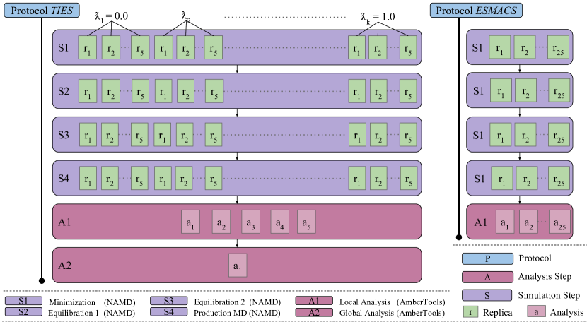
Figure 1: TIES and ESMACS protocols consist of simulations steps followed by analysis step(s). ESMACS contains 25 replicas per simulation step; TIES contains 5 replicas per $\lambda$ window. We model TIES with 13 $\lambda$ windows, spawning 65 replicas in each simulation step. All replicas simulate 6ns.

III-B The Value of Adaptivity

The main driver for adaptivity is that computational campaigns will typically involve compounds with a wide range of chemical properties which can impact the time to convergence and the type of sampling required to gain accurate results. There may be cases where it is important to increase the sampling of phase space, possibly through expanding the ensemble. In general, there is no way to know exactly which calculation setup a particular system requires before runtime.

Another driver of adaptivity is that, on occasion, alchemical methods may converge very slowly. This means that the most effective way to gain accurate and precise free energy results on industrially or clinically relevant timescales is to adapt either the workflow corresponding to a specific protocol or adapt different workflows in relation to each other. The latter is referred to as inter-protocol adaptivity; the former as intra-protocol wherein, for example, the parameter values associated with a specific protocol might change. With thousands of workflows (corresponding to a protocol instances) to adapt in different ways, this has the potential to allow for significant optimization.

In TIES, the change in free energy associated with the transformation is calculated using an adaptive quadrature function which numerically integrates the values of the $\partial U/\partial\lambda$ across the full set of simulated $\lambda$ windows. Obtaining accurate and precise results from TIES using adaptive quadratures requires that the $\lambda$ windows correctly capture the changes of $\partial U/\partial\lambda$ over the transformation. This behavior is highly sensitive to the chemical details of the compounds being studied and varies considerably among candidates. Typically, $\lambda$ windows are evenly spaced between 0 and 1 with the spacing between them set before execution at a distance determined by the simulator to be sufficient for a wide range of systems.

However, the number or the location of the $\lambda$ windows that will most impact the calculation are not known a priori, and varies across candidates. As each window requires multiple simulations, sampling with a high frequency is expensive. Approximations using evenly spaced $\lambda$ windows reach an acceptable accuracy threshold but adaptive placement of $\lambda$ windows is likely to better capture the shape of the $\partial U/\partial\lambda$ curve, leading to more accurate and precise results for a comparable computational cost.

In this work, we focus on intra-protocol adaptivity which relies on intermediate runtime results within a protocol instance to define the following set of simulations. Instead of approximating the placement of all the $\lambda$ windows prior to execution, we run TIES with less $\lambda$ windows and shorter bursts of simulations, analyzing intermediate runtime results (i.e., trajectories) to seed new and ideally placed $\lambda$ windows.

III-C Physical system description

Scientific and computational improvements require validation across a number of protein ligand complexes. We selected 4 proteins and 8 ligands or ligand pairs to run adaptive free energy calculations. The proteins are the Protein tyrosine phosphatase 1B (PTP1B), the Induced myeloid leukemia cell differentiation protein (MC1), tyrosine kinase 2 (TYK2) and the bromodomain-containing protein 4 (BRD4). Four ligands are alchemical transformations from one to another (used in TIES), four are single ligands suitable for absolute free energy calculations (used in ESMACS). All systems were taken from previously published studies [8].

Simulations were set up using our automated tool, BAC [27]. This process includes parametrization of the compounds, solvation of the complexes, electrostatic neutralization of the systems by adding counterions and generation of configurations files for the simulations. The AMBER ff99SB-ILDN [28] force field was used for the proteins, and TIP3P was used for water molecules. Compound parameters were produced using the general AMBER force field (GAFF) [29] with Gaussian 03 [30] to optimize compound geometries and to determine electrostatic potentials at the Hartree–Fock level (with 6-31G** basis functions). The restrained electrostatic potential (RESP) module in the AMBER package [31] was used to calculate the partial atomic charges for the compounds. All systems were solvated in orthorhombic water boxes with a minimum extension from the protein of 14 Å  resulting in systems with approximately 40,000 atoms.

IV High-Throughput Binding Affinity Calculator (HTBAC)

HTBAC is a software system for running ensemble-based free energy protocols adaptively and at scale on HPC resources. Currently, HTBAC supports protocols composed of an arbitrary number of analysis and simulation steps, and relies on the ensemble management system and runtime system provided by the RADICAL-Cybertools (RCT). HTBAC is designed to be extended to support more types of protocols and alternative runtime middleware.

IV-A Requirements

HTBAC satisfies three main requirements: (1) enable the scalable execution of concurrent free energy protocols; (2) abstract protocol specification from execution and resource management; and, (3) enable adaptive execution of protocols.

Computational drug campaigns increasingly depend on scalable ensemble-based protocols. This poses at least two major computational challenges. First, ensemble-based protocols require execution coordination and resource management among ensemble members, within protocols as well as across protocols. Second, the setup of execution environments and data management has to preserve efficient resource utilization. These challenges need to be addressed by HTBAC as well as the underlying ensemble management and runtime system.

Adaptive execution of protocols require the ability to change the control logic of the ensemble execution, based on intermediate results of the ongoing computation. Thus, HTBAC has to support resource redistribution, according to the logic of the adaptive algorithms, enabling the optimization of computational efficiency.

Finally, usability plays an important role in the development of HTBAC. HTBAC has to provide a flexible interface which enables users to easily scale the number of drug candidates and quickly prototype existing and novel free energy protocols.

IV-B Design and Implementation

HTBAC exposes four constructs to specify free energy protocols: Protocol, Simulation, Analysis, and Resource. Protocol enables multiple descriptions of protocol types, while Simulation and Analysis specify simulation and analysis parameters for each protocol. Resource allows to specify the amount of resources needed to execute the given protocols. Together, protocol instances, simulation and analysis parameters, and resource requirements constitute an HTBAC application.

Each protocol models a unique protein ligand physical system. Protocols follow a sequence of simulation and analysis steps, assigning ensemble members to execute independent simulations or analysis. An ensemble member that executes a simulation within a simulation step is referred to as a replica. Each simulation is assigned a different initial velocity, which enables simulations to begin in different parts of the ligand’s phase space.

Individual simulations or analyses with input, output, termination criteria and dedicated resources are designed as a computational task [32]. Aggregates of tasks with dependencies that determine the order of their execution constitute a workflow. In this way, HTBAC encodes $N_{P}$ instances of the P^th protocol as a workflow of computational tasks.

Fig. 2 shows the components and subcomponents of HTBAC. The API enables users to describe protocols in terms of protocol type, simulation and analysis steps, and compute infrastructure requirements. The Descriptor component uses two subcomponents to aggregate protocol descriptions into a single application and resource description. Note that Descriptor can aggregate different types of protocols, with different computing and resource requirements.

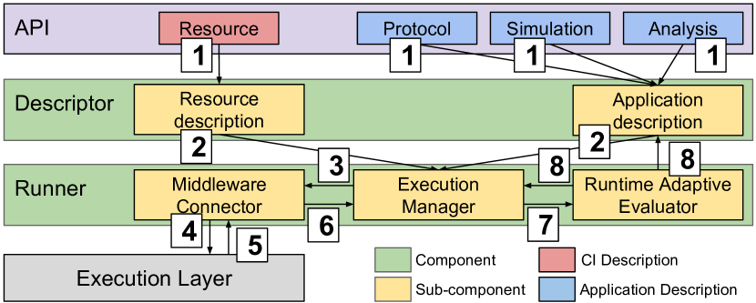
Figure 2: HTBAC architecture. Users specify protocol(s) with multiple simulation and analysis steps. Descriptor derives a single application that Runner executes on an external execution layer. Runtime Adaptive Evaluator enables the execution of adaptive protocols.

The Runner component has three subcomponents: Execution Manager, Middleware Connector and Runtime Adaptive Evaluator. Execution Manager communicates with the execution layer via a connector to coordinate the execution of the application. In principle, HTBAC can use multiple connectors for diverse middleware to access different computing infrastructures.

Middleware Connector converts the application description of HTBAC into a middleware-specific format. Execution Manager can pass the given application to the connector in full or only in parts. This enables to start the execution of an application before its full description is available or to change those parts of the application that still have to be executed. This will enable future capabilities like, for example, to concurrently execute the application on diverse middleware.

Runtime Adaptive Evaluator enables the execution of adaptive applications. This subcomponent can evaluate partial results of an application execution via tailored algorithms. On the base of this evaluation, Runtime Adaptive Evaluator can decide to return the control to Execution Manager or to modify the description of the application that is being executed. In this way, HTBAC implements adaptivity for diverse protocols, allowing users to define arbitrary conditions and algorithms.

HTBAC is implemented in Python as a domain-specific library. All components of HTBAC are implemented as objects that communicate via method calls. HTBAC uses two RCT as building blocks [33]: Ensemble Toolkit (EnTK) and RADICAL-Pilot (RP).

EnTK provides HTBAC capabilities to execute ensemble-based applications [32]. EnTK exposes three constructs: Task, Stage and Pipeline. Tasks contain information regarding an executable, its software environment and its data dependencies. Stages are sets of tasks without mutual dependencies that can execute concurrently. Pipelines are lists of stages, where stages can execute only sequentially. Pipelines can execute independently. HTBAC uses a Middleware Connector for EnTK to encode a protocol instance as a single pipeline that contains stages of individual simulations and analyses tasks.

EnTK is designed to be coupled with different runtime systems. In this paper, EnTK uses RP to execute tasks via pilots. RP supports task-level parallelism and high-throughput by acquiring resources from a computing infrastructure and scheduling tasks on those resources for execution. RP uses RADICAL-SAGA to interface with several resource managers, including SLURM, PBS (pro), and LSF. Pilot systems execute tasks directly on the resources, without queuing them on the infrastructure’s scheduler.

IV-C Execution Model

Users describe one or more protocols alongside their resource requirements via HTBAC’s API. Descriptor takes these descriptions as input and returns an application description (Fig. 2.1). As seen in §IV-B, this application consists of a set or sequence of tasks with a set of resource requirements for their execution.

The application description is passed to the Execution Manager of the Runner component (Fig. 2.2). Execution Manager evaluates the resource requirements, selects a suitable connector (currently only to EnTK), tags each protocol instance of the application with an ID, and passes all or part of the application description to the connector for execution (Fig. 2.3).

The Middleware Connector of the Runner component gets the application description, converting it into a middleware-specific description (EnTK pipelines of stages of tasks) and a resource request. The connector submits this request to the underlying execution layer (Fig. 2.4) and initiates the execution of the application once the execution layer communicates the availability of the resources (Fig. 2.5).

The resource requirements specified via HTBAC’s API include walltime, cores, queue, and user credentials. EnTK derives a resource request from these requirements, converting it into a pilot description for RP. RP converts this pilot requests into a batch script that is submitted to the specified HPC machine. Once the pilot becomes active, EnTK identifies those application tasks that have satisfied dependencies and can be executed concurrently. EnTK’s own Execution Manager uses RP to execute those tasks on pilot’s resources.

HTBAC allows to specify conditions tailored to individual simulation steps of a protocol implementation. We leverage this ability to implement adaptivity by enabling the user to partition protocols into simulation steps and generate new simulation steps at runtime, based on a set of predefined conditions. The user specifies these conditions in an analysis script for the Runtime Adaptive Evaluator subcomponent.

Execution Manager can retrieve the results of simulations (Fig. 2.6) and these results can be evaluated by Runtime Adaptive Evaluator via a user-defined analysis script (Fig. 2.7). Depending on the result of the evaluation, Runtime Adaptive Evaluator may generate new simulation steps, adding them to the application description (Fig. 2.8a) or return the control to Application Manager (Fig. 2.8b) without changing the application. If new simulations are to be generated, the Execution Manager bypasses termination of the application, and passes the added application description to the connector.

In an adaptive scenario, as the number of simulations grows at runtime, the ratio of cores-to-task fluctuates. EnTK’s Execution Manager automatically redistributes an even share of the total requested cores to each simulation. RP allows for new simulations to execute within the pilot’s wall-time, without having to acquire new resources via the resource management system.

IV-D Implementing ESMACS and TIES in HTBAC

In §III-A we define the structure of the ESMACS and TIES protocols. Here we provide skeletons of the TIES protocol implemented in HTBAC. In L. 1 we show a customization of a production MD simulation step.

⬇

1import htbac.protocols.TIES

ties_1 = Protocol(system = ’brd4-1’)

3sim = Simulation(name = ’Production MD’)

... # define simulation conditions

5sim.ensemble(’replica’, range(5))

sim.ensemble(’lambda’, range(13))

7# add simulation configurations to protocol

TIES.step0 = sim

9ties_1.append(TIES.step0)

# assign resources, append protocol to Runner

11runner = Runner(resource = ’ncsa.blue_waters’,

walltime = 60)

13runner.add_protocol(protocol = ties_1)

# launch application

15runner.run()

Listing 1: TIES protocol implemented with HTBAC. We import the predefined protocol ‘TIES’. We assign the physical system to the protocol, we instantiate a simulation, customize its steps (replica, lambda) and assign it to the TIES’s step0. We instantiate Runner with a resource request and pass the protocol to it.

In §IV-C we show HTBAC’s adaptive execution capabilities. In L. 2 we provide an intra-protocol adaptive implementation of TIES, based on the use-case of §III-B.

⬇

1# we start with the same previous implementation

# provide runner with two flags

3runner.run(save_output = True, terminate = False)

# specify adaptivity script

5requested_lambdas = AdaptiveQuadrature()

sim1 = Simulation(name = ’production MD 2’)

7 ...

sim1.ensemble(’replica’, range(5))

9sim1.ensemble(’additional lambdas’,

requested_lambdas)

11TIES.step1 = sim1

ties_1.append(TIES.step1)

13runner.add_protocol(protocol = ties_1)

runner.run(terminate = True)

Listing 2: Adaptive TIES protocol implemented with HTBAC. Assuming L. 1, we run Runner retrieving runtime results, we specify an adaptivity script for the evaluator, create TIES’s step1. The analysis script operates on partial simulation results, generating new simulation conditions for the next simulation step.

V Experiments

Typically, a computational campaign for drug discovery explores a large number of drug candidates by running several workflows multiple times, each requiring thousands of concurrent simulations. Before embarking on a campaign that will utilize 150 million core-hours on NCSA Blue Waters, we perform experiments to characterize the weak and strong scaling performance of HTBAC and its overheads on Blue Waters. We validate the results of the free energy calculations produced using HTBAC against published results.

Given that protocols like TIES are more computationally demanding than protocols like ESMACS, it is paramount to use resources efficiently, especially for campaigns that have a predefined computational budget. As described in § III and IV, adaptive simulation methods have the potential to reduce the number of simulations without a loss in accuracy and with a lower computational load. We run experiments with an adaptive implementation of TIES in HTBAC, measuring the benefits in terms of accuracy, reduced number of simulations and computational load.

V-A Experiment Setup

Table I shows 9 experiments we designed to characterize the behavior of HTBAC on Blue Waters. Each experiment executes the ESMACS and/or TIES protocol for different physical systems. Experiments 1–6 use the BRD4 physical system provided by GlaxoSmithKline, while experiments 7–9 utilize the PTP1B, MC1, and TYK2 physical systems.

TABLE I: Parameters of scalability and adaptivity experiments.

ID	Type of Experiment	Physical System(s)	Protocol(s)	No. Protocol(s)	Total Cores
1	Weak scaling	BRD4	ESMACS	(2, 4, 8, 16)	1600, 3200, 6400
2	Weak scaling	BRD4	TIES	(2, 4, 8)	4160, 8320, 16640
3	Weak scaling	BRD4	ESMACS + TIES	(2, 4, 8)	5280, 10560, 21120
4	Strong scaling	BRD4	TIES	(8, 8, 8)	16640, 8320, 4160
5	Strong scaling	BRD4	ESMACS	(16, 16, 16)	6400, 3200, 1600
6	Strong scaling	BRD4	ESMACS + TIES	(20, 20, 20)	22120, 10560, 5280
7	Non-adaptivity	PTP1B, MC1, TYK2	TIES	(1, 1, 1)	2080, 2080, 2080
8	Adaptivity	PTP1B, MC1, TYK2	TIES	(1, 1, 1)	2080, 2080, 2080
9	Reference	PTP1B, MC1, TYK2	TIES	(1, 1, 1)	10400, 10400, 10400

Experiment 1 and 2 measure the weak scaling of HTBAC using the ESMACS and TIES protocols. Experiments 3 uses both the TIES and ESMACS protocols, characterizing the weak scaling of heterogeneous protocol executions. Experiments 4 and 5 measure the strong scaling of HTBAC using a fix number of instances of the ESMACS and TIES protocols. Experiments 6 uses both the TIES and ESMACS protocols, characterizing the strong scaling of heterogeneous protocol executions. Experiments 7–9 characterize nonadaptive and adaptive simulation methods using the TIES protocol.

In each weak scaling experiment (1–3), we keep the ratio between resources allocated and protocol instances constant. Consistently, for each experiment we progressively increase both the number of cores (i.e., measure of resource) and the number of protocol instances by a factor of 2. In each strong scaling experiment (4–6), we change the ratio between resources allocated and the number of protocol instances: we fix the number of protocol instances and reduce the number of cores by a factor of 2.

Weak scaling experiments provide insight into the size of the workload that can be executed in a given amount of time, while strong scaling experiments show how the time duration of the workload scales when adding resources. For all the weak and strong scaling experiments we characterize the overheads of HTBAC, EnTK and RP, and we show an approximation of the time taken by the resources to become available. This offers insight about the impact of HTBAC and its runtime system on the time to completion of each workload. In [34], we show baseline performance of HTBAC using ESMACS with a null workload.

For weak and strong scaling experiments, we reduced the number of time-steps of the protocols and omitted the analysis steps $S5$ and $S6$ of their workflows (Fig. 1). These simplifications are consistent with characterizing scalability performance instead of simulation duration. The time-steps are set to enable the physical systems to reach steady-state. For the experiments 1–6 we used the following time-steps: $S1=1000$; $S2=5000$; $S3=5000$; and $S4=50000$.

We measure the following durations for Experiments 1–6:

• Total Task Execution Time: Time taken by all the task executables to run on the computing infrastructure.

• HTBAC Overhead: Time taken to instantiate HTBAC, and validate and process the application description.

• EnTK and RP Overhead: Time taken by EnTK and RP to manage the execution of tasks.

• aprun Overhead: Time taken by aprun to launch tasks on Blue Waters.

Note that once RP relinquishes the control flow to aprun, the precise time at which aprun schedules each task on a compute node and the MD kernel of each task begins execution cannot be measured. Instead, for each task, we measure the difference between the task execution time and its NAMD kernel execution time, provided by the NAMD output logs. In this way, we approximate the time taken by aprun to launch the task. Once aggregated, these measures constitute what we defined as aprun Overhead. The summation of all durations provides the average wall-time of the pilot job.

Experiments 7–9 compare the accuracy and time to solution of nonadaptive and adaptive simulation methods. For the nonadaptive simulation method of Experiment 7 we use 13 preassigned and approximated $\lambda$ windows, consistent with the value reported in Ref. [8]. In this way, we produce 65 concurrent simulations for stages $S1$–$S4$ of TIES (see Fig. 1). The production simulation stage $S4$ executes each simulation for $4\text{\,}\mathrm{ns}$. Stage $S5$ has 5 analysis tasks which aggregate the simulation results of $S4$. The global analysis stage $S6$ has a single task that aggregates the results from $S5$.

In the adaptive implementation 3, we initialize the TIES protocol with 3 $\lambda$ windows, obtaining 15 replicas. We separate stage $S4$ of each TIES replica into 4 sub-stages. Each sub-stage runs a $1\text{\,}\mathrm{ns}$ simulation, followed by an adaptive quadratures analysis which estimates free energy errors with respect to each interval of two $\lambda$ values.

We use Experiment 9 to compare the adaptive and non-adaptive execution of TIES. We use 65 simulations, derived from 13 equally spaced $\lambda$ windows to calculate the free energy with high accuracy. This creates a baseline against which to compare the adaptive and non-adaptive results.

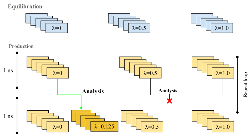
Figure 3: Adaptive workflow for TIES. After equilibrating 3 $\lambda$, the first stage starts. This is followed by analysis at every $\lambda$ interval, to decide whether to add a new window in between. In our implementation, the simulation-analysis cycle is repeated for 4 simulation steps, not shown here.

We assigned the following simulation time-steps in Experiment 7 and 9: $S1=3000$; $S2=50000$; $S3=50000$; and $S4=2000000$. The adaptive simulation of Experiment 8 uses the same time-steps, apart from $S4$ which is divided into 4 sub-stages of 500000 time-steps each.

We performed all the experiments on Blue Waters, a 26868 node Cray XE6/XK6 SuperComputer with peak performance of 13.3 petaFLOPS managed by NCSA. Consistent with NCSA policies, we initiated the experiments from a virtual machine outside NCSA, avoiding to run persistent process on the NCSA login node. We used HTBAC 0.1, EnTK 0.6, and RP 0.47 and the NAMD-MPI MD kernel, and launched via the aprun command. For the analysis stages in the TIES protocol we used AmberTools.

NCSA sets a system policy on the maximum number of processes that aprun can spawn, limiting the number of concurrent tasks we can execute on Blue Waters to $\approx$450. During the execution of Experiment 2, we observed failing tasks with 8 TIES protocol instances, i.e., 520 concurrent tasks. In a trial of 10 repetitions at this scale, we observed an average of $70\pm 6.67$ failing tasks. More data would be required to model the distribution type of these results.

NCSA allows to run only one MPI application for each compute node. Thus, we run each MD simulation with 32 cores (i.e., one compute node) even if our performance of NAMD on Blue Waters indicated that 16 cores offers the best trade-off between computing time and communication overhead.

V-B Weak Scaling Characterization

Fig. 4(a) shows the weak scaling of HTBAC with the TIES protocol. Each instance of the TIES protocol contains a single pipeline with 4 stages and 65 concurrent tasks. We increase the number of protocol instances linearly, between 2 and 8. When scaling to 8 protocol instances, we execute more than 450 concurrent tasks, the average limit supported by aprun, as described in §V-A. This introduces some failures that contribute to a slight degradation in performance.

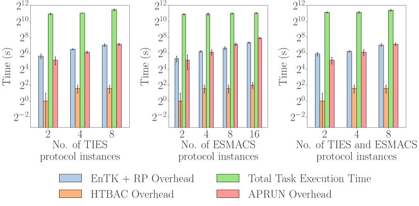
Figure 4: Weak scaling of HTBAC. The ratio number of protocol instances to resources is constant. Task Execution Time, and HTBAC, EnTK+RP, aprun overheads with (a) TIES (Experiment 1), (b) ESMACS (Experiment 2), and (c) TIES and ESMACS (Experiment 3).

Fig. 4(b) shows the weak scaling of HTBAC with the ESMACS protocol. We increase the number of instances linearly, between 2 and 16. Each ESMACS protocol contains 1 pipeline with 4 stages and 25 concurrent tasks.

Fig. 4(c) shows the weak scaling of HTBAC with instances of both TIES and ESMACS protocols. Also in this case, we scale the instances of both protocols linearly, between 2 and 8. The first configuration shows 1 ESMACS and 1 TIES protocol, and with each increase in scale we double the number of protocols. Experiments 2 and 3 show scaling ranges within the limit of the maximum number of concurrent tasks we can successfully execute on Blue Waters.

For all weak scaling experiments (1–3) we use physical systems from the BRD4-GSK library with the same number of atoms and similar chemical properties. The uniformity of these physical systems ensures a consistent workload with insignificant variability when characterizing their performance under different conditions.

In all weak scaling experiments (Fig. 4) we observe that the value of Total Task Execution Time (green bar) shows minimal variation as the number of protocol instances increases, suggesting that HTBAC is invariant to the protocol. We conclude that HTBAC shows near-ideal weak scaling behavior under these conditions.

The HTBAC overhead depends mostly on the number of protocol instances that need to be generated for an application. This overhead shows a super linear increase as we grow the number of protocol instances, but the duration of the overhead is negligible when compared to Total Task Execution Time.

The aprun overhead increases as we approach the limit of concurrent aprun processes that can be executed on Blue Waters. For example, when scaling to 8 TIES protocol instances (Fig. 4(a)), we see that the increase in aprun overhead occurs due to task failure. This is explained by noticing that attempts to relaunch failed tasks require additional communication among the nodes that were running the tasks and the MOM Nodes from which the execution is coordinated.

EnTK and RP overheads mostly depend on the number of tasks that need to be translated in-memory from a Python object to a task description [34, 35]. As such, those overheads are expected to grow proportionally to the number of tasks, as observed in Fig. 4, blue bars.

The RP overhead is calculated by measuring and aggregating the execution time of the RP components that manage and coordinate the execution of the protocol instances. Among these components, the task scheduler of RP introduces the largest overhead. Due to the general scheduling algorithm loaded by default in RP, the task scheduling overhead scales linearly with the number of tasks that need to be scheduled.

In comparison to Total Task Execution Time, the EnTK and RP overheads are an order of magnitude shorter, yet they directly contribute to the total duration of the application execution. Based on Fig. 4, we approximate the use of our systems will results in $\approx 15\%$ additional usage of resource allocation. This overhead can be substantially reduced by using a special-purpose scheduler for RP as illustrated in Ref. [35].

V-C Strong Scaling Characterization

In Experiment 4 we fix the number of instances of the TIES protocol to 8 (due to the described aprun limitations) and we vary the amount of resources between 4160, 8320 and 16640 cores. Assuming the definition of ‘generation’ in §V-A, given 4160 cores, we can execute 4 generations of 130 concurrent tasks; with 8320 cores, 2 generations of 260 tasks; and with 16640 cores, 1 generation of 520 tasks.

In Experiment 5 we fix the number of instances of the ESMACS protocols to 16 and vary the amount of resources between 3200, 6400 and 12800 cores. In this way, we obtain the same number of generations as in Experiment 4.

In Experiment 6 we fix the number of instances of the ESMACS and TIES protocols to 16 and 4 respectively, and vary the amount of resources between 5280, 10560 and 22120 cores. In this way, we obtain the same number of generations as in Experiment 4 and 5.

Fig. 5 shows a linear speedup in Total Task Execution Time for both experiments, proportional to the increase in the number of cores. The availability of more resources for a fixed number of protocols explains this behavior. Overheads remain essentially constant for both experiments when increasing the number of cores. The scheduling of the number of tasks, as opposed to the amount of resources, is the main driver of EnTK and RP overheads (Ref. [35]).

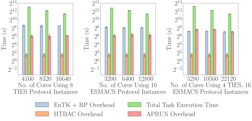
Figure 5: Strong scaling of HTBAC. The number of protocol instances is fixed while the number of cores increases. Task Execution Time, and HTBAC, EnTK+RP, aprun overheads with (a) TIES (Experiment 4), ESMACS (Experiment 5) and ESMACS + TIES (Experiment 6).

V-D Validation

In order to validate the correctness of the results produced in Experiment 1–6, using HTBAC and the BRD4-GSK physical systems, we compare our results with those previously published in Wan et al. [11]. In this way, we can confirm that we calculated the correct binding free energies values.

We validated our implementation selecting a subset of the protein ligand systems used in Wan et al. [11]: ligand transformations 3 to 1, 4, and 7. We then performed a full simulation on all 3 systems and calculated the binding affinity using HTBAC.

The results of our experiments, collected in Table II, show that all three $\Delta\Delta$G values are within error bars of the original study, validating the results we produced with HTBAC.

TABLE II: Validation of HTBAC results against published and experimental values

System	HTBAC ($\mathrm{kcal}\text{\,}{\mathrm{mol}}^{-1}$)	Wan et al. ($\mathrm{kcal}\text{\,}{\mathrm{mol}}^{-1}$)	Experiment ($\mathrm{kcal}\text{\,}{\mathrm{mol}}^{-1}$)
BRD4 3 to 1	$0.39(10)$	$0.41(4)$	$0.30(9)$
BRD4 3 to 4	$0.02(12)$	$0.01(6)$	$0.00(13)$
BRD4 3 to 7	$-0.88(17)$	$-0.90(8)$	$-1.30(11)$

V-E Adaptive Experiments

The design of HTBAC permits enhancing protocols while continuing to use “static” simulation engines. To this end, we implemented two adaptive methods using HTBAC: adaptive quadrature and adaptive termination. Both of these methods use the features of adaptivity offered in HTBAC to scale to large number of concurrent simulations and to increase convergence rate and obtain more accurate scientific results.

The aim of introducing adaptive quadrature for alchemical free energy calculation protocols (e.g., TIES) is to reduce time to completion while maintaining (or increasing) the accuracy of the results. Time to completion is measured by the number of core-hours consumed by the simulations. Accuracy is defined as the error with respect to a reference value, calculated via a dense $\lambda$ window spacing (65 windows). This reference value is used to establish the accuracy of the non-adaptive protocol (which has 13 $\lambda$ windows) and the adaptive protocol (which has a variable number of $\lambda$ windows, determined at run time).

One of the input parameters of the adaptive quadrature algorithm is the desired acceptable error threshold of the estimated integral. We set this threshold to the error of the non-adaptive algorithm calculated via the reference value. The algorithm then tries to minimize the number of $\lambda$ windows constrained by the accuracy requirement.

Figure 6: Quantifying the benefits of the adaptive quadrature simulations. (top) The error of the adaptive run is reduced for all 5 test systems, sometimes by a significant amount. It has been shown that reproducibility of free energy calculations can be achieved up to $0.2\text{\,}\mathrm{kcal}\text{\,}{\mathrm{mol}}^{-1}$ [36]. The adaptive algorithm brings down the error of the nonadaptive simulations below this threshold, ensuring that results are also reproducible. (bottom) Resource consumption is reduced, except for one of the systems, where the low error threshold required more $\lambda$ windows.

Table III shows the results of running adaptive quadrature on 5 protein ligand systems, comparing the Total Task Execution Time and accuracy versus the non-adaptive case. The number of lambda windows are reduced on average by $32\text{\,}\mathrm{\char 37\relax}$, hence reducing Total Task Execution Time by the same amount. The error on the adaptive results is also decreased, on average by $77\text{\,}\mathrm{\char 37\relax}$ (see fig. 6). More importantly, the error on all of the systems are reduced to below $0.2\text{\,}\mathrm{kcal}\text{\,}{\mathrm{mol}}^{-1}$, which has recently been shown to be the upper bound of reproducibility across different simulation engines [36].

The Total Task Execution Time of the TYK2 L7–L8 system has increased for the adaptive run by 1 $\lambda$ window, compared to the non-adaptive case. This is due to the non-adaptive error being very low, and matching that same accuracy required the use of a large number of windows. Nonetheless due to the efficient placing of the windows, the accuracy of the free energy still increased by $40\text{\,}\mathrm{\char 37\relax}$.

TABLE III: Comparing results of adaptive, non-adaptive and reference runs.

System	Ref $\Delta\Delta$G ($\mathrm{kcal}\text{\,}{\mathrm{mol}}^{-1}$)	Non-adaptive $\Delta\Delta$G ($\mathrm{kcal}\text{\,}{\mathrm{mol}}^{-1}$)	Adaptive $\Delta\Delta$G ($\mathrm{kcal}\text{\,}{\mathrm{mol}}^{-1}$)	No. of $\lambda$ windows	Decrease in TTX	Increase in accuracy
PTP1B L1-L2	$-58.51$	$-57.87(64)$	$-58.60(9)$	$10$	$23$$\mathrm{\char 37\relax}$	$86$$\mathrm{\char 37\relax}$
PTP1B L10-L12	$1.83$	$2.05(22)$	$1.94(7)$	$6$	$54$$\mathrm{\char 37\relax}$	$68$$\mathrm{\char 37\relax}$
MCL1 L32-L38	$2.13$	$2.33(20)$	$2.14(1)$	$7$	$46$$\mathrm{\char 37\relax}$	$95$$\mathrm{\char 37\relax}$
TYK2 L4-L9	$-28.69$	$-28.25(44)$	$-28.67(1)$	$7$	$46$$\mathrm{\char 37\relax}$	$98$$\mathrm{\char 37\relax}$
TYK2 L7-L8	$4.97$	$4.92(5)$	$5.00(3)$	$14$	$-8$$\mathrm{\char 37\relax}$	$40$$\mathrm{\char 37\relax}$

Fig. 7 compares the error on the adaptive and non-adaptive simulations as a time series plot. As fewer lambda windows are calculated the adaptive algorithm uses less resources. Remarkably, the error is drastically reduced as the windows are placed adaptively to capture the changes in function.

Figure 7: Plot of the error estimate as a function of the resource consumption, comparing the adaptive and nonadaptive simulations. The error estimate converges for both simulations but the window placement of the adaptive simulation considerably lowered the error.

Adaptive quadrature is specific to alchemical free energy calculations. Adaptive termination, the second adaptive method implemented in HTBAC, offers dynamic termination for any simulation protocol that has as its aim the prediction of an observable value. The protocol monitors the convergence of the observable as the simulation progresses, and stops the execution when a criterion has been met. Non-adaptive protocols usually have a predefined simulation time, set based on the assumption that the simulation will converge by that time. This means that in practical examples the simulation might have converged before the predefined simulation time.

In the original TIES protocol the production part of the simulation has to be run for $4\text{\,}\mathrm{ns}$ and the results are analyzed thereafter. This assumes that all systems need this simulation time for the results to converge. In reality, certain systems could converge faster, therefore one can terminate the simulation before the static $4\text{\,}\mathrm{ns}$ end. This would lead to faster time to insight and less compute resources consumed. Adaptive termination was implemented in HTBAC by having a checkpoint every $\tau=$0.5\text{\,}\mathrm{ns}$$ in the simulation. Fig. 8 shows how the observable for a specific simulation changes as a function of resource consumption. At every checkpoint the convergence is evaluated, and the simulation is indeed terminated earlier than the non-adaptive protocol would suggest. Table IV shows results that the adaptively terminated TIES protocol saves compute resources and reduces time to insight on average by $16\text{\,}\mathrm{\char 37\relax}$ for the physical systems tested.

Figure 8: Plot of the free energy as a function of the resources consumed (hence simulation time). The adaptive termination algorithm checks the convergence of the observable every $\tau=$0.5\text{\,}\mathrm{ns}$$ and if the threshold ($0.01\text{\,}\mathrm{kcal}\text{\,}{\mathrm{mol}}^{-1}$) has been met, terminates the simulation.

TABLE IV: Simulation time of non-adaptive and adaptively terminated runs for a given convergence criterion

System	Non-adaptive	Adaptive	Decrease in TTX
PTP1B L10-L12	$6.0$$\mathrm{ns}$	$5.0$$\mathrm{ns}$	$16.7$$\mathrm{\char 37\relax}$
TYK2 L4-L9	$6.0$$\mathrm{ns}$	$5.5$$\mathrm{ns}$	$8.3$$\mathrm{\char 37\relax}$
TYK2 L7-L8	$6.0$$\mathrm{ns}$	$4.5$$\mathrm{ns}$	$25.0$$\mathrm{\char 37\relax}$

VI Discussion and Conclusion

Ensemble-based binding affinity protocols have considerable predictive potential in computational drug campaigns. As drug screening can cover millions of compounds and hundreds of millions of core-hours, it is important for binding affinity calculations to optimize the accuracy and precision of results. However, the optimal protocol configuration for a given compound is difficult to determine a priori, thus requiring runtime adaptations to workflow executions. We introduce HTBAC to enable scalable and adaptive binding affinity energy calculations on HPC.

Specifically, this paper makes the following contributions: (1) shows how adaptive execution of ensemble-based free energy protocol (TIES) improve binding affinity accuracy given a fixed amount of computing resources; (2) characterizes HTBAC, the software system we developed to enable the adaptive execution of ensemble-based binding affinity protocols on HPC; and (3) shows the capability to execute adaptive applications at scale, validating their scientific results.

We characterize the performance of HTBAC on NCSA Blue Waters. We show near-ideal weak and strong scaling behavior for ESMACS and TIES, individually and together, reaching scales of 21,120 cores. Furthermore, we validate binding free energies computed using HTBAC with both experimental and previously published computational results.

We compare resource consumption and free energy accuracy in our adaptive and non-adaptive TIES results. Using the adaptive quadrature algorithm, we show improvements in $\Delta\Delta$G on average by 77% over the 5 physical systems tested. By reducing the $\lambda$ windows on average by 32%, we reduce execution time by the same amount. The adaptive termination implementation of the TIES protocol saves compute resources and reduces time to solution on average by 16%. To the best of our knowledge, adaptive TIES protocols have not been benchmarked against non-adaptive implementations before.

Software and Data

All experimental data can be found at https://github.com/radical-experiments/htbac-escience-18. HTBAC (MIT license) can be found at: https://github.com/radical-cybertools/htbac

References

- [1] S. M. Paul, D. S. Mytelka, C. T. Dunwiddie, C. C. Persinger, B. H. Munos, S. R. Lindborg, and A. L. Schacht, “How to improve R&D productivity: the pharmaceutical industry’s grand challenge,” Nature Reviews Drug Discovery, vol. 9, no. 3, pp. 203–214, Mar. 2010. [Online]. Available: https://www.nature.com/articles/nrd3078
- [2] D. L. Mobley and P. V. Klimovich, “Perspective: Alchemical free energy calculations for drug discovery,” The Journal of Chemical Physics, vol. 137, no. 23, p. 230901, 2012. [Online]. Available: https://doi.org/10.1063/1.4769292
- [3] A. S. J. S. Mey, J. J. Jiménez, and J. Michel, “Impact of domain knowledge on blinded predictions of binding energies by alchemical free energy calculations,” Journal of Computer-Aided Molecular Design, Nov 2017. [Online]. Available: https://doi.org/10.1007/s10822-017-0083-9
- [4] J. Yin, N. M. Henriksen, D. R. Slochower, M. R. Shirts, M. W. Chiu, D. L. Mobley, and M. K. Gilson, “Overview of the sampl5 host–guest challenge: Are we doing better?” Journal of Computer-Aided Molecular Design, vol. 31, no. 1, pp. 1–19, Jan 2017. [Online]. Available: https://doi.org/10.1007/s10822-016-9974-4
- [5] L. Wang, Y. Wu, Y. Deng, B. Kim, L. Pierce, G. Krilov, D. Lupyan, S. Robinson, M. K. Dahlgren, J. Greenwood, D. L. Romero, C. Masse, J. L. Knight, T. Steinbrecher, T. Beuming, W. Damm, E. Harder, W. Sherman, M. Brewer, R. Wester, M. Murcko, L. Frye, R. Farid, T. Lin, D. L. Mobley, W. L. Jorgensen, B. J. Berne, R. A. Friesner, and R. Abel, “Accurate and Reliable Prediction of Relative Ligand Binding Potency in Prospective Drug Discovery by Way of a Modern Free-Energy Calculation Protocol and Force Field,” J. Am. Chem. Soc., vol. 137, no. 7, pp. 2695–2703, Feb. 2015. [Online]. Available: http://pubs.acs.org/doi/abs/10.1021/ja512751q
- [6] A. Ganesan, M. L. Coote, and K. Barakat, “Molecular dynamics-driven drug discovery: leaping forward with confidence,” Drug Discovery Today, vol. 22, no. 2, pp. 249 – 269, 2017. [Online]. Available: http://www.sciencedirect.com/science/article/pii/S1359644616304147
- [7] A. Weis, K. Katebzadeh, P. Söderhjelm, I. Nilsson, and U. Ryde, “Ligand affinities predicted with the mm/pbsa method: dependence on the simulation method and the force field,” Journal of medicinal chemistry, vol. 49, no. 22, pp. 6596–6606, 2006.
- [8] A. P. Bhati, S. Wan, D. W. Wright, and P. V. Coveney, “Rapid, accurate, precise and reliable relative free energy prediction using ensemble based thermodynamic integration,” J. Chem. Theory Comput., vol. 13, no. 1, pp. 210–222, 2017.
- [9] J. C. Phillips, R. Braun, W. Wang, J. Gumbart, E. Tajkhorshid, E. Villa, C. Chipot, R. D. Skeel, L. Kalé, and K. Schulten, “Scalable molecular dynamics with NAMD.” J. Comput. Chem., vol. 26, no. 16, pp. 1781–1802, 2005. [Online]. Available: http://dx.doi.org/10.1002/jcc.20289
- [10] T. P. Straatsma and J. A. McCammon, “Multiconfiguration thermodynamic integration,” The Journal of Chemical Physics, vol. 95, no. 2, pp. 1175–1188, Jul. 1991. [Online]. Available: http://aip.scitation.org/doi/10.1063/1.461148
- [11] S. Wan, A. P. Bhati, S. J. Zasada, I. Wall, D. Green, P. Bamborough, and P. V. Coveney, “Rapid and reliable binding affinity prediction of bromodomain inhibitors: a computational study,” J. Chem. Theory Comput., vol. 13, no. 2, pp. 784–795, 2017.
- [12] P. V. Klimovich, M. R. Shirts, and D. L. Mobley, “Guidelines for the analysis of free energy calculations,” Journal of Computer-Aided Molecular Design, vol. 29, no. 5, pp. 397–411, May 2015. [Online]. Available: http://link.springer.com/10.1007/s10822-015-9840-9
- [13] L. N. Naden and M. R. Shirts, “Rapid Computation of Thermodynamic Properties over Multidimensional Nonbonded Parameter Spaces Using Adaptive Multistate Reweighting,” Journal of Chemical Theory and Computation, vol. 12, no. 4, pp. 1806–1823, Apr. 2016. [Online]. Available: http://pubs.acs.org/doi/10.1021/acs.jctc.5b00869
- [14] J. W. Kaus, L. T. Pierce, R. C. Walker, and J. A. McCammon, “Improving the Efficiency of Free Energy Calculations in the Amber Molecular Dynamics Package,” Journal of Chemical Theory and Computation, vol. 9, no. 9, pp. 4131–4139, Sep. 2013. [Online]. Available: http://pubs.acs.org/doi/10.1021/ct400340s
- [15] P. Kasson and S. Jha, “Adaptive ensemble simulations of biomolecules,” Current Opinions in Structural Biology, 2018, https://arxiv.org/pdf/1809.04804.pdf.
- [16] V. Balasubramanian, T. Jensen, M. Turilli, P. Kasson, M. Shirts, and S. Jha, “Implementing adaptive ensemble biomolecular applications at scale,” 2018, https://arxiv.org/pdf/1804.04736.pdf.
- [17] M. Karplus and J. Kuriyan, “Molecular dynamics and protein function.” Proc. Natl. Acad. Sci. U.S.A., vol. 102, pp. 6679–6685, May 2005.
- [18] G. R. Bowman, D. L. Ensign, and V. S. Pande, “Enhanced modeling via network theory: Adaptive sampling of markov state models,” Journal of Chemical Theory and Computation, vol. 6, no. 3, pp. 787–794, 2010. [Online]. Available: https://doi.org/10.1021/ct900620b
- [19] D. J. Earl and M. W. Deem, “Parallel tempering: Theory, applications, and new perspectives,” Phys. Chem. Chem. Phys., vol. 7, pp. 3910–3916, 2005. [Online]. Available: http://dx.doi.org/10.1039/B509983H
- [20] J. Hritz and C. Oostenbrink, “Hamiltonian replica exchange molecular dynamics using soft-core interactions,” Journal of Chemical Physics, vol. 128, no. 14, p. 144121, 2008. [Online]. Available: http://dx.doi.org/10.1063/1.2888998
- [21] J. Kim, J. E. Straub, and T. Keyes, “Replica exchange statistical temperature molecular dynamics algorithm,” The Journal of Physical Chemistry B, vol. 116, no. 29, pp. 8646–8653, 2012, pMID: 22540354. [Online]. Available: https://doi.org/10.1021/jp300366j
- [22] A. P. Lyubartsev, A. A. Martsinovski, S. V. Shevkunov, and P. N. Vorontsov-Velyaminov, “New approach to Monte Carlo calculation of the free energy: Method of expanded ensembles,” The Journal of Chemical Physics, vol. 96, no. 3, pp. 1776–1783, Feb. 1992. [Online]. Available: http://aip.scitation.org/doi/10.1063/1.462133
- [23] A. de Ruiter, S. Boresch, and C. Oostenbrink, “Comparison of thermodynamic integration and bennett acceptance ratio for calculating relative protein-ligand binding free energies,” Journal of Computational Chemistry, vol. 34, no. 12, pp. 1024–1034, 2013. [Online]. Available: https://onlinelibrary.wiley.com/doi/abs/10.1002/jcc.23229
- [24] A. de Ruiter and C. Oostenbrink, “Extended thermodynamic integration: Efficient prediction of lambda derivatives at nonsimulated points,” Journal of Chemical Theory and Computation, vol. 12, no. 9, pp. 4476–4486, 2016, pMID: 27494138. [Online]. Available: http://dx.doi.org/10.1021/acs.jctc.6b00458
- [25] I. Massova and P. Kollman, “Computational alanine scanning to probe protein-protein interactions: A novel approach to evaluate binding free energies,” J. Am. Chem. Soc., vol. 121, no. 36, pp. 8133–8143, 1999.
- [26] T. P. Straatsma and H. J. C. Berendsen, “Free energy of ionic hydration: Analysis of a thermodynamic integration technique to evaluate free energy differences by molecular dynamics simulations,” The Journal of Chemical Physics, vol. 89, no. 9, pp. 5876–5886, 1988. [Online]. Available: https://doi.org/10.1063/1.455539
- [27] S. K. Sadiq, D. W. Wright, S. J. Watson, S. J. Zasada, I. Stoica, and P. Coveney, “Automated Molecular Simulation Based Binding Affinity Calculator for Ligand-Bound HIV-1 Proteases,” J. Chem. Inf. Model., vol. 48, no. 9, pp. 1909–1919, 2008.
- [28] K. Lindorff-Larsen, S. Piana, K. Palmo, P. Maragakis, J. L. Klepeis, R. O. Dror, and D. E. Shaw, “Improved side-chain torsion potentials for the Amber ff99SB protein force field,” Proteins: Structure, Function, and Bioinformatics, vol. 78, no. 8, pp. 1950–1958, 2010. [Online]. Available: http://dx.doi.org/10.1002/prot.22711
- [29] J. Wang, R. M. Wolf, J. W. Caldwell, P. A. Kollman, and D. A. Case, “Development and testing of a general Amber force field.” J. Comput. Chem., vol. 25, no. 9, pp. 1157–1174, 2004. [Online]. Available: http://dx.doi.org/10.1002/jcc.20035
- [30] M. J. Frisch, G. W. Trucks, H. B. Schlegel, G. E. Scuseria, M. A. Robb, J. R. Cheeseman, J. A. Montgomery, Jr., T. Vreven, K. N. Kudin, J. C. Burant, J. M. Millam, S. S. Iyengar, J. Tomasi, V. Barone, B. Mennucci, M. Cossi, G. Scalmani, N. Rega, G. A. Petersson, H. Nakatsuji, M. Hada, M. Ehara, K. Toyota, R. Fukuda, J. Hasegawa, M. Ishida, T. Nakajima, Y. Honda, O. Kitao, H. Nakai, M. Klene, X. Li, J. E. Knox, H. P. Hratchian, J. B. Cross, V. Bakken, C. Adamo, J. Jaramillo, R. Gomperts, R. E. Stratmann, O. Yazyev, A. J. Austin, R. Cammi, C. Pomelli, J. W. Ochterski, P. Y. Ayala, K. Morokuma, G. A. Voth, P. Salvador, J. J. Dannenberg, V. G. Zakrzewski, S. Dapprich, A. D. Daniels, M. C. Strain, O. Farkas, D. K. Malick, A. D. Rabuck, K. Raghavachari, J. B. Foresman, J. V. Ortiz, Q. Cui, A. G. Baboul, S. Clifford, J. Cioslowski, B. B. Stefanov, G. Liu, A. Liashenko, P. Piskorz, I. Komaromi, R. L. Martin, D. J. Fox, T. Keith, M. A. Al-Laham, C. Y. Peng, A. Nanayakkara, M. Challacombe, P. M. W. Gill, B. Johnson, W. Chen, M. W. Wong, C. Gonzalez, and J. A. Pople, “Gaussian 03, Revision C.02,” Gaussian, Inc., Wallingford, CT, 2004.
- [31] D. A. Case, T. E. Cheatham, T. Darden, H. Gohlke, R. Luo, K. M. Merz, A. Onufriev, C. Simmerling, B. Wang, and R. J. Woods, “The Amber biomolecular simulation programs.” J. Comput. Chem., vol. 26, no. 16, pp. 1668–1688, 2005. [Online]. Available: http://dx.doi.org/10.1002/jcc.20290
- [32] V. Balasubramanian, M. Turilli, W. Hu, M. Lefebvre, W. Lei, R. T. Modrak, G. Cervone, J. Tromp, and S. Jha, “Harnessing the power of many: Extensible toolkit for scalable ensemble applications,” in 2018 IEEE International Parallel and Distributed Processing Symposium, IPDPS 2018, Vancouver, BC, Canada, May 21-25, 2018, 2018, pp. 536–545. [Online]. Available: https://doi.org/10.1109/IPDPS.2018.00063
- [33] M. Turilli, A. Merzky, V. Balasubramanian, and S. Jha, “Building blocks for workflow system middleware,” in 18th IEEE/ACM International Symposium on Cluster, Cloud and Grid Computing, CCGRID 2018, Washington, DC, USA, May 1-4, 2018, 2018, pp. 348–349. [Online]. Available: https://doi.org/10.1109/CCGRID.2018.00051
- [34] J. Dakka and et al, “High-throughput binding affinity calculations at extreme scales,” accepted Computational Approaches for Cancer Workshop, SC’17, 2017, http://arxiv.org/abs/1712.09168.
- [35] A. Merzky, M. Turilli, M. Maldonado, and S. Jha, “Design and performance characterization of radical-pilot on titan,” CoRR, vol. abs/1801.01843, 2018. [Online]. Available: http://arxiv.org/abs/1801.01843
- [36] H. H. Loeffler, S. Bosisio, G. Duarte Ramos Matos, D. Suh, B. Roux, D. L. Mobley, and J. Michel, “Reproducibility of free energy calculations across different molecular simulation software,” 2018. [Online]. Available: https://europepmc.org/abstract/ppr/ppr35833