Accreting, highly magnetized neutron stars at the Eddington limit: A study of the 2016 outburst of SMC X-3

Abstract

Aims. We study the temporal and spectral characteristics of SMC X-3 during its recent (2016) outburst to probe accretion onto highly magnetized neutron stars (NSs) at the Eddington limit.

Methods. We obtained XMM-Newton observations of SMC X-3 and combined them with long-term observations by Swift. We performed a detailed analysis of the temporal and spectral behavior of the source, as well as its short- and long-term evolution. We have also constructed a simple toy-model (based on robust theoretical predictions) in order to gain insight into the complex emission pattern of SMC X-3.

Results. We confirm the pulse period of the system that has been derived by previous works and note that the pulse has a complex three-peak shape. We find that the pulsed emission is dominated by hard photons, while at energies below ${\sim}1$ keV, the emission does not pulsate. We furthermore find that the shape of the pulse profile and the short- and long-term evolution of the source light-curve can be explained by invoking a combination of a “fan” and a “polar” beam. The results of our temporal study are supported by our spectroscopic analysis, which reveals a two-component emission, comprised of a hard power law and a soft thermal component. We find that the latter produces the bulk of the non-pulsating emission and is most likely the result of reprocessing the primary hard emission by optically thick material that partly obscures the central source. We also detect strong emission lines from highly ionized metals. The strength of the emission lines strongly depends on the phase.

Conclusions. Our findings are in agreement with previous works. The energy and temporal evolution as well as the shape of the pulse profile and the long-term spectra evolution of the source are consistent with the expected emission pattern of the accretion column in the super-critical regime, while the large reprocessing region is consistent with the analysis of previously studied X-ray pulsars observed at high accretion rates. This reprocessing region is consistent with recently proposed theoretical and observational works that suggested that highly magnetized NSs occupy a considerable fraction of ultraluminous X-ray sources.

1 Introduction

X-ray pulsars (XRPs) are comprised of a highly magnetized ($B{>}10^{9}$ G) neutron star (NS) and a companion star that ranges from low-mass white dwarfs to massive B-type stars (e.g., Caballero & Wilms 2012; Walter et al. 2015; Walter & Ferrigno 2016, and references therein). XRPs are some of the most luminous (of-nuclear) Galactic X-ray point-sources (e.g., Israel et al. 2017a). The X-ray emission is the result of accretion of material from the star onto the NS, which in the case of XRPs is strongly affected by the NS magnetic field: The accretion disk formed by the in-falling matter from the companion star is truncated at approximately the NS magnetosphere. From this point, the accreted material flows toward the NS magnetic poles, following the magnetic field lines, forming an accretion column, inside which material is heated to high energies (e.g., Basko & Sunyaev 1975, 1976; Meszaros & Nagel 1985). The opacity inside the accretion column is dominated by scattering between photons and electrons. In the presence of a high magnetic field, the scattering cross-section is highly anisotropic (Canuto et al. 1971; Lodenquai et al. 1974), the hard X-ray photons from the accretion column are collimated in a narrow beam (so-called pencil beam), which is directed parallel to the magnetic field axis (Basko & Sunyaev 1975). The (possible) inclination between the pulsar beam and the rotational axis of the pulsar, combined with the NS spin, produce the characteristic pulsations of the X-ray light curve.

During episodes of prolonged accretion, XRPs are known to reach and often exceed the Eddington limit for spherical accretion onto a NS (${\sim}1.8\times 10^{38}$ erg/s for a $1.4\,{\rm M_{\odot}}$ NS). This is further complicated by the fact that material is accreted onto a very small area on the surface of the NS, and as a result, the Eddington limit is significantly lower. Therefore, even X-ray pulsars with luminosities of about a few $10^{37}$ erg/s persistently break the (local) Eddington limit. Basko & Sunyaev (1976) demonstrated that while the accreting material is indeed impeded by the emerging radiation and the accretion column becomes opaque along the magnetic field axis, the X-ray photons can escape from the (optically thin) sides of the accretion funnel in a “fan-beam” pattern (see, e.g., Fig.1 in Schönherr et al. 2007) that is directed perpendicular to the magnetic field. More recent considerations also predict that a fraction of the fan-beam emission can be reflected off the surface of the NS, producing a secondary polar beam that is directed parallel to the magnetic field axis (Trümper et al. 2013; Poutanen et al. 2013).

The recent discoveries of pulsating ultraluminous X-ray sources (PULXs) have established that XRPs can persistently emit at luminosities that are hundreds of times higher than the Eddington luminosity (e.g., Bachetti et al. 2014; Fürst et al. 2016; Israel et al. 2017a). Refinements of the mechanism reported by Basko & Sunyaev (1976) demonstrated that accreting highly magnetized NSs can facilitate luminosities exceeding $10^{40}$ erg ${\rm s^{-1}}$ (Mushtukov et al. 2015), while other recent studies propose that many (if not most) ULXs are accreting (highly magnetized) NSs, rather than black holes (King & Lasota 2016; King et al. 2017; Pintore et al. 2017; Mushtukov et al. 2017; Koliopanos et al. 2017).

Understanding the intricacies of the physical mechanisms that underly accretion onto high-B NSs requires the detailed spectral and timing analysis of numerous XRPs during high accretion episodes. The shape of the pulse profile in different energy bands and at different luminosities provides valuable insights into the shape of the emission pattern of the accretion column and may also shed light on the geometry and size of the accretion column itself (e.g., Nagel 1981; White et al. 1983; Mészáros 1992; Paul et al. 1996, 1997; Rea et al. 2004; Vasilopoulos et al. 2013, 2014; Koliopanos & Gilfanov 2016). Furthermore, the shape of the spectral continuum, its variability, and the fractional variability of the individual components of which it is comprised, along with the presence (or absence), shape and variability of emission-like features are directly related to the radiative processes that are at play in the vicinity of the accretion column, and may also reveal the presence of material trapped inside or at the boundary of the magnetosphere (Basko 1980; Sunyaev & Titarchuk 1980; Schulz et al. 2002; La Palombara & Mereghetti 2006; Reig et al. 2012; Vasilopoulos et al. 2016; Vasilopoulos et al. 2017 in press).

The emission of the accretion column of XRPs has a spectrum that is empirically described by a very hard power law (spectral index ${\lesssim}1.8$) with a low-energy (${\lesssim}10$ keV) cutoff (e.g., Caballero & Wilms 2012). It has been demonstrated that the spectrum can be reproduced assuming bulk and thermal Comptonization of bremsstrahlung, blackbody, and cyclotron seed photons (Nagel 1981; Meszaros & Nagel 1985; Burnard et al. 1991; Hickox et al. 2004; Becker & Wolff 2007). Nevertheless, a comprehensive, self-consistent modeling of the emission of the accretion column has not been achieved so far. The spectra of XRPs often exhibit a distinctive spectral excess below ${\sim}1$ keV, which is successfully modeled using a blackbody component at a temperature of ${{\sim}}$0.1-0.2 keV (e.g., Hickox et al. 2004, and references therein). While some authors have argued that this “soft excess” is the result of Comptonization of seed photons from the truncated disk by low-energy ($kT_{e}{\lesssim}1$ keV) electrons (e.g., La Barbera et al. 2001), others have noted that the temperature of the emitting region is hotter and its size considerably larger than what is expected for the inner edge of a truncated Shakura & Sunyaev (1973) accretion disk, and they attribute the feature to reprocessing of hard X-rays by optically thick material, trapped at the boundary of the magnetosphere. More recently, Mushtukov et al. (2017) have extended these arguments to the super-Eddington regime, arguing that at high mass accretion rates (considerably above the Eddington limit), this optically thick material engulfs the entire magnetosphere and reprocesses most (or all) of the primary hard emission. The resulting accretion “curtain” is substantially hotter (${{\gtrsim}}1\,$keV) than that of the soft excess in the sub-Eddington sources.

Be/X-ray binaries (BeXRBs; for a recent review, see Reig 2011) are a subclass of high-mass X-ray binaries (HMXB) that contains the majority of the known accreting X-ray pulsars with a typical magnetic field strength equal to or above $3\times 10^{11}$ G (Ikhsanov & Mereghetti 2015; Christodoulou et al. 2016). In BeXRBs, material is provided by a non-supergiant Be-type donor star. This is a young stellar object that rotates with a near-critical rotation velocity, resulting in strong mass loss via an equatorial decretion disk (Krtička et al. 2011). As BeXRBs are composed of young objects, their number within a galaxy correlates with the recent star formation (e.g., Antoniou et al. 2010; Antoniou & Zezas 2016). By monitoring BeXRB outbursts, it is now generally accepted that normal or so-called Type I outbursts ($L_{x}\sim$$10^{36}$ erg s^-1) can occur as the NS passes close to the decretion disk, thus they appear to be correlated with the binary orbital period. Giant or Type II outbursts ($L_{x}\geq$$10^{38}$ erg s^-1) that can last for several orbits are associated with wrapped Be-disks (Okazaki et al. 2013). From an observational point of view, the former can be quite regular, appearing in each orbit (e.g., LXP 38.55 and EXO 2030+375; Vasilopoulos et al. 2016; Wilson et al. 2008), while for other systems, they are rarer (Kuehnel et al. 2015). On the other hand, major outbursts producing $10^{38}$ erg s^-1 are rare events with only a hand-full detected every year. Moreover, it is only during these events that the pulsating NS can reach super-Eddington luminosities, thus providing a link between accreting NS and the emerging population of NS-ULXs (Bachetti et al. 2014; Fürst et al. 2016; Israel et al. 2017a, b).

The spectroscopic study of BeXRB outbursts in our Galaxy is hampered by the strong Galactic absorption and the often large uncertainties in their distances. The Magellanic Clouds (MCs) offer a unique laboratory for studying BeXRB outbursts. The moderate and well-measured distances of $\sim$50 kpc for the Large Magellanic Cloud (LMC) (Pietrzyński et al. 2013) and $\sim$62 kpc for the Small Magellanic Cloud (SMC) (Graczyk et al. 2014) as well as their low Galactic foreground absorption ($\sim$6$\times 10^{20}$cm^-2) make them ideal targets for this task.

The 2016 major outburst of SMC X-3 offers a rare opportunity to study accretion physics onto a highly magnetized NS during an episode of high mass accretion. SMC X-3 was one of the earliest X-ray systems to be discovered in the SMC in 1977 by the SAS 3 satellite at a luminosity level of about $10^{38}$ erg s^-1 (Clark et al. 1978). The pulsating nature of the system was revealed more than two decades later, when 7.78 s pulsations were measured (Corbet et al. 2003) using data from the Proportional Counter Array on board the Rossi X-ray Timing Explorer (PCA, RXTE; Jahoda et al. 2006), and a proper association was possible through an analysis of archival Chandra observations (Edge et al. 2004). By investigating the long-term optical light-curve of the optical counterpart of SMC X-3, Cowley & Schmidtke (2004) reported a 44.86 d modulation that they interpreted as the orbital period of the system. McBride et al. (2008) have reported a spectral type of B1-1.5 IV-V for the donor star of the BeXRB.

The 2016 major outburst of SMC X-3 was first reported by MAXI (Negoro et al. 2016) and is estimated to have started around June 2016 (Kennea et al. 2016), while the system still remains active at the time of writing (June 2017). Lasting for more than seven binary orbital periods, the 2016 outburst can be classified as one of the longest ever observed for any BeXRB system. Since the outburst was reported, the system has been extensively monitored in the X-rays by Swift with short visits, while deeper observations have been performed by NuSTAR, Chandra, and XMM-Newton. Townsend et al. (2017) have reported a 44.918 d period as the true orbital period of the system by modeling the pulsar period evolution (see also Weng et al. 2017) during the 2016 outburst with data obtained by Swift/XRT and by analyzing the optical light-curve of the system, obtained from the Optical Gravitational Lensing Experiment (OGLE, Udalski et al. 2015). The maximum luminosity obtained by Swift/XRT imposes an above-average maximum magnetic field strength at the NS surface ($>10^{13}$ G), as does the lack of any cyclotron resonance feature in the high-energy X-ray spectrum of the system (Pottschmidt et al. 2016; Tsygankov et al. 2017). On the other hand, the lack of a transition to the propeller regime during the evolution of the 2016 outburst suggests a much weaker magnetic field at the magnetospheric radius. According to Tsygankov et al. (2017), this apparent contradiction could be resolved if there were a significant non-bipolar component of the magnetic field close to the NS surface.

Following the evolution of the outburst, we requested a “non anticipated” XMM-Newton ToO observation (PI: F. Koliopanos) in order to perform a detailed study of the soft X-ray spectral characteristics of the system. In Sect. 2 we describe the spectral and temporal analysis of the XMM-Newton data. In Sect. 3 we introduce a toy model constructed to phenomenologically explain our findings, and in Sects. 4 and 5 we discuss our findings and interpret them in the context of highly accreting X-ray pulsars in (or at the threshold of) the ultraluminous regime.

2 Observations and data analysis

2.1 XMM-Newton data extraction

XMM-Newton observed SMC X-3 on October 14, 2016 for a duration of $\sim 37$ ks. All onboard instruments were operational, with MOS2 and pn operating in Timing Mode and MOS1 in Large Window Mode. All detectors had the Medium optical blocking filter on. In Timing mode, data are registered in one dimension, along the column axis. This results in considerably shorter CCD readout time, which increases the spectral resolution, but also protects observations of bright sources from pile-up.

Spectra from all detectors were extracted using the latest XMM-Newton Data Analysis software SAS, version 15.0.0., and using the calibration files released on May 12, 2016. The observations were inspected for high background flaring activity by extracting high-energy light curves (E$>$10 keV for MOS and 10$<$E$<$12 keV for pn) with a 100 s bin size. The examination revealed $\sim$2.5 ks of the pn data that where contaminated by high-energy flares. The contaminated intervals where subsequently removed. The spectra were extracted using the SAS task evselect, with the standard filtering flags (#XMMEA_EP && PATTERN<=4 for pn and #XMMEA_EM && PATTERN<=12 for MOS). The SAS tasks rmfgen and arfgen were used to create the redistribution matrix and ancillary file. The MOS1 data suffered from pile-up and were therefore rejected. For simplicity and self-consistency, we opted to only use the EPIC-pn data in our spectral analysis. The pn spectra are optimally calibrated for spectral fitting and had $\sim$1.3$\times 10^{6}$ registered counts, allowing us to accurately constrain emission features and minute spectral variations between spectra extracted during different pulse phases. While an official estimate is not provided by the XMM-Newton SOC, the pn data in timing mode are expected to suffer from systematic uncertainties in the 1-2% range (e.g., see Appendix A in Díaz Trigo et al. 2014). Accordingly, we quadratically added 1% systematic errors to each energy bin of the pn data. The spectra from the Reflection Grating Spectrometer (RGS, den Herder et al. 2001) were extracted using SAS task rgsproc. The resulting RGS1 and RG2 spectra were combined using rgscombine.

2.2 Swift data extraction

To study the long-term behavior of the source hardness, pulse fraction, and evolution throughout the 2016 outburst, we also analyzed the available Swift/XRT data up to December 31, 2016. The data were analyzed following the instructions described in the Swift data analysis guide (Evans et al. 2007). We used xrtpipeline to generate the Swift/XRT products, while events were extracted by using the command line interface xselect available through HEASoft FTOOLS (Blackburn 1995). Source events were extracted from a 45″region, while background was extracted from an annulus between 90″and 120″.

2.3 X-ray timing analysis

We searched for a periodic signal in the barycentric corrected EPIC-pn event arrival time-series by using an epoch-folding technique (EF; Davies 1990; Larsson 1996). The EF method uses a series of trial periods within an appropriate range to phase-fold the detected event arrival times and performs a $\chi^{2}$ minimization test of a constant signal hypothesis. Folding a periodic light curve with an arbitrary period smears out the signal, and the folded profile is expected to be nearly flat. Thus a high value of the $\chi^{2}$ (i.e., a bad fit) indirectly supports the presence of a periodic signal. A disadvantage of this method is that it lacks a proper determination of the period uncertainty. In many cases, the FWHM of the $\chi^{2}$ distribution is used as an estimate for the uncertainty, but this value only improves with the length of the time series and not with the number of events (Gregory & Loredo 1996) and does not have the meaning of the statistical uncertainty. In order to have a correct estimate for both the period and its error, we applied the Gregory-Loredo method of Bayesian periodic signal detection (Gregory & Loredo 1996), and constrained the search around the true period derived from the epoch-folding method. To further test the accuracy in the derived pulsed period, we performed 100 repetitions of the above method while bootstrapping the event arrival times and by selecting different energy bands with 1.0 keV width (e.g., 2.0-3.0 keV and 3.0-4.0 keV). The derived period deviation between the above samples was never above $10^{-5}$ sec. From the above treatment, we derived a best-fit pulse period of 7.77200(6) s. The pulse profile corresponding to the best-fit period is plotted in Fig. 1. The accurate calculation of the pulse profile enabled us to compute the pulsed fraction (PF), which is defined as the ratio between the difference and the sum of the maximum and minimum count rates over the pulse profile, i.e.,

$$PF=(F_{max}-F_{min})/(F_{max}+F_{min}).$$ (1)

For the XMM-Newton EPIC-pn pulse profile (Fig. 1) we calculated a pulsed fraction of $PF=0.328\pm 0.005$. We also estimated the PF for five energy bands, henceforth noted with the letter $i$, with $i=1,2,3,4,5$ and $1\rightarrow(0.2-0.5)$ keV, $2\rightarrow(0.5-1.0)$ keV, $3\rightarrow(1.0-2.0)$ keV, $4\rightarrow(2.0-4.5)$ keV, $5\rightarrow(4.5-10.0)$ keV (Watson et al. 2009; Sturm et al. 2013). The resulting values for the energy-resolved PF are $PF_{1}=0.208$, $PF_{2}=0.249$, $PF_{3}=0.341$, $PF_{4}=0.402$ and $PF_{5}=0.410$.

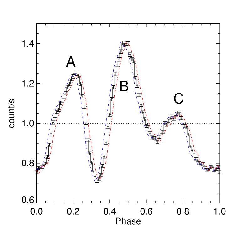
Figure 1: Phase-folded pulse profile of SMC X-3 derived from the best-fit period of 7.7720059. The profile is normalized at an average count rate of 44.49 cts s^-1. Red and blue lines correspond to the derived pulse profile for a period shifted by $\pm 5\times 10^{-5}$ s, which is $\sim$1000 times larger than the derived period uncertainty. This was chosen to demonstrate the accuracy of the derived period. Three peaks are clearly distinguished.

Figure 2: Left: Pulse profiles of SMC X-3 obtained from the EPIC-pn data in different energy bands. The profiles are background subtracted and normalized to their average count rate (from bottom to top: 4.33, 7.90, 12.6, 10.9, and 8.68 cts s^-1). Right: Hardness ratios derived from the pulse profiles in two neighboring standard energy bands as a function of pulse phase. The red horizontal lines denote the pulse-phase-averaged HR.

In Fig. 2 we present the phase-folded light curves for the five energy bands introduced above, together with the four phase-resolved hardness ratios. The hardness ratios $HR_{i}$ ($i=1,2,3,4$) are defined as

$$HR_{i}=\frac{R_{i+1}-R_{i}}{R_{i+1}+R_{i}},$$ (2)

with R_i denoting the background-subtracted count rate in the i^th energy band. The plots revealed that the prominence of the three major peaks are strongly dependent on the energy range: the pulsed emission appears to be dominated by high-energy photons (i.e., $>2$ keV), while in the softer bands, the pulse shape is less pronounced. To better visualize the spectral dependence of the pulse phase, we produced a 2D histogram for the number of events as function of energy and phase (top panel of Fig. 3). The histogram of the events covers a wide dynamic range because the efficiency of the camera and telescope varies strongly with energy. To produce an image where patterns and features (such as the peak of the pulse) are more easily recognized, we normalized the histogram by the average effective area of the detector for the given energy bin and then normalized it a second time by the phase-averaged count rate in each energy bin (middle panel, Fig. 3). Last, in the lower bin, each phase-energy bin was divided by the average soft X-ray flux (0.2-0.6 keV) of the same phase bin (bottom panel, Fig. 3). This energy range was chosen because it displays minimum phase variability (Fig. 2).

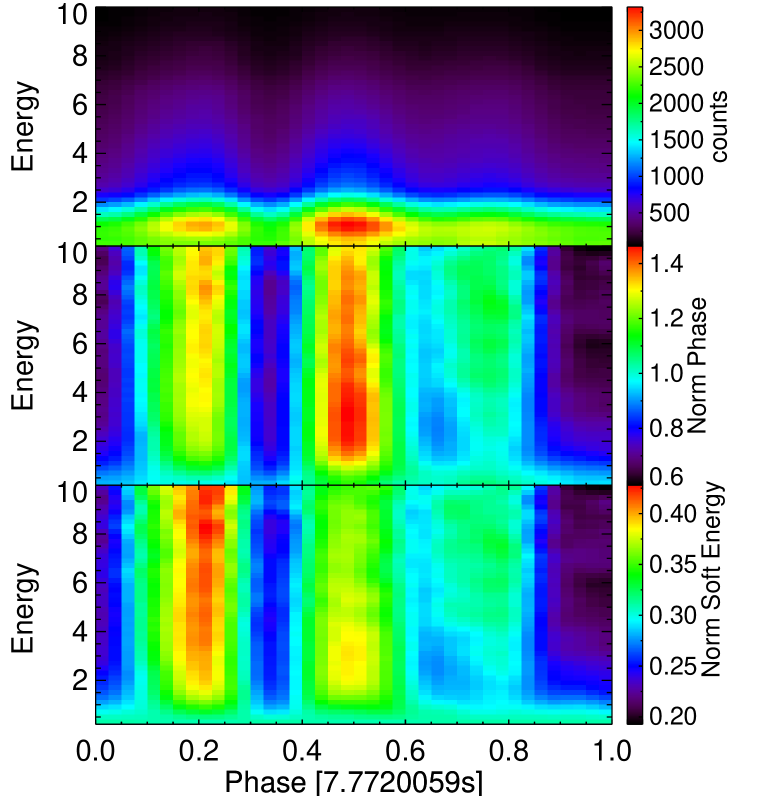
Figure 3: Phase-dependent spectral heat map, obtained by binning the EPIC-pn source counts to 40 phase and 50 energy bins. Top: Colors are proportional to the number of counts per bin. Middle: Data rates are corrected for the EPIC-pn response matrix efficiency and normalized by the phase-averaged number of counts in each energy bin. Bottom: Data normalized a second time using the rate average of each phase bin for the soft X-ray band (0.2-0.6 keV).

2.4 X-ray spectral analysis

We performed phase-averaged and phase-resolved spectroscopy of the pn data and a separate analysis of the RGS data, which was performed using the latest version of the XSPEC fitting package, Version 12.9.1 (Arnaud 1996). The spectral continuum in both phase-averaged and phased-resolved spectroscopy was modeled using a combination of an absorbed multicolor disk blackbody (MCD) and a power-law component. The interstellar absorption was modeled using the tbnew code, which is a new and improved version of the X-ray absorption model tbabs (Wilms et al. 2011). The atomic cross-sections were adopted from Verner et al. (1996). We considered a combination of Galactic foreground absorption and an additional column density accounting for both the interstellar medium of the SMC and the intrinsic absorption of the source. For the Galactic photoelectric absorption, we considered a fixed column density of nH_GAL = 7.06$\times 10^{20}$ cm⁻² (Dickey & Lockman 1990), with abundances taken from Wilms et al. (2000).

2.4.1 Phase-averaged spectroscopy

Both thermal and nonthermal emission components were required to successfully fit the spectral continuum. More specifically, when modeling the continuum using a simple power law, there was a pronounced residual structure that strongly indicated thermal emission below 1 keV. On the other hand, nonthermal emission dominated the spectrum at higher energies. The thermal emission was modeled by an MCD model (for the rationale of this choice, see the discussion in Section 4), which we modeled using the XSPEC model diskbb. The continuum emission models alone could not fit the spectrum successfully, and strong emission-like residuals were noted at ${\sim}$0.51, ${\sim}$0.97, and ${\sim}$6.63 keV and yielded a reduced $\chi^{2}$ value of 1.93 for 198 dof. (see ratio plot in Fig. 4). The corresponding emission features where modeled using Gaussian curves, yielding a $\chi^{2}$ value of 1.01 for 190 dof. The three emission lines are centered at ${\rm E_{1}}{\sim}0.51$ keV, ${\rm E_{2}}{\sim}0.96$ keV, and ${\rm E_{3}}{\sim}6.64$ keV and have equivalent width values of 6.6${}_{-4.1}^{+5.0}$ eV, 19${}_{-5.1}^{+7.0}$ eV, and 72${}_{-15}^{+17}$ eV, respectively. The ${\rm E_{2}}$ and ${\rm E_{3}}$ lines have a width of $83.8_{-2.6}^{3.0}$ eV and 361${}_{-80.1}^{+89.7}$ eV, respectively, and the ${\rm E_{1}}$ line was not resolved. The three emission-like features also appear in the two MOS detectors (see Fig. 4) and the RGS data. The emission-like features in the MOS spectra increase the robustness of their detection, but the MOS data are not considered in this analysis. The MOS1 detector was heavily piled up, and since we used the pn detector for the phase-resolved spectroscopy (as it yields more than three times the number of counts of the MOS2 detector), we also opted to exclude the MOS2 data and only use the pn data for the phase-averaged spectroscopy in order to maintain consistency. For display purposes, we show the MOS1, MOS2, and pn spectra and the data-to-model vs energy plots in Fig. 5. For the purposes of this plot, we fit the spectra of the three detectors using the diskbb plus powerlaw model, with all their parameters left free to vary. This choice allows for the visual detection of the line-like features while compensating for the considerable artificial hardening of the piled-up MOS1 detector. The MOS data indicate that the line-like features at ${\sim}0.5\,$keV and ${\sim}1\,$keV are composed of more emission lines that are unresolved by pn. This finding is confirmed by the RGS data (see Sect. 2.4.3 for more details). Narrow residual features are still present in the 1.7-2.5 kev range. They stem most likely from incorrect modeling of the Si and Au absorption in the CCD detectors by the EPIC pn calibration, which often results in emission and/or absorption features at ${\sim}$1.84 keV and ${\sim}$2.28 keV (M$\beta$) and 2.4 keV (M$\gamma$). Since the features are not too pronounced and did not affect the quality of the fit or the values of the best-fit parameters, they were ignored, but their respective energy channels were still included in our fits.

The best-fit parameters for the modeling of the phase-averaged pn data are presented in Tables 6 and 7, with the normalization parameters of the two continuum components given in terms of their relevant fluxes (calculated using the multiplicative XSPEC model cflux). The phase-averaged pn spectrum along with the data-to-model ratio plot (without the Gaussian emission lines) is presented in Figure 4. The phase-averaged spectrum was also modeled using a single-temperature blackbody instead of the MCD component. The fit was qualitatively similar to the MCD fit, with a k${\rm T_{BB}}$ temperature of 0.19$\pm 0.01$ keV, a size of 168${}_{-16.4}^{+22.1}$ km, and a power-law spectral index of $0.98\pm 0.01$.

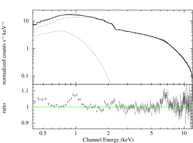
Figure 4: Phase-averaged X-ray spectrum without the Gaussian emission lines. Top plot: Normalized counts vs energy. Bottom plot: Data-to-model ratio plot.

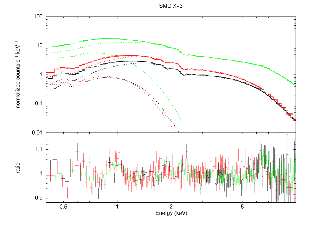
Figure 5: Phase-averaged X-ray spectrum with only the continuum model for all EPIC detectors (black: MOS1, red: MOS2, green: pn). Top plot: Normalized counts vs energy. Bottom plot: Data-to-model ratio plot.

2.4.2 Phase-resolved spectroscopy

We created separate spectra from 20 phase intervals of equal duration. We studied the resulting phase-resolved spectra by fitting each individual spectrum separately using the same model as in the phase-averaged spectrum. We noted the behavior of the two spectral components and the three emission lines, and monitored the variation of their best-fit parameters as the pulse phase evolved. The resulting best-fit values for the continuum are presented in Table 6, and those of the emission lines in Table 7. In Figure 7 we present the evolution of the different spectral parameters and the source count rate with the pulse phase.

For purposes of presentation and to further note the persistent nature of the soft emission, we also fit all 20 spectra simultaneously and tied the parameters of the thermal component, while the parameters of the power-law component were left free to vary. The results of this analysis were qualitatively similar to the independent spectral fitting (see Fig. 6, where the spectral evolution of the source is illustrated). Nevertheless, the decision to freeze the temperature and normalization of the soft component at the phase-averaged best-fit value introduces bias to our fit, and we therefore only tabulate and study the best-fit values for the independent modeling of the phase-resolved spectra.

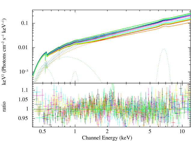
Figure 6: Spectral model and data-to-ratio plot of the simultaneous fit of the 20 phase-resolved spectra

Figure 7: Evolution of spectral parameters (Table 6) for the phase-resolved spectroscopy presented in Sect. 2.4.2. The arrow represents the upper limit for the flux of the MCD component for phase-resolved spectrum 5. The corresponding temperature was frozen to the phase-averaged value (see the first row of Table 6).

2.4.3 RGS spectroscopy

The RGS spectra were not grouped and were fitted employing Cash statistics (Cash 1979) and with the same continuum model as the phased-averaged pn spectra. The model yielded an acceptable fit, with a reduced $\chi^{2}$ value of 1.05 for 1875 dof. The RGS spectra were also fitted simultaneously with the pn phase-averaged spectra (with the addition of a normalization constant, which was left free to vary) yielding best-fit parameter values consistent within 1 ${\sigma}$ error bars with the pn continuum model. We therefore froze the continuum parameters to the values tabulated in the first row of Table 6. We note that a simple absorbed power-law model still describes the continuum with sufficient accuracy, and the use of a second component only improves the fit by $\sim$2.7$\sigma,$ as indicated by performing an ftest.

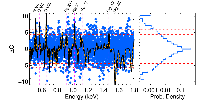
Figure 8: Emission and absorption lines detected in the RGS data. Left plot: ${\Delta}$C for each line vs energy. Black corresponds to Gaussians with 2 eV width and orange to a width of 10 eV. The blue points correspond to the simulated spectra of the model continuum. Right plot: Probability density function for ${\Delta}$C values for the simulated spectra. The dashed line corresponds to three standard deviations assuming that the probability density function follows the Gaussian distribution. The dotted line encloses 99.7% of the ${\Delta}$C values.

We searched the RGS spectra for emission and absorption lines by a blind search for Gaussian features with a fixed width. The spectrum was searched by adding the Gaussian to the continuum and fitting the spectrum with a step of 10 eV, and the resulting $\Delta$C was estimated for each step. Emission and absorption lines are detected with a significance higher than 3${\sigma.}$ To estimate the values for the $\Delta$C that correspond to the 3$\sigma$ significance, we followed a similar approach as Kosec et al. (2018). We simulated 1000 spectra based on the continuum model and repeated the process of line-search using the fixed-width Gaussian. We plot the probability distribution of the $\Delta$C values and indicate the range of $\Delta$C values within which lies the 99.7% of the trials. $\Delta$C values outside this interval (see Fig. 8, dotted lines) are defined as having a 3$\sigma$ significance. In Fig. 8 we plot the $\Delta$C improvement of emission and absorption lines detected in the RGS data assuming Gaussian lines with a fixed width of 2 eV (black solid line) and 10 eV (orange dashed line). The line significance is affected by the width of the Gaussian, and a more thorough approach should include a grid of different line widths in order to achieve the best fit. We here used the emission lines with a significance higher than 3 $\sigma$ (dotted line) assuming a 2 eV fixed width, which were then fit manually with the width as a free parameter. The best-fit values are presented in Table 8. We also note a strong absorption line at more than 5 $\sigma$ significance and several tentative others. The most prominent absorption line is centered at ${\approx}1.585\,$keV. When the line is associated with MgXII absorption, it appears to be blueshifted by 7%. The apparent blueshift could be an indication of outflows, but he velocity appears to be considerable lower than the velocities inferred for ULXs (e.g., Pinto et al. 2016). A more thorough study of the RGS data using an extended grid of all line parameters will be part of a separate publication.

Table 1: Best-fit parameters for the continuum for the 20 phases and the phase-averaged spectrum. All errors are in the 90% confidence range.

Phase	nH [a]	k${\rm T_{\rm soft}}$	Fsoft [b]	${\Gamma}$	FPO [c]	count-rate	$\chi^{2}/dof$
	[$\times 10^{21}$ cm2]	keV	$10^{-11}{\rm erg\,cm^{-2}\,s^{-1}}$		$10^{-11}{\rm erg\,cm^{-2}\,s^{-1}}$	cts/s
Average	1.36${}_{-0.62}^{+0.13}$	0.24${}_{-0.03}^{+0.04}$	1.44${\pm 0.19}$	0.98${\pm 0.10}$	29.8$\pm 0.95$	41.8$\pm 0.04$	1.01/190
0	1.50${}_{-0.39}^{+0.53}$	0.30$\pm 0.03$	1.17${\pm 0.30}$	0.92${}_{-0.03}^{+0.02}$	40.1${\pm 0.37}$	52.5$\pm 0.19$	1.05/181
1	1.14${}_{-0.26}^{+0.33}$	0.40${}_{-0.06}^{+0.07}$	1.70${\pm 0.25}$	0.90$\pm 0.04$	27.8${\pm 0.29}$	39.9$\pm 0.17$	0.95/177
2	1.38${}_{-0.33}^{+0.41}$	0.21${}_{-0.03}^{+0.04}$	1.66${\pm 0.60}$	1.04$\pm 0.03$	20.1${\pm 0.25}$	30.6$\pm 0.17$	1.01/169
3	1.82${}_{-0.49}^{+0.55}$	0.20${}_{-0.03}^{+0.04}$	2.02${\pm 0.74}$	1.03$\pm 0.02$	26.4${\pm 0.28}$	37.8$\pm 0.17$	1.03/171
4	1.76${}_{-0.44}^{+0.75}$	0.24${}_{-0.04}^{+0.08}$	1.41${\pm 0.50}$	1.00$\pm 0.02$	38.9${\pm 0.35}$	52.7$\pm 0.21$	1.00/183
5	0.96${}_{-0.10}^{+0.11}$	–	$<$2.17	1.01$\pm 0.01$	44.6${\pm 0.90}$	59.9$\pm 0.20$	0.87/184
6	1.45${}_{-0.28}^{+0.35}$	0.20${}_{-0.03}^{+0.05}$	1.28${\pm 0.87}$	1.01$\pm 0.02$	41.0${\pm 0.35}$	55.3$\pm 0.19$	1.01/187
7	1.21${}_{-0.22}^{+0.25}$	0.26${}_{-0.04}^{+0.06}$	1.25${\pm 0.38}$	1.01$\pm 0.02$	32.1${\pm 0.37}$	45.6$\pm 0.20$	0.89/182
8	1.32${}_{-0.20}^{+0.22}$	0.28$\pm 0.03$	2.14${\pm 0.30}$	0.95$\pm 0.03$	27.1${\pm 0.34}$	39.7$\pm 0.17$	0.81/178
9	1.27${}_{-0.25}^{+0.28}$	0.23$\pm 0.03$	2.13${\pm 0.48}$	0.92$\pm 0.03$	28.6${\pm 0.40}$	40.2$\pm 0.17$	0.88/178
10	1.66${}_{-0.41}^{+0.49}$	0.26$\pm 0.03$	2.48${\pm 0.63}$	0.88${}_{-0.03}^{+0.02}$	31.5${\pm 0.28}$	42.9$\pm 0.18$	0.87/182
11	1.84${}_{-0.44}^{+0.58}$	0.22$\pm 0.03$	2.21${\pm 0.94}$	0.94$\pm 0.04$	32.0${\pm 0.46}$	43.8$\pm 0.18$	1.08/178
12	1.63${}_{-0.48}^{+0.63}$	0.21${}_{-0.03}^{+0.04}$	2.24${\pm 1.11}$	0.97$\pm 0.03$	27.7${\pm 0.37}$	39.5$\pm 0.17$	1.09/173
13	1.23${}_{-0.23}^{+0.26}$	0.26${}_{-0.03}^{+0.04}$	1.83${\pm 0.35}$	1.05$\pm 0.03$	21.8${\pm 0.26}$	34.1$\pm 0.17$	0.99/173
14	1.57${}_{-0.35}^{+0.48}$	0.25${}_{-0.04}^{+0.05}$	2.04${\pm 0.35}$	1.14${}_{-0.04}^{+0.03}$	20.0${\pm 0.25}$	32.4$\pm 0.15$	0.89/170
15	1.31${}_{-0.25}^{+0.28}$	0.25${}_{-0.03}^{+0.04}$	1.68${\pm 0.38}$	1.10${}_{-0.04}^{+0.03}$	20.3${\pm 0.25}$	31.9$\pm 0.15$	1.07/170
16	1.12${}_{-0.22}^{+0.26}$	0.27$\pm 0.05$	0.15${\pm 0.31}$	1.06${}_{-0.04}^{+0.06}$	20.9${\pm 0.26}$	32.5$\pm 0.15$	1.01/172
17	1.43${}_{-0.24}^{+0.27}$	0.24$\pm 0.03$	1.85${\pm 0.39}$	0.91$\pm 0.02$	29.0${\pm 0.31}$	39.5$\pm 0.17$	0.94/187
18	1.79${}_{-0.36}^{+0.54}$	0.21${}_{-0.03}^{+0.04}$	1.77${\pm 0.82}$	0.96$\pm 0.02$	34.9${\pm 0.33}$	46.6$\pm 0.18$	1.11/178
19	2.26${}_{-0.55}^{+0.68}$	0.22${}_{-0.03}^{+0.05}$	2.17${\pm 0.61}$	0.95$\pm 0.02$	39.8${\pm 0.36}$	51.5$\pm 0.19$	0.96/182

Table 2: Bestfit parameters for the emission lines for the 20 phases. All errors are in the 90% confidence range.

Phase	${\rm E_{1}}$	${\rm K_{1}}$	${\rm E_{2}}$	${\rm K_{3}}$	${\rm E_{3}}$	${\rm{\sigma}_{3}}$	${\rm K_{3}}$
	keV	$10^{-4}$ cts cm-2 s-1	keV	$10^{-4}$ cts cm-2 s-1	keV	keV	$10^{-4}$ cts cm-2 s-1
Averagea	0.51$\pm 0.02$	3.02${}_{-1.78}^{+2.36}$	0.96$\pm 0.02$	3.55${}_{-0.98}^{+1.32}$	6.64${}_{-0.15}^{+0.16}$	0.36${}_{-0.08}^{+0.09}$	1.70${}_{-0.35}^{+0.39}$
0	0.49$\pm 0.03$	11.2${}_{-8.52}^{+15.8}$	0.98$\pm 0.03$	2.79${}_{-1.19}^{+1.18}$	6.76${}_{-0.15}^{+0.16}$	0.25${}_{-0.15}^{+0.20}$	2.43${}_{-1.23}^{+1.40}$
1	0.51${}_{-0.03}^{+0.04}$	6.98${}_{-5.27}^{+8.06}$	0.94${}_{-0.05}^{+0.06}$	1.91$\pm{1.13}$	6.44${}_{-0.32}^{+0.20}$	$<0.39$	1.33${}_{-0.82}^{+0.96}$
2	0.53${}_{-0.15}^{+0.09}$	$<$10.8	1.02${}_{-0.03}^{+0.02}$	2.69${}_{-0.89}^{+0.97}$	6.76${}_{-0.30}^{+0.26}$	0.45*	2.28${}_{-1.15}^{+1.10}$
3	0.50${}_{-0.05}^{+0.06}$	$<$21.9	0.97$\pm 0.03$	2.75${}_{-1.16}^{+1.19}$	6.49${}_{-0.26}^{+0.14}$	$<0.48$	0.92${}_{-0.62}^{+1.13}$
4	0.48${}_{-0.02}^{+0.03}$	16.8${}_{-12.5}^{+23.5}$	–	–	–	–	–
5	0.55${}_{-0.04}^{+0.08}$	4.96${}_{-4.31}^{+5.21}$	0.98$\pm 0.03$	3.12$\pm{1.13}$	6.61${}_{-0.30}^{+0.26}$	0.41${}_{-0.22}^{+0.34}$	3.06${}_{-1.53}^{+2.08}$
6	–	–	–	–	–	–	–
7	–	–	0.94$\pm 0.03$	2.69$\pm{1.23}$	–	–	–
8	–	–	–	–	6.74${}_{-0.24}^{+0.22}$	0.28${}_{-0.24}^{+0.38}$	1.80${}_{-1.07}^{+1.54}$
9	–	–	0.98${}_{-0.02}^{+0.03}$	3.09${}_{-1.08}^{+1.10}$	6.81${}_{-0.28}^{+0.31}$	0.45*	2.93$\pm{1.13}$
10	0.46$\pm 0.04$	16.0${}_{-13.1}^{+21.9}$	–	–	–	–	–
11	0.50${}_{-0.02}^{+0.03}$	14.7${}_{-10.6}^{+20.2}$	0.94$\pm 0.03$	3.12$\pm{1.17}$	6.76${}_{-0.39}^{+0.29}$	0.45*	2.97${}_{-1.30}^{+1.29}$
12	0.46${}_{-0.04}^{+0.03}$	$<$8.90	0.97$\pm 0.03$	2.30${}_{-1.13}^{+1.14}$	6.70${}_{-0.19}^{+0.20}$	0.45*	3.60${}_{-1.41}^{+1.25}$
13	–	–	0.96${}_{-0.09}^{+0.05}$	1.70${}_{-1.06}^{+1.07}$	–	–	–
14	0.51${}_{-0.05}^{+0.08}$	7.49${}_{-6.58}^{+14.1}$	0.99${}_{-0.04}^{+0.03}$	1.85${}_{-1.03}^{+1.04}$	6.9*	0.44${}_{-0.16}^{+0.20}$	2.52${}_{-1.14}^{+1.25}$
15	–	–	0.95${}_{-0.07}^{+0.16}$	1.13${}_{-1.04}^{+1.06}$	6.87${}_{-0.15}^{+0.19}$	0.30${}_{-0.12}^{+0.22}$	2.32${}_{-0.93}^{+1.04}$
16	–	–	1.02${}_{-0.08}^{+0.04}$	1.76${}_{-0.93}^{+0.94}$	6.42${}_{-0.19}^{+0.42}$	0.30${}_{-0.14}^{+0.39}$	1.79${}_{-0.90}^{+1.50}$
17	–	–	–	–	6.58${}_{-0.11}^{+0.12}$	$<0.29$	1.67${}_{-0.87}^{+0.90}$
18	0.53$\pm 0.03$	6.41${}_{-5.31}^{+5.44}$	1.00${}_{-0.04}^{+0.03}$	2.25${}_{-1.17}^{+1.12}$	6.45$\pm 0.06$	$<0.14$	1.06$\pm{0.53}$
19	0.49$\pm 0.02$	24.2${}_{-16.0}^{+29.6}$	–	–	6.60${}_{-0.36}^{+0.13}$	$<0.60$	1.38${}_{-0.91}^{+1.88}$

Table 3: RGS emission lines and the corresponding the $\Delta$C value for each added Gaussian. All errors are in the 90% confidence range.

Linea	${\rm E}$	${\rm{\sigma}}$	${\rm norm}$	${\Delta}$C
eV	keV	eV	$10^{-4}$ cts cm-2 s-1
N VII (500.3)	0.512${}_{-0.014}^{+0.011}$	16.02${}_{-6.44}^{+13.00}$	3.152${}_{-1.506}^{+1.510}$	12.5
O VII (561-574)	0.571$\pm 0.005$	$<10.01$	1.341${}_{-0.893}^{+0.901}$	7.29
O VIII (653.6)	0.657${}_{-0.03}^{+0.003}$	$<7.0$	0.6${}_{-0.3}^{+0.5}$	14.9
Fe XIX-XXI(917.2)	0.923$\pm 0.006$	10.40${}_{-3.39}^{+6.73}$	0.964${}_{-0.371}^{+0.377}$	20.3
Ne X (1022)	1.025${}_{-0.002}^{+0.003}$	3.481${}_{-2.017}^{+15.09}$	0.653${}_{-0.246}^{+0.247}$	20.6
Fe XXIII-XXIV (1125)	1.125${}_{-0.020}^{+0.018}$	16.77${}_{-11.55}^{+24.61}$	0.597$\pm 0.413$	5.8

2.5 X-ray spectral and temporal evolution during the 2016 outburst

We report on the long-term evolution of the values of the PF and HR throughout the 2016 outburst, using the data from Swift observatory. Using the method described in Sect. 2.3, we searched for the pulse period of SMC X-3 for all the analyzed Swift/XRT observations using the barycenter corrected events within the 0.5-10.0 keV energy band. The resulting pulse periods are presented in Fig. 9. Using the derived best-fit periods, we estimated the PF for all the Swift/XRT observations (see Fig. 10). From the extracted event files, we calculated the phase-average hardness ratios for all Swift/XRT observations. For simplicity and in order to increase statistics, we used three energy bands to estimate two HR values: HR soft, using the 0.5-2.0 keV and 2.0-4.5 keV bands, and HR hard, using the 2.0-4.5 keV and 4.5-10.0 keV bands.

We performed the same calculations for the phase-resolved spectrum of SMC X-3 as measured by the XMM-Newton ToO. In particular, we estimated the above two HR values for 40 phase intervals. The evolution of the spectral state of SMC X-3 with time and pulse phase as depicted by these two HR values is shown in Fig. 11 (left). For comparison, we have plot in parallel (Fig. 11, right panel) the evolution of the HR with NS spin phase during the XMM-Newton observation. We note that although quantitatively different HR values are expected for different instruments (i.e., Swift/XRT and XMM-Newton/EPIC-pn), a qualitative comparison of the HR evolution can be drawn. More specifically, the left-hand plot probes the long-term HR evolution versus the mass accretion rate (inferred from the registered source count-rate), and the right-hand side shows the HR evolution with pulse phase.

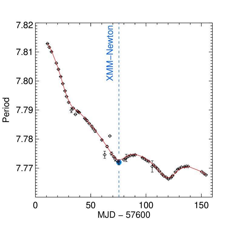
Figure 9: Pulse period evolution during the 2016 burst of SMC X-3 based on the analysis of Swift/XRT data. The red line is based on the best-fit model describing the evolution of the spin (Townsend et al. 2017). The date of the XMM-Newton pointing is marked by the blue dashed vertical line. The spin period derived by the EPIC-pn data is marked with a blue circle. This solution coincides with the one derived from Swift/XRT on an observation performed within the same day.

Figure 10: PF: Pulsed fraction defined in equation 1. Swift errors are computed based on the Poisson uncertainty of the pulse profile and do not include calculations based on the period uncertainties, as a systematic uncertainty of 0.01 was added to the estimated Swift/XRT PF. The XMM-Newton PF is estimated from the profile presented in Fig. 1, and errors are estimated from the 1$\sigma$ error in the derived period.

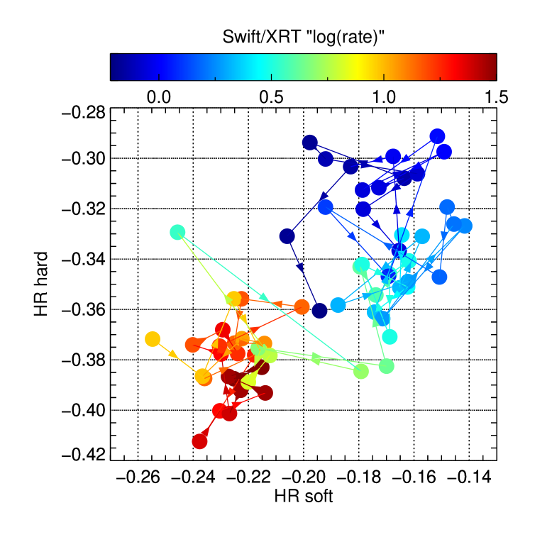
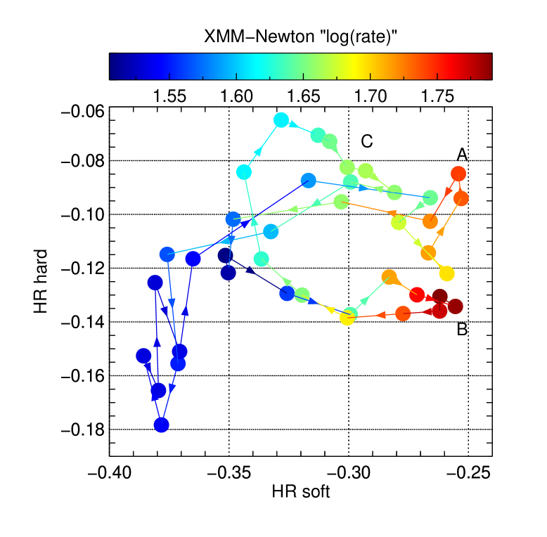
Figure 11: Left: Hardness ratio evolution of the average X-ray spectrum of SMC X-3 as estimated for all Swift/XRT observations. Calculations were made using the three bands 0.5-2.0 keV, 2.0-4.5 keV, and 4.5-10.0 keV. HR soft was estimated using the two former energy bands, while HR hard was estimated for the latter two. Colors are representative of the average count rate of each observation, while arrows connect the observations in chronological order. Right: Hardness ratio evolution of the phase-resolved X-ray spectrum of SMC X-3 based on the XMM-Newton observation. HRs were defined as in the left plot, while 40 phase bins were used. Colors are representative of the average count rate of each phase bin, while arrows connect the observations based on their phase evolution. The labels A, B, and C represent the three peaks in Fig. 1.

3 Emission pattern, pulse reprocessing, and the observed PF

To investigate the evolution of the PF with luminosity and to investigate the origin of the soft excess as determined from the phase-resolved analysis, we constructed a toy model for the beamed emission. The model assumes that the primary beamed emission of the accretion column is emitted perpendicularly to the magnetic field axis, in a fan-beam pattern (Basko & Sunyaev 1976). Furthermore, it is assumed that all the emission originates in a point source at a height of ${\sim}2-3\,$km from the surface of the NS. A fraction of the fan emission will also be beamed toward the NS surface, off of which it will be reflected, resulting in a secondary polar beam that is directed perpendicularly to the fan beam (this setup is described in Trümper et al. 2013, see also their Fig. 4 ). Partial beaming of the primary fan emission toward the NS surface is expected to occur primarily as a result of scattering by fast electrons at the edge of accretion column (Kaminker et al. 1976; Lyubarskii & Syunyaev 1988; Poutanen et al. 2013), and to a lesser degree as a result of gravitational bending of the fan-beam emission. The latter may also result in the emission of the far-away pole entering the observer line of sight. In the model, gravitational bending is accounted for according to the predictions of Beloborodov (2002).

The size of the accretion column (and hence the height of the origin of the fan-beam emission) is a function of the NS surface magnetic field strength and the mass accretion rate (see Mushtukov et al. 2015, and references within). As it changes, it affects the size of the illuminated region on the NS surface and therefore the strength of the reflected polar emission. If the accretion rate drops below the critical limit, the accretion column becomes optically thin in the direction parallel to the magnetic field axis, and the primary emission is then described by the pencil-beam pattern Basko & Sunyaev (1975). In principle, the polar and pencil-beam emission patterns can be phenomenologically described by the same algebraic model. We also modeled the irradiation of any slab or structure (e.g., the inner part of the accretion disk that is located close to the NS) by the combined beams. Last, while arc-like accretion columns and hot-spots have been found in 3D magnetohydrodynamic simulations (Romanova et al. 2004) of accreting pulsars, we did not include them in our treatment as they would merely introduce an anisotropy in the pulse profile and not significantly affect our results.

3.1 Pulsed fraction evolution

The beaming functions of the polar and fan beams are given by $f\sin^{m}{\phi}$ and $p\cos^{k}{\phi}$, respectively. Here $\phi$ is the angle between the magnetic field axis and the photon propagation and is thus a function of the angle between the magnetic and rotation axis ($\theta$), the angle of the NS rotation axis, the observing angle ($i$), and the NS spin phase. The exponent values $m$ and $k$ can be as low as 1, but in the general case of the accretion column emission, they can have significantly higher values (Trümper et al. 2013). We constructed various pulse profiles for different combinations of fan- and polar-beam emission patterns with different relative intensities of the fan and polar beams (i.e., $F_{\rm Polar}/F_{\rm Fan}$ ranging from $\sim$0.01 to ${\sim}30$). We note that these values exceed any realistic configuration between the fan beam and the reflected polar beam. More specifically, since the polar beam is a result of reflection of the fan beam, it is only for a very limited range of observing angles that its contribution will (seemingly) exceed that of the fan beam, and thus a value of $F_{\rm Polar}/F_{\rm Fan}\gtrsim 2$, is unlikely. On the other hand, the increasing height of the emitting region, which would result in a smaller fraction of the fan beam being reflected by the NS surface, is limited to $\lesssim 10\,km$ (Mushtukov et al. 2015), thus limiting the $F_{\rm Polar}/F_{\rm Fan}$ ratio to values greater than 0.1 (see, e.g., Fig 2. of Poutanen et al. 2013). Despite these physical limitations, we have extended our estimates to these exaggerated values in order to better illustrate the contribution of each component (fan and polar) to the PF. Moreover, a value of $F_{\rm Polar}/F_{\rm Fan}$ exceeding 10 qualitatively describes the pencil-beam regime, which is expected at lower accretion rates. We estimated the PF for a range of observer angles and for different combinations of angles between the magnetic and rotation axis. An indicative result for a 45^o angle between the NS magnetic field and rotation axis and for an $r_{G}/r_{NS}=0.25$ is plotted in Fig 12.

3.2 Reprocessed radiation

To investigate the origin of the soft excess (i.e., the thermal component in the spectral fits) and to assess its contribution to the pulsed emission, we studied the pattern of the reprocessed emission from irradiated optically thick material in the vicinity of the magnetosphere. More specifically, we considered a cylindrical reprocessing region that extends symmetrically above and below the equatorial plane. The radius of the cylinder is taken to be equal to the magnetospheric radius, where the accretion disk is interrupted. The latitudinal size of the reprocessing region corresponds to an angular size of 10^o, as viewed from the center of the accretor (see, e.g., Hickox et al. 2004, and our Fig. 16 for an illustration). The model takes into account irradiation of this region by the combined polar- and fan-beam emission. If d is the unit vector toward the observer and n is the disk surface normal, the total radiative flux that the observer sees would be estimated from their angle d${\cdot}$n. We furthermor assume that the observer sees only half of the reprocessing region (and disk, i.e., $\pi$). Light-travel effects of the scattered/reprocessed radiation (e.g., equation 3 of Vasilopoulos & Petropoulou 2016) should have a negligible effect in altering the phase of the reprocessed emission, as the light-crossing time of the disk is less than 1% (0.05% $=(1000km/c)/P_{NS}*100\%$) of the NS spin period. Thus, any time lag that is expected should be similar in timescale to the reverberation lag observed in LMXB systems (e.g., H1743-322: De Marco & Ponti 2016).

To determine the fraction of the pulsed emission that illuminates the reprocessing region, we integrated the emission over the 10^o angular size of the reprocessing region and estimated the PF for an inclination angle between the rotational and the magnetic filed axes ($\theta$) that ranges between 0^o and 90^o (Fig. 13, dotted line). We also estimate the PF originating from the reprocessing region assuming a ratio of $F_{\rm Polar}/F_{\rm Fan}=$0.25 (Fig. 13, solid line). To further probe the contribution of the two beam components to the reprocessed emission, we estimated the PF for two extreme cases in which all the primary emission is emitted in the polar beam (Fig. 13, green dashed line) or only the fan beam (Fig. 13, blue dashed line). As we discussed, this scenario is unrealistic, since the polar beam is the result of reflection of the fan beam. However, this setup would adequately describe the pencil-beam emission, expected at lower accretion rates (e.g., Basko & Sunyaev 1975).

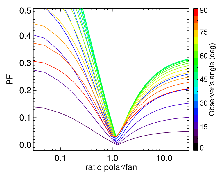
Figure 12: PF versus intensity between fan and pencil beam.

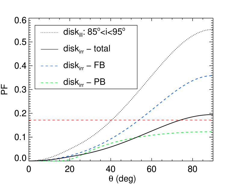
Figure 13: PF of the reprocessed emission of a fan-beam pattern for various inclination angles between the magnetic and rotation axis. The dotted line represents the PF of the integrated emission over a cylindrical surface of angular size of 10^o and located at the equatorial plane of the NS. The solid line is the calculated reprocessed PF for a combination of polar beam and fan beam ($F_{\rm Polar}/F_{\rm Fan}=$0.25). The dashed blue and green lines show the PF of reprocessed emission that would originate from a pure fan-beam and polar-beam illuminating pattern, respectively. The red horizontal line represents the limit on the PF given the variability of the observed flux of the thermal component, presented in Figure 7.

Figure 14: Absorption-corrected PL X-ray luminosity vs bolometric disk-BB luminosity. No clear correlation between the two quantities was established.

4 Discussion

The high quality of the XMM-Newton spectrum of SMC-X3 and the very large number of total registered counts have allowed us to perform a detailed time-resolved spectroscopy where we robustly constrained the different emission components and monitored their evolution with pulse phase. Furthermore, the high time-resolution of the XMM-Newton detectors, complimented with the numerous Swift/XRT observations (conducted throughout the outburst), have allowed for a detailed study of the long- and short-term temporal behavior of the source. Below, we present our findings and their implications with regard to the underlying physical mechanisms that are responsible for the observed characteristics.

4.1 Emission pattern of the accretion column and its evolution

The 0.01-12 keV luminosity of SMC X-3 during the XMM-Newton observation is estimated at 1.45$\pm 0.01\times 10^{38}$ erg/s for a distance of ${\sim}$62 kpc. The corresponding mass accretion rate, assuming an efficiency of $\xi=0.21$ (e.g., Sibgatullin & Sunyaev 2000), is ${\dot{M}}{\sim}1.2\times 10^{-8}\,{M_{\odot}}/{\rm yr}$, which places the source well within the fan-beam regime (Basko & Sunyaev 1976; Nagel 1981). Furthermore, the shape of the pulse profile (Fig. 1) indicates a more complex emission pattern, comprised of the primary fan beam and a secondary reflected polar beam, as was proposed in Trümper et al. (2013) and briefly presented in Section 3. The energy-resolved pulse profiles and the phase-resolved hardness ratios presented in Fig. 2 strongly indicate that the pulsed emission is dominated by hard-energy photons, while the smooth single-color appearance of the 0.2-0.6 keV energy range in the lower bin heat map presented in Fig. 3 indicates a soft spectral component that does not pulsate.

Using our toy-model for the emission of the accretion column, we were able to explore the evolution of the PF with the $F_{\rm Polar}/F_{\rm Fan}$ ratio, assuming a broad range of observer viewing angles. Interestingly, the resulting PF vs $F_{\rm Polar}/F_{\rm Fan}$ ratio (Fig. 12) qualitatively resembles the evolution of the PF, with increasing source count-rate, as presented in Fig. 10, using Swift/XRT data. Following the paradigm of Basko & Sunyaev (1975) and Basko & Sunyaev (1976), we expect the emission pattern of the accretion column to shift from a pencil- to a fan-beam pattern as the accretion rate increases. Below $\sim$1 cts/sec, the emission is dominated by the pencil beam (which is qualitatively similar to the polar beam). This regime is defined by $F_{\rm Polar}/F_{\rm Fan}>2$. As the luminosity increases, the radiation of the accretion column starts to be emitted in a fan beam, which is accompanied by the secondary polar beam, corresponding to $0.7{\lesssim}F_{\rm Polar}/F_{\rm Fan}{\lesssim}2$ (this only refers to the X-axis of Fig. 10 and does not imply chronological order, which is indicated with arrows in Fig. 11). This is the era during which the XMM-Newton observation was conducted. As the accretion rate continued to increase, the accretion column grew larger, the height of the emitting region increased, and the emission started to become dominated by the fan beam as the reflected component decreases, yielding a lower value of the $F_{\rm Polar}/F_{\rm Fan}$ ratio. Nevertheless, it is evident from Fig. 10 that the PF does not readily increase as the fan beam becomes more predominant (i.e., above ${\sim}7$ cts/s). This indicates that the height of the accretion column is limited to moderate values (e.g., as argued by Poutanen et al. 2013; Mushtukov et al. 2015), and therefore a considerable contribution from the polar beam is always present.

The presence of the polar beam is also indicated by the shape of the pulse profile and its evolution during different energy bands and HR values (Figures 1 and 2). The pulse profile has three distinct peaks that we label A, B, and C from left to right in Fig. 1. The energy and HR-resolved pulse profiles presented in Fig. 2 reveal that the pulse peaks are dominated by harder emission. A closer inspection indicates that peak B is softer than the other two peaks and is still present (although much weaker) in the lower energy bands (Fig. 2, lower left bin). This finding is further supported by our study of the HR evolution of the sources throughout the XMM-Newton observation, presented in Fig. 11 (right panel). This representation clearly shows that the source is harder during high-flux intervals (the peaks of the pulse profile), but also that peak B is distinctly softer than peaks A and C. We argue that these findings indicate a different origin of the three peaks. More specifically, we surmise that the softer and more prominent peak B originates mostly from the fan beam, while the two harder peaks (A and C) are dominated by the polar-beam emission, which is expected to be harder than the fan beam. This is because only the harder incident photons (of the fan beam) will be reflected (i.e., backscattered) off the NS atmosphere, while the softer photons will be absorbed (e.g., Trümper et al. 2013; Postnov et al. 2015).

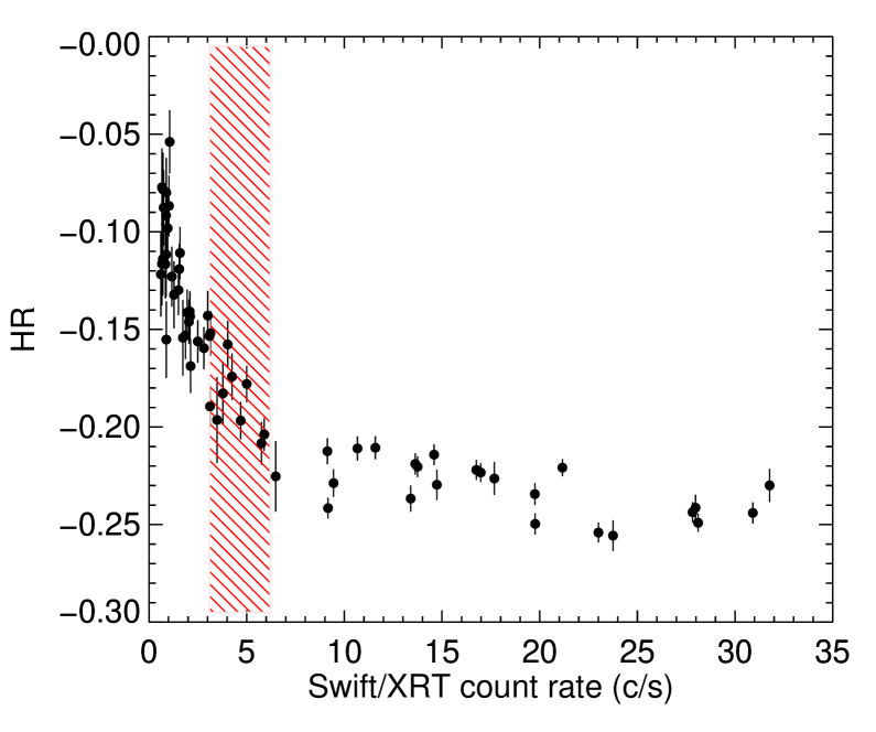
Figure 15: Hardness ratio of the 1-3 keV to 3-10 keV bands vs count rate for the Swift observations of SMX X-3 between MJDs 57611 and 57754. The red-striped area denotes the luminosity correspoding to 1-2 Eddington rates (0.3-10 keV).

The analysis of the Swift data taken throughout the outburst allowed us to also probe the long-term spectral evolution of the source. In the left panel of Fig. 11 we present the HR ratio evolution of the source throughout the 2016 outburst. Unlike the short-term evolution of the source, during which the emission is harder during the high-flux peaks of the pulses (see the data from the XMM-Newton observation presented in the right panel of Fig. 11), the emission of SMC X-3 becomes softer in the long term as the luminosity of the source increases (color-coded count rate in Fig. 11). This behavior is also evident in Fig. 15, where the HR ratio of the 1-3 keV to the 3-10 keV band is plotted versus the source count-rate. The source becomes clearly softer as the accretion rate (which corresponds to the observed flux) increases. Long-term observations of numerous XRPs suggests that they can be divided into two groups, based on their long-term spectral variability. Sources in group 1 (e.g., 4U 0115+63) exhibit a positive correlation between source hardness and its flux, while sources in group 2 (e.g., Her X-1 or this source) a negative (e.g., Tsygankov et al. 2007, 2010; Vasco et al. 2011; Klochkov et al. 2011).

It can be argued that the apparent two populations are just the result of observing the XRPs in two different regimes of mass accretion rates. At low accretion rates, deceleration of the in-falling particles in the accretion column occurs primarily via Coulomb interactions, while in the high-rate regime, the mass is decelerated through pressure from the strong radiation field (e.g., Basko & Sunyaev 1976; Wang & Frank 1981; Mushtukov et al. 2015). As the mass accretion rate increases, so does the height of the accretion column, and therefore the reflected fraction (i.e., the polar beam) starts to decrease. As the polar emission is harder than the fan beam, the total registered spectrum stops hardening and even becomes moderately softer (Postnov et al. 2015). Observationally, the positive correlation is expected at luminosities below a critical value and the negative above it. This critical value is theoretically predicted at ${\sim}1-7\times 10^{37}$ erg/s (e.g., Staubert et al. 2007; Klochkov et al. 2011; Becker et al. 2012; Postnov et al. 2015), which is in agreement with the earlier prediction of Basko & Sunyaev (1976). Observations of XRPs at different luminosities indeed show that a single source can exhibit the behavior of both groups when monitored above or below this critical value (e.g., Postnov et al. 2015).

The high-luminosity regime, which is the only regime probed by the Swift data points in Fig. 15, is essentially the diagonal branch of the hardness-intensity diagrams presented by Reig & Nespoli (2013). The source behavior, presented in Fig. 15, is consistent with the theoretical predictions for sources accreting above the critical luminosity of ${\sim}10^{37}$ erg/s. However, while the previous observations by Klochkov et al. (2011) and Postnov et al. (2015) showed the pause in the hardening of the source with increasing luminosity, and (in some sources) the slight decrease in hardness, this drop is clearly demonstrated here thanks to the numerous high-quality observations provided by the Swift telescope. Furthermore, our analysis indicates the presence of perhaps a third branch that appears when the source luminosity exceeds ${\sim}4{\times}L_{\rm Edd}$ , in which the source luminosity increases but the emission does not become softer. If this additional branch is indeed real, it may have eluded detection by Reig & Nespoli simply because the sources studied there never reached such high luminosities. It is plausible that the stabilization of the source hardness is a manifestation of the predicted physical limitations imposed on the maximum height of the accretion column (e.g., Poutanen et al. 2013; Mushtukov et al. 2015).

4.2 Origin of the soft excess and the optically thin emission

The phase-averaged spectral continuum of SMC X-3 during the XMM-Newton observation is described by a combination of a emission in the shape of a hard power-law and a softer thermal component with a temperature of ${\sim}0.24$ keV. The nonthermal component is consistent with emission from the accretion column (e.g., Becker & Wolff 2007), but the origin of the soft thermal emission is less clear. Assuming that the accretion disk is truncated approximately at the magnetosphere, and for an estimated magnetic field of ${\sim}2-3\times 10^{12}$ G (Klus et al. 2014; Tsygankov et al. 2017), the maximum effective temperature of the accretion disk would lie in the far-UV range (20-30 eV) for ${\dot{M}}{\sim}1.2\times 10^{-8}\,{M_{\odot}}/{\rm yr}$, as inferred from the observed luminosity and for $R_{\rm in}=0.5-1\,R_{\rm mag}$. Although we can exclude a typical thin disk as the origin of the emission, an inflated disk that is irradiated from the NS might be the origin of the thermal emission, because such a disk can reach higher temperatures (see, e.g., Chashkina et al. 2017, and the discussion below).

The emission is also unlikely to originate in hot plasma on the surface of the NS, as the size of a blackbody-emitting sphere that successfully fits the data is an order of magnitude larger (${\sim}170$ km) than the ${\sim 12}$ km radius of a 1.4 ${M_{\odot}}$ NS. The observed thermal emission could be the result of reprocessing of the primary emission by optically thick material that lies at a distance from the NS and is large enough to partially cover the primary emitting region (i.e., the accretion column). If a significant fraction of the primary emission is reprocessed, then this optically thick region will emit thermal radiation at the observed temperatures. A detailed description of this configuration is presented in Endo et al. (2000) and Hickox et al. (2004). This optically thick material is composed of accreted material trapped inside the magnetosphere and also the inside edge of the accretion disk, which at these accretion rates will start to become radiation dominated and geometrically thick (e.g., Shakura & Sunyaev 1973; Suleimanov et al. 2007; Chashkina et al. 2017). The reprocessing region is expected to have a latitudinal temperature gradient, and its emission can be modeled as a multi-temperature blackbody (e.g., Mushtukov et al. 2017), which we modeled using the XSPEC model diskbb. Nevertheless, we stress that the soft emission most likely does not originate in an accretion disk heated through viscous dissipation, but is rather the result of illumination of an optically thick region at the disk-magnetosphere boundary. Following Hickox et al. and assuming that the reprocessing region subtends a solid angle $\Omega$ (as viewed from the source of the primary emission) and has a luminosity given by $L_{\rm soft}$ = ($\Omega$/4$\pi$) $L_{\rm X}$, where $L_{\rm X}$ is the observed luminosity and further assuming that the reprocessed emission is emitted isotropically and follows a thermal distribution (i.e. $L_{\rm soft}=\Omega R^{2}\sigma T^{4}_{\rm soft}$), we can estimate the distance between the primary emitting region and the reprocessing region from the relation $R^{2}=L_{\rm X}$/($4\pi\sigma T^{4}_{\rm soft})$ (Hickox et al. 2004).

For our best-fit parameters and for a spectral hardening factor of $\sim 1.5-1.7$ (Shimura & Takahara 1995), the relation yields a value of $1.5{\pm}0.3{\times}10^{8}$ cm, which is in very good agreement with the estimated magnetospheric radius of $R_{\rm m}=1.6{\pm}0.4{\times}10^{8}$ cm that corresponds to the expected (i.e., ${\sim}2-3{\times}10^{12}$ G) magnetic field strength of SMC X-3 and for $R_{\rm m}{\sim}2\times 10^{7}{\alpha}{\dot{M}_{15}}^{-2/7}{B_{9}}^{4/7}{M_{1.4}}^{-1/7}R_{6}^{12/7}$ cm (Ghosh et al. 1977; Ghosh & Lamb 1979a, b, 1992), where ${\alpha}$ is a constant that depends on the geometry of the accretion flow, with ${\alpha}$=0.5 the commonly used value for disk accretion, ${\dot{M}_{15}}$ is the mass accretion rate in units of $10^{15}$ g/s (estimated for the observed luminosity of ${\sim}$1.5${\times}10^{38}$ erg/s and assuming an efficiency of 0.2), $B_{9}$ is the NS magnetic field in units of $10^{9}$ G, $M_{1.4}$ is the NS mass in units of 1.4 times the solar mass, and $R_{6}$ is the NS radius in units of $10^{6}$ cm.

Three prominent broad emission lines are featured on top of the broadband continuum. Centered at ${\sim}$0.51 keV ${\sim}$0.97 keV and ${\sim}$6.64 keV, the lines are consistent with emission from hot ionized plasma. The 6.6 keV line is most likely due to K-shell fluorescence from highly ionized iron, while the 0.5 keV line is most likely the K${\alpha}$ line of the N VII - Ly$\alpha$ (500) ion. The 1 keV line is most likely the result of combined Ne K${\alpha}$ and Fe L-shell emission lines. Both the 1 keV and 6.6 keV lines appear to be broadened, although as we discuss below, the broadening is most likely artificial and is the result of blending of unresolved emission lines from relevant atoms at different ionization states. Both the 1 kev and the 6.6 keV lines are often detected in the spectra of XRBs and appear to be particularly pronounced in the spectra of X-ray pulsars (e.g., Boirin & Parmar 2003; Díaz Trigo et al. 2006; Ng et al. 2010; Kolehmainen et al. 2014). While in many XRBs the emission lines (and particularly the iron K${\alpha}$ line) are attributed to reflection of the primary emission from the optically thick accretion disk (e.g., Gilfanov 2010, and references therein), in the case of X-ray pulsars (and in this source), the emission line origin is more consistent with optically thin emission from rarefied hot plasma that is trapped in the Alfvén shell of the highly magnetized NS (e.g., Basko 1978). The (apparent) line broadening is consistent with microscopic processes, i.e., Compton scattering for a scattering optical depth of 0.5-1 (e.g., equation 30 in Basko 1978), rather than macroscopic motions, such as the rotation of the accretion disk or the surface of the donor star. The measured width of the two lines corresponds to line-of-sight velocities of ${\sim}1.6\times 10^{4}$ km/sec. For the disk inclination of $\lesssim 45^{o}$, expected for SMC X-3 (Townsend et al. 2017), this corresponds to a 3D velocity of $\gtrsim 2.3\times 10^{4}$ km/sec. Assuming Keplerian rotation, these velocities would correspond to a distance of $\lesssim 350$ km from the NS, which is almost an order of magnitude smaller than the estimated magnetospheric radius. Furthermore, the phase-resolved pn spectra and the RGS spectra (discussed below) indicate that the line broadening may be an artifact, resulting from the blending of unresolved thin emission lines at different centroid energies.

4.3 Short-term evolution of the spectral continuum and emission lines.

The timing analysis of the source emission has revealed that the pulsed emission is dominated by hard photons (Fig. 3), and the phase-folded light-curves additionally revealed a non-pulsating component of the total emission at energies below $\sim 1$ keV (see Fig. 2 and Fig. 3, bottom). The soft persistent component of the source light-curve appears to coincide with the thermal spectral component. To investigate this further, we divided the pn spectra into 20 equally timed phase intervals, which were modeled independently. We find that while the contribution from the soft thermal component is more or less stable (Fig. 14), the contribution of the power-law component strongly correlates with the pulse profile (Fig. 7). We note, however, that the use of a simple power law in our spectral fittings fails to model the low-energy roll-over expected from a photon distribution, which is the result of multiple Compton upscattering of soft, thermal seed photons. Nevertheless, adding a parameter for the low-energy turn-over would only add to the uncertainties of the soft component parameters, but would not qualitatively affect these findings. The variation of the power-law component is also illustrated in Fig. 6, in which the phase-resolved spectra were unfolded from the phase-averaged model. This behavior further supports the presence of a large, optically thick reprocessing region located at a considerable distance (i.e., the magnetospheric boundary). As demonstrated in Fig. 13, the reprocessed emission contributes a very small fraction of the pulsed emission.

This finding contradicts the conclusions of Manousakis et al. (2009) regarding another known Be-XRB, XMMU J054134.7-682550. Manousakis et al. also noted thermal emission in the spectrum of the source (they simultaneously analyzed XMM-Newton and RXTE data), which they also attributed to reprocessing of the primary emission by optically thick material. However, contrary to this work, Manousakis et al. concluded that the reprocessed emission also pulsates. They furthermore argued that this is the result of highly beamed emission from the pulsar that is emitted toward the inner disk border. The authors reached this conclusion by noting the (tentative) presence of a sinusoidal-like shape of the pulse profile in the $\lesssim$1 keV range. They then concluded that this is mostly due to the contribution of the reprocessed emission. However, the apparent pulsations of the soft component may be due to the fact that Manousakis et al. did not distinguish between the 0.5-1 keV and ${<}0.5$ keV energy range, as the total number of counts in their observation did not allow it. It is highly likely that the authors were probing the lower energy part of the accretion column emission and not the reprocessed thermal emission. In our Fig. 2 (left), peak B (and to a lesser extent, peak A) is still detected in the 0.5-1 keV range and it is only below ${\sim}0.5$ keV (where the thermal component dominates the emission) that the pulses disappear. More importantly, the high quality of our observation allowed us to perform the detailed pulse-resolved analysis that demonstrated the invariance of the thermal component.

Furthermore, the fan-beam emission is not expected to be extremely narrow and while optically thick material in the disk/magnetosphere boundary is expected to become illuminated by the primary emission (as both this work and Manousakis et al. 2009 propose), there is no reason to expect that the beam will be preferentially (and entirely) aimed toward the disk inner edge (especially when one accounts for the gravitational bending). Of course, XMMU J054134.7-682550 could be a special case in which such an arrangement took place. However, we conclude that the higher quality of the data available for SMC X-3 most likely allowed for a more detailed analysis that revealed the non-pulsating nature of the thermal emission. This finding highlights the importance of long-exposure high-resolution observations of X-ray pulsars.

The emission lines noted in the phase-averaged spectra are also detected in (most of) the phase-resolved spectra. Their apparent strength and centroid energy variation between different phases (when the lines are detected, see Table 7) lies within the 90% confidence range. However, the lines completely disappear during some phase intervals. While there is no discerning pattern between the presence (or absence) of the lines and the pulse phase, this variability is striking. Furthermore, it is strongly indicated (from the RGS data) that the seemingly broadened lines of the phase-averaged pn spectrum are the result of blending of narrow emission features at different centroid energies. The presence and variability of multiple emission lines indicates optically thin material that is located close to the central source and has a complex shape. As the different parts of this structure are illuminated by the central source, their ionization state varies with phase and position, resulting in emission lines with moderately different energies and different strengths. Such a complex structure is also supported by the predictions of (Romanova et al. 2004) for accretion of hot plasma onto highly magnetized NSs.

Based on our line identification in the RGS data, no significant blueshift can be established for the emission lines listed in Table 8. We note that similar lines have been reported in the X-ray spectra of other BeXRBs during outbursts (e.g., SMC X-2, SXP 2.16 La Palombara et al. 2016; Vasilopoulos et al. 2017). For SMC X-2, which was observed by XMM-Newton during a luminosity of $\sim$1.4$\times 10^{38}$ erg s^-1 (0.3-12.0 keV band), it has been proposed that these lines could be associated with the circum-source photoionized material in the reprocessing region at the inner disk (La Palombara et al. 2016). However, if the apparent emission line variability noted in out analysis is real, this would indicate a complex structure of optically thin plasma that lies closer to the source of the primary emission and is illuminated by it at different time intervals. Photoionized material at the boundary of the magnetosphere would not exhibit such rapid variability.

4.4 SMC X-3 in the context of ULX pulsars

It is interesting to note that all the emission lines resolved in SMC X-3 have also been identified in ultraluminous X-ray sources (NGC 1313 X-1 and NGC 5408 X-1, Pinto et al. 2016, 2017b) and ultraluminous soft X-ray sources (NGC 55 ULX, Pinto et al. 2017a). Moreover, there are striking similarities between the 1 keV emission feature of SMC X-3 and the same feature as described for NGC 55 ULX within the above studies; “emission peak at 1 keV and absorption-like features on both sides” (Pinto et al. 2017a). However, we note that for SMC X-3 and other BeXRB systems, to our best knowledge, no significant blueshift of these lines has been measured. This might mean that these lines are produced by the same mechanism both in BeXRB systems (observed at luminosities around the Eddington limit) and in ULXs. However, there is no ultrafast wind/outflow in BeXRBs, as in the case of ULX systems.

The findings of this work regarding the continuum and line emission and their temporal variations construct a picture of X-ray pulsars in which the accretion disk is truncated at a large distance from the NS (i.e., the magnetosphere), after which accretion is governed by the magnetic field. As material is trapped by the magnetic field, an optically thick structure is formed inside the pulsar magnetosphere, which (for a range of viewing angles) covers the primary source, partially reprocessing its radiation. The optically thick region is expected to have an angular size on the order of a few tens of degrees and to be centered at the latitudinal position of the accretion disk. At higher latitudes and closer to the accretion column, the trapped plasma remains optically thin, producing the observed emission lines. This configuration is schematically represented in Fig. 16 and is in agreement with similar schemes proposed by Endo et al. (2000) and Hickox et al. (2004). At high accretion rates, the size of the reprocessing region becomes large enough to reprocess a measurable fraction of the primary emission. This is due to the increase in the accreting material trapped by the pulsar magnetosphere and the increase in the thickness of the accretion disk, which in turn is due to the increase in radiation pressure (e.g., Shakura & Sunyaev 1973; Poutanen et al. 2007; Dotan & Shaviv 2011; Chashkina et al. 2017).

This optically thick reprocessing region has been noted in numerous X-ray pulsars (e.g., Cen X-3: Burderi et al. 2000; Her X-1: Ramsay et al. 2002; LXP 8.04: Vasilopoulos et al. in prep; SMC X-1: Hickox & Vrtilek 2005; SMC X-2: La Palombara et al. 2016). Its presence in sub- or moderately super-Eddington accreting sources becomes especially pertinent in light of recent publications that postulated that at even higher accretion rates (corresponding to luminosities exceeding $10^{39}$ erg/s, i.e., in the ULX regime), the entire magnetosphere becomes dominated by optically thick material, which reprocesses all the primary photons of the accretion column (Mushtukov et al. 2017), essentially washing out the pulsation information and the spectral characteristics of the accretion column emission. The prediction of this model has also been used to argue that a considerable fraction of ULXs may in fact be accreting, highly magnetized NSs and not black holes (Koliopanos et al. 2017). In light of these considerations, SMC X-3 is of particular significance, since it stands right at the threshold between sub-Eddington X-ray pulsars and ULXs, and its spectro-temporal characteristics support the notion of a reprocessing region that is already of considerable size.

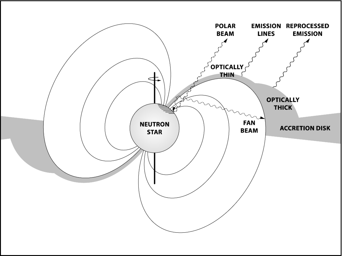
Figure 16: Schematic representation of the proposed structural configuration of X-ray pulsars in the moderately high accretion regime. The (possibly inflated) accretion disk is truncated at approximately the magnetosphere, and a combination of optically thick and thin plasma is trapped at the magnetopsheric boundary. The optically thick material (and the inner disk edge) partially cover the primary emission source and reprocess its emission. At higher latitudes, the material remains optically thin. This is the origin of the emission lines. The source of the primary emission is located at a some height above the NS pole, inside the accretion column. We stress that the drawing is aimed to better illustrate the discussed configuration and does not attempt to realistically reproduce the geometry of an accreting highly magnetized NS. More specifically, for viewing clarity, the emission pattern and direction of the fan and polar beams has been oversimplified and the inner disk radius (and size of the magnetosphere) has been greatly depreciated (e.g., in a more realistic example, both components may illuminate the reprocessing region). The regions where the optically thin and thick plasma are expected to lie have also been presented in a very simplified minimalistic arrangement.

5 Conclusion

We have analyzed the high-quality XMM-Newton observation of SMC X-3 during its recent outburst. The XMM-Newton data where complemented with Swift/XRT observations, which were used to study the long-term behavior of the source. By carrying out a detailed temporal and spectral analysis (including phase-resolved spectroscopy) of the source emission, we found that its behavior and temporal and spectral characteristics fit the theoretical expectations and the previously noted observational traits of accreting highly magnetized NSs at high accretion rates. More specifically, we found indications of a complex emission pattern of the primary pulsed radiation, which most likely involves a combination of a fan-beam emission component directed perpendicularly to the magnetic field axis and a secondary polar-beam component reflected off the NS surface and directed perpendicularly to the primary fan beam (as discussed in, e.g., Basko & Sunyaev 1976; Wang & Frank 1981 and more recently by Trümper et al. 2013).

The spectroscopic analysis of the source further reveals optically thick material located at approximately the boundary of the magnetosphere. The reprocessing region has an angular size (as viewed from the NS) that is large enough to reprocess a considerable fraction of the primary beamed emission, which is remitted in the form of a soft thermal-like component that contributes very little to the pulsed emission. These findings are in agreement with previous works on X-ray pulsars (e.g., Endo et al. 2000; Hickox et al. 2004), but also with the theoretical predictions for highly super-Eddington accretion onto highly magnetized NSs (e.g., King et al. 2017; Mushtukov et al. 2017; Koliopanos et al. 2017), where it has been argued that this reprocessing region grows to the point that it may reprocess the entire pulsar emission.

6 Acknowledgements

The authors thank Maria Petropoulou for valuable advice and stimulating discussion and Olivier Godet for contributing to the RGS analysis. The authors also extend their warm gratitude to Cheryl Woynarski and woyadesign.com for designing the source schematic. Finally we extend our gratitude to the anonymous referee, whose keen observations significantly improved our manuscript.

References

- Antoniou & Zezas (2016) Antoniou, V. & Zezas, A. 2016, MNRAS, 459, 528
- Antoniou et al. (2010) Antoniou, V., Zezas, A., Hatzidimitriou, D., & Kalogera, V. 2010, ApJ, 716, L140
- Arnaud (1996) Arnaud, K. A. 1996, in Astronomical Society of the Pacific Conference Series, Vol. 101, Astronomical Data Analysis Software and Systems V, ed. G. H. Jacoby & J. Barnes, 17
- Bachetti et al. (2014) Bachetti, M., Harrison, F. A., Walton, D. J., et al. 2014, Nature, 514, 202
- Basko (1978) Basko, M. M. 1978, ApJ, 223, 268
- Basko (1980) Basko, M. M. 1980, A&A, 87, 330
- Basko & Sunyaev (1975) Basko, M. M. & Sunyaev, R. A. 1975, A&A, 42, 311
- Basko & Sunyaev (1976) Basko, M. M. & Sunyaev, R. A. 1976, MNRAS, 175, 395
- Becker et al. (2012) Becker, P. A., Klochkov, D., Schönherr, G., et al. 2012, A&A, 544, A123
- Becker & Wolff (2007) Becker, P. A. & Wolff, M. T. 2007, ApJ, 654, 435
- Beloborodov (2002) Beloborodov, A. M. 2002, ApJ, 566, L85
- Blackburn (1995) Blackburn, J. K. 1995, in Astronomical Society of the Pacific Conference Series, Vol. 77, Astronomical Data Analysis Software and Systems IV, ed. R. A. Shaw, H. E. Payne, & J. J. E. Hayes, 367
- Boirin & Parmar (2003) Boirin, L. & Parmar, A. N. 2003, A&A, 407, 1079
- Burderi et al. (2000) Burderi, L., Di Salvo, T., Robba, N. R., La Barbera, A., & Guainazzi, M. 2000, ApJ, 530, 429
- Burnard et al. (1991) Burnard, D. J., Arons, J., & Klein, R. I. 1991, ApJ, 367, 575
- Caballero & Wilms (2012) Caballero, I. & Wilms, J. 2012, Mem. Soc. Astron. Italiana, 83, 230
- Canuto et al. (1971) Canuto, V., Lodenquai, J., & Ruderman, M. 1971, Phys. Rev. D, 3, 2303
- Cash (1979) Cash, W. 1979, ApJ, 228, 939
- Chashkina et al. (2017) Chashkina, A., Abolmasov, P., & Poutanen, J. 2017, ArXiv e-prints
- Christodoulou et al. (2016) Christodoulou, D. M., Laycock, S. G. T., Yang, J., & Fingerman, S. 2016, ApJ, 829, 30
- Clark et al. (1978) Clark, G., Doxsey, R., Li, F., Jernigan, J. G., & van Paradijs, J. 1978, ApJ, 221, L37
- Corbet et al. (2003) Corbet, R. H. D., Edge, W. R. T., Laycock, S., et al. 2003, in Bulletin of the American Astronomical Society, Vol. 35, AAS/High Energy Astrophysics Division #7, 629
- Cowley & Schmidtke (2004) Cowley, A. P. & Schmidtke, P. C. 2004, AJ, 128, 709
- Davies (1990) Davies, S. R. 1990, MNRAS, 244, 93
- De Marco & Ponti (2016) De Marco, B. & Ponti, G. 2016, ApJ, 826, 70
- den Herder et al. (2001) den Herder, J. W., Brinkman, A. C., Kahn, S. M., et al. 2001, A&A, 365, L7
- Díaz Trigo et al. (2014) Díaz Trigo, M., Migliari, S., Miller-Jones, J. C. A., & Guainazzi, M. 2014, A&A, 571, A76
- Díaz Trigo et al. (2006) Díaz Trigo, M., Parmar, A. N., Boirin, L., Méndez, M., & Kaastra, J. S. 2006, A&A, 445, 179
- Dickey & Lockman (1990) Dickey, J. M. & Lockman, F. J. 1990, ARA&A, 28, 215
- Dotan & Shaviv (2011) Dotan, C. & Shaviv, N. J. 2011, MNRAS, 413, 1623
- Edge et al. (2004) Edge, W. R. T., Coe, M. J., Corbet, R. H. D., Markwardt, C. B., & Laycock, S. 2004, The Astronomer’s Telegram, 225
- Endo et al. (2000) Endo, T., Nagase, F., & Mihara, T. 2000, PASJ, 52, 223
- Evans et al. (2007) Evans, P. A., Beardmore, A. P., Page, K. L., et al. 2007, A&A, 469, 379
- Fürst et al. (2016) Fürst, F., Walton, D. J., Harrison, F. A., et al. 2016, ApJ, 831, L14
- Ghosh & Lamb (1979a) Ghosh, P. & Lamb, F. K. 1979a, ApJ, 232, 259
- Ghosh & Lamb (1979b) Ghosh, P. & Lamb, F. K. 1979b, ApJ, 234, 296
- Ghosh & Lamb (1992) Ghosh, P. & Lamb, F. K. 1992, in X-Ray Binaries and the Formation of Binary and Millisecond Radio Pulsars, 487–510
- Ghosh et al. (1977) Ghosh, P., Pethick, C. J., & Lamb, F. K. 1977, ApJ, 217, 578
- Gilfanov (2010) Gilfanov, M. 2010, in Lecture Notes in Physics, Berlin Springer Verlag, Vol. 794, Lecture Notes in Physics, Berlin Springer Verlag, ed. T. Belloni, 17
- Graczyk et al. (2014) Graczyk, D., Pietrzyński, G., Thompson, I. B., et al. 2014, ApJ, 780, 59
- Gregory & Loredo (1996) Gregory, P. C. & Loredo, T. J. 1996, ApJ, 473, 1059
- Hickox et al. (2004) Hickox, R. C., Narayan, R., & Kallman, T. R. 2004, ApJ, 614, 881
- Hickox & Vrtilek (2005) Hickox, R. C. & Vrtilek, S. D. 2005, ApJ, 633, 1064
- Ikhsanov & Mereghetti (2015) Ikhsanov, N. R. & Mereghetti, S. 2015, MNRAS, 454, 3760
- Israel et al. (2017a) Israel, G. L., Belfiore, A., Stella, L., et al. 2017a, Science, 355, 817
- Israel et al. (2017b) Israel, G. L., Papitto, A., Esposito, P., et al. 2017b, MNRAS, 466, L48
- Jahoda et al. (2006) Jahoda, K., Markwardt, C. B., Radeva, Y., et al. 2006, ApJS, 163, 401
- Kaminker et al. (1976) Kaminker, A. D., Fedorenko, V. N., & Tsygan, A. I. 1976, Sov. Ast., 20, 436
- Kennea et al. (2016) Kennea, J. A., Coe, M. J., Evans, P. A., et al. 2016, The Astronomer’s Telegram, 9362
- King & Lasota (2016) King, A. & Lasota, J.-P. 2016, MNRAS, 458, L10
- King et al. (2017) King, A., Lasota, J.-P., & Kluźniak, W. 2017, MNRAS, 468, L59
- Klochkov et al. (2011) Klochkov, D., Staubert, R., Santangelo, A., Rothschild, R. E., & Ferrigno, C. 2011, A&A, 532, A126
- Klus et al. (2014) Klus, H., Ho, W. C. G., Coe, M. J., Corbet, R. H. D., & Townsend, L. J. 2014, MNRAS, 437, 3863
- Kolehmainen et al. (2014) Kolehmainen, M., Done, C., & Díaz Trigo, M. 2014, MNRAS, 437, 316
- Koliopanos & Gilfanov (2016) Koliopanos, F. & Gilfanov, M. 2016, MNRAS, 456, 3535
- Koliopanos et al. (2017) Koliopanos, F., Vasilopoulos, G., Gobet, O., et al. 2017, A&A submitted, 0, 0
- Kosec et al. (2018) Kosec, P., Pinto, C., Fabian, A. C., & Walton, D. J. 2018, MNRAS, 473, 5680
- Krtička et al. (2011) Krtička, J., Owocki, S. P., & Meynet, G. 2011, A&A, 527, A84
- Kuehnel et al. (2015) Kuehnel, M., Kretschmar, P., Nespoli, E., et al. 2015, in Proceedings of “A Synergistic View of the High Energy Sky” - 10th INTEGRAL Workshop (INTEGRAL 2014). 15-19 September 2014. Annapolis, MD, USA. Published online at ¡A href=“http://pos.sissa.it/cgi-bin/reader/conf.cgi?confid=228”¿http://pos.sissa.it/cgi-bin/reader/conf.cgi?confid=228¡/A¿, id.78, 78
- La Barbera et al. (2001) La Barbera, A., Burderi, L., Di Salvo, T., Iaria, R., & Robba, N. R. 2001, ApJ, 553, 375
- La Palombara & Mereghetti (2006) La Palombara, N. & Mereghetti, S. 2006, A&A, 455, 283
- La Palombara et al. (2016) La Palombara, N., Sidoli, L., Pintore, F., et al. 2016, MNRAS, 458, L74
- Larsson (1996) Larsson, S. 1996, A&AS, 117, 197
- Lodenquai et al. (1974) Lodenquai, J., Canuto, V., Ruderman, M., & Tsuruta, S. 1974, ApJ, 190, 141
- Lyubarskii & Syunyaev (1988) Lyubarskii, Y. E. & Syunyaev, R. A. 1988, Soviet Astronomy Letters, 14, 390
- Manousakis et al. (2009) Manousakis, A., Walter, R., Audard, M., & Lanz, T. 2009, A&A, 498, 217
- McBride et al. (2008) McBride, V. A., Coe, M. J., Negueruela, I., Schurch, M. P. E., & McGowan, K. E. 2008, MNRAS, 388, 1198
- Mészáros (1992) Mészáros, P. 1992, High-energy radiation from magnetized neutron stars.
- Meszaros & Nagel (1985) Meszaros, P. & Nagel, W. 1985, ApJ, 299, 138
- Mushtukov et al. (2017) Mushtukov, A. A., Suleimanov, V. F., Tsygankov, S. S., & Ingram, A. 2017, MNRAS, 467, 1202
- Mushtukov et al. (2015) Mushtukov, A. A., Suleimanov, V. F., Tsygankov, S. S., & Poutanen, J. 2015, MNRAS, 454, 2539
- Nagel (1981) Nagel, W. 1981, ApJ, 251, 288
- Negoro et al. (2016) Negoro, H., Nakajima, M., Kawai, N., et al. 2016, The Astronomer’s Telegram, 9348
- Ng et al. (2010) Ng, C., Díaz Trigo, M., Cadolle Bel, M., & Migliari, S. 2010, A&A, 522, A96
- Okazaki et al. (2013) Okazaki, A. T., Hayasaki, K., & Moritani, Y. 2013, PASJ, 65, 41
- Paul et al. (1996) Paul, B., Agrawal, P. C., Rao, A. R., & Manchanda, R. K. 1996, Bulletin of the Astronomical Society of India, 24, 729
- Paul et al. (1997) Paul, B., Agrawal, P. C., Rao, A. R., & Manchanda, R. K. 1997, A&A, 319, 507
- Pietrzyński et al. (2013) Pietrzyński, G., Graczyk, D., Gieren, W., et al. 2013, Nature, 495, 76
- Pinto et al. (2017a) Pinto, C., Alston, W., Soria, R., et al. 2017a, MNRAS, 468, 2865
- Pinto et al. (2017b) Pinto, C., Fabian, A., Middleton, M., & Walton, D. 2017b, Astronomische Nachrichten, 338, 234
- Pinto et al. (2016) Pinto, C., Middleton, M. J., & Fabian, A. C. 2016, Nature, 533, 64
- Pintore et al. (2017) Pintore, F., Zampieri, L., Stella, L., et al. 2017, ApJ, 836, 113
- Postnov et al. (2015) Postnov, K. A., Gornostaev, M. I., Klochkov, D., et al. 2015, MNRAS, 452, 1601
- Pottschmidt et al. (2016) Pottschmidt, K., Ballhausen, R., Wilms, J., et al. 2016, The Astronomer’s Telegram, 9404
- Poutanen et al. (2007) Poutanen, J., Lipunova, G., Fabrika, S., Butkevich, A. G., & Abolmasov, P. 2007, MNRAS, 377, 1187
- Poutanen et al. (2013) Poutanen, J., Mushtukov, A. A., Suleimanov, V. F., et al. 2013, ApJ, 777, 115
- Ramsay et al. (2002) Ramsay, G., Zane, S., Jimenez-Garate, M. A., den Herder, J.-W., & Hailey, C. J. 2002, MNRAS, 337, 1185
- Rea et al. (2004) Rea, N., Israel, G. L., Di Salvo, T., Burderi, L., & Cocozza, G. 2004, A&A, 421, 235
- Reig (2011) Reig, P. 2011, Ap&SS, 332, 1
- Reig & Nespoli (2013) Reig, P. & Nespoli, E. 2013, A&A, 551, A1
- Reig et al. (2012) Reig, P., Torrejón, J. M., & Blay, P. 2012, MNRAS, 425, 595
- Romanova et al. (2004) Romanova, M. M., Ustyugova, G. V., Koldoba, A. V., & Lovelace, R. V. E. 2004, ApJ, 610, 920
- Schönherr et al. (2007) Schönherr, G., Wilms, J., Kretschmar, P., et al. 2007, A&A, 472, 353
- Schulz et al. (2002) Schulz, N. S., Canizares, C. R., Lee, J. C., & Sako, M. 2002, ApJ, 564, L21
- Shakura & Sunyaev (1973) Shakura, N. I. & Sunyaev, R. A. 1973, A&A, 24, 337
- Shimura & Takahara (1995) Shimura, T. & Takahara, F. 1995, ApJ, 445, 780
- Sibgatullin & Sunyaev (2000) Sibgatullin, N. R. & Sunyaev, R. A. 2000, Astronomy Letters, 26, 699
- Staubert et al. (2007) Staubert, R., Shakura, N. I., Postnov, K., et al. 2007, A&A, 465, L25
- Sturm et al. (2013) Sturm, R., Haberl, F., Pietsch, W., et al. 2013, A&A, 558, A3
- Suleimanov et al. (2007) Suleimanov, V. F., Lipunova, G. V., & Shakura, N. I. 2007, Astronomy Reports, 51, 549
- Sunyaev & Titarchuk (1980) Sunyaev, R. A. & Titarchuk, L. G. 1980, A&A, 86, 121
- Townsend et al. (2017) Townsend, L. J., Kennea, J. A., Coe, M. J., et al. 2017, arXiv:1701.02336
- Trümper et al. (2013) Trümper, J. E., Dennerl, K., Kylafis, N. D., Ertan, Ü., & Zezas, A. 2013, ApJ, 764, 49
- Tsygankov et al. (2017) Tsygankov, S. S., Doroshenko, V., Lutovinov, A. A., Mushtukov, A. A., & Poutanen, J. 2017, arXiv:1702.00966
- Tsygankov et al. (2007) Tsygankov, S. S., Lutovinov, A. A., Churazov, E. M., & Sunyaev, R. A. 2007, Astronomy Letters, 33, 368
- Tsygankov et al. (2010) Tsygankov, S. S., Lutovinov, A. A., & Serber, A. V. 2010, MNRAS, 401, 1628
- Udalski et al. (2015) Udalski, A., Szymański, M. K., & Szymański, G. 2015, Acta Astron., 65, 1
- Vasco et al. (2011) Vasco, D., Klochkov, D., & Staubert, R. 2011, A&A, 532, A99
- Vasilopoulos et al. (2016) Vasilopoulos, G., Haberl, F., Delvaux, C., Sturm, R., & Udalski, A. 2016, MNRAS, 461, 1875
- Vasilopoulos et al. (2017) Vasilopoulos, G., Haberl, F., & Maggi, P. 2017, MNRAS accepted, 0, 0
- Vasilopoulos et al. (2014) Vasilopoulos, G., Haberl, F., Sturm, R., Maggi, P., & Udalski, A. 2014, A&A, 567, A129
- Vasilopoulos et al. (2013) Vasilopoulos, G., Maggi, P., Haberl, F., et al. 2013, A&A, 558, A74
- Vasilopoulos & Petropoulou (2016) Vasilopoulos, G. & Petropoulou, M. 2016, MNRAS, 455, 4426
- Verner et al. (1996) Verner, D. A., Ferland, G. J., Korista, K. T., & Yakovlev, D. G. 1996, ApJ, 465, 487
- Walter & Ferrigno (2016) Walter, R. & Ferrigno, C. 2016, arXiv:1608.06530
- Walter et al. (2015) Walter, R., Lutovinov, A. A., Bozzo, E., & Tsygankov, S. S. 2015, A&A Rev., 23, 2
- Wang & Frank (1981) Wang, Y.-M. & Frank, J. 1981, A&A, 93, 255
- Watson et al. (2009) Watson, M. G., Schröder, A. C., Fyfe, D., et al. 2009, A&A, 493, 339
- Weng et al. (2017) Weng, S.-S., Ge, M.-Y., Zhao, H.-H., et al. 2017, ApJ, 843, 69
- White et al. (1983) White, N. E., Swank, J. H., & Holt, S. S. 1983, ApJ, 270, 711
- Wilms et al. (2011) Wilms, Juett, Schulz, & Nowak. 2011, ApJ
- Wilms et al. (2000) Wilms, J., Allen, A., & McCray, R. 2000, ApJ, 542, 914
- Wilson et al. (2008) Wilson, C. A., Finger, M. H., & Camero-Arranz, A. 2008, ApJ, 678, 1263