3D Face Reconstruction with Region Based Best Fit Blending Using Mobile Phone for Virtual Reality Based Social Media

1 Introduction

Reconstruction 3D face models has been a challenging task for the last two decades, because even a small amount of changes can have a huge effect on the recognizability and accuracy of the generated model. Therefore, perfectly modelling a 3D human face still remains one of the quintessential problems of computer vision. Also with the rapid increase of applications of virtual reality (VR) in gaming as well use use of VR application for making VR based social media, the task of making real-time 3D model of head which can be later mounted on avatar bodies have become very important [1, 2, 3, 4, 5, 6, 7]. So far the easiest, fastest and most accurate methods have benefited from depth information that can be captured with recording devices like RGB-D cameras [8, 9, 10, 11, 12, 13, 14] or 3D scanners [15, 16, 17, 18]. However, nowadays development has been directed towards mobile devices, which limited to only using RGB information.

As an alternative commodity mobile phones that have their own on-device stereo cameras [19, 20, 21, 22] can be used to recreate the depth data. Models created with passive multi-view stereo [23, 24] have distinct features but very rough surfaces. Due to the noisiness of the input data heavy smoothing needs to be applied, resulting models that don’t have finer details around more complex features like the eyes and nostrils.

For 3D face reconstruction based on regular input images or videos, a large variety of methods and algorithms have been developed. The most conventional approach has been to use a 3D morphable head model [25, 26]. Even though each researcher has used different metrics and methods, the main idea has been to minimize the error between input image and the 2D render of the model. The models features are iteratively morphed to minimize the difference between the input image and the image with the render of the model, using suitable lighting and orientation, overlaid on the original face. A huge downside to these methods is that they require a lot of processing power and time. [25, 27]. Another popular method is silhouette extraction, where the outer silhouette of a face is detected in video frames and the base model(without texture) is then constructed iteratively [28, 29]. In [30] and [31] landmark based shape reconstruction of 3D faces, which is very similar to RGB-D reconstruction, is used. In these cases features extracted using SIFT, SURF etc. were utilized. In some cases, the missing depth info was approximated using shading and lighting source estimation [32]. All of the above mentioned methods suffer from high complexity, which can result in longer computational time.

More efficient methods for face reconstruction generally rely on the detection of facial feature points or sparse landmarks and then stretching of a generic base model to produce a realistic output [33, 34, 35, 36]. Among those are some that have even been specifically designed for mobile applications, but unfortunately the produced models tend to lack distinct features and the end result looks generic [37]. Even though recognizable result can be achieved using excellent texturing techniques, the base model itself looks nothing like the real person. The algorithm behind Landmark-based Model-free 3D Face Shape Reconstruction [38] tries to address the problem of generic looking outputs by avoiding statistical models as the base structure. They managed to produce genuine-looking models, but as the output is untextured and not a simple quadrilateral mesh structure, it is unusable for consumer applications.

In this paper we present a computationally light method for creating a 3D face model from video or image input, by constructing models for 4 key regions and later blending them. The method benefits from a high quality 3D scanned model database consisting of 200+ male head. As a pre-processing step all 4 key areas are individually rendered for each entry. As a first step of the method, the detected face is separated from the frame and 68 feature points are extracted. The face is divided into the 4 key regions, which are matched up against corresponding rendered areas of the database. These comparisons yield weights that are then used to combine a model from the predefined face regions. A stretching method similar to the ones described in [33, 34, 35, 36] is the applied. The model is then further morphed using the 68 feature points and their corresponding vertexes on the model in order to restore facial proportions.

A texture is created by aligning the input images using piece-wise affine transformations to fit the UV map of the model. As an output our proposed method creates a 3D model with accurate facial features and fixed vertexes. This enables rigging, simple integration into existing systems or reintegration into the database while using minimal computational power. As a prerequisite, our method places some constraints on the input images and video, namely full visibility of the face with minimal facial hair and somewhat fixed lighting conditions.

2 Proposed method

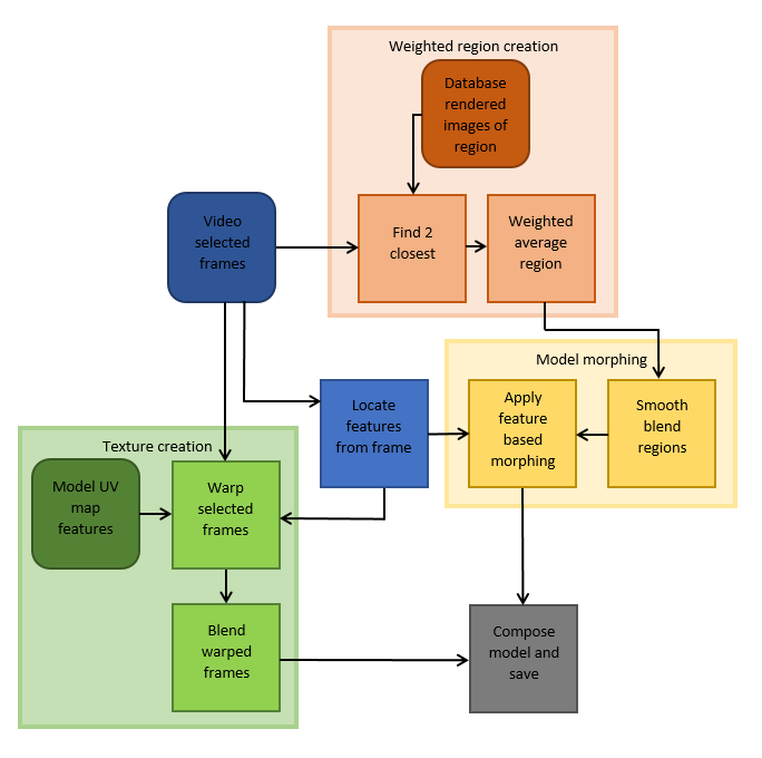
In this section a novel methodology for making 3D models from videos or image sequences is proposed. This approach benefits from a unique reference database of 3D head scans. As illustrated in Fig. 1, the process can be divided into four main parts:

• feature extraction

• selection closest models

• model creation

• texture creation.

Fig. 1: Block diagram describing the overall process

2.1 Database

2.1.1 Data description

The preliminary database consisted of textured 3D scans of 217 mostly Caucasian male head area, that were morphed and simplified so all shared the same vertex mapping and count. All of the textures were also warped to fit the same UV map. In this step everything behind the head from the original scans was discarded, including the hair and the ears. In the original data some of the scans contained facial hair or severe noise/deformations. However the rest of the regions were usually not affected.

The pre-processed model consists of a mesh that contains 6000 quadrilateral faces and a corresponding 2048x2048 RGB texture. The indexes of the vertexes in all of the models are ordered and don’t vary from model to model.

2.1.2 Rendering regions

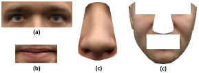
An auxiliary database of rendered face regions was made in order to find the weights of each model based on the input image. All of the models were rendered in frontal orientation using perspective cameras with 5 directional light sources from the front, sides and top - all aimed towards the center of the head. The rendered images were then cut into 4 sections which correspond to the eyes, nose, mouth regions and rest of the face as shown in Fig. 2.

Fig. 2: Cut out sections of a rendered model from the model database. The 4 sections represent the eyes (a), mouth (b), nose (c) and the rest of the face (d) regions.

2.2 Feature extraction

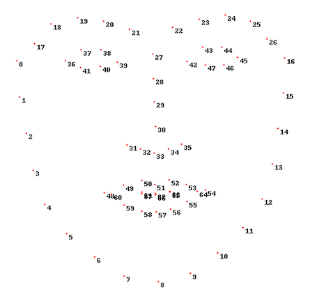
For the facial feature extraction we use facial analysis toolkit [39] to estimate and extract $68$ facial feature points from the input video sequence. Due to limitations of the toolkit, the input face must have a near neutral face, with no eye-wear or thick facial hair which obstruct the feature detection. These points are illustrated in 3. The algorithm also outputs the rotation parameters, so this can be used to pick the frontally best aligned frame as the main reference for creating the model. This also allows alignment of the face to a frontal one in case of slight tilt or rotation.

As the next step the area containing feature points is extracted and the feature points from that area are normalized to fit between $0$ and $1$.

Fig. 3: The 68 feature points that are extracted

2.3 Region-based selection and weight calculation

In this step we calculate similarities between database regions and the input grayscale regions. There are altogether three different similarity indexes used: PCA based measure, SSIM [40] (structural similarity index) and a LBP(local binary pattern) histograms difference measure [41].

In the PCA based approach the database images are first vectorized and the covariance matrix of these vectors is found. The principal components and score vectors are stored for future use. When looking for the closest match the corresponding image region is also vectorized and its score vector on the principal components is found. We treat the Eucleidean difference between the score vectors as the error and its’ inverse as the similarity measure.

Since the SSIM finds the similarity between two images, the maximum being one, we use the dissimilarity ($1-ssuim$) as the error. In case of LBP features we also apply PCA to the output feature and find the distances as described earlier.

For picking the closest mouth and nose regions, SSIM was used. For eyes we used LBP as they have the most high frequency data and for face shape we used PCA based approach as the placement zero and non-zero values has high impact on this measure.

For each region a similarity function between database rendered regions and the regions extracted from the frontal face is applied. After which the corresponding similarity function, an error vector is obtained for each region. Let us denote it by $E=(E_{1},E_{2},\ldots,E_{n})$, where $n$ is the number of reference heads in the database. Let $I$ denote the set of indexes of the database models corresponding to smallest error. The weights $W_{i},i\in I$ are calculated according to the formula:

$$W_{i}=\frac{E_{i}^{-1}}{\sum_{j\in I}{E_{j}^{-1}}}$$ (1)

The rest of the weights are set to zero: $W_{i}=0$, $\forall i\not\in I$

Based on the errors of the similarity three (or in some cases 1) closest matches are picked for each region, and weights that are inversely proportional to the errors are assigned. The weights are normalized to they sum to 1.

2.4 Blended model creation

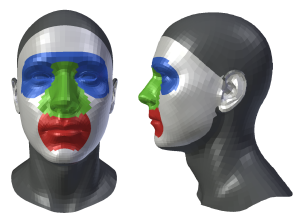
The model is separated into 5 primary regions as shown in Fig. 4, out of these regions, only the eyes, nose, mouth regions and rest of the face area are used. For each region 3D models $AM$ are created as blendshapes [28] from weighted combinations of an array of models $M=(M_{0},M_{1},M_{2},\dots,M_{n})$ and their corresponding weights $W=(W_{0},W_{1},W_{2},\dots,W_{n})$, as in formula 2. Each model ($AM$) has its corresponding region of interest signified with an array of indexes called $I_{A}$.

Out of the four models created, the one representing the rest of the face will be called the base model $BM$. The $BM$ will be the starting model, on which the other weighted models are added one-by-one. The base model $BM$ also has its own corresponding index array called $I_{B}$.

$$BM=M_{i}\cdot W_{i}^{T}$$ (2)

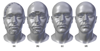
Then regions from these composite 3D models are combined together to form the overall base shape of the 3D model as shown in Fig. 5a.

To minimize the effect of large transitions between regions, mean locations are calculated for the overlapping vertexes of 2 combined regions. The vertex indexes for this new region will be denoted as $I_{AB}=I_{A}\cap I_{B}$.

The vector originating from the mean point of the added region to the mean of the existing region is found using formula 3.

$$\vec{s}_{BA}=\frac{1}{|I_{AB}|}\cdot\sum_{i\in I_{AB}}(v_{i}^{B}-v_{i}^{A})$$ (3)

To reduce the large effect of small locational variations that have later a big effect on the smoothing process, the vector $\frac{1}{2}s_{BA}$ is added to the points in the added region using the formula 4.

$$v_{i}^{A}=v_{i}^{A}+\frac{\vec{s}_{BA}}{2}\quad i\in I$$ (4)

To further smooth the transition between different regions, a blending function is applied when calculating the model weights for each vertex. This can be seen as the transition from model (b) to (c) in Fig. 5. In order to scale the blending function for the added regions area, the maximum translations along the $X$ and $Y$ axes of the added region are calculated.

$$\Delta_{x}=\max_{i\in I_{A}}\{x_{i}^{A}\}-\min_{i\in I_{A}}\{x_{i}^{A}\}$$ (5)

Where $x_{i}^{A}$ is the $X$ axis component of $v_{i}^{A}$. $\Delta_{y}$ is found using a similar function as 5 and they will be denoted as $\Delta=(\Delta_{x},\Delta_{y})$.

The distances of all of the added region points from the their mean can then be calculated and normalized using the function 6.From now on $j$ will denote the index of a vertex from the model.

$$\delta_{j}=||\frac{\mu_{AM_{I_{A}}}-v_{i}^{A}}{\Delta}||\quad i\in I$$ (6)

As all of the distances will be in reference to the mean of the added region, similar calculations will not be applied to the base region.

A transition weight function $\mathit{twf}(x)$ is then applied to each of the point distances to get the weights for each vertex. The two regions are then combined using:

$$\mathit{twf}(\delta_{j})=1.013-\frac{1.019}{1+(\frac{\delta_{i}}{0.264})^{3.244}}$$ (7)

$$BM_{j}=BM_{j}\cdot(1-\mathit{twf}(\delta_{j}))+AM_{j}\cdot\mathit{twf}(\delta_{j})$$ (8)

Since the nose region has some overlapping areas with the eye and the mouth region, it is added to the base model first. Next the eye and mouth regions are added, though here the order plays no role as they don’t share any vertexes.

Fig. 4: The 5 primary regions as shown in colors are used for linear weighted combinations to generate the base model. The eye region is shown in blue, the nose region is shown in green, the mouth region is shown in red, the rest of the face region is shown in white and the unused parts of the model are shown in gray.

Fig. 5: Processing steps for blending and morphing the 3D model regions to create an output model. The weighted model regions are combined to form the base shape of the output model (a). To ease the transitions between different regions the regions are first aligned with one another (b) and then the overlapping areas are blended together using a blending function (c). The final combined model is then further morphed (d) to fit the input image

2.5 Model morphing

The generated blended model $BM$ has features which resemble the desired face, but some of the proportions are off. Due to that the model is further morphed so key features match their actual locations. The model has 68 vertexes mapped to 68 feature points $F=\{F_{i}\}\quad i\in\{1,2,\dots,68\}$ where value of $i$ will remain the same for all of the following functions. For each mapped vertex a movement vector to the feature location is calculated as:

$$\vec{f}_{i}=F_{i}-BM_{i}$$ (9)

For each of the points in the model, a distance is calculated from each mapped vertex and a adjustment weight function $\mathit{awf}(x)$ is applied to get the weight of each vector for each vertex.

$$d_{ji}=|F_{i}-BM_{j}|$$ (10)

$$\mathit{awf}(d_{ji})=1-\bigg{(}{1+e^{\big{(}\frac{-d_{ji}}{\sigma_{i}^{2}\cdot k}+0.5\big{)}\cdot 7}}\bigg{)}^{-1}$$ (11)

Where $\sigma_{i}$ defines the drop-off rate for the adjustment weight function, which is separately defined for each feature point, $k$ is a similar multiplier but it is independent from the feature point values. The vectors $\vec{f}_{i}$ are then multiplied by the weights for each point and summed together:

$$\vec{s}_{j}=\sum_{i=1}^{n}(\mathit{awf}(d_{ji})\cdot\vec{f}_{i})$$ (12)

Then the sum of these weights $r_{j}$ is calculated by:

$$r_{j}=\sum_{i=1}^{n}\mathit{awf}(d_{ji})$$ (13)

The resulting vector $s_{j}$ is further divided by the sum of the weights, if $r_{j}>1$. This is done to keep densely packed features from overwhelming vertexes with their respective changes. The final vectors are added to every point in the model.

$$BM_{j}=\begin{cases}BM_{j}+\vec{s}_{j},&\quad\mathrm{if}\quad r_{j}\leq 1\\ BM_{j}+\frac{\vec{s}_{j}}{r_{j}},&\quad\mathrm{if}\quad r_{j}>1\end{cases}$$ (14)

Since some feature vertexes define larger areas like the eyebrows and chin, while others define finer details like the eyes and nostrils, the features also have their own weights called $\sigma_{i}$. These weights allow for different features to have different adjustment weight functions as shown in the formula 11. The morphing is applied 3 times with 3 different $k$ values, starting with more general features and ending with smaller details, where the adjustment weight function sets the weights of points that have larger $\sigma_{i}$ values to zero.

2.6 Texture creation

The texture of any 3D model is strongly bound by the UV map. By hand it is difficult to morph images into a form that would correspond to this map. In this work an average texture was first created based on the database textures Fig. 7a. Since all of the models in the database have a corresponding UV map, the input image had to be transformed to fit the same map. In order to warp the input image appropriately, $68$ vertexes on the UV map were marked corresponding to the $68$ feature points on the input image.

For texture creation we assume that there are no distinctive shadows present in the video sequence. Based on the extracted feature points and rotations, three frames are picked from the sequence based on yaw at approximately $30$ degrees on both sides and the frontal frame, as in figure6. From the face area also the median face color was extracted.

Fig. 6: An example of images picked to combine

Fig. 7: The average texture created from the existing textures in the database on the left and the input image fitted to the UV map on the left

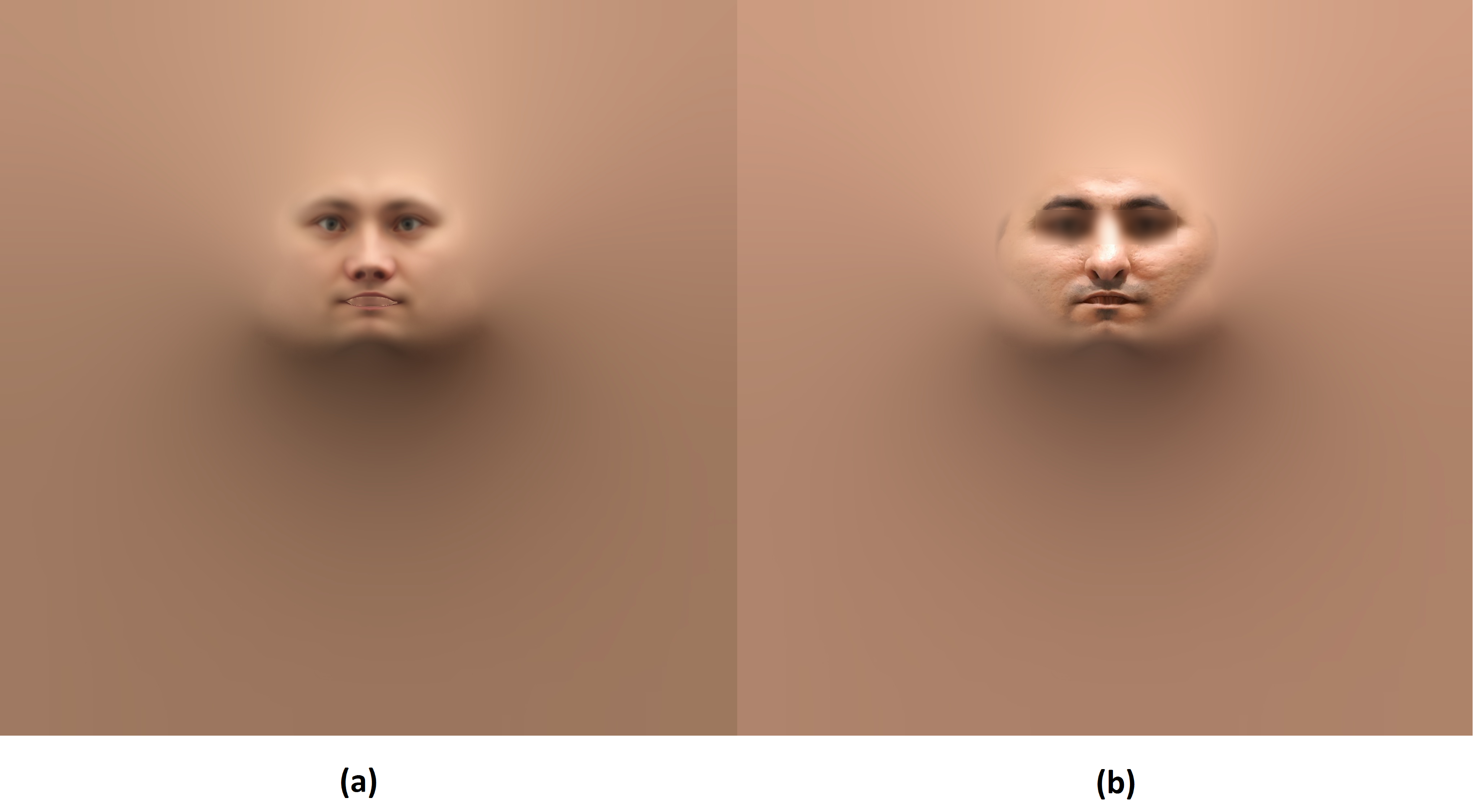
As the next step the average texture colors are shifted to match the median skin tone to assure a smooth and natural transition on the edges of the skin. Then the frames are piece-wise affinely transformed into an image of size $2048\times 2048$ and blended together into a partial texture. This however has very sharp edges and lots of black pixels, so it is then blended only on the edges with the underlying and already shifted average texture. The average texture and the resulting texture can be seen in Fig. 7b.

3 Experimental results

We evaluated our method with several faces, some of which were included in the original scanned database. This was done in order to test the method’s model selection and reconstruction proficiency.

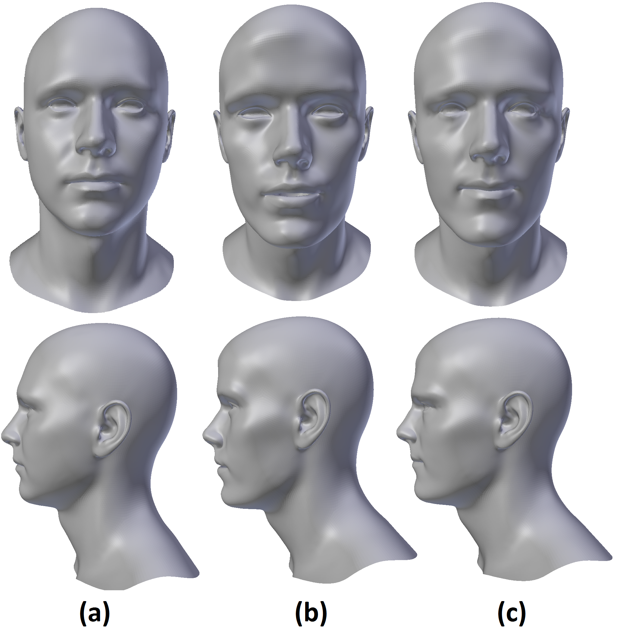
For the faces of people included in the 3D scanned database, the system selected most of the facial features that matched the person. In some cases a different mouth or a set of eyes were chosen when the scanned emotion and the emotion in the captured image were different. This is illustrated by Fig. 8, where the participant had a more surprised facial expressions during the scan and a neutral face during the recording. Regardless, the resulting models were nearly identical to the original scanned versions of those faces.

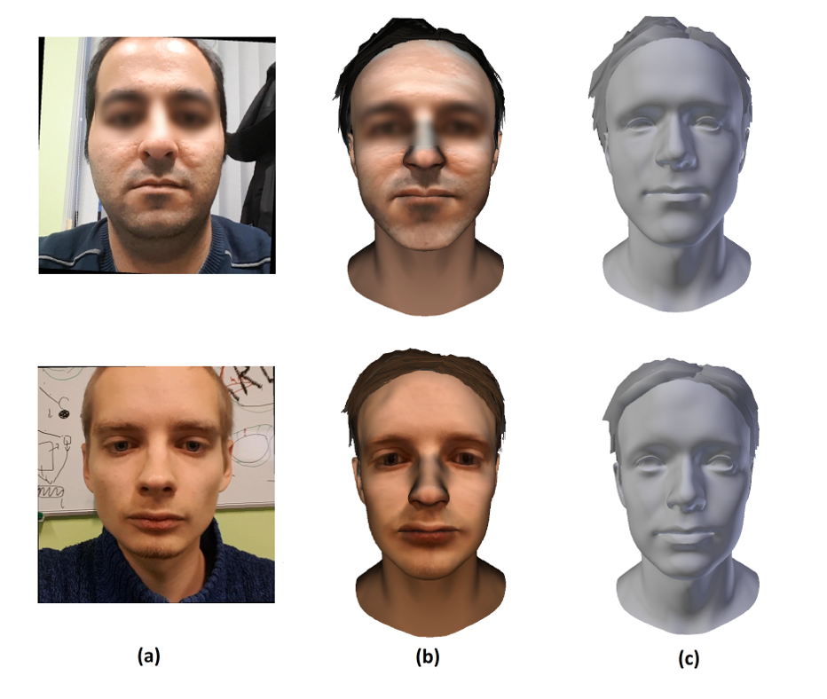
In case of subjects that were not in the database, the system managed to choose facial features that were remarkably similar to the desired face. On occasions where no corresponding feature existed in the database, a blended version from 2 nearest features was created. The result of this blending were not always very similar to the original. This shortcoming can be seen Fig. 9, for the nose in the first row had no structurally similar nose in the entire database.

The goodness of the method was largely limited by the feature detection and the nature of the database. The database contained very little information on the general shape of the head and the feature detection method was very unreliable when it came to detecting the shape of larger areas like the chin. Because of that the resulting heads tended to have the same overall structure. This is very visible in case of the model in the first row in Fig. 9 that has a jawline which is smaller and sharper jawline than expected.

The recordings were conducted with a Samsung Galaxy S7 and the model creation process was run on an i7-4790@3.6GHz CPU with MATLAB 2015a. The whole process, including the recording of a 10 second clip, took about 3 minutes per model. For an i7@4.2GHZ with MATLAB 2016b the model generation took less than a minute.

Fig. 8: An average model from the scanned database (a), a scanned model (b) and the reconstructed version using a mobile phones camera (c).

Fig. 9: Textured (b) and untextured (c) models generated from the example input images (a) using the developed method. Both models have a manually created hair mesh. Neither participants had scanned counterparts in the model database.

4 Conclusion

In this paper, a method of recreating 3D facial models from portrait data, which uses very little computational power in order to produce a recognizable facial model, was proposed. The main idea behind our system is finding the closest matching models for different facial regions and then combining them into a single coherent model. We have also presented a novel and simple method of texturing the resulting model by piece-wise affinely transforming input images to fit a desired UV map based on detected feature points.

Our experimental evaluation has shown that our method is able to select the best corresponding facial features within a reasonable time frame. Our method has also partly overcome the problem of average looking models, which is a huge obstacle in methods that only use stretching to recreate shape. Unfortunately our method is still susceptible to problems relating to the overall shape of the head. This can be fixed with better facial feature extraction methods and with a database that includes a good selection of head shapes. The method can easily be made more robust by rendering the regions with more refined parameters.

References

- [1] J. L. Olson, D. M. Krum, E. A. Suma, and M. Bolas, “A design for a smartphone-based head mounted display,” in Virtual Reality Conference (VR), 2011 IEEE. IEEE, 2011, pp. 233–234.
- [2] B. S. Santos, P. Dias, A. Pimentel, J.-W. Baggerman, C. Ferreira, S. Silva, and J. Madeira, “Head-mounted display versus desktop for 3d navigation in virtual reality: a user study,” Multimedia Tools and Applications, vol. 41, no. 1, p. 161, 2009.
- [3] J.-S. Kim and S.-M. Choi, “A virtual environment for 3d facial makeup,” Virtual Reality, pp. 488–496, 2007.
- [4] G. Anbarjafari, “An objective no-reference measure of illumination assessment,” Measurement Science Review, vol. 15, no. 6, pp. 319–322, 2015.
- [5] B. J. Fernández-Palacios, D. Morabito, and F. Remondino, “Access to complex reality-based 3d models using virtual reality solutions,” Journal of Cultural Heritage, vol. 23, pp. 40–48, 2017.
- [6] D. Zeng, H. Chen, R. Lusch, and S.-H. Li, “Social media analytics and intelligence,” IEEE Intelligent Systems, vol. 25, no. 6, pp. 13–16, 2010.
- [7] D. Trenholme and S. P. Smith, “Computer game engines for developing first-person virtual environments,” Virtual reality, vol. 12, no. 3, pp. 181–187, 2008.
- [8] E. Avots, M. Daneshmand, A. Traumann, S. Escalera, and G. Anbarjafari, “Automatic garment retexturing based on infrared information,” Computers & Graphics, vol. 59, pp. 28–38, 2016.
- [9] T. Yamasaki, I. Nakamura, and K. Aizawa, “Fast face model reconstruction and synthesis using an rgb-d camera and its subjective evaluation,” in Multimedia (ISM), 2015 IEEE International Symposium on. IEEE, 2015, pp. 53–56.
- [10] S. Ding, Y. Li, S. Cao, Y. F. Zheng, and R. L. Ewing, “From rgbd image to hologram,” in Aerospace and Electronics Conference (NAECON) and Ohio Innovation Summit (OIS), 2016 IEEE National. IEEE, 2016, pp. 387–390.
- [11] X. Huang, J. Cheng, and X. Ji, “Human contour extraction from rgbd camera for action recognition,” in Information and Automation (ICIA), 2016 IEEE International Conference on. IEEE, 2016, pp. 1822–1827.
- [12] L. Valgma, M. Daneshmand, and G. Anbarjafari, “Iterative closest point based 3d object reconstruction using rgb-d acquisition devices,” in Signal Processing and Communication Application Conference (SIU), 2016 24th. IEEE, 2016, pp. 457–460.
- [13] C. Ding and L. Liu, “A survey of sketch based modeling systems,” Frontiers of Computer Science, vol. 10, no. 6, pp. 985–999, 2016.
- [14] I. Lüsi and G. Anbarjafari, “Mimicking speaker’s lip movement on a 3d head model using cosine function fitting,” Bulletin of the Polish Academy of Sciences Technical Sciences, vol. 65, no. 5, pp. 733–739, 2017.
- [15] V. Blanz, K. Scherbaum, and H.-P. Seidel, “Fitting a morphable model to 3d scans of faces,” in Computer Vision, 2007. ICCV 2007. IEEE 11th International Conference on. IEEE, 2007, pp. 1–8.
- [16] A. Traumann, M. Daneshmand, S. Escalera, and G. Anbarjafari, “Accurate 3d measurement using optical depth information,” Electronics Letters, vol. 51, no. 18, pp. 1420–1422, 2015.
- [17] M. Daneshmand, A. Aabloo, C. Ozcinar, and G. Anbarjafari, “Real-time, automatic shape-changing robot adjustment and gender classification,” Signal, Image and Video Processing, vol. 10, no. 4, pp. 753–760, 2016.
- [18] I. Fateeva, M. A. Rodriguez, S. R. Royo, and C. Stiller, “Applying 3d least squares matching technique for registration of data taken with an 3d scanner of human body,” in Sensors and Measuring Systems 2014; 17. ITG/GMA Symposium; Proceedings of. VDE, 2014, pp. 1–5.
- [19] K. Kolev, P. Tanskanen, P. Speciale, and M. Pollefeys, “Turning mobile phones into 3d scanners,” in Proceedings of the IEEE Conference on Computer Vision and Pattern Recognition, 2014, pp. 3946–3953.
- [20] P. Ondrúška, P. Kohli, and S. Izadi, “Mobilefusion: Real-time volumetric surface reconstruction and dense tracking on mobile phones,” IEEE transactions on visualization and computer graphics, vol. 21, no. 11, pp. 1251–1258, 2015.
- [21] P. Tanskanen, K. Kolev, L. Meier, F. Camposeco, O. Saurer, and M. Pollefeys, “Live metric 3d reconstruction on mobile phones,” in Proceedings of the IEEE International Conference on Computer Vision, 2013, pp. 65–72.
- [22] H. Zhu, Y. Nie, T. Yue, and X. Cao, “The role of prior in image based 3d modeling: a survey,” Frontiers of Computer Science, vol. 11, no. 2, pp. 175–191, 2017.
- [23] F. Maninchedda, C. Häne, M. R. Oswald, and M. Pollefeys, “Face reconstruction on mobile devices using a height map shape model and fast regularization,” in 3D Vision (3DV), 2016 Fourth International Conference on. IEEE, 2016, pp. 489–498.
- [24] H. Jain, O. Hellwich, and R. Anand, “Improving 3d face geometry by adapting reconstruction from stereo image pair to generic morphable model,” in Information Fusion (FUSION), 2016 19th International Conference on. IEEE, 2016, pp. 1720–1727.
- [25] V. Blanz and T. Vetter, “A morphable model for the synthesis of 3d faces,” in Proceedings of the 26th annual conference on Computer graphics and interactive techniques. ACM Press/Addison-Wesley Publishing Co., 1999, pp. 187–194.
- [26] E. Wood, T. Baltrušaitis, L.-P. Morency, P. Robinson, and A. Bulling, “A 3d morphable eye region model for gaze estimation,” in European Conference on Computer Vision. Springer, 2016, pp. 297–313.
- [27] V. Blanz and T. Vetter, “Face recognition based on fitting a 3d morphable model,” IEEE Transactions on pattern analysis and machine intelligence, vol. 25, no. 9, pp. 1063–1074, 2003.
- [28] J. P. Lewis, K. Anjyo, T. Rhee, M. Zhang, F. H. Pighin, and Z. Deng, “Practice and theory of blendshape facial models.” Eurographics (State of the Art Reports), vol. 1, no. 8, 2014.
- [29] C. Baumberger, M. Reyes, M. Constantinescu, R. Olariu, E. de Aguiar, and T. O. Santos, “3d face reconstruction from video using 3d morphable model and silhouette,” in Graphics, Patterns and Images (SIBGRAPI), 2014 27th SIBGRAPI Conference on. IEEE, 2014, pp. 1–8.
- [30] P. Dou, Y. Wu, S. K. Shah, and I. A. Kakadiaris, “Robust 3d face shape reconstruction from single images via two-fold coupled structure learning,” in Proc. British Machine Vision Conference, 2014, pp. 1–13.
- [31] J. Choi, G. Medioni, Y. Lin, L. Silva, O. Regina, M. Pamplona, and T. C. Faltemier, “3d face reconstruction using a single or multiple views,” in Pattern Recognition (ICPR), 2010 20th International Conference on. IEEE, 2010, pp. 3959–3962.
- [32] I. Kemelmacher-Shlizerman and R. Basri, “3d face reconstruction from a single image using a single reference face shape,” IEEE transactions on pattern analysis and machine intelligence, vol. 33, no. 2, pp. 394–405, 2011.
- [33] Q. Zhang and L. Shi, “3d face model reconstruction based on stretching algorithm,” in Cloud Computing and Intelligent Systems (CCIS), 2012 IEEE 2nd International Conference on, vol. 1. IEEE, 2012, pp. 197–200.
- [34] W. Lin, H. Weijun, C. Rui, and W. Xiaoxi, “Three-dimensional reconstruction of face model based on single photo,” in Computer Application and System Modeling (ICCASM), 2010 International Conference on, vol. 3. IEEE, 2010, pp. V3–674.
- [35] X. Fan, Q. Peng, and M. Zhong, “3d face reconstruction from single 2d image based on robust facial feature points extraction and generic wire frame model,” in Communications and Mobile Computing (CMC), 2010 International Conference on, vol. 3. IEEE, 2010, pp. 396–400.
- [36] T. Wu, F. Zhou, and Q. Liao, “A fast 3d face reconstruction method from a single image using adjustable model,” in Acoustics, Speech and Signal Processing (ICASSP), 2016 IEEE International Conference on. IEEE, 2016, pp. 1656–1660.
- [37] C. Qu, E. Monari, T. Schuchert, and J. Beyerer, “Fast, robust and automatic 3d face model reconstruction from videos,” in Advanced Video and Signal Based Surveillance (AVSS), 2014 11th IEEE International Conference on. IEEE, 2014, pp. 113–118.
- [38] C. van Dam, R. Veldhuis, and L. Spreeuwers, “Landmark-based model-free 3d face shape reconstruction from video sequences,” in Biometrics Special Interest Group (BIOSIG), 2013 International Conference of the. IEEE, 2013, pp. 1–5.
- [39] T. Baltrušaitis, P. Robinson, and L.-P. Morency, “Openface: an open source facial behavior analysis toolkit,” in Applications of Computer Vision (WACV), 2016 IEEE Winter Conference on. IEEE, 2016, pp. 1–10.
- [40] Z. Wang, A. C. Bovik, H. R. Sheikh, and E. P. Simoncelli, “Image quality assessment: from error visibility to structural similarity,” IEEE Transactions on Image Processing, vol. 13, no. 4, pp. 600–612, 2004.
- [41] T. Ojala, M. Pietikainen, and T. Maenpaa, “Multiresolution gray-scale and rotation invariant texture classification with local binary patterns,” IEEE Transactions on Pattern Analysis and Machine Intelligence, vol. 24, no. 7, pp. 971–987, 2002.