Randomized Linear Algebra Approaches to Estimate the Von Neumann Entropy of Density Matrices

Eugenia-Maria Kontopoulou Purdue University. West Lafayette, IN. Email: ekontopo@purdue.edu.    Gregory-Paul Dexter Purdue University. West Lafayette, IN. Email: gdexter@purdue.edu.    Wojciech Szpankowski Purdue University. West Lafayette, IN. Email: spa@cs.purdue.edu.    Ananth Grama Purdue University. West Lafayette, IN. Email: ayg@cs.purdue.edu.    Petros Drineas Purdue University. West Lafayette, IN. Email: pdrineas@purdue.edu.
Abstract

The von Neumann entropy, named after John von Neumann, is an extension of the classical concept of entropy to the field of quantum mechanics. From a numerical perspective, von Neumann entropy can be computed simply by computing all eigenvalues of a density matrix, an operation that could be prohibitively expensive for large-scale density matrices. We present and analyze three randomized algorithms to approximate von Neumann entropy of real density matrices: our algorithms leverage recent developments in the Randomized Numerical Linear Algebra (RandNLA) literature, such as randomized trace estimators, provable bounds for the power method, and the use of random projections to approximate the eigenvalues of a matrix. All three algorithms come with provable accuracy guarantees and our experimental evaluations support our theoretical findings showing considerable speedup with small loss in accuracy.

1 Introduction

Entropy is a fundamental quantity in many areas of science and engineering. von Neumann entropy, named after John von Neumann, is an extension of classical entropy concepts to the field of quantum mechanics. Its foundations can be traced to von Neumann’s work on Mathematische Grundlagen der Quantenmechanik111Originally published in German in 1932; published in English under the title Mathematical Foundations of Quantum Mechanics in 1955.. In his work, Von Neumann introduced the notion of a density matrix, which facilitated extension of the tools of classical statistical mechanics to the quantum domain in order to develop a theory of quantum mechanics.

From a mathematical perspective (see Section 1.1 for details) the real density matrix 𝐑𝐑\mathbf{R} is a symmetric positive semidefinite matrix in n×nsuperscript𝑛𝑛\mathbb{R}^{n\times n} with unit trace. Let pisubscript𝑝𝑖p_{i}, i=1n𝑖1𝑛i=1\ldots n be the eigenvalues of 𝐑𝐑\mathbf{R} in decreasing order; then, the entropy of 𝐑𝐑\mathbf{R} is defined as222𝐑𝐑\mathbf{R} is symmetric positive semidefinite and thus all its eigenvalues are non-negative. If pisubscript𝑝𝑖p_{i} is equal to zero we set pilnpisubscript𝑝𝑖subscript𝑝𝑖p_{i}\ln p_{i} to zero as well.

(𝐑)=i=1npilnpi.𝐑superscriptsubscript𝑖1𝑛subscript𝑝𝑖subscript𝑝𝑖\mathcal{H}(\mathbf{R})=-\sum_{i=1}^{n}p_{i}\ln p_{i}. (1)

The above definition is a proper extension of both the Gibbs entropy and the Shannon entropy to the quantum case. It implies an obvious algorithm to compute (𝐑)𝐑\mathcal{H}(\mathbf{R}) by computing the eigendecomposition of 𝐑𝐑\mathbf{R}; known algorithms for this task can be prohibitively expensive for large values of n𝑛n, particularly when the matrix becomes dense [8]. For example, [19] describes an entangled two-photon state generated by spontaneous parametric down-conversion, which can result in a sparse and banded density matrix with n108𝑛superscript108n\approx 10^{8}.

Motivated by the high computational cost, we seek numerical algorithms that approximate the von Neumann entropy of large density matrices, e.g., symmetric positive definite matrices with unit trace, faster than the trivial 𝒪(n3)𝒪superscript𝑛3\mathcal{O}(n^{3}) approach. Our algorithms build upon recent developments in the field of Randomized Numerical Linear Algebra (RandNLA), an interdisciplinary research area that exploits randomization as a computational resource to develop improved algorithms for large-scale linear algebra problems. Indeed, our work here focuses at the intersection of RandNLA and information theory, delivering novel randomized linear algebra algorithms and related quality-of-approximation results for a fundamental information-theoretic metric.

1.1 Background

We focus on finite-dimensional function (state) spaces. In this setting, the density matrix 𝐑𝐑\mathbf{R} represents the statistical mixture of kn𝑘𝑛k\leq n pure states, and has the form

𝐑=i=1kpi𝝍i𝝍iTn×n.𝐑superscriptsubscript𝑖1𝑘subscript𝑝𝑖subscript𝝍𝑖superscriptsubscript𝝍𝑖𝑇superscript𝑛𝑛\mathbf{R}=\sum_{i=1}^{k}p_{i}\bm{\psi}_{i}\bm{\psi}_{i}^{T}\in\mathbb{R}^{n\times n}. (2)

The vectors 𝝍insubscript𝝍𝑖superscript𝑛\bm{\psi}_{i}\in\mathbb{R}^{n} for i=1k𝑖1𝑘i=1\ldots k represent the kn𝑘𝑛k\leq n pure states and can be assumed to be pairwise orthogonal and normal, while pisubscript𝑝𝑖p_{i}’s correspond to the probability of each state and satisfy pi>0subscript𝑝𝑖0p_{i}>0 and i=1kpi=1superscriptsubscript𝑖1𝑘subscript𝑝𝑖1\sum_{i=1}^{k}p_{i}=1. From a linear algebraic perspective, eqn. (2) can be rewritten as

𝐑=𝚿𝚺p𝚿Tn×n,𝐑𝚿subscript𝚺𝑝superscript𝚿𝑇superscript𝑛𝑛\mathbf{R}=\mathbf{\Psi}\mathbf{\Sigma}_{p}\mathbf{\Psi}^{T}\in\mathbb{R}^{n\times n}, (3)

where 𝚿n×k𝚿superscript𝑛𝑘\mathbf{\Psi}\in\mathbb{R}^{n\times k} is the matrix whose columns are the vectors 𝝍isubscript𝝍𝑖\bm{\psi}_{i} and 𝚺pk×ksubscript𝚺𝑝superscript𝑘𝑘\mathbf{\Sigma}_{p}\in\mathbb{R}^{k\times k} is a diagonal matrix whose entries are the (positive) pisubscript𝑝𝑖p_{i}’s. Given our assumptions for 𝝍isubscript𝝍𝑖\bm{\psi}_{i}, 𝚿T𝚿=𝐈superscript𝚿𝑇𝚿𝐈\mathbf{\Psi}^{T}\mathbf{\Psi}=\mathbf{I}; also 𝐑𝐑\mathbf{R} is symmetric positive semidefinite with its eigenvalues equal to pisubscript𝑝𝑖p_{i} and corresponding left/ right singular vectors equal to 𝝍isubscript𝝍𝑖\bm{\psi}_{i}’s; and tr(𝐑)=i=1kpi=1tr𝐑superscriptsubscript𝑖1𝑘subscript𝑝𝑖1\mathrm{\textbf{\rm\bf tr}}\left(\mathbf{R}\right)=\sum_{i=1}^{k}p_{i}=1. Notice that eqn. (3) essentially reveals the (thin) Singular Value Decomposition (SVD) [8] of 𝐑𝐑\mathbf{R}. The Von Neumann entropy of 𝐑𝐑\mathbf{R}, denoted by (𝐑)𝐑\mathcal{H}(\mathbf{R}) is equal to (see also eqn. (1))

(𝐑)=i:pi>0pilnpi=tr(𝐑ln𝐑).𝐑subscript:𝑖subscript𝑝𝑖0subscript𝑝𝑖subscript𝑝𝑖tr𝐑𝐑\mathcal{H}(\mathbf{R})=-\sum_{i:p_{i}>0}p_{i}\ln p_{i}=-\mathrm{\textbf{\rm\bf tr}}\left(\mathbf{R}\ln\mathbf{R}\right). (4)

The second equality follows from the definition of matrix functions [11]. More precisely, we overload notation and consider the full SVD of 𝐑𝐑\mathbf{R}, namely 𝐑=𝚿𝚺p𝚿T𝐑𝚿subscript𝚺𝑝superscript𝚿𝑇\mathbf{R}=\mathbf{\Psi}\mathbf{\Sigma}_{p}\mathbf{\Psi}^{T}, where 𝚿n×n𝚿superscript𝑛𝑛\mathbf{\Psi}\in\mathbb{R}^{n\times n} is an orthogonal matrix whose top k𝑘k columns correspond to the k𝑘k pure states and the bottom nk𝑛𝑘n-k columns are chosen so that 𝚿𝚿T=𝚿T𝚿=𝐈n𝚿superscript𝚿𝑇superscript𝚿𝑇𝚿subscript𝐈𝑛\mathbf{\Psi}\mathbf{\Psi}^{T}=\mathbf{\Psi}^{T}\mathbf{\Psi}=\mathbf{I}_{n}. Here 𝚺psubscript𝚺𝑝\mathbf{\Sigma}_{p} is a diagonal matrix whose bottom nk𝑛𝑘n-k diagonal entries are set to zero. Let h(x)=xlnx𝑥𝑥𝑥h(x)=x\ln x for any x>0𝑥0x>0 and let h(0)=000h(0)=0. Then, using the cyclical property of the trace and the definition of h(x)𝑥h(x),

i,pi>0pilnpisubscript𝑖subscript𝑝𝑖0subscript𝑝𝑖subscript𝑝𝑖\displaystyle-\sum_{i,p_{i}>0}p_{i}\ln p_{i} =\displaystyle= tr(𝚿h(𝚺p)𝚿T)tr𝚿subscript𝚺𝑝superscript𝚿𝑇\displaystyle-\mathrm{\textbf{\rm\bf tr}}\left(\mathbf{\Psi}h(\mathbf{\Sigma}_{p})\mathbf{\Psi}^{T}\right) (5)
=\displaystyle= tr(h(𝐑))tr𝐑\displaystyle-\mathrm{\textbf{\rm\bf tr}}\left(h(\mathbf{R})\right)
=\displaystyle= tr(𝐑ln𝐑).tr𝐑𝐑\displaystyle-\mathrm{\textbf{\rm\bf tr}}\left(\mathbf{R}\ln\mathbf{R}\right).

1.2 Trace estimators

The following lemma appeared in [3] and is immediate from Theorem 5.2 in [2]. It implies an algorithm to approximate the trace of any symmetric positive semidefinite matrix 𝐀𝐀\mathbf{A} by computing inner products of the matrix with Gaussian random vectors.

Lemma 1.

Let 𝐀n×n𝐀superscript𝑛𝑛\mathbf{A}\in\mathbb{R}^{n\times n} be a positive semi-definite matrix, let 0<ϵ<10italic-ϵ10<\epsilon<1 be an accuracy parameter, and let 0<δ<10𝛿10<\delta<1 be a failure probability. If 𝐠1,𝐠2,,𝐠snsubscript𝐠1subscript𝐠2subscript𝐠𝑠superscript𝑛\mathbf{g}_{1},\mathbf{g}_{2},\ldots,\mathbf{g}_{s}\in\mathbb{R}^{n} are independent random standard Gaussian vectors, then, for s=20ln(2/δ)/ϵ2𝑠202𝛿superscriptitalic-ϵ2s=\left\lceil 20\ln(2/\delta)/\epsilon^{2}\right\rceil, with probability at least 1δ1𝛿1-\delta,

|tr(𝐀)1si=1s𝐠i𝐀𝐠i|ϵtr(𝐀).tr𝐀1𝑠superscriptsubscript𝑖1𝑠superscriptsubscript𝐠𝑖topsubscript𝐀𝐠𝑖italic-ϵtr𝐀\left|\mathrm{\textbf{\rm\bf tr}}\left(\mathbf{A}\right)-\frac{1}{s}\sum_{i=1}^{s}\mathbf{g}_{i}^{\top}\mathbf{A}\mathbf{g}_{i}\right|\leq\epsilon\cdot\mathrm{\textbf{\rm\bf tr}}\left(\mathbf{A}\right).

1.3 Our contributions

We present and analyze three randomized algorithms to approximate the von Neumann entropy of density matrices. The first two algorithms (Sections 2 and 3) leverage two different polynomial approximations of the matrix function (𝐑)=tr(𝐑ln𝐑)𝐑tr𝐑𝐑\mathcal{H}(\mathbf{R})=-\mathrm{\textbf{\rm\bf tr}}\left(\mathbf{R}\ln\mathbf{R}\right): the first approximation uses a Taylor series expansion, while the second approximation uses Chebyschev polynomials. Both algorithms return, with high probability, relative-error approximations to the true entropy of the input density matrix, under certain assumptions. More specifically, in both cases, we need to assume that the input density matrix has n𝑛n non-zero eigenvalues, or, equivalently, that the probabilities pisubscript𝑝𝑖p_{i}, i=1n𝑖1𝑛i=1\ldots n, corresponding to the underlying n𝑛n pure states are non-zero. The running time of both algorithms is proportional to the sparsity of the input density matrix and depends (see Theorems 2 and 4 for precise statements) on, roughly, the ratio of the largest to the smallest probability p1/pnsubscript𝑝1subscript𝑝𝑛p_{1}/p_{n} (recall that the smallest probability is assumed to be non-zero), as well as the desired accuracy.

The third algorithm (Section 5) is fundamentally different, if not orthogonal, to the previous two approaches. It leverages the power of random projections [6, 20] to approximate numerical linear algebra quantities, such as the eigenvalues of a matrix. Assuming that the density matrix 𝐑𝐑\mathbf{R} has exactly knmuch-less-than𝑘𝑛k\ll n non-zero eigenvalues, e.g., there are k𝑘k pure states with non-zero probabilities pisubscript𝑝𝑖p_{i}, i=1k𝑖1𝑘i=1\ldots k, the proposed algorithm returns, with high probability, relative error approximations to all k𝑘k probabilities pisubscript𝑝𝑖p_{i}. This, in turn, implies an additive-relative error approximation to the entropy of the density matrix, which, under a mild assumption on the true entropy of the density matrix, becomes a relative error approximation (see Theorem 10 for a precise statement). The running time of the algorithm is again proportional to the sparsity of the density matrix and depends on the target accuracy, but, unlike the previous two algorithms, does not depend on any function of the pisubscript𝑝𝑖p_{i}.

From a technical perspective, the theoretical analysis of the first two algorithms proceeds by combining the power of polynomial approximations, either using Taylor series or Chebyschev polynomials, to matrix functions, combined with randomized trace estimators. A provably accurate variant of the power method is used to estimate the largest probability p1subscript𝑝1p_{1}. If this estimate is significantly smaller than one, it can improve the running times of the proposed algorithms (see discussion after Theorem 2). The third algorithm leverages a powerful, multiplicative matrix perturbation result that first appeared in [5]. Our work in Section 5 is a novel application of this inequality to derive bounds for RandNLA algorithms.

Finally, in Section 6, we present a detailed evaluation of our algorithms on synthetic density matrices of various sizes, most of which were generated using Matlab’s QETLAB toolbox [12]. For some of the larger matrices that were used in our evaluations, the exact computation of the entropy takes hours, whereas our algorithms return approximations with relative errors well below 0.5%percent0.50.5\% in only a few minutes.

1.4 Prior work

The first non-trivial algorithm to approximate the von Neumann entropy of a density matrix appeared in [19]. Their approach is essentially the same as our approach in Section 3. Indeed, our algorithm in Section 3 was inspired by their approach. However, our analysis is somewhat different, leveraging a provably accurate variant of the power method, as well as provably accurate trace estimators to derive a relative error approximation to the entropy of a density matrix, under appropriate assumptions. A detailed, technical comparison between our results in Section 3 and the work of [19] is delegated to Section 3.3.

Independently and in parallel with our work, [14] presented a multipoint interpolation algorithm (building upon [10]) to compute a relative error approximation for the entropy of a real matrix with bounded condition number. The proposed running time of Theorem 35 of [14] does not depend on the condition number of the input matrix (i.e., the ratio of the largest to the smallest probability), which is a clear advantage in the case of ill-conditioned matrices. However, the dependence of the algorithm of Theorem 35 of [14] on terms like (logn/ϵ)6superscript𝑛italic-ϵ6(\log{n}/\epsilon)^{6} or n1/3nnz(𝐀)+nnnz(𝐀)superscript𝑛13nnz𝐀𝑛nnz𝐀n^{1/3}\mathrm{nnz}(\mathbf{A})+n\sqrt{\mathrm{nnz}(\mathbf{A})} (where nnz(𝐀)nnz𝐀\mathrm{nnz}(\mathbf{A}) represents the number of non-zero elements of the matrix 𝐀𝐀\mathbf{A}) could blow up the running time of the proposed algorithm for reasonably conditioned matrices.

We also note the recent work in [3], which used Taylor approximations to matrix functions to estimate the log determinant of symmetric positive definite matrices (see also Section 1.2 of [3] for an overview of prior work on approximating matrix functions via Taylor series). The work of [9] used a Chebyschev polynomial approximation to estimate the log determinant of a matrix and is reminiscent of our approach in Section 3 and, of course, the work of [19].

We conclude this section by noting that our algorithms use two tools (described, for the sake of completeness, in the Appendix) that appeared in prior work. The first tool is the power method, with a provable analysis that first appeared in [17]. The second tool is a provably accurate trace estimation algorithm for symmetric positive semidefinite matrices that appeared in [2].

2 An approach via Taylor series

Our first approach to approximate the von Neumann entropy of a density matrix uses a Taylor series expansion to approximate the logarithm of a matrix, combined with a relative-error trace estimator for symmetric positive semi-definite matrices and the power method to upper bound the largest singular value of a matrix.

2.1 Algorithm and Main Theorem

Our main result is an analysis of Algorithm 1 (see below) that guarantees relative error approximation to the entropy of the density matrix 𝐑𝐑\mathbf{R}, under the assumption that 𝐑=i=1npi𝝍i𝝍iTn×n𝐑superscriptsubscript𝑖1𝑛subscript𝑝𝑖subscript𝝍𝑖superscriptsubscript𝝍𝑖𝑇superscript𝑛𝑛\mathbf{R}=\sum_{i=1}^{n}p_{i}\bm{\psi}_{i}\bm{\psi}_{i}^{T}\in\mathbb{R}^{n\times n} has n𝑛n pure states with 0<pi0subscript𝑝𝑖0<\ell\leq p_{i} for all i=1n𝑖1𝑛i=1\ldots n.

1:  INPUT: 𝐑n×n𝐑superscript𝑛𝑛\mathbf{R}\in\mathbb{R}^{n\times n}, accuracy parameter ε>0𝜀0\varepsilon>0, failure probability δ𝛿\delta, and integer m>0𝑚0m>0.
2:  Compute p~1subscript~𝑝1\tilde{p}_{1}, the estimate of the largest eigenvalue of 𝐑𝐑\mathbf{R}, p1subscript𝑝1p_{1}, using Algorithm 8 (see Appendix) with t=𝒪(lnn)𝑡𝒪𝑛t=\mathcal{O}(\ln n) and q=𝒪(ln(1/δ))𝑞𝒪1𝛿q=\mathcal{O}(\ln(1/\delta)).
3:  Set u=min{1,6p~1}𝑢16subscript~𝑝1u=\min\{1,6\tilde{p}_{1}\}.
4:  Set s=20ln(2/δ)/ε2𝑠202𝛿superscript𝜀2s=\left\lceil 20\ln(2/\delta)/\varepsilon^{2}\right\rceil.
5:  Let 𝐠1,𝐠2,,𝐠snsubscript𝐠1subscript𝐠2subscript𝐠𝑠superscript𝑛\mathbf{g}_{1},\mathbf{g}_{2},\ldots,\mathbf{g}_{s}\in\mathbb{R}^{n} be i.i.d. random Gaussian vectors.
6:  OUTPUT: return
^(𝐑)=lnu1+1si=1sk=1m𝐠i𝐑(𝐈nu1𝐑)k𝐠ik.^𝐑superscript𝑢11𝑠superscriptsubscript𝑖1𝑠superscriptsubscript𝑘1𝑚superscriptsubscript𝐠𝑖top𝐑superscriptsubscript𝐈𝑛superscript𝑢1𝐑𝑘subscript𝐠𝑖𝑘\widehat{\mathcal{H}}\left(\mathbf{R}\right)=\ln u^{-1}+\frac{1}{s}\sum_{i=1}^{s}\sum_{k=1}^{m}\frac{\mathbf{g}_{i}^{\top}\mathbf{R}(\mathbf{I}_{n}-u^{-1}\mathbf{R})^{k}\mathbf{g}_{i}}{k}.
Algorithm 1 A Taylor series approach to estimate the entropy.

The following theorem is our main quality-of-approximation result for Algorithm 1.

Theorem 2.

Let 𝐑𝐑\mathbf{R} be a density matrix such that all probabilities pisubscript𝑝𝑖p_{i}, i=1n𝑖1𝑛i=1\ldots n satisfy 0<pi0subscript𝑝𝑖0<\ell\leq p_{i}. Let u𝑢u be computed as in Algorithm 1 and let ^(𝐑)^𝐑\widehat{\mathcal{H}}\left(\mathbf{R}\right) be the output of Algorithm 1 on inputs 𝐑𝐑\mathbf{R}, m𝑚m, and ϵ<1italic-ϵ1\epsilon<1; Then, with probability at least 12δ12𝛿1-2\delta,

|^(𝐑)(𝐑)|2ϵ(𝐑),^𝐑𝐑2italic-ϵ𝐑\left|\widehat{\mathcal{H}}\left(\mathbf{R}\right)-\mathcal{H}\left(\mathbf{R}\right)\right|\leq 2\epsilon\mathcal{H}\left(\mathbf{R}\right),

by setting m=uln1ϵ𝑚𝑢1italic-ϵm=\left\lceil\frac{u}{\ell}\ln{\frac{1}{\epsilon}}\right\rceil. The algorithm runs in time

𝒪((uln(1/ϵ)ϵ2+ln(n))ln(1/δ)nnz(𝐑)).𝒪𝑢1italic-ϵsuperscriptitalic-ϵ2𝑛1𝛿nnz𝐑\mathcal{O}\left(\left(\frac{u}{\ell}\cdot\frac{\ln(1/\epsilon)}{\epsilon^{2}}+\ln(n)\right)\ln(1/\delta)\cdot\mathrm{nnz}(\mathbf{R})\right).

A few remarks are necessary to better understand the above theorem. First, \ell could be set to pnsubscript𝑝𝑛p_{n}, the smallest of the probabilities corresponding to the n𝑛n pure states of the density matrix 𝐑𝐑\mathbf{R}. Second, it should be obvious that u𝑢u in Algorithm 1 could be simply set to one and thus we could avoid calling Algorithm 8 to estimate p1subscript𝑝1p_{1} by p~1subscript~𝑝1\tilde{p}_{1} and thus compute u𝑢u. However, if p1subscript𝑝1p_{1} is small, then u𝑢u could be significantly smaller than one, thus reducing the running time of Algorithm 1, which depends on the ratio u/𝑢u/\ell. Third, ideally, if both p1subscript𝑝1p_{1} and pnsubscript𝑝𝑛p_{n} were used instead of u𝑢u and \ell, respectively, the running time of the algorithm would scale with the ratio p1/pnsubscript𝑝1subscript𝑝𝑛p_{1}/p_{n}.

2.2 Proof of Theorem 2

We now prove Theorem 2, which analyzes the performance of Algorithm 1. Our first lemma presents a simple expression for (𝐑)𝐑\mathcal{H}\left(\mathbf{R}\right) using a Taylor series expansion.

Lemma 3.

Let 𝐑n×n𝐑superscript𝑛𝑛\mathbf{R}\in\mathbb{R}^{n\times n} be a symmetric positive definite matrix with unit trace and whose eigenvalues lie in the interval [,u]𝑢[\ell,u], for some 0<u10𝑢10<\ell\leq u\leq 1. Then,

(𝐑)=lnu1+k=1tr(𝐑(𝐈nu1𝐑)k)k.𝐑superscript𝑢1superscriptsubscript𝑘1tr𝐑superscriptsubscript𝐈𝑛superscript𝑢1𝐑𝑘𝑘\mathcal{H}\left(\mathbf{R}\right)=\ln u^{-1}+\sum_{k=1}^{\infty}\frac{\mathrm{\textbf{\rm\bf tr}}\left(\mathbf{R}(\mathbf{I}_{n}-u^{-1}\mathbf{R})^{k}\right)}{k}.
Proof.

From the definition of the von Neumann entropy and a Taylor expansion,

(𝐑)𝐑\displaystyle\mathcal{H}\left(\mathbf{R}\right) =\displaystyle= tr(𝐑ln(uu1𝐑))tr𝐑𝑢superscript𝑢1𝐑\displaystyle-\mathrm{\textbf{\rm\bf tr}}\left(\mathbf{R}\ln\left(uu^{-1}\mathbf{R}\right)\right)
=\displaystyle= tr((lnu)𝐑)tr(𝐑ln(𝐈n(𝐈nu1𝐑)))tr𝑢𝐑tr𝐑subscript𝐈𝑛subscript𝐈𝑛superscript𝑢1𝐑\displaystyle-\mathrm{\textbf{\rm\bf tr}}\left((\ln u)\mathbf{R}\right)-\mathrm{\textbf{\rm\bf tr}}\left(\mathbf{R}\ln(\mathbf{I}_{n}-(\mathbf{I}_{n}-u^{-1}\mathbf{R}))\right)
=\displaystyle= lnu1tr(𝐑k=1(𝐈nu1𝐑)kk)superscript𝑢1tr𝐑superscriptsubscript𝑘1superscriptsubscript𝐈𝑛superscript𝑢1𝐑𝑘𝑘\displaystyle\ln u^{-1}-\mathrm{\textbf{\rm\bf tr}}\left(-\mathbf{R}\sum_{k=1}^{\infty}\frac{(\mathbf{I}_{n}-u^{-1}\mathbf{R})^{k}}{k}\right)
=\displaystyle= lnu1+k=1tr(𝐑(𝐈nu1𝐑)k)k.superscript𝑢1superscriptsubscript𝑘1tr𝐑superscriptsubscript𝐈𝑛superscript𝑢1𝐑𝑘𝑘\displaystyle\ln u^{-1}+\sum_{k=1}^{\infty}\frac{\mathrm{\textbf{\rm\bf tr}}\left(\mathbf{R}(\mathbf{I}_{n}-u^{-1}\mathbf{R})^{k}\right)}{k}.

Eqn. (2.2) follows since 𝐑𝐑\mathbf{R} has unit trace and from a Taylor expansion: indeed, ln(𝐈n𝐀)=k=1𝐀k/ksubscript𝐈𝑛𝐀superscriptsubscript𝑘1superscript𝐀𝑘𝑘\ln(\mathbf{I}_{n}-\mathbf{A})=-\sum_{k=1}^{\infty}\mathbf{A}^{k}/k for a symmetric matrix 𝐀𝐀\mathbf{A} whose eigenvalues are all in the interval (1,1)11(-1,1). We note that the eigenvalues of 𝐈nu1𝐑subscript𝐈𝑛superscript𝑢1𝐑\mathbf{I}_{n}-u^{-1}\mathbf{R} are in the interval [0,1(/u)]01𝑢[0,1-(\ell/u)], whose upper bound is strictly less than one since, by our assumptions, /u>0𝑢0\ell/u>0. ∎

We now proceed to prove Theorem 2. We will condition our analysis on Algorithm 8 being successful, which happens with probability at least 1δ1𝛿1-\delta. In this case, u=min{1,6p~1}𝑢16subscript~𝑝1u=\min\{1,6\tilde{p}_{1}\} is an upper bound for all probabilities pisubscript𝑝𝑖p_{i}. For notational convenience, set 𝐂=𝐈nu1𝐑𝐂subscript𝐈𝑛superscript𝑢1𝐑\mathbf{C}=\mathbf{I}_{n}-u^{-1}\mathbf{R}. We start by manipulating Δ=|^(𝐑)(𝐑)|Δ^𝐑𝐑\Delta=\left|\widehat{\mathcal{H}}\left(\mathbf{R}\right)-\mathcal{H}\left(\mathbf{R}\right)\right| as follows:

ΔΔ\displaystyle\Delta =|k=1m1k1si=1s𝐠i𝐑𝐂k𝐠ik=11ktr(𝐑𝐂k)|absentsuperscriptsubscript𝑘1𝑚1𝑘1𝑠superscriptsubscript𝑖1𝑠superscriptsubscript𝐠𝑖topsuperscript𝐑𝐂𝑘subscript𝐠𝑖superscriptsubscript𝑘11𝑘trsuperscript𝐑𝐂𝑘\displaystyle=\left|\sum_{k=1}^{m}\frac{1}{k}\cdot\frac{1}{s}\sum_{i=1}^{s}\mathbf{g}_{i}^{\top}\mathbf{R}\mathbf{C}^{k}\mathbf{g}_{i}-\sum_{k=1}^{\infty}\frac{1}{k}\mathrm{\textbf{\rm\bf tr}}\left(\mathbf{R}\mathbf{C}^{k}\right)\right|
|k=1m1k1si=1s𝐠i𝐑𝐂k𝐠ik=1m1ktr(𝐑𝐂k)|+|k=m+11ktr(𝐑𝐂k)|absentsuperscriptsubscript𝑘1𝑚1𝑘1𝑠superscriptsubscript𝑖1𝑠superscriptsubscript𝐠𝑖topsuperscript𝐑𝐂𝑘subscript𝐠𝑖superscriptsubscript𝑘1𝑚1𝑘trsuperscript𝐑𝐂𝑘superscriptsubscript𝑘𝑚11𝑘trsuperscript𝐑𝐂𝑘\displaystyle\leq\left|\sum_{k=1}^{m}\frac{1}{k}\cdot\frac{1}{s}\sum_{i=1}^{s}\mathbf{g}_{i}^{\top}\mathbf{R}\mathbf{C}^{k}\mathbf{g}_{i}-\sum_{k=1}^{m}\frac{1}{k}\mathrm{\textbf{\rm\bf tr}}\left(\mathbf{R}\mathbf{C}^{k}\right)\right|+\left|\sum_{k=m+1}^{\infty}\frac{1}{k}\mathrm{\textbf{\rm\bf tr}}\left(\mathbf{R}\mathbf{C}^{k}\right)\right|
=|1si=1s𝐠i(k=1m𝐑𝐂k/k)𝐠itr(k=1m1k𝐑𝐂k)|Δ1+|k=m+1tr(𝐑𝐂k)/k|Δ2.absentsubscript1𝑠superscriptsubscript𝑖1𝑠superscriptsubscript𝐠𝑖topsuperscriptsubscript𝑘1𝑚superscript𝐑𝐂𝑘𝑘subscript𝐠𝑖trsuperscriptsubscript𝑘1𝑚1𝑘superscript𝐑𝐂𝑘subscriptΔ1subscriptsuperscriptsubscript𝑘𝑚1trsuperscript𝐑𝐂𝑘𝑘subscriptΔ2\displaystyle=\underbrace{\left|\frac{1}{s}\sum_{i=1}^{s}\mathbf{g}_{i}^{\top}\left(\sum_{k=1}^{m}\mathbf{R}\mathbf{C}^{k}/k\right)\mathbf{g}_{i}-\mathrm{\textbf{\rm\bf tr}}\left(\sum_{k=1}^{m}\frac{1}{k}\mathbf{R}\mathbf{C}^{k}\right)\right|}_{\Delta_{1}}+\underbrace{\left|\sum_{k=m+1}^{\infty}\mathrm{\textbf{\rm\bf tr}}\left(\mathbf{R}\mathbf{C}^{k}\right)/k\right|}_{\Delta_{2}}.

We now bound the two terms Δ1subscriptΔ1\Delta_{1} and Δ2subscriptΔ2\Delta_{2} separately. We start with Δ1subscriptΔ1\Delta_{1}: the idea is to apply Lemma 1 on the matrix k=1m𝐑𝐂k/ksuperscriptsubscript𝑘1𝑚superscript𝐑𝐂𝑘𝑘\sum_{k=1}^{m}\mathbf{R}\mathbf{C}^{k}/k with s=20ln(2/δ)/ϵ2𝑠202𝛿superscriptitalic-ϵ2s=\left\lceil 20\ln(2/\delta)/\epsilon^{2}\right\rceil. Hence, with probability at least 1δ1𝛿1-\delta:

Δ1ϵtr(k=1m𝐑𝐂k/k)ϵtr(k=1𝐑𝐂k/k).subscriptΔ1italic-ϵtrsuperscriptsubscript𝑘1𝑚superscript𝐑𝐂𝑘𝑘italic-ϵtrsuperscriptsubscript𝑘1superscript𝐑𝐂𝑘𝑘\Delta_{1}\leq\epsilon\cdot\mathrm{\textbf{\rm\bf tr}}\left(\sum_{k=1}^{m}\mathbf{R}\mathbf{C}^{k}/k\right)\leq\epsilon\cdot\mathrm{\textbf{\rm\bf tr}}\left(\sum_{k=1}^{\infty}\mathbf{R}\mathbf{C}^{k}/k\right). (7)

A subtle point in applying Lemma 1 is that the matrix k=1m𝐑𝐂k/ksuperscriptsubscript𝑘1𝑚superscript𝐑𝐂𝑘𝑘\sum_{k=1}^{m}\mathbf{R}\mathbf{C}^{k}/k must be symmetric positive semidefinite. To prove this, let the SVD of 𝐑𝐑\mathbf{R} be 𝐑=𝚿𝚺p𝚿T𝐑𝚿subscript𝚺𝑝superscript𝚿𝑇\mathbf{R}=\mathbf{\Psi}\mathbf{\Sigma}_{p}\mathbf{\Psi}^{T}, where all three matrices are in n×nsuperscript𝑛𝑛\mathbb{R}^{n\times n} and the diagonal entries of 𝚺psubscript𝚺𝑝\mathbf{\Sigma}_{p} are in the interval [,u]𝑢[\ell,u]. Then, it is easy to see that 𝐂=𝐈nu1𝐑=𝚿(𝐈nu1𝚺p)𝚿T𝐂subscript𝐈𝑛superscript𝑢1𝐑𝚿subscript𝐈𝑛superscript𝑢1subscript𝚺𝑝superscript𝚿𝑇\mathbf{C}=\mathbf{I}_{n}-u^{-1}\mathbf{R}=\mathbf{\Psi}(\mathbf{I}_{n}-u^{-1}\mathbf{\Sigma}_{p})\mathbf{\Psi}^{T} and 𝐑𝐂k=𝚿𝚺p(𝐈nu1𝚺p)k𝚿Tsuperscript𝐑𝐂𝑘𝚿subscript𝚺𝑝superscriptsubscript𝐈𝑛superscript𝑢1subscript𝚺𝑝𝑘superscript𝚿𝑇\mathbf{R}\mathbf{C}^{k}=\mathbf{\Psi}\mathbf{\Sigma}_{p}(\mathbf{I}_{n}-u^{-1}\mathbf{\Sigma}_{p})^{k}\mathbf{\Psi}^{T}, where the diagonal entries of 𝐈nu1𝚺psubscript𝐈𝑛superscript𝑢1subscript𝚺𝑝\mathbf{I}_{n}-u^{-1}\mathbf{\Sigma}_{p} are non-negative, since the largest entry in 𝚺psubscript𝚺𝑝\mathbf{\Sigma}_{p} is upper bounded by u𝑢u. This proves that 𝐑𝐂ksuperscript𝐑𝐂𝑘\mathbf{R}\mathbf{C}^{k} is symmetric positive semidefinite for any k𝑘k, a fact which will be useful throughout the proof. Now,

k=1m𝐑𝐂k/k=𝚿(𝚺pk=1m(𝐈nu1𝚺p)k/k)𝚿T,superscriptsubscript𝑘1𝑚superscript𝐑𝐂𝑘𝑘𝚿subscript𝚺𝑝superscriptsubscript𝑘1𝑚superscriptsubscript𝐈𝑛superscript𝑢1subscript𝚺𝑝𝑘𝑘superscript𝚿𝑇\sum_{k=1}^{m}\mathbf{R}\mathbf{C}^{k}/k=\mathbf{\Psi}\left(\mathbf{\Sigma}_{p}\sum_{k=1}^{m}(\mathbf{I}_{n}-u^{-1}\mathbf{\Sigma}_{p})^{k}/k\right)\mathbf{\Psi}^{T},

which shows that the matrix of interest is symmetric positive semidefinite. Additionally, since 𝐑𝐂ksuperscript𝐑𝐂𝑘\mathbf{R}\mathbf{C}^{k} is symmetric positive semidefinite, its trace is non-negative, which proves the second inequality in eqn. (7) as well.

We proceed to bound Δ2subscriptΔ2\Delta_{2} as follows:

Δ2subscriptΔ2\displaystyle\Delta_{2} =|k=m+1tr(𝐑𝐂k)/k|=|k=m+1tr(𝐑𝐂m𝐂km)/k|absentsuperscriptsubscript𝑘𝑚1trsuperscript𝐑𝐂𝑘𝑘superscriptsubscript𝑘𝑚1trsuperscript𝐑𝐂𝑚superscript𝐂𝑘𝑚𝑘\displaystyle=\left|\sum_{k=m+1}^{\infty}\mathrm{\textbf{\rm\bf tr}}\left(\mathbf{R}\mathbf{C}^{k}\right)/k\right|=\left|\sum_{k=m+1}^{\infty}\mathrm{\textbf{\rm\bf tr}}\left(\mathbf{R}\mathbf{C}^{m}\mathbf{C}^{k-m}\right)/k\right|
=|k=m+1tr(𝐂m𝐂km𝐑)/k||k=m+1𝐂m2tr(𝐂km𝐑)/k|absentsuperscriptsubscript𝑘𝑚1trsuperscript𝐂𝑚superscript𝐂𝑘𝑚𝐑𝑘superscriptsubscript𝑘𝑚1subscriptnormsuperscript𝐂𝑚2trsuperscript𝐂𝑘𝑚𝐑𝑘\displaystyle={\left|\sum_{k=m+1}^{\infty}\mathrm{\textbf{\rm\bf tr}}\left(\mathbf{C}^{m}\mathbf{C}^{k-m}\mathbf{R}\right)/k\right|\leq\left|\sum_{k=m+1}^{\infty}\mbox{}\|\mathbf{C}^{m}\|_{2}\cdot\mathrm{\textbf{\rm\bf tr}}\left(\mathbf{C}^{k-m}\mathbf{R}\right)/k\right|} (8)
=𝐂m2|k=m+1tr(𝐑𝐂km)/k|𝐂m2|k=1tr(𝐑𝐂k)/k|absentsubscriptnormsuperscript𝐂𝑚2superscriptsubscript𝑘𝑚1trsuperscript𝐑𝐂𝑘𝑚𝑘subscriptnormsuperscript𝐂𝑚2superscriptsubscript𝑘1trsuperscript𝐑𝐂𝑘𝑘\displaystyle={\mbox{}\|\mathbf{C}^{m}\|_{2}\cdot\left|\sum_{k=m+1}^{\infty}\mathrm{\textbf{\rm\bf tr}}\left(\mathbf{R}\mathbf{C}^{k-m}\right)/k\right|\leq\mbox{}\|\mathbf{C}^{m}\|_{2}\cdot\left|\sum_{k=1}^{\infty}\mathrm{\textbf{\rm\bf tr}}\left(\mathbf{R}\mathbf{C}^{k}\right)/k\right|} (9)
(1u)mk=1tr(𝐑𝐂k)/k.absentsuperscript1𝑢𝑚superscriptsubscript𝑘1trsuperscript𝐑𝐂𝑘𝑘\displaystyle\leq\left(1-\frac{\ell}{u}\right)^{m}\sum_{k=1}^{\infty}\mathrm{\textbf{\rm\bf tr}}\left(\mathbf{R}\mathbf{C}^{k}\right)/k. (10)

To prove eqn. (8), we used von Neumann’s trace inequality333Indeed, for any two matrices 𝐀𝐀\mathbf{A} and 𝐁𝐁\mathbf{B}, tr(𝐀𝐁)iσi(𝐀)σi(𝐁)tr𝐀𝐁subscript𝑖subscript𝜎𝑖𝐀subscript𝜎𝑖𝐁\mathrm{\textbf{\rm\bf tr}}\left(\mathbf{A}\mathbf{B}\right)\leq\sum_{i}\sigma_{i}(\mathbf{A})\sigma_{i}(\mathbf{B}), where σi(𝐀)subscript𝜎𝑖𝐀\sigma_{i}(\mathbf{A}) (respectively σi(𝐁)subscript𝜎𝑖𝐁\sigma_{i}(\mathbf{B})) denotes the i𝑖i-th singular value of 𝐀𝐀\mathbf{A} (respectively 𝐁𝐁\mathbf{B}). Let 2\mbox{}\|\cdot\|_{2} to denote the induced-2 matrix or spectral norm, then 𝐀2=σ1(𝐀)subscriptnorm𝐀2subscript𝜎1𝐀\mbox{}\|\mathbf{A}\|_{2}=\sigma_{1}(\mathbf{A}) (its largest singular value). Given that each singular value of 𝐀𝐀\mathbf{A} is upper bounded by σ1(𝐀)subscript𝜎1𝐀\sigma_{1}(\mathbf{A}) then we can rewrite tr(𝐀𝐁)𝐀2iσi(𝐁)tr𝐀𝐁subscriptnorm𝐀2subscript𝑖subscript𝜎𝑖𝐁\mathrm{\textbf{\rm\bf tr}}\left(\mathbf{A}\mathbf{B}\right)\leq\mbox{}\|\mathbf{A}\|_{2}\sum_{i}\sigma_{i}(\mathbf{B}); if 𝐁𝐁\mathbf{B} is symmetric positive semidefinite, tr(𝐁)=iσi(𝐁)tr𝐁subscript𝑖subscript𝜎𝑖𝐁\mathrm{\textbf{\rm\bf tr}}\left(\mathbf{B}\right)=\sum_{i}\sigma_{i}(\mathbf{B}).. Eqn. (8) now follows since 𝐂km𝐑superscript𝐂𝑘𝑚𝐑\mathbf{C}^{k-m}\mathbf{R} is symmetric positive semidefinite444This can be proven using an argument similar to the one used to prove eqn. (7).. To prove eqn. (9), we used the fact that tr(𝐑𝐂k)/k0trsuperscript𝐑𝐂𝑘𝑘0\mathrm{\textbf{\rm\bf tr}}\left(\mathbf{R}\mathbf{C}^{k}\right)/k\geq 0 for any k1𝑘1k\geq 1. Finally, to prove eqn. (10), we used the fact that 𝐂2=𝐈nu1𝚺p21/usubscriptnorm𝐂2subscriptnormsubscript𝐈𝑛superscript𝑢1subscript𝚺𝑝21𝑢\mbox{}\|\mathbf{C}\|_{2}=\mbox{}\|\mathbf{I}_{n}-u^{-1}\mathbf{\Sigma}_{p}\|_{2}\leq 1-\ell/u since the smallest entry in ΣpsubscriptΣ𝑝\Sigma_{p} is at least \ell by our assumptions. We also removed unnecessary absolute values since tr(𝐑𝐂k)/ktrsuperscript𝐑𝐂𝑘𝑘\mathrm{\textbf{\rm\bf tr}}\left(\mathbf{R}\mathbf{C}^{k}\right)/k is non-negative for any positive integer k𝑘k.

Combining the bounds for Δ1subscriptΔ1\Delta_{1} and Δ2subscriptΔ2\Delta_{2} gives

|^(𝐑)(𝐑)|^𝐑𝐑\displaystyle\left|\widehat{\mathcal{H}}\left(\mathbf{R}\right)-\mathcal{H}\left(\mathbf{R}\right)\right| (ϵ+(1u)m)k=1tr(𝐑𝐂k)k.absentitalic-ϵsuperscript1𝑢𝑚superscriptsubscript𝑘1trsuperscript𝐑𝐂𝑘𝑘\displaystyle\leq\left(\epsilon+\left(1-\frac{\ell}{u}\right)^{m}\right)\sum_{k=1}^{\infty}\frac{\mathrm{\textbf{\rm\bf tr}}\left(\mathbf{R}\mathbf{C}^{k}\right)}{k}.

We have already proven in Lemma 3 that

k=1tr(𝐑𝐂k)k(𝐑)lnu1(𝐑),superscriptsubscript𝑘1trsuperscript𝐑𝐂𝑘𝑘𝐑superscript𝑢1𝐑\sum_{k=1}^{\infty}\frac{\mathrm{\textbf{\rm\bf tr}}\left(\mathbf{R}\mathbf{C}^{k}\right)}{k}\leq\mathcal{H}\left(\mathbf{R}\right)-\ln u^{-1}\leq\mathcal{H}\left(\mathbf{R}\right),

where the last inequality follows since u1𝑢1u\leq 1. Collecting our results, we get

|^(𝐑)(𝐑)|(ϵ+(1u)m)(𝐑).^𝐑𝐑italic-ϵsuperscript1𝑢𝑚𝐑\displaystyle\left|\widehat{\mathcal{H}}\left(\mathbf{R}\right)-\mathcal{H}\left(\mathbf{R}\right)\right|\leq\left(\epsilon+\left(1-\frac{\ell}{u}\right)^{m}\right)\mathcal{H}\left(\mathbf{R}\right).

Setting

m=uln1ϵ𝑚𝑢1italic-ϵm=\left\lceil\frac{u}{\ell}\ln{\frac{1}{\epsilon}}\right\rceil

and using (1x1)xe1superscript1superscript𝑥1𝑥superscript𝑒1\left(1-x^{-1}\right)^{x}\leq e^{-1} (x>0𝑥0x>0), guarantees that (1/u)mϵsuperscript1𝑢𝑚italic-ϵ(1-\ell/u)^{m}\leq\epsilon and concludes the proof of the theorem. We note that the failure probability of the algorithm is at most 2δ2𝛿2\delta (the sum of the failure probabilities of the power method and the trace estimation algorithm).

Finally, we discuss the running time of Algorithm 1, which is equal to 𝒪(smnnz(𝐑))𝒪𝑠𝑚nnz𝐑\mathcal{O}(s\cdot m\cdot\mathrm{nnz}(\mathbf{R})). Since s=𝒪(ln(1/δ)ϵ2)𝑠𝒪1𝛿superscriptitalic-ϵ2s=\mathcal{O}\left(\frac{\ln(1/\delta)}{\epsilon^{2}}\right) and m=𝒪(uln(1/ϵ))𝑚𝒪𝑢1italic-ϵm=\mathcal{O}\left(\frac{u\ln(1/\epsilon)}{\ell}\right), the running time becomes (after accounting for the running time of Algorithm 8)

𝒪((uln(1/ϵ)ϵ2+ln(n))ln(1/δ)nnz(𝐑)).𝒪𝑢1italic-ϵsuperscriptitalic-ϵ2𝑛1𝛿nnz𝐑\mathcal{O}\left(\left(\frac{u}{\ell}\cdot\frac{\ln(1/\epsilon)}{\epsilon^{2}}+\ln(n)\right)\ln(1/\delta)\cdot\mathrm{nnz}(\mathbf{R})\right).

3 An approach via Chebyschev polynomials

Our second approach is to use a Chebyschev polynomial-based approximation scheme to estimate the entropy of a density matrix. Our approach follows the work of [19], but our analysis uses the trace estimators of [2] and Algorithm 8 and its analysis. Importantly, we present conditions under which the proposed approach is competitive with the approach of Section 2.

3.1 Algorithm and Main Theorem

The proposed algorithm leverages the fact that the von Neumann entropy of a density matrix 𝐑𝐑\mathbf{R} is equal to the (negative) trace of the matrix function 𝐑ln𝐑𝐑𝐑\mathbf{R}\ln\mathbf{R} and approximates the function 𝐑ln𝐑𝐑𝐑\mathbf{R}\ln\mathbf{R} by a sum of Chebyschev polynomials; then, the trace of the resulting matrix is estimated using the trace estimator of [2].

Let fm(x)=w=0mαw𝒯w(x)subscript𝑓𝑚𝑥superscriptsubscript𝑤0𝑚subscript𝛼𝑤subscript𝒯𝑤𝑥f_{m}(x)=\sum_{w=0}^{m}\alpha_{w}\mathcal{T}_{w}(x) with α0=u2(lnu4+1)subscript𝛼0𝑢2𝑢41\alpha_{0}=\frac{u}{2}\left(\ln\frac{u}{4}+1\right), α1=u4(2lnu4+3)subscript𝛼1𝑢42𝑢43\alpha_{1}=\frac{u}{4}\left(2\ln\frac{u}{4}+3\right), and αw=(1)wuw3wsubscript𝛼𝑤superscript1𝑤𝑢superscript𝑤3𝑤\alpha_{w}=\frac{(-1)^{w}u}{w^{3}-w} for w2𝑤2w\geq 2. Let 𝒯w(x)=cos(warccos((2/u)x1))subscript𝒯𝑤𝑥𝑤2𝑢𝑥1\mathcal{T}_{w}(x)=\cos(w\cdot\arccos((2/u)x-1)) and x[0,u]𝑥0𝑢x\in[0,u] be the Chebyschev polynomials of the first kind for any integer w>0𝑤0w>0. Algorithm 2 computes u𝑢u (an upper bound estimate for the largest probability p1subscript𝑝1p_{1} of the density matrix 𝐑𝐑\mathbf{R}) and then computes fm(𝐑)subscript𝑓𝑚𝐑f_{m}(\mathbf{R}) and estimates its trace. We note that the computation 𝐠ifm(𝐑)𝐠isuperscriptsubscript𝐠𝑖topsubscript𝑓𝑚𝐑subscript𝐠𝑖\mathbf{g}_{i}^{\top}f_{m}(\mathbf{R})\mathbf{g}_{i} can be done efficiently using Clenshaw’s algorithm; see Appendix C for the well-known approach.

1:  INPUT: 𝐑n×n𝐑superscript𝑛𝑛\mathbf{R}\in\mathbb{R}^{n\times n}, accuracy parameter ε>0𝜀0\varepsilon>0, failure probability δ𝛿\delta, and integer m>0𝑚0m>0.
2:  Compute p~1subscript~𝑝1\tilde{p}_{1}, the estimate of the largest eigenvalue of 𝐑𝐑\mathbf{R}, p1subscript𝑝1p_{1}, using Algorithm 8 (see Appendix) with t=𝒪(lnn)𝑡𝒪𝑛t=\mathcal{O}(\ln n) and q=𝒪(ln(1/δ))𝑞𝒪1𝛿q=\mathcal{O}(\ln(1/\delta)).
3:  Set u=min{1,6p~1}𝑢16subscript~𝑝1u=\min\{1,6\tilde{p}_{1}\}.
4:  Set s=20ln(2/δ)/ε2𝑠202𝛿superscript𝜀2s=\left\lceil 20\ln(2/\delta)/\varepsilon^{2}\right\rceil.
5:  Let 𝐠1,𝐠2,,𝐠snsubscript𝐠1subscript𝐠2subscript𝐠𝑠superscript𝑛\mathbf{g}_{1},\mathbf{g}_{2},\ldots,\mathbf{g}_{s}\in\mathbb{R}^{n} be i.i.d. random Gaussian vectors.
6:  OUTPUT: ^(𝐑)=1si=1s𝐠ifm(𝐑)𝐠i.^𝐑1𝑠superscriptsubscript𝑖1𝑠superscriptsubscript𝐠𝑖topsubscript𝑓𝑚𝐑subscript𝐠𝑖\widehat{\mathcal{H}}\left(\mathbf{R}\right)=-\frac{1}{s}\sum_{i=1}^{s}\mathbf{g}_{i}^{\top}f_{m}(\mathbf{R})\mathbf{g}_{i}.
Algorithm 2 A Chebyschev polynomial-based approach to estimate the entropy.

Our main result is an analysis of Algorithm 2 that guarantees a relative error approximation to the entropy of the density matrix 𝐑𝐑\mathbf{R}, under the assumption that 𝐑=i=1npi𝝍i𝝍iTn×n𝐑superscriptsubscript𝑖1𝑛subscript𝑝𝑖subscript𝝍𝑖superscriptsubscript𝝍𝑖𝑇superscript𝑛𝑛\mathbf{R}=\sum_{i=1}^{n}p_{i}\bm{\psi}_{i}\bm{\psi}_{i}^{T}\in\mathbb{R}^{n\times n} has n𝑛n pure states with 0<pi0subscript𝑝𝑖0<\ell\leq p_{i} for all i=1n𝑖1𝑛i=1\ldots n. The following theorem is our main quality-of-approximation result for Algorithm 2.

Theorem 4.

Let 𝐑𝐑\mathbf{R} be a density matrix such that all probabilities pisubscript𝑝𝑖p_{i}, i=1n𝑖1𝑛i=1\ldots n satisfy 0<pi0subscript𝑝𝑖0<\ell\leq p_{i}. Let u𝑢u be computed as in Algorithm 1 and let ^(𝐑)^𝐑\widehat{\mathcal{H}}\left(\mathbf{R}\right) be the output of Algorithm 2 on inputs 𝐑𝐑\mathbf{R}, m𝑚m, and ϵ<1italic-ϵ1\epsilon<1; Then, with probability at least 12δ12𝛿1-2\delta,

|^(𝐑)(𝐑)|3ϵ(𝐑),^𝐑𝐑3italic-ϵ𝐑\left|\widehat{\mathcal{H}}\left(\mathbf{R}\right)-\mathcal{H}\left(\mathbf{R}\right)\right|\leq 3\epsilon\mathcal{H}\left(\mathbf{R}\right),

by setting m=u2ϵln(1/(1))𝑚𝑢2italic-ϵ11m=\sqrt{\frac{u}{2\epsilon\ell\ln(1/(1-\ell))}}. The algorithm runs in time

𝒪((uln(1/(1))1ϵ2.5+ln(n))ln(1/δ)nnz(𝐑)).𝒪𝑢111superscriptitalic-ϵ2.5𝑛1𝛿nnz𝐑\mathcal{O}\left(\left(\sqrt{\frac{u}{\ell\ln(1/(1-\ell))}}\cdot\frac{1}{\epsilon^{2.5}}+\ln(n)\right)\ln(1/\delta)\cdot\mathrm{nnz}(\mathbf{R})\right).

The similarities between Theorems 2 and 4 are obvious: same assumptions and directly comparable accuracy guarantees. The only difference is in the running times: the Taylor series approach has a milder dependency on ϵitalic-ϵ\epsilon, while the Chebyschev-based approximation has a milder dependency on the ratio u/𝑢u/\ell, which controls the behavior of the probabilities pisubscript𝑝𝑖p_{i}. However, for small values of \ell (00\ell\rightarrow 0),

ln11=ln(1+1)1.11111\ln\frac{1}{1-\ell}=\ln\left(1+\frac{\ell}{1-\ell}\right)\approx\frac{\ell}{1-\ell}\approx\ell.

Thus, the Chebyschev-based approximation has a milder dependency on u𝑢u but not necessarily \ell when compared to the Taylor-series approach. We also note that the discussion following Theorem 2 is again applicable here.

3.2 Proof of Theorem 4

We will condition our analysis on Algorithm 8 being successful, which happens with probability at least 1δ1𝛿1-\delta. In this case, u=min{1,6p~1}𝑢16subscript~𝑝1u=\min\{1,6\tilde{p}_{1}\} is an upper bound for all probabilities pisubscript𝑝𝑖p_{i}. We now recall (from Section 1.1) the definition of the function h(x)=xlnx𝑥𝑥𝑥h(x)=x\ln x for any real x(0,1]𝑥01x\in(0,1], with h(0)=000h(0)=0. Let 𝐑=𝚿𝚺p𝚿Tn×n𝐑𝚿subscript𝚺𝑝superscript𝚿𝑇superscript𝑛𝑛\mathbf{R}=\mathbf{\Psi}\mathbf{\Sigma}_{p}\mathbf{\Psi}^{T}\in\mathbb{R}^{n\times n} be the density matrix, where both 𝚺psubscript𝚺𝑝\mathbf{\Sigma}_{p} and 𝚿𝚿\mathbf{\Psi} are matrices in n×nsuperscript𝑛𝑛\mathbb{R}^{n\times n}. Notice that the diagonal entries of 𝚺psubscript𝚺𝑝\mathbf{\Sigma}_{p} are the pisubscript𝑝𝑖p_{i}s and they satisfy 0<piu10subscript𝑝𝑖𝑢10<\ell\leq p_{i}\leq u\leq 1 for all i=1n𝑖1𝑛i=1\ldots n.

Using the definitions of matrix functions from [11], we can now define h(𝐑)=𝚿h(𝚺p)𝚿T𝐑𝚿subscript𝚺𝑝superscript𝚿𝑇h(\mathbf{R})=\mathbf{\Psi}h(\mathbf{\Sigma}_{p})\mathbf{\Psi}^{T}, where h(𝚺p)subscript𝚺𝑝h(\mathbf{\Sigma}_{p}) is a diagonal matrix in n×nsuperscript𝑛𝑛\mathbb{R}^{n\times n} with entries equal to h(pi)subscript𝑝𝑖h(p_{i}) for all i=1n𝑖1𝑛i=1\ldots n. We now restate Proposition 3.1 from [19] in the context of our work, using our notation.

Lemma 5.

The function h(x)𝑥h(x) in the interval [0,u]0𝑢[0,u] can be approximated by

fm(x)=w=0mαw𝒯w(x),subscript𝑓𝑚𝑥superscriptsubscript𝑤0𝑚subscript𝛼𝑤subscript𝒯𝑤𝑥f_{m}(x)=\sum_{w=0}^{m}\alpha_{w}\mathcal{T}_{w}(x),

where α0=u2(lnu4+1)subscript𝛼0𝑢2𝑢41\alpha_{0}=\frac{u}{2}\left(\ln\frac{u}{4}+1\right), α1=u4(2lnu4+3)subscript𝛼1𝑢42𝑢43\alpha_{1}=\frac{u}{4}\left(2\ln\frac{u}{4}+3\right), and αw=(1)wuw3wsubscript𝛼𝑤superscript1𝑤𝑢superscript𝑤3𝑤\alpha_{w}=\frac{(-1)^{w}u}{w^{3}-w} for w2𝑤2w\geq 2. For any m1𝑚1m\geq 1,

|h(x)fm(x)|u2m(m+1)u2m2,𝑥subscript𝑓𝑚𝑥𝑢2𝑚𝑚1𝑢2superscript𝑚2\left|h(x)-f_{m}(x)\right|\leq\frac{u}{2m(m+1)}\leq\frac{u}{2m^{2}},

for x[0,u]𝑥0𝑢x\in[0,u].

In the above, 𝒯w(x)=cos(warccos((2/u)x1))subscript𝒯𝑤𝑥𝑤2𝑢𝑥1\mathcal{T}_{w}(x)=\cos(w\cdot\arccos((2/u)x-1)) for any integer w0𝑤0w\geq 0 and x[0,u]𝑥0𝑢x\in[0,u]. Notice that the function (2/u)x12𝑢𝑥1(2/u)x-1 essentially maps the interval [0,u]0𝑢[0,u], which is the interval of interest for the function h(x)𝑥h(x), to [1,1]11[-1,1], which is the interval over which Chebyschev polynomials are commonly defined. The above theorem exploits the fact that the Chebyschev polynomials form an orthonormal basis for the space of functions over the interval [1,1]11[-1,1].

We now move on to approximate the entropy (𝐑)𝐑\mathcal{H}(\mathbf{R}) using the function fm(x)subscript𝑓𝑚𝑥f_{m}(x). First,

tr(fm(𝐑))trsubscript𝑓𝑚𝐑\displaystyle-\mathrm{\textbf{\rm\bf tr}}\left(f_{m}(\mathbf{R})\right) =\displaystyle= tr(w=0mαw𝒯w(𝐑))=tr(w=0mαw𝚿𝒯w(𝚺p)𝚿T)trsuperscriptsubscript𝑤0𝑚subscript𝛼𝑤subscript𝒯𝑤𝐑trsuperscriptsubscript𝑤0𝑚subscript𝛼𝑤𝚿subscript𝒯𝑤subscript𝚺𝑝superscript𝚿𝑇\displaystyle{-\mathrm{\textbf{\rm\bf tr}}\left(\sum_{w=0}^{m}\alpha_{w}\mathcal{T}_{w}(\mathbf{R})\right)=-\mathrm{\textbf{\rm\bf tr}}\left(\sum_{w=0}^{m}\alpha_{w}\mathbf{\Psi}\mathcal{T}_{w}(\mathbf{\Sigma}_{p})\mathbf{\Psi}^{T}\right)} (11)
=\displaystyle= w=0mαwtr(𝒯w(𝚺p))=w=0mαwi=1n𝒯w(pi)superscriptsubscript𝑤0𝑚subscript𝛼𝑤trsubscript𝒯𝑤subscript𝚺𝑝superscriptsubscript𝑤0𝑚subscript𝛼𝑤superscriptsubscript𝑖1𝑛subscript𝒯𝑤subscript𝑝𝑖\displaystyle{-\sum_{w=0}^{m}\alpha_{w}\mathrm{\textbf{\rm\bf tr}}\left(\mathcal{T}_{w}(\mathbf{\Sigma}_{p})\right)=-\sum_{w=0}^{m}\alpha_{w}\sum_{i=1}^{n}\mathcal{T}_{w}(p_{i})}
=\displaystyle= i=1nw=0mαw𝒯w(pi).superscriptsubscript𝑖1𝑛superscriptsubscript𝑤0𝑚subscript𝛼𝑤subscript𝒯𝑤subscript𝑝𝑖\displaystyle-\sum_{i=1}^{n}\sum_{w=0}^{m}\alpha_{w}\mathcal{T}_{w}(p_{i}).

Recall from Section 1.1 that (𝐑)=i=1nh(pi)𝐑superscriptsubscript𝑖1𝑛subscript𝑝𝑖\mathcal{H}(\mathbf{R})=-\sum_{i=1}^{n}h(p_{i}). We can now bound the difference between tr(fm(𝐑))trsubscript𝑓𝑚𝐑\mathrm{\textbf{\rm\bf tr}}\left(-f_{m}(\mathbf{R})\right) and (𝐑)𝐑\mathcal{H}(\mathbf{R}). Indeed,

|(𝐑)tr(fm(𝐑))|𝐑trsubscript𝑓𝑚𝐑\displaystyle\left|\mathcal{H}(\mathbf{R})-\mathrm{\textbf{\rm\bf tr}}\left(-f_{m}(\mathbf{R})\right)\right| =\displaystyle= |i=1nh(pi)+i=1nw=0mαw𝒯w(pi)|superscriptsubscript𝑖1𝑛subscript𝑝𝑖superscriptsubscript𝑖1𝑛superscriptsubscript𝑤0𝑚subscript𝛼𝑤subscript𝒯𝑤subscript𝑝𝑖\displaystyle\left|-\sum_{i=1}^{n}h(p_{i})+\sum_{i=1}^{n}\sum_{w=0}^{m}\alpha_{w}\mathcal{T}_{w}(p_{i})\right| (12)
\displaystyle\leq i=1n|h(pi)w=0mαw𝒯w(pi)|superscriptsubscript𝑖1𝑛subscript𝑝𝑖superscriptsubscript𝑤0𝑚subscript𝛼𝑤subscript𝒯𝑤subscript𝑝𝑖\displaystyle\sum_{i=1}^{n}\left|h(p_{i})-\sum_{w=0}^{m}\alpha_{w}\mathcal{T}_{w}(p_{i})\right|
\displaystyle\leq nu2m2.𝑛𝑢2superscript𝑚2\displaystyle\frac{nu}{2m^{2}}.

The last inequality follows by the final bound in Lemma 5, since all pisubscript𝑝𝑖p_{i}’s are in the interval [0,u]0𝑢[0,u].

Recall that we also assumed that all pisubscript𝑝𝑖p_{i}s are lower-bounded by >00\ell>0 and thus

(𝐑)=i=1npiln1pinln11.𝐑superscriptsubscript𝑖1𝑛subscript𝑝𝑖1subscript𝑝𝑖𝑛11\mathcal{H}(\mathbf{R})=\sum_{i=1}^{n}p_{i}\ln\frac{1}{p_{i}}\geq n\ell\ln\frac{1}{1-\ell}. (13)

We note that the upper bound on the pisubscript𝑝𝑖p_{i}s follows since the smallest pisubscript𝑝𝑖p_{i} is at least >00\ell>0 and thus the largest pisubscript𝑝𝑖p_{i} cannot exceed 1<1111-\ell<1. We note that we cannot use the upper bound u𝑢u in the above formula, since u𝑢u could be equal to one; 111-\ell is always strictly less than one but it cannot be a priori computed (and thus cannot be used in Algorithm 2), since \ell is not a priori known.

We can now restate the bound of eqn. (12) as follows:

|(𝐑)tr(fm(𝐑))|𝐑trsubscript𝑓𝑚𝐑absent\displaystyle\left|\mathcal{H}(\mathbf{R})-\mathrm{\textbf{\rm\bf tr}}\left(-f_{m}(\mathbf{R})\right)\right|\leq u2m2ln(1/(1))(𝐑)𝑢2superscript𝑚211𝐑\displaystyle\frac{u}{2m^{2}\ell\ln(1/(1-\ell))}\mathcal{H}(\mathbf{R})
\displaystyle\leq ϵ(𝐑),italic-ϵ𝐑\displaystyle\epsilon\mathcal{H}(\mathbf{R}), (14)

where the last inequality follows by setting

m=u2ϵln(1/(1)).𝑚𝑢2italic-ϵ11m=\sqrt{\frac{u}{2\epsilon\ell\ln(1/(1-\ell))}}. (15)

Next, we argue that the matrix fm(𝐑)subscript𝑓𝑚𝐑-f_{m}(\mathbf{R}) is symmetric positive semidefinite (under our assumptions) and thus one can apply Lemma 1 to estimate its trace. We note that

fm(𝐑)=𝚿(fm(𝚺p))𝚿T,subscript𝑓𝑚𝐑𝚿subscript𝑓𝑚subscript𝚺𝑝superscript𝚿𝑇-f_{m}(\mathbf{R})=\mathbf{\Psi}\left(-f_{m}(\mathbf{\Sigma}_{p})\right)\mathbf{\Psi}^{T},

which trivially proves the symmetry of fm(𝐑)subscript𝑓𝑚𝐑-f_{m}(\mathbf{R}) and also shows that its eigenvalues are equal to fm(pi)subscript𝑓𝑚subscript𝑝𝑖-f_{m}(p_{i}) for all i=1n𝑖1𝑛i=1\ldots n. We now bound

|(fm(pi))piln1pi|subscript𝑓𝑚subscript𝑝𝑖subscript𝑝𝑖1subscript𝑝𝑖\displaystyle\left|(-f_{m}(p_{i}))-p_{i}\ln\frac{1}{p_{i}}\right| =\displaystyle= |fm(pi)+pilnpi|subscript𝑓𝑚subscript𝑝𝑖subscript𝑝𝑖subscript𝑝𝑖\displaystyle\left|-f_{m}(p_{i})+p_{i}\ln p_{i}\right|
=\displaystyle= |pilnpifm(pi)|subscript𝑝𝑖subscript𝑝𝑖subscript𝑓𝑚subscript𝑝𝑖\displaystyle\left|p_{i}\ln p_{i}-f_{m}(p_{i})\right|
\displaystyle\leq u2m2ϵln11,𝑢2superscript𝑚2italic-ϵ11\displaystyle\frac{u}{2m^{2}}\leq\epsilon\ell\ln\frac{1}{1-\ell},

where the inequalities follow from Lemma 5 and our choice for m𝑚m from eqn. (15). This inequality holds for all i=1n𝑖1𝑛i=1\ldots n and implies that

fm(pi)piln1piϵln11(1ϵ)ln11,subscript𝑓𝑚subscript𝑝𝑖subscript𝑝𝑖1subscript𝑝𝑖italic-ϵ111italic-ϵ11-f_{m}(p_{i})\geq p_{i}\ln\frac{1}{p_{i}}-\epsilon\ell\ln\frac{1}{1-\ell}\geq(1-\epsilon)\ell\ln\frac{1}{1-\ell},

using our upper (1<1111-\ell<1) and lower (>00\ell>0) bounds on the pisubscript𝑝𝑖p_{i}s. Now ϵ1italic-ϵ1\epsilon\leq 1 proves that fm(pi)subscript𝑓𝑚subscript𝑝𝑖-f_{m}(p_{i}) are non-negative for all i=1n𝑖1𝑛i=1\ldots n and thus fm(𝐑)subscript𝑓𝑚𝐑-f_{m}(\mathbf{R}) is a symmetric positive semidefinite matrix; it follows that its trace is also non-negative.

We can now apply the trace estimator of Lemma 1 to get

|tr(fm(𝐑))(1si=1s𝐠ifm(𝐑)𝐠i)|ϵtr(fm(𝐑)).trsubscript𝑓𝑚𝐑1𝑠superscriptsubscript𝑖1𝑠superscriptsubscript𝐠𝑖topsubscript𝑓𝑚𝐑subscript𝐠𝑖italic-ϵtrsubscript𝑓𝑚𝐑\left|\mathrm{\textbf{\rm\bf tr}}\left(-f_{m}(\mathbf{R})\right)-\left(-\frac{1}{s}\sum_{i=1}^{s}\mathbf{g}_{i}^{\top}f_{m}(\mathbf{R})\mathbf{g}_{i}\right)\right|\leq\epsilon\cdot\mathrm{\textbf{\rm\bf tr}}\left(-f_{m}(\mathbf{R})\right). (16)

For the above bound to hold, we need to set

s= 20ln(2/δ)/ϵ2.𝑠202𝛿superscriptitalic-ϵ2s={\left\lceil\,20\ln(2/\delta)/\epsilon^{2}\,\right\rceil}. (17)

We now conclude as follows:

|(𝐑)^(𝐑)|𝐑^𝐑absent\displaystyle\left|\mathcal{H}(\mathbf{R})-\widehat{\mathcal{H}}\left(\mathbf{R}\right)\right|\leq |(𝐑)tr(fm(𝐑))|+|tr(fm(𝐑))(1si=1s𝐠ifm(𝐑)𝐠i)|𝐑trsubscript𝑓𝑚𝐑trsubscript𝑓𝑚𝐑1𝑠superscriptsubscript𝑖1𝑠superscriptsubscript𝐠𝑖topsubscript𝑓𝑚𝐑subscript𝐠𝑖\displaystyle\left|\mathcal{H}(\mathbf{R})-\mathrm{\textbf{\rm\bf tr}}\left(-f_{m}(\mathbf{R})\right)\right|+\left|\mathrm{\textbf{\rm\bf tr}}\left(-f_{m}(\mathbf{R})\right)-\left(-\frac{1}{s}\sum_{i=1}^{s}\mathbf{g}_{i}^{\top}f_{m}(\mathbf{R})\mathbf{g}_{i}\right)\right|
\displaystyle\leq ϵ(𝐑)+ϵtr(fm(𝐑))italic-ϵ𝐑italic-ϵtrsubscript𝑓𝑚𝐑\displaystyle\epsilon\mathcal{H}(\mathbf{R})+\epsilon\mathrm{\textbf{\rm\bf tr}}\left(-f_{m}(\mathbf{R})\right)
\displaystyle\leq ϵ(𝐑)+ϵ(1+ϵ)(𝐑)italic-ϵ𝐑italic-ϵ1italic-ϵ𝐑\displaystyle\epsilon\mathcal{H}(\mathbf{R})+\epsilon(1+\epsilon)\mathcal{H}(\mathbf{R})
\displaystyle\leq 3ϵ(𝐑).3italic-ϵ𝐑\displaystyle 3\epsilon\mathcal{H}(\mathbf{R}).

The first inequality follows by adding and subtracting tr(fm(𝐑))trsubscript𝑓𝑚𝐑-\mathrm{\textbf{\rm\bf tr}}\left(f_{m}(\mathbf{R})\right) and using sub-additivity of the absolute value; the second inequality follows by eqns. (14) and (16); the third inequality follows again by eqn. (14); and the last inequality follows by using ϵ1italic-ϵ1\epsilon\leq 1.

We note that the failure probability of the algorithm is at most 2δ2𝛿2\delta (the sum of the failure probabilities of the power method and the trace estimation algorithm). Finally, we discuss the running time of Algorithm 2, which is equal to 𝒪(smnnz(𝐑))𝒪𝑠𝑚nnz𝐑\mathcal{O}(s\cdot m\cdot\mathrm{nnz}(\mathbf{R})). Using the values for m𝑚m and s𝑠s from eqns. (15) and (17), the running time becomes (after accounting for the running time of Algorithm 8)

𝒪((uln(1/(1))1ϵ2.5+ln(n))ln(1/δ)nnz(𝐑)).𝒪𝑢111superscriptitalic-ϵ2.5𝑛1𝛿nnz𝐑\mathcal{O}\left(\left(\sqrt{\frac{u}{\ell\ln(1/(1-\ell))}}\cdot\frac{1}{\epsilon^{2.5}}+\ln(n)\right)\ln(1/\delta)\cdot\mathrm{nnz}(\mathbf{R})\right).

3.3 A comparison with the results of [19]

The work of [19] culminates in the error bounds described in Theorem 4.3 (and the ensuing discussion). In our parlance, [19] first derives the error bound of eqn. (12). It is worth emphasizing that the bound of eqn. (12) holds even if the pisubscript𝑝𝑖p_{i}s are not necessarily strictly positive, as assumed by Theorem 4: the bound holds even if some of the pisubscript𝑝𝑖p_{i}s are equal to zero.

Unfortunately, without imposing a lower bound assumption on the pisubscript𝑝𝑖p_{i}s it is difficult to get a meaningful error bound and an efficient algorithm. Indeed, the error implied by eqn. (12) (without any assumption on the pisubscript𝑝𝑖p_{i}s) necessitates setting m𝑚m to at least Ω(n)Ω𝑛\Omega(\sqrt{n}) (perhaps up to a logarithmic factor, as we will discuss shortly). To understand this, note that the entropy of the density matrix 𝐑𝐑\mathbf{R} ranges between zero and lnk𝑘\ln k, where k𝑘k is the rank of the matrix 𝐑𝐑\mathbf{R}, i.e., the number of non-zero pisubscript𝑝𝑖p_{i}’s. Clearly, kn𝑘𝑛k\leq n and thus lnn𝑛\ln n is an upper bound for (𝐑)𝐑\mathcal{H}(\mathbf{R}). Notice that if (𝐑)𝐑\mathcal{H}(\mathbf{R}) is smaller than n/(2m2)𝑛2superscript𝑚2n/(2m^{2}), the error bound of eqn. (12) does not even guarantee that the resulting approximation will be positive, which is, of course, meaningless as an approximation to the entropy.

In order to guarantee a relative error bound of the form ϵ(𝐑)italic-ϵ𝐑\epsilon\mathcal{H}(\mathbf{R}) via eqn. (12), we need to set m𝑚m to be at least

mn2ϵ(𝐑),𝑚𝑛2italic-ϵ𝐑m\geq\sqrt{\frac{n}{2\epsilon\mathcal{H}(\mathbf{R})}}, (18)

which even for “large” values of (𝐑)𝐑\mathcal{H}(\mathbf{R}) (i.e., values close to the upper bound lnn𝑛\ln n) still implies that m𝑚m is 𝒪(ϵ1/2n/lnn)𝒪superscriptitalic-ϵ12𝑛𝑛\mathcal{O}(\epsilon^{-1/2}\sqrt{n/\ln n}). Even with such a large value for m𝑚m, we are still not done: we need an efficient trace estimation procedure for the matrix fm(𝐑)subscript𝑓𝑚𝐑-f_{m}(\mathbf{R}). While this matrix is always symmetric, it is not necessarily positive or negative semi-definite (unless additional assumptions are imposed on the pisubscript𝑝𝑖p_{i}s, like we did in Theorem 4).

4 Approaches for Hermitian Density Matrices

Hermitian, instead of symmetric, positive definite matrices, frequently arise in quantum mechanics. The analyses of Sections 2 and 3 focus on real density matrices; we now briefly discuss how they can be extended to Hermitian density matrices. Recall that both approaches follow the same algorithmic scheme. First, the dominant eigenvalue of the density matrix is estimated via the power method; a trace estimation follows using Gaussian trace estimators on either the truncated Taylor expansion of a suitable matrix function or on a Chebyshev polynomial approximation of the same matrix function. Interestingly, the Taylor expansions, as well as the Chebyshev polynomial approximations, both work when the input matrix is complex. However, the estimation of the dominant eigenvalue of 𝐑𝐑\mathbf{R} poses a theoretical difficulty: to the best of our knowledge, there is no known bound for the accuracy of the power method in the case where 𝐑𝐑\mathbf{R} is complex. Lemma 14 guarantees relative error approximations to the dominant eigenvalue of real matrices, but we are not aware of any provable relative error bound for the complex case. To avoid this issue we will be using one as a (loose) upper bound for the dominant eigenvalue.

The crucial step in order to guarantee relative error approximations to the entropy of a Hermitian positive definite matrix is to guarantee relative error approximations for the trace of a Hermitian positive definite matrix. Lemma 1 assumes symmetric positive semi-definite matrices; we now prove that the same lemma can be applied on Hermitian positive definite matrices to achieve the same guarantees.

Theorem 6.

Every Hermitian matrix 𝐀n×n𝐀superscript𝑛𝑛\mathbf{A}\in\mathbb{C}^{n\times n} can be expressed as

𝐀=𝐁+i𝐂,𝐀𝐁𝑖𝐂\mathbf{A}=\mathbf{B}+i\mathbf{C}, (19)

where 𝐁n×n\mathbf{B}\in{}^{n\times n} is symmetric and 𝐂n×n\mathbf{C}\in{}^{n\times n} is anti-symmetric (or skew-symmetric). If 𝐀n×n𝐀superscript𝑛𝑛\mathbf{A}\in\mathbb{C}^{n\times n} is positive semi-definite, then 𝐁𝐁\mathbf{B} is also positive semi-definite.

Proof.

The proof is trivial and uses the fact that for any Hermitian (symmetric) positive semi-definite matrix all eigenvalues are real and greater than zero. ∎

Theorem 7.

The trace of a Hermitian matrix 𝐀n×n𝐀superscript𝑛𝑛\mathbf{A}\in\mathbb{C}^{n\times n} expressed as in eqn. (19) is equal to the trace of its real part:

tr(𝐀)=tr(𝐁).tr𝐀tr𝐁\mathrm{\textbf{\rm\bf tr}}\left(\mathbf{A}\right)=\mathrm{\textbf{\rm\bf tr}}\left(\mathbf{B}\right).
Proof.

Using tr(𝐀)=tr(𝐀)tr𝐀trsuperscript𝐀top\mathrm{\textbf{\rm\bf tr}}\left(\mathbf{A}\right)=\mathrm{\textbf{\rm\bf tr}}\left(\mathbf{A}^{\top}\right), it is easy to see that

tr(𝐀)=tr(𝐁+i𝐂)=tr(𝐁)+itr(𝐂)=tr(𝐁)+itr(𝐂)=tr(𝐁).tr𝐀tr𝐁𝑖𝐂tr𝐁𝑖tr𝐂trsuperscript𝐁top𝑖trsuperscript𝐂toptr𝐁\mathrm{\textbf{\rm\bf tr}}\left(\mathbf{A}\right)=\mathrm{\textbf{\rm\bf tr}}\left(\mathbf{B}+i\mathbf{C}\right)=\mathrm{\textbf{\rm\bf tr}}\left(\mathbf{B}\right)+i\mathrm{\textbf{\rm\bf tr}}\left(\mathbf{C}\right)=\mathrm{\textbf{\rm\bf tr}}\left(\mathbf{B}^{\top}\right)+i\mathrm{\textbf{\rm\bf tr}}\left(\mathbf{C}^{\top}\right)=\mathrm{\textbf{\rm\bf tr}}\left(\mathbf{B}\right).

The last equality follows by noticing that the only way for the equality to hold for a skew-symmetric matrix 𝐂𝐂\mathbf{C} is if tr(𝐂)=tr(𝐂)trsuperscript𝐂toptrsuperscript𝐂top\mathrm{\textbf{\rm\bf tr}}\left(\mathbf{C}^{\top}\right)=-\mathrm{\textbf{\rm\bf tr}}\left(\mathbf{C}^{\top}\right). This is true only if 𝐂𝐂\mathbf{C} is the all-zeros matrix. ∎

In words, Theorem 7 states that the trace of a Hermitian matrix equals the trace of its real part. Similarly, Theorem 6 states that the real part of a Hermitian positive semi-definite matrix is symmetric positive semi-definite. Combining both theorems we conclude that we can estimate the trace of a Hermitian positive definite matrix up to relative error, using the Gaussian trace estimator of Lemma 1 on its real part. Therefore, both approaches generalize to Hermitian positive definite matrices using one as an upper bound instead of u𝑢u for the dominant eigenvalue. Algorithms 3 and 4 are modified versions of Algorithms 1 and 2 respectively that work on Hermitian inputs (the function Re()Re{\rm Re}(\cdot) returns the real part of its argument in an entry-wise manner).

1:  INPUT: 𝐑n×n𝐑superscript𝑛𝑛\mathbf{R}\in\mathbb{C}^{n\times n}, accuracy parameter ε>0𝜀0\varepsilon>0, failure probability δ𝛿\delta, and integer m>0𝑚0m>0.
2:  Set s=20ln(2/δ)/ε2𝑠202𝛿superscript𝜀2s=\left\lceil 20\ln(2/\delta)/\varepsilon^{2}\right\rceil.
3:  Let 𝐠1,𝐠2,,𝐠sn\mathbf{g}_{1},\mathbf{g}_{2},\ldots,\mathbf{g}_{s}\in{}^{n} be i.i.d. random Gaussian vectors.
4:  OUTPUT: return
^(𝐑)=1si=1sk=1m𝐠i(Re[𝐑(𝐈n𝐑)k])𝐠ik.^𝐑1𝑠superscriptsubscript𝑖1𝑠superscriptsubscript𝑘1𝑚superscriptsubscript𝐠𝑖topRedelimited-[]𝐑superscriptsubscript𝐈𝑛𝐑𝑘subscript𝐠𝑖𝑘\widehat{\mathcal{H}}\left(\mathbf{R}\right)=\frac{1}{s}\sum_{i=1}^{s}\sum_{k=1}^{m}\frac{\mathbf{g}_{i}^{\top}\left({\rm Re}\left[\mathbf{R}(\mathbf{I}_{n}-\mathbf{R})^{k}\right]\right)\mathbf{g}_{i}}{k}.
Algorithm 3 A Taylor series approach to estimate the entropy.
1:  INPUT: 𝐑n×n𝐑superscript𝑛𝑛\mathbf{R}\in\mathbb{C}^{n\times n}, accuracy parameter ε>0𝜀0\varepsilon>0, failure probability δ𝛿\delta, and integer m>0𝑚0m>0.
2:  Set s=20ln(2/δ)/ε2𝑠202𝛿superscript𝜀2s=\left\lceil 20\ln(2/\delta)/\varepsilon^{2}\right\rceil.
3:  Let 𝐠1,𝐠2,,𝐠snsubscript𝐠1subscript𝐠2subscript𝐠𝑠superscript𝑛\mathbf{g}_{1},\mathbf{g}_{2},\ldots,\mathbf{g}_{s}\in\mathbb{R}^{n} be i.i.d. random Gaussian vectors.
4:  OUTPUT: ^(𝐑)=1si=1s𝐠i(Re[fm(𝐑)])𝐠i.^𝐑1𝑠superscriptsubscript𝑖1𝑠superscriptsubscript𝐠𝑖topRedelimited-[]subscript𝑓𝑚𝐑subscript𝐠𝑖\widehat{\mathcal{H}}\left(\mathbf{R}\right)=-\frac{1}{s}\sum_{i=1}^{s}\mathbf{g}_{i}^{\top}\left({\rm Re}\left[f_{m}(\mathbf{R})\right]\right)\mathbf{g}_{i}.
Algorithm 4 A Chebyschev polynomial-based approach to estimate the entropy.

Theorems 8 and 9 are our main quality-of-approximation results for Algorithm 3 and 4.

Theorem 8.

Let 𝐑𝐑\mathbf{R} be a complex density matrix such that all probabilities pisubscript𝑝𝑖p_{i}, i=1n𝑖1𝑛i=1\ldots n satisfy 0<pi0subscript𝑝𝑖0<\ell\leq p_{i}. Let ^(𝐑)^𝐑\widehat{\mathcal{H}}\left(\mathbf{R}\right) be the output of Algorithm 3 on inputs 𝐑𝐑\mathbf{R}, m𝑚m, and ϵ<1italic-ϵ1\epsilon<1. Then, with probability at least 1δ1𝛿1-\delta,

|^(𝐑)(𝐑)|2ϵ(𝐑),^𝐑𝐑2italic-ϵ𝐑\left|\widehat{\mathcal{H}}\left(\mathbf{R}\right)-\mathcal{H}\left(\mathbf{R}\right)\right|\leq 2\epsilon\mathcal{H}\left(\mathbf{R}\right),

by setting m=1ln1ϵ𝑚11italic-ϵm=\left\lceil\frac{1}{\ell}\ln{\frac{1}{\epsilon}}\right\rceil. The algorithm runs in time

𝒪(ln(1/ϵ)ϵ2ln(1/δ)nnz(𝐑)).𝒪1italic-ϵsuperscriptitalic-ϵ21𝛿𝑛𝑛𝑧𝐑\mathcal{O}\left(\frac{\ln(1/\epsilon)}{\ell\cdot\epsilon^{2}}\cdot\ln(1/\delta)\cdot nnz(\mathbf{R})\right).
Theorem 9.

Let 𝐑𝐑\mathbf{R} be a density matrix such that all probabilities pisubscript𝑝𝑖p_{i}, i=1n𝑖1𝑛i=1\ldots n satisfy 0<pi0subscript𝑝𝑖0<\ell\leq p_{i}. Let ^(𝐑)^𝐑\widehat{\mathcal{H}}\left(\mathbf{R}\right) be the output of Algorithm 4 on inputs 𝐑𝐑\mathbf{R}, m𝑚m, and ϵ<1italic-ϵ1\epsilon<1. Then, with probability at least 1δ1𝛿1-\delta,

|^(𝐑)(𝐑)|3ϵ(𝐑),^𝐑𝐑3italic-ϵ𝐑\left|\widehat{\mathcal{H}}\left(\mathbf{R}\right)-\mathcal{H}\left(\mathbf{R}\right)\right|\leq 3\epsilon\mathcal{H}\left(\mathbf{R}\right),

by setting m=12ϵln(1/(1))𝑚12italic-ϵ11m=\sqrt{\frac{1}{2\epsilon\ell\ln(1/(1-\ell))}}. The algorithm runs in time

𝒪(1ln(1/(1))1ϵ2.5ln(1/δ)nnz(𝐑)).𝒪1111superscriptitalic-ϵ2.51𝛿nnz𝐑\mathcal{O}\left(\sqrt{\frac{1}{\ell\ln(1/(1-\ell))}}\cdot\frac{1}{\epsilon^{2.5}}\ln(1/\delta)\cdot\mathrm{nnz}(\mathbf{R})\right).

5 An approach via random projection matrices

Finally, we focus on perhaps the most interesting special case: the setting where at most k𝑘k (out of n𝑛n, with knmuch-less-than𝑘𝑛k\ll n) of the probabilities pisubscript𝑝𝑖p_{i} of the density matrix 𝐑𝐑\mathbf{R} of eqn. (2) are non-zero. In this setting, we prove that elegant random-projection-based techniques achieve relative error approximations to all probabilities pisubscript𝑝𝑖p_{i}, i=1k𝑖1𝑘i=1\ldots k. The running time of the proposed approach depends on the particular random projection that is used and can be made to depend on the sparsity of the input matrix.

5.1 Algorithm and Main Theorem

The proposed algorithm uses a random projection matrix 𝚷𝚷\mathbf{\Pi} to create a “sketch” of 𝐑𝐑\mathbf{R} in order to approximate the pisubscript𝑝𝑖p_{i}s.

Algorithm 5 Approximating the entropy via random projection matrices
1:  INPUT: Integer n𝑛n (dimensions of matrix 𝐑𝐑\mathbf{R}) and integer k𝑘k (with rank of 𝐑𝐑\mathbf{R} at most knmuch-less-than𝑘𝑛k\ll n, see eqn. (2)).
2:  Construct the random projection matrix 𝚷n×s𝚷superscript𝑛𝑠\mathbf{\Pi}\in\mathbb{R}^{n\times s} (see Section 5.2 for details on 𝚷𝚷\mathbf{\Pi} and s𝑠s).
3:  Compute 𝐑~=𝐑𝚷n×s~𝐑𝐑𝚷superscript𝑛𝑠\tilde{\mathbf{R}}=\mathbf{R}\mathbf{\Pi}\in\mathbb{R}^{n\times s}.
4:  Compute and return the (at most) k𝑘k non-zero singular values of 𝐑~~𝐑\tilde{\mathbf{R}}, denoted by p~isubscript~𝑝𝑖\tilde{p}_{i}, i=1k𝑖1𝑘i=1\ldots k.
5:  OUTPUT: p~isubscript~𝑝𝑖\tilde{p}_{i}, i=1k𝑖1𝑘i=1\ldots k and ^(𝐑)=i=1kp~iln1p~i^𝐑superscriptsubscript𝑖1𝑘subscript~𝑝𝑖1subscript~𝑝𝑖\widehat{\mathcal{H}}\left(\mathbf{R}\right)=\sum_{i=1}^{k}\tilde{p}_{i}\ln\frac{1}{\tilde{p}_{i}}.

In words, Algorithm 5 creates a sketch of the input matrix 𝐑𝐑\mathbf{R} by post-multiplying 𝐑𝐑\mathbf{R} by a random projection matrix; this is a well-known approach from the RandNLA literature (see [6] for details). Assuming that 𝐑𝐑\mathbf{R} has rank at most k𝑘k, which is equivalent to assuming that at most k𝑘k of the probabilities pisubscript𝑝𝑖p_{i} in eqn. (2) are non-zero (e.g., the system underlying the density matrix 𝐑𝐑\mathbf{R} has at most k𝑘k pure states), then the rank of 𝐑𝚷𝐑𝚷\mathbf{R}\mathbf{\Pi} is also at most k𝑘k. In this setting, Algorithm 5 returns the non-zero singular values of 𝐑𝚷𝐑𝚷\mathbf{R}\mathbf{\Pi} as approximations to the pisubscript𝑝𝑖p_{i}, i=1k𝑖1𝑘i=1\ldots k.

The following theorem is our main quality-of-approximation result for Algorithm 5.

Theorem 10.

Let 𝐑𝐑\mathbf{R} be a density matrix with at most knmuch-less-than𝑘𝑛k\ll n non-zero probabilities and let ϵ<1/2italic-ϵ12\epsilon<1/2 be an accuracy parameter. Then, with probability at least 0.90.90.9, the output of Algorithm 5 satisfies

|pi2p~i2|ϵpi2superscriptsubscript𝑝𝑖2superscriptsubscript~𝑝𝑖2italic-ϵsuperscriptsubscript𝑝𝑖2\left|p_{i}^{2}-\tilde{p}_{i}^{2}\right|\leq\epsilon p_{i}^{2}

for all i=1k𝑖1𝑘i=1\ldots k. Additionally,

|(𝐑)^(𝐑)|ϵ(𝐑)+32ϵ.𝐑^𝐑italic-ϵ𝐑32italic-ϵ\left|\mathcal{H}(\mathbf{R})-\widehat{\mathcal{H}}\left(\mathbf{R}\right)\right|\leq\sqrt{\epsilon}\mathcal{H}(\mathbf{R})+\sqrt{\frac{3}{2}}\epsilon.

Algorithm 5 (combined with Algorithm 7 below) runs in time

𝒪(nnz(𝐑)+nk4/ϵ4).𝒪nnz𝐑𝑛superscript𝑘4superscriptitalic-ϵ4\mathcal{O}\left(\mathrm{nnz}(\mathbf{R})+nk^{4}/\epsilon^{4}\right).

Comparing the above result with Theorems 2 and 4, we note that the above theorem does not necessitate imposing any constraints on the probabilities pisubscript𝑝𝑖p_{i}, i=1k𝑖1𝑘i=1\ldots k. Instead, it suffices to have k𝑘k non-zero probabilities. The final result is an additive-relative error approximation to the entropy of 𝐑𝐑\mathbf{R} (as opposed to the relative error approximations of Theorems 2 and 4); under the mild assumption (𝐑)ϵ𝐑italic-ϵ\mathcal{H}(\mathbf{R})\geq\sqrt{\epsilon}, the above bound becomes a true relative error approximation555Recall that (𝐑)𝐑\mathcal{H}(\mathbf{R}) ranges between zero and lnk𝑘\ln k..

5.2 Two constructions for the random projection matrix

We now discuss two constructions for the matrix 𝚷𝚷\mathbf{\Pi} and we cite two bounds regarding these constructions from prior work that will be useful in our analysis. The first construction is the subsampled Hadamard Transform, a simplification of the Fast Johnson-Lindenstrauss Transform of [1]; see [7, 18] for details. We do note that even though it appears that Algorithm 7 is always better than Algorithm 6 (at least in terms of their respective theoretical running times), both algorithms are worth evaluating experimentally: in particular, prior work [16] has reported that Algorithm 6 often outperforms Algorithm 7 in terms of empirical accuracy and running time when the input matrix is dense, as is often the case in our setting. Therefore, we choose to present results (theoretical and empirical) for both well-known constructions of 𝚷𝚷\mathbf{\Pi} (Algorithms 6 and 7).

Algorithm 6 The subsampled Randomized Hadamard Transform
1:  INPUT: integers n,s>0𝑛𝑠0n,s>0 with snmuch-less-than𝑠𝑛s\ll n.
2:  Let 𝐒𝐒\mathbf{S} be an empty matrix.
3:  For t=1,,s𝑡1𝑠t=1,\ldots,s (i.i.d. trials with replacement) select uniformly at random an integer from {1,2,,n}12𝑛\left\{1,2,\ldots,n\right\}.
4:  If i𝑖i is selected, then append the column vector 𝐞isubscript𝐞𝑖\mathbf{e}_{i} to 𝐒𝐒\mathbf{S}, where 𝐞insubscript𝐞𝑖superscript𝑛\mathbf{e}_{i}\in\mathbb{R}^{n} is the i𝑖i-th canonical vector.
5:  Let 𝐇n×n𝐇superscript𝑛𝑛\mathbf{H}\in\mathbb{R}^{n\times n} be the normalized Hadamard transform matrix.
6:  Let 𝐃n×n𝐃superscript𝑛𝑛\mathbf{D}\in\mathbb{R}^{n\times n} be a diagonal matrix with
𝐃ii={+1, with probability 1/21, with probability 1/2subscript𝐃𝑖𝑖cases1, with probability 1/21, with probability 1/2\mathbf{D}_{ii}=\left\{\begin{array}[]{ll}+1&\mbox{, with probability $1/2$}\\ -1&\mbox{, with probability $1/2$}\\ \end{array}\right.
7:  OUTPUT: 𝚷=𝐃𝐇𝐒n×s𝚷𝐃𝐇𝐒superscript𝑛𝑠\mathbf{\Pi}=\mathbf{D}\mathbf{H}\mathbf{S}\in\mathbb{R}^{n\times s}.

The following result has appeared in [7, 18, 20].

Lemma 11.

Let 𝐔n×k𝐔superscript𝑛𝑘\mathbf{U}\in\mathbb{R}^{n\times k} such that 𝐔T𝐔=𝐈ksuperscript𝐔𝑇𝐔subscript𝐈𝑘\mathbf{U}^{T}\mathbf{U}=\mathbf{I}_{k} and let 𝚷n×s𝚷superscript𝑛𝑠\mathbf{\Pi}\in\mathbb{R}^{n\times s} be constructed by Algorithm 6. Then, with probability at least 0.9,

nk𝐔T𝚷𝚷T𝐔𝐈k2ϵ,subscriptnorm𝑛𝑘superscript𝐔𝑇𝚷superscript𝚷𝑇𝐔subscript𝐈𝑘2italic-ϵ\left\|\frac{n}{k}\mathbf{U}^{T}\mathbf{\Pi}\mathbf{\Pi}^{T}\mathbf{U}-\mathbf{I}_{k}\right\|_{2}\leq\epsilon,

by setting s=𝒪((k+logn)logkϵ2)𝑠𝒪𝑘𝑛𝑘superscriptitalic-ϵ2s=\mathcal{O}\left(\left(k+\log n\right)\cdot\frac{\log k}{\epsilon^{2}}\right).

Our second construction is the input sparsity transform of [4]. This major breakthrough was further analyzed in [13, 15] and we present the following result from [13, Appendix A1].

Algorithm 7 An input-sparsity transform
1:  INPUT: integers n,s>0𝑛𝑠0n,s>0 with snmuch-less-than𝑠𝑛s\ll n.
2:  Let 𝐒𝐒\mathbf{S} be an empty matrix.
3:  For t=1,,n𝑡1𝑛t=1,\ldots,n (i.i.d. trials with replacement) select uniformly at random an integer from {1,2,,s}12𝑠\left\{1,2,\ldots,s\right\}.
4:  If i𝑖i is selected, then append the row vector 𝐞iTsuperscriptsubscript𝐞𝑖𝑇\mathbf{e}_{i}^{T} to 𝐒𝐒\mathbf{S}, where 𝐞issubscript𝐞𝑖superscript𝑠\mathbf{e}_{i}\in\mathbb{R}^{s} is the i𝑖i-th canonical vector.
5:  Let 𝐃n×n𝐃superscript𝑛𝑛\mathbf{D}\in\mathbb{R}^{n\times n} be a diagonal matrix with
𝐃ii={+1, with probability 1/21, with probability 1/2subscript𝐃𝑖𝑖cases1, with probability 1/21, with probability 1/2\mathbf{D}_{ii}=\left\{\begin{array}[]{ll}+1&\mbox{, with probability $1/2$}\\ -1&\mbox{, with probability $1/2$}\\ \end{array}\right.
6:  OUTPUT: 𝚷=𝐃𝐒n×s𝚷𝐃𝐒superscript𝑛𝑠\mathbf{\Pi}=\mathbf{D}\mathbf{S}\in\mathbb{R}^{n\times s}.
Lemma 12.

Let 𝐔n×k𝐔superscript𝑛𝑘\mathbf{U}\in\mathbb{R}^{n\times k} such that 𝐔T𝐔=𝐈ksuperscript𝐔𝑇𝐔subscript𝐈𝑘\mathbf{U}^{T}\mathbf{U}=\mathbf{I}_{k} and let 𝚷n×s𝚷superscript𝑛𝑠\mathbf{\Pi}\in\mathbb{R}^{n\times s} be constructed by Algorithm 7. Then, with probability at least 0.9,

𝐔T𝚷𝚷T𝐔𝐈k2ϵ,subscriptnormsuperscript𝐔𝑇𝚷superscript𝚷𝑇𝐔subscript𝐈𝑘2italic-ϵ\|\mathbf{U}^{T}\mathbf{\Pi}\mathbf{\Pi}^{T}\mathbf{U}-\mathbf{I}_{k}\|_{2}\leq\epsilon,

by setting s=𝒪(k2/ϵ2)𝑠𝒪superscript𝑘2superscriptitalic-ϵ2s=\mathcal{O}(k^{2}/\epsilon^{2}).

We refer the interested reader to [15] for improved analyses of Algorithm 7 and its variants.

5.3 Proof of Theorem 10

At the heart of the proof of Theorem 10 lies the following perturbation bound from [5] (Theorem 2.3).

Theorem 13.

Let 𝐃𝐀𝐃𝐃𝐀𝐃\mathbf{D}\mathbf{A}\mathbf{D} be a symmetric positive definite matrix such that 𝐃𝐃\mathbf{D} is a diagonal matrix and 𝐀ii=1subscript𝐀𝑖𝑖1\mathbf{A}_{ii}=1 for all i𝑖i. Let 𝐃𝐄𝐃𝐃𝐄𝐃\mathbf{D}\mathbf{E}\mathbf{D} be a perturbation matrix such that 𝐄2<λmin(𝐀)subscriptnorm𝐄2subscript𝜆𝐀\mbox{}\|\mathbf{E}\|_{2}<\lambda_{\min}(\mathbf{A}). Let λisubscript𝜆𝑖\lambda_{i} be the i𝑖i-the eigenvalue of 𝐃𝐀𝐃𝐃𝐀𝐃\mathbf{D}\mathbf{A}\mathbf{D} and let λisuperscriptsubscript𝜆𝑖\lambda_{i}^{\prime} be the i𝑖i-th eigenvalue of 𝐃(𝐀+𝐄)𝐃𝐃𝐀𝐄𝐃\mathbf{D}(\mathbf{A}+\mathbf{E})\mathbf{D}. Then, for all i𝑖i,

|λiλi|𝐄2λmin(𝐀).subscript𝜆𝑖superscriptsubscript𝜆𝑖subscriptnorm𝐄2subscript𝜆𝐀\left|\lambda_{i}-\lambda_{i}^{\prime}\right|\leq\frac{\mbox{}\|\mathbf{E}\|_{2}}{\lambda_{\min}(\mathbf{A})}.

We note that λmin(𝐀)subscript𝜆𝐀{\lambda_{\min}(\mathbf{A})} in the above theorem is a real, strictly positive number666This follows from the fact that 𝐀𝐀\mathbf{A} is a symmetric positive definite matrix and the inequality 0𝐄2<λmin(𝐀)0subscriptnorm𝐄2subscript𝜆𝐀0\leq\mbox{}\|\mathbf{E}\|_{2}<\lambda_{\min}(\mathbf{A}).. Now consider the matrix 𝐑𝚷𝚷T𝐑T𝐑𝚷superscript𝚷𝑇superscript𝐑𝑇\mathbf{R}\mathbf{\Pi}\mathbf{\Pi}^{T}\mathbf{R}^{T}; we will use the above theorem to argue that its singular values are good approximations to the singular values of the matrix 𝐑𝐑Tsuperscript𝐑𝐑𝑇\mathbf{R}\mathbf{R}^{T}. Recall that 𝐑=𝚿𝚺p𝚿T𝐑𝚿subscript𝚺𝑝superscript𝚿𝑇\mathbf{R}=\mathbf{\Psi}\mathbf{\Sigma}_{p}\mathbf{\Psi}^{T} where 𝚿𝚿\mathbf{\Psi} has orthonormal columns. Note that the eigenvalues of 𝐑𝐑T=𝚿𝚺p2𝚿Tsuperscript𝐑𝐑𝑇𝚿superscriptsubscript𝚺𝑝2superscript𝚿𝑇\mathbf{R}\mathbf{R}^{T}=\mathbf{\Psi}\mathbf{\Sigma}_{p}^{2}\mathbf{\Psi}^{T} are equal to the eigenvalues of the matrix 𝚺p2superscriptsubscript𝚺𝑝2\mathbf{\Sigma}_{p}^{2}; similarly, the eigenvalues of 𝚿𝚺p𝚿T𝚷𝚷T𝚿𝚺p𝚿T𝚿subscript𝚺𝑝superscript𝚿𝑇𝚷superscript𝚷𝑇𝚿subscript𝚺𝑝superscript𝚿𝑇\mathbf{\Psi}\mathbf{\Sigma}_{p}\mathbf{\Psi}^{T}\mathbf{\Pi}\mathbf{\Pi}^{T}\mathbf{\Psi}\mathbf{\Sigma}_{p}\mathbf{\Psi}^{T} are equal to the eigenvalues of 𝚺p𝚿T𝚷𝚷T𝚿𝚺psubscript𝚺𝑝superscript𝚿𝑇𝚷superscript𝚷𝑇𝚿subscript𝚺𝑝\mathbf{\Sigma}_{p}\mathbf{\Psi}^{T}\mathbf{\Pi}\mathbf{\Pi}^{T}\mathbf{\Psi}\mathbf{\Sigma}_{p}. Thus, we can compare the matrices

𝚺p𝐈k𝚺pand𝚺p𝚿T𝚷𝚷T𝚿𝚺p.subscript𝚺𝑝subscript𝐈𝑘subscript𝚺𝑝andsubscript𝚺𝑝superscript𝚿𝑇𝚷superscript𝚷𝑇𝚿subscript𝚺𝑝\mathbf{\Sigma}_{p}\mathbf{I}_{k}\mathbf{\Sigma}_{p}\quad\mbox{and}\quad\mathbf{\Sigma}_{p}\mathbf{\Psi}^{T}\mathbf{\Pi}\mathbf{\Pi}^{T}\mathbf{\Psi}\mathbf{\Sigma}_{p}.

In the parlance of Theorem 13, 𝐄=𝚿T𝚷𝚷T𝚿𝐈k𝐄superscript𝚿𝑇𝚷superscript𝚷𝑇𝚿subscript𝐈𝑘\mathbf{E}=\mathbf{\Psi}^{T}\mathbf{\Pi}\mathbf{\Pi}^{T}\mathbf{\Psi}-\mathbf{I}_{k}. Applying either Lemma 11 (after rescaling the matrix 𝚷𝚷\mathbf{\Pi}) or Lemma 12, we immediately get that 𝐄A2ϵ<1subscriptnormsubscript𝐄𝐴2italic-ϵ1\mbox{}\|\mathbf{E}_{A}\|_{2}\leq\epsilon<1 with probability at least 0.9. Since λmin(𝐈k)=1subscript𝜆subscript𝐈𝑘1\lambda_{\min}(\mathbf{I}_{k})=1, the assumption of Theorem 13 is satisfied. We note that the eigenvalues of 𝚺p𝐈k𝚺psubscript𝚺𝑝subscript𝐈𝑘subscript𝚺𝑝\mathbf{\Sigma}_{p}\mathbf{I}_{k}\mathbf{\Sigma}_{p} are equal to pi2superscriptsubscript𝑝𝑖2p_{i}^{2} for i=1k𝑖1𝑘i=1\ldots k (all positive, which guarantees that the matrix 𝚺p𝐈k𝚺psubscript𝚺𝑝subscript𝐈𝑘subscript𝚺𝑝\mathbf{\Sigma}_{p}\mathbf{I}_{k}\mathbf{\Sigma}_{p} is symmetric positive definite, as mandated by Theorem 13) and the eigenvalues of 𝚺p𝚿T𝚷𝚷T𝚿𝚺psubscript𝚺𝑝superscript𝚿𝑇𝚷superscript𝚷𝑇𝚿subscript𝚺𝑝\mathbf{\Sigma}_{p}\mathbf{\Psi}^{T}\mathbf{\Pi}\mathbf{\Pi}^{T}\mathbf{\Psi}\mathbf{\Sigma}_{p} are equal to p~i2superscriptsubscript~𝑝𝑖2\tilde{p}_{i}^{2}, where p~isubscript~𝑝𝑖\tilde{p}_{i} are the singular values of 𝚺p𝚿T𝚷subscript𝚺𝑝superscript𝚿𝑇𝚷\mathbf{\Sigma}_{p}\mathbf{\Psi}^{T}\mathbf{\Pi}. (Note that these are exactly equal to the outputs returned by Algorithm 5, since the singular values of 𝚺p𝚿T𝚷subscript𝚺𝑝superscript𝚿𝑇𝚷\mathbf{\Sigma}_{p}\mathbf{\Psi}^{T}\mathbf{\Pi} are equal to the singular values of 𝚿𝚺p𝚿T𝚷=𝐑𝚷𝚿subscript𝚺𝑝superscript𝚿𝑇𝚷𝐑𝚷\mathbf{\Psi}\mathbf{\Sigma}_{p}\mathbf{\Psi}^{T}\mathbf{\Pi}=\mathbf{R}\mathbf{\Pi}). Thus, we can conclude:

|pi2p~i2|ϵpi2.superscriptsubscript𝑝𝑖2superscriptsubscript~𝑝𝑖2italic-ϵsuperscriptsubscript𝑝𝑖2\left|p_{i}^{2}-\tilde{p}_{i}^{2}\right|\leq\epsilon p_{i}^{2}. (20)

The above result guarantees that all pisubscript𝑝𝑖p_{i}s can be approximated up to relative error using Algorithm 5. We now investigate the implication of the above bound to approximating the von Neumann entropy of 𝐑𝐑\mathbf{R}. Indeed,

i=1kp~iln1p~isuperscriptsubscript𝑖1𝑘subscript~𝑝𝑖1subscript~𝑝𝑖\displaystyle\sum_{i=1}^{k}\tilde{p}_{i}\ln\frac{1}{\tilde{p}_{i}} \displaystyle\leq i=1k(1+ϵ)1/2piln1(1ϵ)1/2pisuperscriptsubscript𝑖1𝑘superscript1italic-ϵ12subscript𝑝𝑖1superscript1italic-ϵ12subscript𝑝𝑖\displaystyle\sum_{i=1}^{k}(1+\epsilon)^{1/2}p_{i}\ln\frac{1}{(1-\epsilon)^{1/2}p_{i}}
\displaystyle\leq (1+ϵ)1/2(i=1kpiln1pi+i=1kpiln1(1ϵ)1/2)superscript1italic-ϵ12superscriptsubscript𝑖1𝑘subscript𝑝𝑖1subscript𝑝𝑖superscriptsubscript𝑖1𝑘subscript𝑝𝑖1superscript1italic-ϵ12\displaystyle{(1+\epsilon)^{1/2}\left(\sum_{i=1}^{k}p_{i}\ln\frac{1}{p_{i}}+\sum_{i=1}^{k}p_{i}\ln\frac{1}{(1-\epsilon)^{1/2}}\right)}
=\displaystyle= (1+ϵ)1/2(𝐑)+1+ϵ2ln11ϵsuperscript1italic-ϵ12𝐑1italic-ϵ211italic-ϵ\displaystyle(1+\epsilon)^{1/2}\mathcal{H}(\mathbf{R})+\frac{\sqrt{1+\epsilon}}{2}\ln\frac{1}{1-\epsilon}
\displaystyle\leq (1+ϵ)1/2(𝐑)+1+ϵ2ln(1+2ϵ)superscript1italic-ϵ12𝐑1italic-ϵ212italic-ϵ\displaystyle(1+\epsilon)^{1/2}\mathcal{H}(\mathbf{R})+\frac{\sqrt{1+\epsilon}}{2}\ln(1+2\epsilon)
\displaystyle\leq (1+ϵ)(𝐑)+32ϵ.1italic-ϵ𝐑32italic-ϵ\displaystyle(1+\sqrt{\epsilon})\mathcal{H}(\mathbf{R})+\sqrt{\frac{3}{2}}\epsilon.

In the second to last inequality we used 1/(1ϵ)1+2ϵ11italic-ϵ12italic-ϵ1/(1-\epsilon)\leq 1+2\epsilon for any ϵ1/2italic-ϵ12\epsilon\leq 1/2 and in the last inequality we used ln(1+2ϵ)2ϵ12italic-ϵ2italic-ϵ\ln(1+2\epsilon)\leq 2\epsilon for ϵ(0,1/2)italic-ϵ012\epsilon\in(0,1/2). Similarly, we can prove that:

i=1kp~iln1p~i(1ϵ)(𝐑)12ϵ.superscriptsubscript𝑖1𝑘subscript~𝑝𝑖1subscript~𝑝𝑖1italic-ϵ𝐑12italic-ϵ\sum_{i=1}^{k}\tilde{p}_{i}\ln\frac{1}{\tilde{p}_{i}}\geq(1-\sqrt{\epsilon})\mathcal{H}(\mathbf{R})-\frac{1}{2}\epsilon.

Combining, we get

|i=1kp~iln1p~i(𝐑)|ϵ(𝐑)+32ϵ.superscriptsubscript𝑖1𝑘subscript~𝑝𝑖1subscript~𝑝𝑖𝐑italic-ϵ𝐑32italic-ϵ\left|\sum_{i=1}^{k}\tilde{p}_{i}\ln\frac{1}{\tilde{p}_{i}}-\mathcal{H}(\mathbf{R})\right|\leq\sqrt{\epsilon}\mathcal{H}(\mathbf{R})+\sqrt{\frac{3}{2}}\epsilon.

We conclude by discussing the running time of Algorithm 5. Theoretically, the best choice is to combine the matrix 𝚷𝚷\mathbf{\Pi} from Algorithm 7 with Algorithm 5, which results in a running time

𝒪(nnz(𝐑)+nk4/ϵ4).𝒪nnz𝐑𝑛superscript𝑘4superscriptitalic-ϵ4\mathcal{O}\left(\mathrm{nnz}(\mathbf{R})+nk^{4}/\epsilon^{4}\right).

5.4 The Hermitian case

The above approach via random projections critically depends on Lemmas 11 and 12, which, to the best of our knowledge, have only been proven for the real case. These results are typically proven using matrix concentration inequalities, which are well-explored for sums of random real matrices but less explored for sums of real complex matrices. We leave it as an open problem to extend the theoretical analysis of our approach to the Hermitian case.

6 Experiments

In this section we report experimental results in order to demonstrate the practical efficiency of our algorithms. We show that our algorithms are both numerically accurate and computationally efficient. Our algorithms were implemented in Matlab R2016a on a compute node with two 10-Core Intel Xeon-E5 processors (2.60GHz) and 512 GBs of RAM.

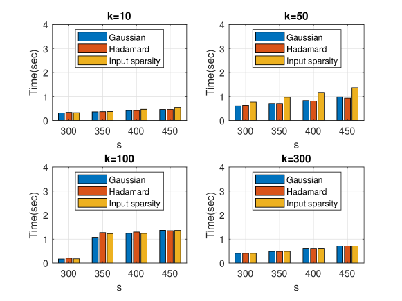
We generated random density matrices for most of which we used the QETLAB Matlab toolbox [12] to derive (real-valued) density matrices of size 5,000×5,000500050005,000\times 5,000, on which most of our extensive evaluations were run. We also tested our methods on a much larger 30,000×30,000300003000030,000\times 30,000 density matrix, which was close to the largest matrix that Matlab would allow us to load. We used the function RandomDensityMatrix of QETLAB and the Haar measure; we also experimented with the Bures measure to generate random matrices, but we did not observe any qualitative differences worth reporting. Recall that exactly computing the Von-Neumann entropy using eqn. (1) presumes knowledge of the entire spectrum of the matrix; to compute all singular values of a matrix we used the svd function of Matlab. The accuracy of our proposed approximation algorithms was evaluated by measuring the relative error; wall-clock times were reported in order to quantify the speedup that our approximation algorithms were able to achieve.

6.1 Empirical results for the Taylor and Chebyshev approximation algorithms

We start by reporting results on the Taylor and Chebyshev approximation algorithms, which have two sources of error: the number of terms that are retained in either the Taylor series expansion or the Chebyshev polynomial approximation and the trace estimation that is used in both approximation algorithms. We will separately evaluate the accuracy loss that is contributed by each source of error in order to understand the behavior of the proposed approximation algorithms.

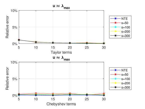
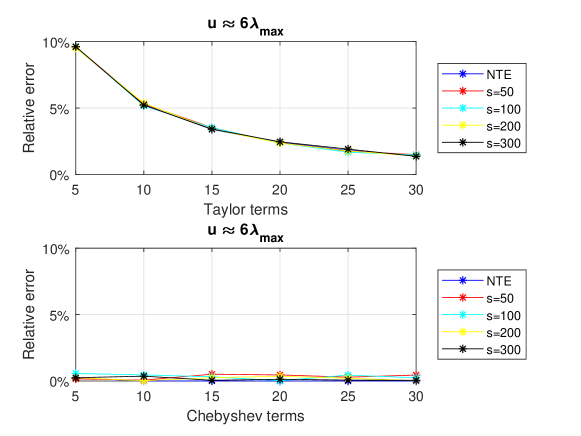
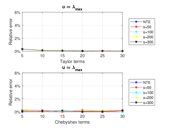
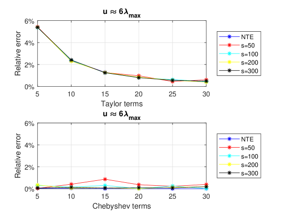
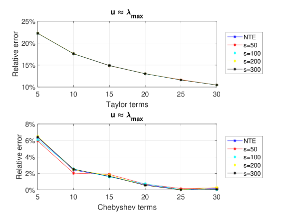
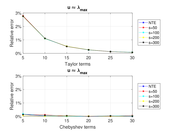
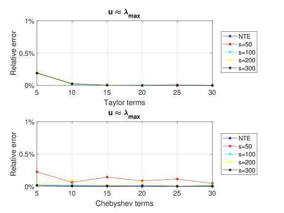
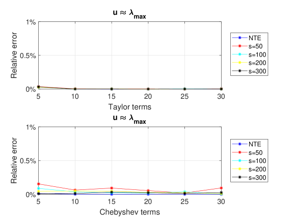
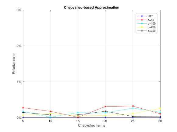
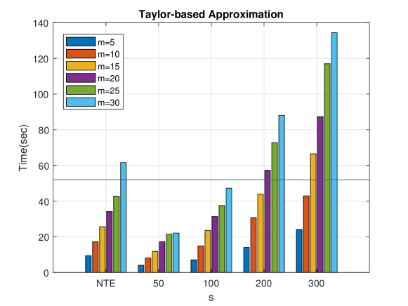
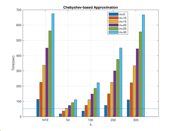
Consider a 5,000×5,000500050005,000\times 5,000 random density matrix and let m𝑚m (the number of terms retained in the Taylor series approximation or the degree of the polynomial used in the Chebyshev polynomial approximation) range between five and 30 in increments of five. Let s𝑠s, the number of random Gaussian vectors used to estimate the trace, be set to {50,100,200,300}50100200300\{50,100,200,300\}. Recall that our error bounds for Algorithms 1 and 2 depend on u𝑢u, an estimate for the largest eigenvalue of the density matrix. We used the power method to estimate the largest eigenvalue (let λ~maxsubscript~𝜆\tilde{\lambda}_{\max} be the estimate) and we set u𝑢u to λ~maxsubscript~𝜆\tilde{\lambda}_{\max} and 6λ~max6subscript~𝜆6\tilde{\lambda}_{\max}. Figures 1 and 2 show the relative error (out of 100%) for all combinations of m𝑚m, s𝑠s, and u𝑢u for the Taylor and Chebyshev approximation algorithms. It is worth noting that we also report the error when no trace estimation (NTE) is used in order to highlight that most of the accuracy loss is due to the Taylor/Chebyshev approximation and not the trace estimation.

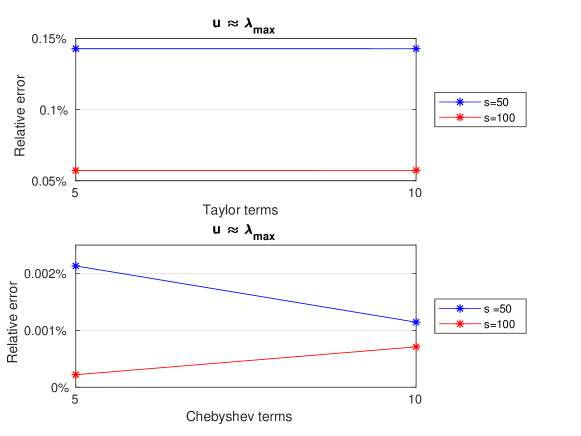
We observe that the relative error is always small, typically close to 111-2%percent22\%, for any choice of the parameters s𝑠s, m𝑚m, and u𝑢u. The Chebyshev algorithm returns better approximations when u𝑢u is an overestimate for λmaxsubscript𝜆\lambda_{\max} while the two algorithms are comparable (in terms of accuracy) where u𝑢u is very close to λmaxsubscript𝜆\lambda_{\max}, which agrees with our theoretical results. We also note that estimating the largest eigenvalue incurs minimal computational cost (less than one second). The NTE line (no trace estimation) in the plots serves as a lower bound for the relative error. Finally, we note that computing the exact Von-Neumann entropy took approximately 1.51.51.5 minutes for matrices of this size.

Refer to caption
Figure 1: Relative error for 5,000×5,000500050005,000\times 5,000 density matrix using the Taylor and the Chebyshev approximation algorithms with u=λ~max𝑢subscript~𝜆u=\tilde{\lambda}_{\max}.
Refer to caption
Figure 2: Relative error for 5,000×5,000500050005,000\times 5,000 density matrix using the Taylor and the Chebyshev approximation algorithms with u=6λ~max𝑢6subscript~𝜆u=6\tilde{\lambda}_{\max}.
Refer to caption
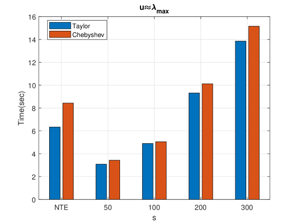
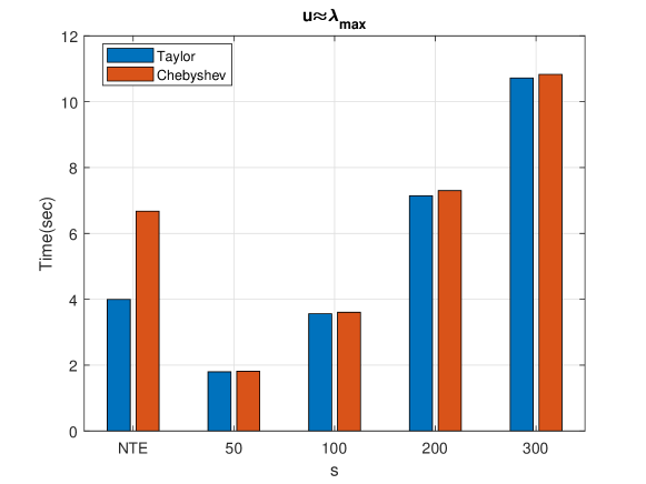
Figure 3: Time (in seconds) to run the approximate algorithms for the 5,000×5,000500050005,000\times 5,000 density matrix for m=5𝑚5m=5. Exactly computing the Von-Neumann entropy took approximately 90 seconds.

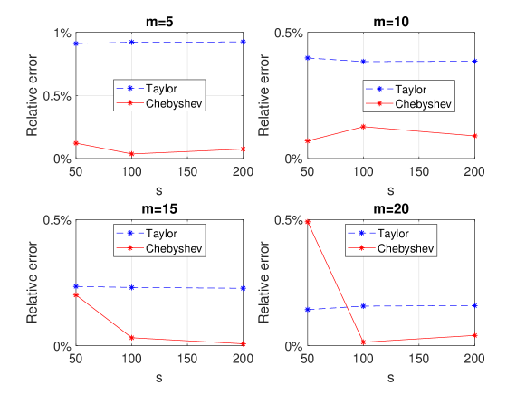
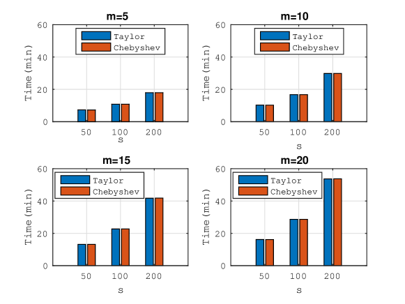
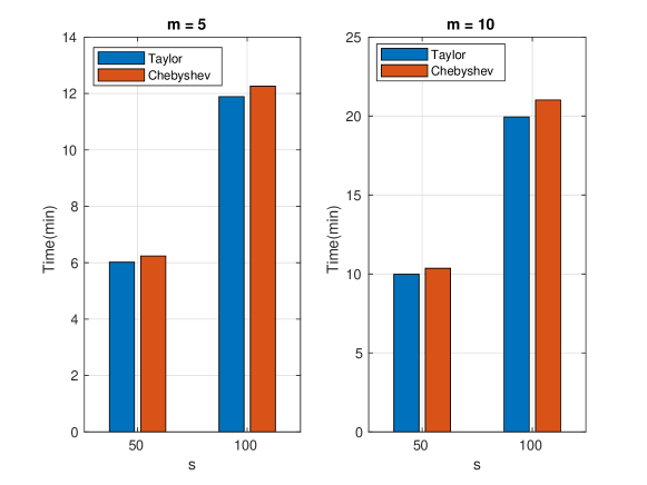
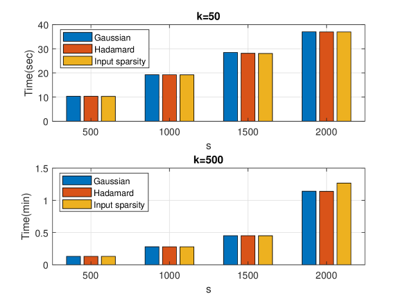
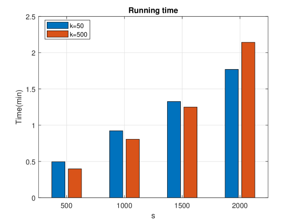
The second dataset that we experimented with was a much larger density matrix of size 30,000×30,000300003000030,000\times 30,000. This matrix was the largest matrix for which the memory was sufficient to perform operations like the full SVD. Notice that since the increase in the matrix size is six-fold compared to the previous one and SVD’s running time grows cubically with the input size, we expect the running time to compute the exact SVD to be roughly 6390superscript63906^{3}\cdot 90 seconds, which is approximately 5.4 hours; indeed, the exact computation of the Von-Neumann entropy took approximately 5.65.65.6 hours. We evaluated both the Taylor and the Chebyshev approximation schemes by setting the parameters m𝑚m and s𝑠s to take values in the sets {5,10,15,20}5101520\{5,10,15,20\} and {50,100,200}50100200\{50,100,200\}, respectively. The parameter u𝑢u was set to λ~maxsubscript~𝜆\tilde{\lambda}_{\max}, where the latter value was computed using the power method, which took approximately 3.63.63.6 minutes. We report the wall-clock running times and relative error (out of 100%) in Figures 5 and 4.

We observe that the relative error is always less than 1%percent11\% for both methods, with the Chebyshev approximation yielding almost always slightly better results. Note that our Chebyshev-polynomial-based approximation algorithm significantly outperformed the exact computation: e.g., for m=5𝑚5m=5 and s=50𝑠50s=50, our estimate was computed in less than ten minutes and achieved less than .2%percent.2.2\% relative error.

Refer to caption
Figure 4: Relative error for 30,000×30,000300003000030,000\times 30,000 density matrix using the Taylor and the Chebyshev approximation algorithms with u=λ~max𝑢subscript~𝜆u=\tilde{\lambda}_{\max}.
Refer to caption
Figure 5: Wall-clock times: Taylor approximation (blue) and Chebyshev approximation (red) for u=λ~max𝑢subscript~𝜆u=\tilde{\lambda}_{\max}. Exact computation needed approximately 5.6 hours.

The third dataset we experimented with was the tridiagonal matrix from [9, Section 5.1]:

𝐀=[2100121001210012]𝐀matrix2100121001210012\mathbf{A}=\begin{bmatrix}2&-1&0&\dots&0\\ -1&2&-1&\ddots&\vdots\\ 0&\ddots&\ddots&\ddots&0\\ \vdots&\ddots&-1&2&-1\\ 0&\dots&0&-1&2\\ \end{bmatrix} (21)

This matrix is the coefficient matrix of the discretized one-dimensional Poisson equation:

f(x)=d2vxdx𝑓𝑥superscript𝑑2subscript𝑣𝑥𝑑𝑥f(x)=-\frac{d^{2}v_{x}}{dx}

defined in the interval [0,1]01[0,1] with Dirichlet boundary conditions v(0)=v(1)=0𝑣0𝑣10v(0)=v(1)=0. We normalize 𝐀𝐀\mathbf{A} by dividing it with its trace in order to make it a density matrix. Consider the 5,000×5,000500050005,000\times 5,000 normalized matrix 𝐀𝐀\mathbf{A} and let m𝑚m (the number of terms retained in the Taylor series approximation or the degree of the polynomial used in the Chebyshev polynomial approximation) range between five and 30 in increments of five. Let s𝑠s, the number of random Gaussian vectors used for estimating the trace be set to 50, 100, 200, or 300. We used the formula

λi=42nsin2(iπ2n+2),i=1,,nformulae-sequencesubscript𝜆𝑖42𝑛superscript2𝑖𝜋2𝑛2𝑖1𝑛\lambda_{i}=\frac{4}{2n}\sin^{2}\left(\frac{i\pi}{2n+2}\right),\quad i=1,\dots,n (22)

to compute the eigenvalues of 𝐀𝐀\mathbf{A} (after normalization) and we set u𝑢u to λmaxsubscript𝜆{\lambda}_{\max} and 6λmax6subscript𝜆6{\lambda}_{\max}. Figures 6 and 7 show the relative error (out of 100%) for all combinations of m𝑚m, s𝑠s, and u𝑢u for the Taylor and Chebyshev approximation algorithms. We also report the error when no trace estimation (NTE) is used.

We observe that the relative error is higher than the one observed for the 5,000×5,000500050005,000\times 5,000 random density matrix. We report wall-clock running times in Figure 8. The Chebyshev-polynomial-based algorithm returns better approximations for all choices of the parameters and, in most cases, is faster than the Taylor-polynomial-based algorithm, e.g. for m=5𝑚5m=5, s=50𝑠50s=50 and u=λmax𝑢subscript𝜆u={\lambda}_{\max}, our estimate was computed in about two seconds and achieved less than .5%percent.5.5\% relative error.

Refer to caption
Figure 6: Relative error for 5,000×5,000500050005,000\times 5,000 tridiagonal density matrix using the Taylor and the Chebyshev approximation algorithms with u=λmax𝑢subscript𝜆u={\lambda}_{\max}.
Refer to caption
Figure 7: Relative error for 5,000×5,000500050005,000\times 5,000 tridiagonal density matrix using the Taylor and the Chebyshev approximation algorithms with u=6λmax𝑢6subscript𝜆u=6{\lambda}_{\max}.
Refer to caption
Figure 8: Wall-clock times: Taylor approximation (blue) and Chebyshev approximation (red) for m=5𝑚5m=5. Exact computation needed approximately 303030 seconds.

We further considered a 108×108superscript108superscript10810^{8}\times 10^{8} tridiagonal matrix of the form of eqn. (21). Although an exact computation of the singular values of 𝐀𝐀\mathbf{A} is not feasible (at least with our computational resources), such a computation is not necessary since eqn. (22) provides a closed formula for its eigenvalues and, thus, its entropy. Let m𝑚m (the number of terms retained in the Taylor series approximation or the degree of the polynomial used in the Chebyshev polynomial approximation) be equal to five or ten and let s𝑠s, the number of random Gaussian vectors used to estimate the trace be equal to 50 or 100. Figures 9 and 10 show the relative error (out of 100%) and the runtime, respectively, for all combinations of m𝑚m and s𝑠s for both the Taylor and Chebyshev approximation algorithms. We observe that in both cases we estimated the entropy in less than ten minutes with a relative error below 0.15%percent0.150.15\%.

Refer to caption
Figure 9: Relative error for the 108×108superscript108superscript10810^{8}\times 10^{8} tridiagonal density matrix using the Taylor and the Chebyshev approximation algorithms with u=λmax𝑢subscript𝜆u={\lambda}_{\max}.
Refer to caption
Figure 10: Wall-clock times: Taylor approximation (blue) and Chebyshev approximation (red) for the 108×108superscript108superscript10810^{8}\times 10^{8} triadiagonal density matrix. Exact computation using the Singular Value Decomposition was infeasible using our computational resources.

The fourth dataset we experimented with includes 5,000×5,000500050005,000\times 5,000 density matrices whose first top-k𝑘k eigenvalues follow a linear decay and the remaining 5,000k5000𝑘5,000-k a uniform distribution. Let k𝑘k, the number of eigenvalues that follow the linear decay, take values in the set {50, 1000, 3500, 5000}50100035005000\{50,\ 1000,\ 3500,\ 5000\}. Let m𝑚m, the number of terms retained in the Taylor series approximation or the degree of the polynomial used in the Chebyshev polynomial approximation, range between five and 30 in increments of five. Let s𝑠s, the number of random Gaussian vectors used to estimate the trace, be set to {50,100,200,300}50100200300\{50,100,200,300\}. The estimate of the largest eigenvalue u𝑢u is set to λ~maxsubscript~𝜆\tilde{\lambda}_{\max}. Figures 11 to 14 show the relative error (out of 100%) for all combinations of k𝑘k, m𝑚m, s𝑠s, and u𝑢u for the Taylor and Chebyshev approximation algorithms.

We observe that the relative error is decreasing as k𝑘k increases. It is worth noting that when k=3,500𝑘3500k=3,500 and k=5,000𝑘5000k=5,000 the Taylor-polynomial-based algorithm returns better relative error approximation than the Chebyshev-polynomial-based algorithm. In the latter case we observe that the relative error of the Taylor-based algorithm is almost zero. This observation has a simple explanation. Figure 15 shows the distribution of the eigenvalues in the four cases we examine. We observe that for k=50𝑘50k=50 the eigenvalues are spread in the interval (102,104)superscript102superscript104(10^{-2},10^{-4}); for k=1,000𝑘1000k=1,000 the eigenvalues are spread in the interval (103,104)superscript103superscript104(10^{-3},10^{-4}); while for k=3,500𝑘3500k=3,500 or k=5,000𝑘5000k=5,000 the eigenvalues are of order 104superscript10410^{-4}. It is well known that the Taylor polynomial returns highly accurate approximations when it is computed on values lying inside the open disc centered at a specific value u𝑢u, which, in our case, is the approximation to the dominant eigenvalue. The radius of the disk is roughly r=λm+1/λm𝑟subscript𝜆𝑚1subscript𝜆𝑚r=\lambda_{m+1}/\lambda_{m}, where m𝑚m is the degree of the Taylor polynomial. If r1𝑟1r\leq 1 then the Taylor polynomial converges; otherwise it diverges. Figure 16 shows the convergence rate for various values of k𝑘k. We observe that for k=50𝑘50k=50 the polynomial diverges, which leads to increased errors for the Taylor-based approximation algorithm (reported error close to 23%percent2323\%). In all other cases, the convergence rate is close to one, resulting in negligible impact to the overall error.

In all four cases, the Chebyshev-polynomial based algorithm behaves better or similar to the Taylor-polynomial based algorithm. It is worth noting that when the majority of the eigenvalues are clustered around the smallest eigenvalue, then to achieve relative error similar to the one observed for the QETLAB random density matrices, more than 303030 polynomial terms need to be retained, which increases the computational time of our algorithms. The increase of the computational time as well as the increased relative error can be justified by the large condition number that these matrices have (remember that for both approximation algorithms the running time depends on the approximate condition number u/l𝑢𝑙u/l). As an example, for k=50𝑘50k=50, the condition number is in the order of hundreds which is significant larger than the roughly constant condition number when k=5,000𝑘5000k=5,000.

Refer to caption
Figure 11: Relative error for 5,000×5,000500050005,000\times 5,000 density matrix with the top-505050 eigenvalues decaying linearly using the Taylor and the Chebyshev approximation algorithms with u=λmax𝑢subscript𝜆u={\lambda}_{\max}.
Refer to caption
Figure 12: Relative error for 5,000×5,000500050005,000\times 5,000 density matrix with the top-100010001000 eigenvalues decaying linearly using the Taylor and the Chebyshev approximation algorithms with u=λmax𝑢subscript𝜆u={\lambda}_{\max}.
Refer to caption
Figure 13: Relative error for 5,000×5,000500050005,000\times 5,000 density matrix with the top-350035003500 eigenvalues decaying linearly using the Taylor and the Chebyshev approximation algorithms with u=λmax𝑢subscript𝜆u={\lambda}_{\max}.
Refer to caption
Figure 14: Relative error for 5,000×5,000500050005,000\times 5,000 density matrix with the top-500050005000 eigenvalues decaying linearly using the Taylor and the Chebyshev approximation algorithms with u=λmax𝑢subscript𝜆u={\lambda}_{\max}.
Refer to caption
Figure 15: Eigenvalue distribution of 5,000×5,000500050005,000\times 5,000 density matrices with the top-k={50, 1000, 3500, 5000}𝑘50100035005000k=\{50,\ 1000,\ 3500,\ 5000\} eigenvalues decaying linearly and the remaining ones (5,000k5000𝑘5,000-k) following a uniform distribution.
Refer to caption
Figure 16: Convergence radius of the Taylor polynomial for the 5,000×5,000500050005,000\times 5,000 density matrices with the top-k={50, 1000, 3500, 5000}𝑘50100035005000k=\{50,\ 1000,\ 3500,\ 5000\} eigenvalues decaying linearly and the remaining ones (5,000k5000𝑘5,000-k) following a uniform distribution.

6.2 Empirical Results for the Hermitian Case

Our last dataset is a random 5,000×5,000500050005,000\times 5,000 complex density matrix generated using the QETLAB Matlab toolbox. We used the function RandomDensityMatrix of QETLAB and the Haar measure. Let m𝑚m (the number of terms retained in the Taylor series approximation or the degree of the polynomial used in the Chebyshev polynomial approximation) range between five and 30 in increments of five. Let s𝑠s, the number of random Gaussian vectors used to estimate the trace, be set to {50,100,200,300}50100200300\{50,100,200,300\}. Figures 17 and 18 show the relative error (out of 100%) for all combinations of m𝑚m, s𝑠s, and u𝑢u for the Taylor-based and Chebyshev-based approximation algorithms respectively.

We observe that the relative error is always small, typically below 1%percent11\%, for any choice of the parameters s𝑠s and m𝑚m. The NTE line (no trace estimation) in the plots serves as a lower bound for the relative error. We note that computing the exact Von-Neumann entropy took approximately 525252 seconds for matrices of this size. Finally, our algorithm seems to outperform exact computation of the von-Neumann entropy by approximating it in about ten seconds (for the Taylor-based approach) with a relative error of 0.5%percent0.50.5\% using 100100100 random Gaussian vectors and retaining ten Taylor terms (see Fig. 19) or in about 181818 seconds (for the Chebyshev-based approach) with a relative error of 0.2%percent0.20.2\% using 505050 random Gaussian vectors and five Chebyshev polynomials (see Fig.20) .
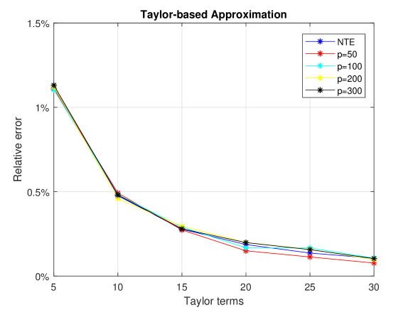
Refer to caption
Figure 17: Relative error for 5,000×5,000500050005,000\times 5,000 density matrix using the Taylor approximation algorithm.
Refer to caption
Figure 18: Relative error for 5,000×5,000500050005,000\times 5,000 density matrix using the Chebyshev approximation algorithm.
Refer to caption
Figure 19: Time (in seconds) to run the Taylor-based algorithm for the 5,000×5,000500050005,000\times 5,000 density matrix for all combinations of m𝑚m and s𝑠s. Exactly computing the Von-Neumann entropy took approximately 52 seconds, designated by the straight horizontal line in the figure.
Refer to caption
Figure 20: Time (in seconds) to run the Chebyshev-based algorithm for the 5,000×5,000500050005,000\times 5,000 density matrix for all combinations of m𝑚m and s𝑠s. Exactly computing the Von-Neumann entropy took approximately 52 seconds, designated by the straight horizontal line in the figure.

6.3 Empirical results for the random projection approximation algorithms

In order to evaluate our third algorithm, we generated low-rank random density matrices (recall that the algorithm of Section 5 works only for random density matrices of rank k𝑘k with knmuch-less-than𝑘𝑛k\ll n). Additionally, in order to evaluate the subsampled randomized Hadamard transform and avoid padding with all-zero rows, we focused on values of n𝑛n (the number of rows and columns of the density matrix) that are powers of two. Finally, we also evaluated a simpler random projection matrix, namely the Gaussian random matrix, whose entries are all Gaussian random variables with zero mean and unit variance.

We generated low rank random density matrices with exponentially (using the QETLAB Matlab toolbox) and linearly decaying eigenvalues. The sizes of the density matrices we tested were 4,096×4,096409640964,096\times 4,096 and 16,384×16,384163841638416,384\times 16,384. We also generated much larger 30,000×30,000300003000030,000\times 30,000 random matrices on which we only experimented with the Gaussian random projection matrix.

We computed all the non-zero singular values of a matrix using the svds function of Matlab in order to take advantage of the fact that the target density matrix has low rank. The accuracy of our proposed approximation algorithms was evaluated by measuring the relative error; wall-clock times were reported in order to quantify the speedup that our approximation algorithms were able to achieve.

We start by reporting results for Algorithm 5 using the Gaussian, the subsampled randomized Hadamard transform (Algorithm 6), and the input-sparsity transform (Algorithm 7) random projection matrices. Consider the 4,096×4,096409640964,096\times 4,096 low rank density matrices and let k𝑘k, the rank of the matrix, be 101010, 505050, 100100100, and 300300300. Let s𝑠s, the number of columns of the random projection matrix, range from 505050 to 1,00010001,000 in increments of 505050. Figures 21 and 22 depict the relative error (out of 100%percent100100\%) for all combinations of k𝑘k and s𝑠s. We also report the wall-clock running times for values of s𝑠s between 300300300 and 450450450 at Figure 23.

We observe that in the case of the random matrix with exponentially decaying eigenvalues and for all algorithms the relative error is under 0.3%percent0.30.3\% for any choice of the parameters k𝑘k and s𝑠s and, as expected, decreases as the dimension of the projection space s𝑠s grows larger. Interestingly, all three random projection matrices returned essentially identical accuracies and very comparable wall-clock running time results. This observation is due to the fact that for all choices of k𝑘k, after scaling the matrix to unit trace, the only eigenvalues that were numerically non-zero were the 101010 dominant ones.

In the case of the random matrix with linearly decaying eigenvalues (and for all algorithms) the relative error increases as the rank of the matrix increases and decreases as the size of the random projection matrix increases. This is expected: as the rank of the matrix increases, a larger random projection space is needed to capture the “energy” of the matrix. Indeed, we observe that for all values of k𝑘k, setting s=1,000𝑠1000s=1,000 guarantees a relative error under 1%percent11\%. Similarly, for k=10𝑘10k=10, the relative error is under 0.3%percent0.30.3\% for any choice of s𝑠s.

The running time depends not only on the size of the matrix, but also on its rank, e.g. for k=100𝑘100k=100 and s=450𝑠450s=450, our approximation was computed in about 2.52.52.5 seconds, whereas for k=300𝑘300k=300 and s=450𝑠450s=450, it was computed in less than one second. Considering, for example, the case of k=300𝑘300k=300 exponentially decaying eigenvalues, we observe that for s=400𝑠400s=400 we achieve relative error below 0.150.150.15% and a speedup of over 606060 times compared to the exact computation. Finally, it is observed that all three algorithms returned very comparable wall-clock running time results. This observation could be due to the fact that matrix multiplication is heavily optimized in Matlab and therefore the theoretical advantages of the Hadamard transform did not manifest themselves in practice.
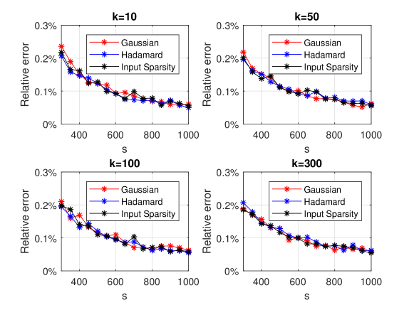
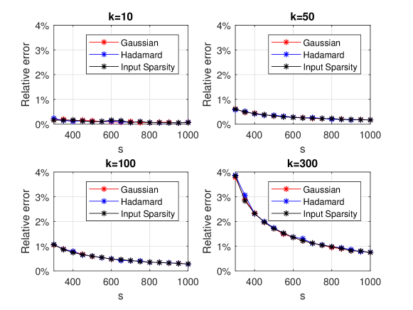
Refer to caption
Figure 21: Relative error for the 4,096×4,096409640964,096\times 4,096 rank-k𝑘k density matrix with exponentially decaying eigenvalues using Algorithm 5 with the Gaussian (red), the subsampled randomized Hadamard transform (blue), and the input sparsity transform (black) random projection matrices.
Refer to caption
Figure 22: Relative error for the 4,096×4,096409640964,096\times 4,096 rank-k𝑘k density matrix with linearly decaying eigenvalues using Algorithm 5 with the Gaussian (red), the subsampled randomized Hadamard transform (blue), and the input sparsity transform (black) random projection matrices.
Refer to caption
Figure 23: Wall-clock times: Algorithm 5 on 4,096×4,096409640964,096\times 4,096 random matrices, with the Gaussian (blue), the subsampled randomized Hadamard transform (red) and the input sparsity transform (orange) projection matrices. The exact entropy was computed in 1.51.51.5 seconds for the rank-10 approximation, in eight seconds for the rank-50 approximation, in 151515 seconds for the rank-100 approximation, and in one minute for the rank-300 approximation.

The second dataset we experimented with was a 16,384×16,384163841638416,384\times 16,384 low rank density matrix. We set k=50𝑘50k=50 and k=500𝑘500k=500 and we let s𝑠s take values in the set {500, 1000, 1500,,3000, 3500}5001000150030003500\{500,\ 1000,\ 1500,\ldots,3000,\ 3500\}. We report the relative error (out of 100%percent100100\%) for all combinations of k𝑘k and s𝑠s in Figure 24 for the matrix with exponentially decaying eigenvalues and in Figure 25 for the matrix with linearly decaying eigenvalues. We also report the wall-clock running times for s𝑠s between 500500500 and 2,00020002,000 in Figure 26. We observe that the relative error is typically around 1%percent11\% for both types of matrices, with running times ranging between ten seconds and four minutes, significantly outperforming the exact entropy computation which took approximately 1.61.61.6 minutes for the rank 50 approximation and 20 minutes for the rank 500 approximation.
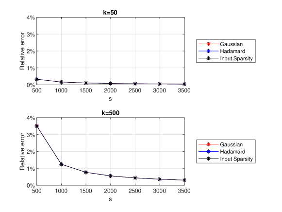
Refer to caption
Figure 24: Relative error for the 16,384×16,384163841638416,384\times 16,384 rank-k𝑘k density matrix with exponentially decaying eigenvalues using Algorithm 5 with the Gaussian (red), the subsampled randomized Hadamard transform (blue), and the input sparsity transform (black) random projection matrices.
Refer to caption
Figure 25: Relative error for the 16,384×16,384163841638416,384\times 16,384 rank-k𝑘k density matrix with linearly decaying eigenvalues using Algorithm 5 with the Gaussian (red), the subsampled randomized Hadamard transform (blue), and the input sparsity transform (black) random projection matrices.
Refer to caption
Figure 26: Wall-clock times: Algorithm 5 with the Gaussian (blue), the subsampled randomized Hadamard transform (red) and the input sparsity transform (orange) projection matrices. The exact entropy was computed in 1.61.61.6 minutes for the rank 50 approximation and in 202020 minutes for the rank 500 approximation.
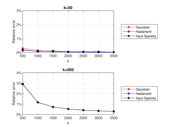
The last dataset we experimented with was a 30,000×30,000300003000030,000\times 30,000 low rank density matrix on which we ran Algorithm 5 using a Gaussian random projection matrix. We set k=50𝑘50k=50 and k=500𝑘500k=500 and we let s𝑠s take values in the set {500, 1000, 1500,,3000, 3500}5001000150030003500\{500,\ 1000,\ 1500,\ldots,3000,\ 3500\}. We report the relative error (out of 100%percent100100\%) for all combinations of k𝑘k and s𝑠s in Figure 27 for the matrix with exponentially decaying eigenvalues and in Figure 28 for the matrix with the linearly decaying eigenvalues. We also report the wall-clock running times for s𝑠s ranging between 500500500 and 2,00020002,000 in Figure 29. We observe that the relative error is typically around 1%percent11\% for both types of matrices, with the running times ranging between 303030 seconds and two minutes, outperforming the exact entropy which was computed in six minutes for the rank 50 approximation and in one hour for the rank 500 approximation.
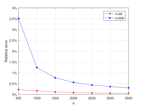
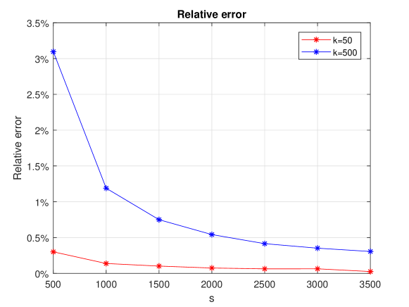
Refer to caption
Figure 27: Relative error for the 30,000×30,000300003000030,000\times 30,000 rank-k𝑘k density matrix with exponentially decaying eigenvalues using Algorithm 5 with the Gaussian random projection matrix for k=50𝑘50k=50 (red) and for k=500𝑘500k=500 (blue).
Refer to caption
Figure 28: Relative error for the 30,000×30,000300003000030,000\times 30,000 rank-k𝑘k density matrix with linearly decaying eigenvalues using Algorithm 5 with the Gaussian random projection matrix for k=50𝑘50k=50 (red) and for k=500𝑘500k=500 (blue).
Refer to caption
Figure 29: Wall-clock times: rank-50 approximation (blue) and rank-500 approximation (red). Exact computation needed about six minutes and one hour respectively.

7 Conclusions and open problems

We presented and analyzed three randomized algorithms to approximate the von Neumann entropy of density matrices. Our algorithms leverage recent developments in the RandNLA literature: randomized trace estimators, provable bounds for the power method, the use of random projections to approximate the singular values of a matrix, etc. All three algorithms come with provable accuracy guarantees under assumptions on the spectrum of the density matrix. Empirical evaluations on 30,000×30,000300003000030,000\times 30,000 synthetic density matrices support our theoretical findings and demonstrate that we can efficiently approximate the von Neumann entropy in a few minutes with minimal loss in accuracy, whereas an the exact computation takes over 5.5 hours.

An interesting open problem would be to consider the estimation of the cross entropy. The cross entropy is a measure between two probability distributions and is particularly important in information theory. Algebraically, it can be defined as (𝐒,𝐑)=tr(𝐒log𝐑)𝐒𝐑tr𝐒𝐑\mathcal{H}\left(\mathbf{S},\mathbf{R}\right)=-\mathrm{\textbf{\rm\bf tr}}\left(\mathbf{S}\log{\mathbf{R}}\right), where 𝐒n×n𝐒superscript𝑛𝑛\mathbf{S}\in\mathbb{C}^{n\times n} and 𝐑n×n𝐑superscript𝑛𝑛\mathbf{R}\in\mathbb{C}^{n\times n} are density matrices with a full set of pure states. One can further extend our polynomial-based approaches using the Taylor expansion or the Chebyshev polynomials to approximate the matrix Γ=𝐒log𝐑Γ𝐒𝐑\Gamma=\mathbf{S}\log\mathbf{R}. The case where both or one of the density matrices have an incomplete set of pure states is an open problem: if 𝐑𝐑\mathbf{R} is low-rank, then our first two approaches would not work for the reasons discussed in Section 5. However, if the only low rank matrix is 𝐒𝐒\mathbf{S}, then our first two approaches would still work: 𝐒𝐒\mathbf{S} is only appearing in the trace estimation part, and having eigenvalues equal to zero does not affect the positive semi-definiteness of ΓΓ\Gamma. When 𝐑𝐑\mathbf{R} is of low rank then one might be able to use our random projection approaches to reduce its dimensionality and/or the dimensionality of 𝐒𝐒\mathbf{S}.

The most important open problem is to relax (or eliminate) the assumptions associated with our three key technical results without sacrificing our running time guarantees. It would be critical to understand whether our assumptions are, for example, necessary to achieve relative error approximations and either provide algorithmic results that relax or eliminate our assumptions or provide matching lower bounds and counterexamples.

References

  • [1] Nir Ailon and Bernard Chazelle. The Fast Johnson–Lindenstrauss Transform and Approximate Nearest Neighbors. SIAM Journal on Computing, 39(1):302–322, 2009.
  • [2] Haim Avron and Sivan Toledo. Randomized Algorithms for Estimating the Trace of an Implicit Symmetric Positive Semi-definite Matrix. Journal of the ACM, 58(2):8, 2011.
  • [3] Christos Boutsidis, Petros Drineas, Prabhanjan Kambadur, Eugenia-Maria Kontopoulou, and Anastasios Zouzias. A Randomized Algorithm for Approximating the Log Determinant of a Symmetric Positive Definite Matrix. Linear Algebra and its Applications, 533:95–117, 2017.
  • [4] Kenneth L. Clarkson and David P. Woodruff. Low Rank Approximation and Regression in Input Sparsity Time. In Proceedings of the 45th annual ACM Symposium on Theory of Computing, pages 81–90. ACM Press, 2013.
  • [5] James Demmel and Kresimir Veselic. Jacobi’s Method is more Accurate than QR. SIAM Journal on Matrix Analysis and Applications, 13(4):1204–1245, 1992.
  • [6] Petros Drineas and Michael W. Mahoney. RandNLA: Randomized Numerical Linear Algebra. Communications of the ACM, 59(6):80–90, 2016.
  • [7] Petros Drineas, Michael W. Mahoney, S Muthukrishnan, and Tamás Sarlós. Faster Least Squares Approximation. Numerische Mathematik, 117:219–249, 2011.
  • [8] Gene H. Golub and Charles F. Van Loan. Matrix Computations (3rd Ed.). Johns Hopkins University Press, Baltimore, MD, USA, 1996.
  • [9] Insu Han, Dmitry Malioutov, and Jinwoo Shin. Large-scale Log-determinant Computation through Stochastic Chebyshev Expansions. Proceedings of the 32nd International Conference on Machine Learning, 37:908–917, 2015.
  • [10] Nicholas JA Harvey, Jelani Nelson, and Krzysztof Onak. Sketching and streaming entropy via approximation theory. In IEEE Annual Symposium on Foundations of Computer Science, pages 489–498, 2008.
  • [11] Nicholas J. Higham. Functions of Matrices: Theory and Computation. Society for Industrial and Applied Mathematics, Philadelphia, PA, USA, 2008.
  • [12] Nathaniel Johnston. QETLAB: A Matlab toolbox for quantum entanglement, version 0.9. http://qetlab.com, 2016.
  • [13] Xiangrui Meng and Michael W. Mahoney. Low-distortion Subspace Embeddings in Input-sparsity Time and Applications to Robust Linear Regression. In Proceedings of the 45th annual ACM Symposium on Theory of Computing, pages 91–100, 2013.
  • [14] Cameron Musco, Praneeth Netrapalli, Aaron Sidford, Shashanka Ubaru, and David P. Woodruff. Spectrum Approximation Beyond Fast Matrix Multiplication: Algorithms and Hardness. 2018.
  • [15] Jelani Nelson and Huy L. Nguyễn. OSNAP: Faster Numerical Linear Algebra Algorithms via Sparser Subspace Embeddings. In Proceedings of the 46th annual IEEE Symposium on Foundations of Computer Science, 2013.
  • [16] Saurabh Paul, Christos Boutsidis, Malik Magdon-Ismail, and Petros Drineas. Random projections and support vector machines. In Proceeding of the 16th International Conference on Artificial Intelligence and Statistics, 2013.
  • [17] Luca Trevisan. Graph Partitioning and Expanders. Handout 7, 2011.
  • [18] Joel A. Tropp. Improved Analysis of the Subsampled Randomized Hadamard Transform. Advances in Adaptive Data Analysis, 03(01):8, 2010.
  • [19] Thomas P. Wihler, Banz Bessire, and Andre Stefanov. Computing the Entropy of a Large Matrix. Journal of Physics A: Mathematical and Theoretical, 47(24):245201, 2014.
  • [20] David P. Woodruff. Sketching as a Tool for Numerical Linear Algebra. Foundations and Trends in Theoretical Computer Science, 10(1-2):1–157, 2014.

8 The power method

We consider the well-known power method to estimate the largest eigenvalue of a matrix. In our context, we will use the power method to estimate the largest probability pisubscript𝑝𝑖p_{i} for a density matrix 𝐑𝐑\mathbf{R}.

  • INPUT: SPD matrix 𝐀n×n,𝐀superscript𝑛𝑛\mathbf{A}\in\mathbb{R}^{n\times n}, integers q,t>0𝑞𝑡0q,\ t>0.

  • For j=1,,q𝑗1𝑞j=1,\dots,q

    1. 1.

      Pick uniformly at random a vector 𝐱0j{+1,1}nsuperscriptsubscript𝐱0𝑗superscript11𝑛\mathbf{x}_{0}^{j}\in\{+1,-1\}^{n}.

    2. 2.

      For i=1,,t𝑖1𝑡i=1,\dots,t

      • \bullet

        𝐱ij=𝐀𝐱i1jsuperscriptsubscript𝐱𝑖𝑗𝐀subscriptsuperscript𝐱𝑗𝑖1\mathbf{x}_{i}^{j}=\mathbf{A}\cdot\mathbf{x}^{j}_{i-1}.

    3. 3.

      Compute: p~1j=𝐱tjT𝐀𝐱tj𝐱tjT𝐱tjsuperscriptsubscript~𝑝1𝑗superscriptsuperscriptsubscript𝐱𝑡𝑗𝑇superscriptsubscript𝐀𝐱𝑡𝑗superscriptsuperscriptsubscript𝐱𝑡𝑗𝑇superscriptsubscript𝐱𝑡𝑗\tilde{p}_{1}^{j}=\frac{{\mathbf{x}_{t}^{j}}^{T}\mathbf{A}\mathbf{x}_{t}^{j}}{{\mathbf{x}_{t}^{j}}^{T}\mathbf{x}_{t}^{j}}.

  • OUTPUT: p~1=maxj=1qp~1jsubscript~𝑝1subscript𝑗1𝑞superscriptsubscript~𝑝1𝑗\tilde{p}_{1}=\max_{j=1\ldots q}\tilde{p}_{1}^{j}.

Algorithm 8 Power method, repeated q𝑞q times.

Algorithm 8 requires 𝒪(qt(n+nnz(𝐀)))𝒪𝑞𝑡𝑛nnz𝐀\mathcal{O}(qt(n+\mathrm{nnz}(\mathbf{A}))) arithmetic operations to compute p~1subscript~𝑝1\tilde{p}_{1}. The following lemma appeared in [3], building upon [17].

Lemma 14.

Let p~1subscript~𝑝1\tilde{p}_{1} be the output of Algorithm 8 with q=4.82log(1/δ)𝑞4.821𝛿q=\left\lceil 4.82\log(1/\delta)\right\rceil and t=log4n𝑡4𝑛t=\left\lceil\log\sqrt{4n}\right\rceil. Then, with probability at least 1δ1𝛿1-\delta,

16p1p~1p1.16subscript𝑝1subscript~𝑝1subscript𝑝1\frac{1}{6}p_{1}\leq\tilde{p}_{1}\leq p_{1}.

The running time of Algorithm 8 is 𝒪((n+nnz(𝐀))log(n)log(1δ)).𝒪𝑛nnz𝐀𝑛1𝛿\mathcal{O}\left(\left(n+\mathrm{nnz}(\mathbf{A})\right)\log(n)\log\left(\frac{1}{\delta}\right)\right).

9 The Clenshaw Algorithm

We briefly sketch Clenshaw’s algorithm to evaluate Chebyshev polynomials with matrix inputs. Clenshaw’s algorithm is a recursive approach with base cases bm+2(x)=bm+1(x)=0subscript𝑏𝑚2𝑥subscript𝑏𝑚1𝑥0b_{m+2}(x)=b_{m+1}(x)=0 and the recursive step (for k=m,m1,,0𝑘𝑚𝑚10k=m,m-1,\ldots,0):

bk(x)=αk+2xbk+1(x)bk+2(x).subscript𝑏𝑘𝑥subscript𝛼𝑘2𝑥subscript𝑏𝑘1𝑥subscript𝑏𝑘2𝑥b_{k}(x)=\alpha_{k}+2xb_{k+1}(x)-b_{k+2}(x). (23)

(See Section 3 for the definition of αksubscript𝛼𝑘\alpha_{k}.) Then,

fm(x)=12(α0+b0(x)b2(x)).subscript𝑓𝑚𝑥12subscript𝛼0subscript𝑏0𝑥subscript𝑏2𝑥f_{m}(x)=\frac{1}{2}\left(\alpha_{0}+b_{0}(x)-b_{2}(x)\right). (24)

Using the mapping x2(x/u)1𝑥2𝑥𝑢1x\rightarrow 2(x/u)-1, eqn. (23) becomes

bk(x)=αk+2(2ux1)bk+1(x)bk+2(x).subscript𝑏𝑘𝑥subscript𝛼𝑘22𝑢𝑥1subscript𝑏𝑘1𝑥subscript𝑏𝑘2𝑥b_{k}(x)=\alpha_{k}+2\left(\frac{2}{u}x-1\right)b_{k+1}(x)-b_{k+2}(x). (25)

In the matrix case, we substitute x𝑥x by a matrix. Therefore, the base cases are 𝐁m+2(𝐑)=𝐁m+1(𝐑)=𝟎subscript𝐁𝑚2𝐑subscript𝐁𝑚1𝐑0\mathbf{B}_{m+2}(\mathbf{R})=\mathbf{B}_{m+1}(\mathbf{R})=\mathbf{0} and the recursive step is

𝐁k(𝐑)=αk𝐈n+2(2u𝐑𝐈n)𝐁k+1(𝐑)𝐁k+2(𝐑)subscript𝐁𝑘𝐑subscript𝛼𝑘subscript𝐈𝑛22𝑢𝐑subscript𝐈𝑛subscript𝐁𝑘1𝐑subscript𝐁𝑘2𝐑\mathbf{B}_{k}(\mathbf{R})=\alpha_{k}\mathbf{I}_{n}+2\left(\frac{2}{u}\mathbf{R}-\mathbf{I}_{n}\right)\mathbf{B}_{k+1}(\mathbf{R})-\mathbf{B}_{k+2}(\mathbf{R}) (26)

for k=m,m1,,0𝑘𝑚𝑚10k=m,m-1,\ldots,0. The final sum is

fm(𝐑)=12(α0𝐈n+𝐁0(𝐑)𝐁2(𝐑)).subscript𝑓𝑚𝐑12subscript𝛼0subscript𝐈𝑛subscript𝐁0𝐑subscript𝐁2𝐑f_{m}(\mathbf{R})=\frac{1}{2}\left(\alpha_{0}\mathbf{I}_{n}+\mathbf{B}_{0}(\mathbf{R})-\mathbf{B}_{2}(\mathbf{R})\right). (27)

Using the matrix version of Clenshaw’s algorithm, we can now rewrite the trace estimation 𝐠fm(𝐑)𝐠superscript𝐠topsubscript𝑓𝑚𝐑𝐠\mathbf{g}^{\top}f_{m}(\mathbf{R})\mathbf{g} as follows. First, we right multiply eqn. (26) by 𝐠𝐠\mathbf{g},

𝐁k(𝐑)𝐠subscript𝐁𝑘𝐑𝐠\displaystyle\mathbf{B}_{k}(\mathbf{R})\mathbf{g} =\displaystyle= αk𝐈n𝐠+2(2u𝐑𝐈n)𝐁k+1(𝐑)𝐠𝐁k+2(𝐑)𝐠,subscript𝛼𝑘subscript𝐈𝑛𝐠22𝑢𝐑subscript𝐈𝑛subscript𝐁𝑘1𝐑𝐠subscript𝐁𝑘2𝐑𝐠\displaystyle\alpha_{k}\mathbf{I}_{n}\mathbf{g}+2\left(\frac{2}{u}\mathbf{R}-\mathbf{I}_{n}\right)\mathbf{B}_{k+1}(\mathbf{R})\mathbf{g}-\mathbf{B}_{k+2}(\mathbf{R})\mathbf{g},
𝐲ksubscript𝐲𝑘\displaystyle\mathbf{y}_{k} =\displaystyle= αk𝐠+2(2u𝐑𝐈n)𝐲k+1𝐲k+2.subscript𝛼𝑘𝐠22𝑢𝐑subscript𝐈𝑛subscript𝐲𝑘1subscript𝐲𝑘2\displaystyle\alpha_{k}\mathbf{g}+2\left(\frac{2}{u}\mathbf{R}-\mathbf{I}_{n}\right)\mathbf{y}_{k+1}-\mathbf{y}_{k+2}. (28)

Eqn. (28) follows by substituting 𝐲i=𝐁i(𝐑)𝐠subscript𝐲𝑖subscript𝐁𝑖𝐑𝐠\mathbf{y}_{i}=\mathbf{B}_{i}(\mathbf{R})\mathbf{g}. Multiplying the base cases by 𝐠𝐠\mathbf{g}, we get 𝐲m+2=𝐲m+1=𝟎subscript𝐲𝑚2subscript𝐲𝑚10\mathbf{y}_{m+2}=\mathbf{y}_{m+1}=\mathbf{0} and the final sum becomes

𝐠fm(𝐑)𝐠=12(α0(𝐠𝐠)+𝐠(𝐲0𝐲2)).superscript𝐠topsubscript𝑓𝑚𝐑𝐠12subscript𝛼0superscript𝐠top𝐠superscript𝐠topsubscript𝐲0subscript𝐲2\mathbf{g}^{\top}f_{m}(\mathbf{R})\mathbf{g}=\frac{1}{2}\left(\alpha_{0}(\mathbf{g}^{\top}\mathbf{g})+\mathbf{g}^{\top}(\mathbf{y}_{0}-\mathbf{y}_{2})\right). (29)

Algorithm 9 summarizes all the above.

1:  INPUT: αisubscript𝛼𝑖\alpha_{i}i=0,,m𝑖0𝑚i=0,\dots,m, 𝐑n×n\mathbf{R}\in{}^{n\times n}, 𝐠n\mathbf{g}\in{}^{n}
2:  Set 𝐲m+2=𝐲m+1=𝟎subscript𝐲𝑚2subscript𝐲𝑚10\mathbf{y}_{m+2}=\mathbf{y}_{m+1}=\mathbf{0}
3:  for k=m,m1,,0𝑘𝑚𝑚10k=m,m-1,\ldots,0  do
4:     𝐲k=αk𝐠+4u𝐑𝐲k+12𝐲k+1𝐲k+2subscript𝐲𝑘subscript𝛼𝑘𝐠4𝑢subscript𝐑𝐲𝑘12subscript𝐲𝑘1subscript𝐲𝑘2\mathbf{y}_{k}=\alpha_{k}\mathbf{g}+\frac{4}{u}\mathbf{R}\mathbf{y}_{k+1}-2\mathbf{y}_{k+1}-\mathbf{y}_{k+2}
5:  end for
6:  OUTPUT: 𝐠fm(𝐑)𝐠=12(α0(𝐠𝐠)+𝐠(𝐲0𝐲2))superscript𝐠topsubscript𝑓𝑚𝐑𝐠12subscript𝛼0superscript𝐠top𝐠superscript𝐠topsubscript𝐲0subscript𝐲2\mathbf{g}^{\top}f_{m}(\mathbf{R})\mathbf{g}=\frac{1}{2}\left(\alpha_{0}(\mathbf{g}^{\top}\mathbf{g})+\mathbf{g}^{\top}(\mathbf{y}_{0}-\mathbf{y}_{2})\right)
Algorithm 9 Clenshaw’s algorithm to compute 𝐠fm(𝐑)𝐠superscript𝐠topsubscript𝑓𝑚𝐑𝐠\mathbf{g}^{\top}f_{m}(\mathbf{R})\mathbf{g}.