Counter-streaming flows in a giant quiet-Sun filament observed in the extreme ultraviolet

Abstract

Aims. The giant solar filament was visible on the solar surface from 2011 November 8 – 23. Multiwavelength data from the Solar Dynamics Observatory (SDO) were used to examine counter-streaming flows within the spine of the filament.

Methods. We use data from two SDO instruments, the Atmospheric Imaging Assembly (AIA) and the Helioseismic and Magnetic Imager (HMI), covering the whole filament, which stretched over more than half a solar diameter. H$\alpha$ images from the Kanzelhöhe Solar Observatory (KSO) provide context information of where the spine of the filament is defined and the barbs are located. We apply local correlation tracking (LCT) to a two-hour time series on 2011 November 16 of the AIA images to derive horizontal flow velocities of the filament. To enhance the contrast of the AIA images, noise adaptive fuzzy equalization (NAFE) is employed, which allows us to identify and quantify counter-streaming flows in the filament. We observe the same cool filament plasma in absorption in both H$\alpha$ and EUV images. Hence, the counter-streaming flows are directly related to this filament material in the spine. In addition, we use directional flow maps to highlight the counter-streaming flows.

Results. We detect counter-streaming flows in the filament, which are visible in the time-lapse movies in all four examined AIA wavelength bands ($\lambda$171 Å, $\lambda$193 Å, $\lambda$304 Å, and $\lambda$211 Å). In the time-lapse movies we see that these persistent flows lasted for at least two hours, although they became less prominent towards the end of the time series. Furthermore, by applying LCT to the images we clearly determine counter-streaming flows in time series of $\lambda$171 Å and $\lambda$193 Å images. In the $\lambda$304 Å wavelength band, we only see minor indications for counter-streaming flows with LCT, while in the $\lambda$211 Å wavelength band the counter-streaming flows are not detectable with this method. The diverse morphology of the filament in H$\alpha$ and EUV images is caused by different absorption processes, i.e., spectral line absorption and absorption by hydrogen and helium continua, respectively. The horizontal flows reach mean flow speeds of about 0.5 km s^-1 for all wavelength bands. The highest horizontal flow speeds are identified in the $\lambda$171 Å band with flow speeds of up to 2.5 km s^-1. The results are averaged over a time series of 90 minutes. Because the LCT sampling window has finite width, a spatial degradation cannot be avoided leading to lower estimates of the flow velocities as compared to feature tracking or Doppler measurements. The counter-streaming flows cover about 15–20% of the whole area of the EUV filament channel and are located in the central part of the spine.

Conclusions. Compared to the ground-based observations, the absence of seeing effects in AIA observations reveal counter-streaming flows in the filament even with a moderate image scale of 0$\aas@@fstack{\prime\prime}$6 pixel^-1. Using a contrast enhancement technique, these flows can be detected and quantified with LCT in different wavelengths. We confirm the omnipresence of counter-streaming flows also in giant quiet-Sun filaments.

1 Introduction

Filaments are clouds of dense plasma that reside at chromospheric or coronal heights in the atmosphere of the Sun. Due to differences in temperature between the filament and the coronal plasma and absorption of the photospheric radiation, filaments are seen as dark structures on the solar disk. Observed above the limb, filaments appear in emission as loops and are called prominences (e.g., Martin 1998a; Mackay et al. 2010). They are formed above the polarity inversion line (PIL, Mackay et al. 2010), which is defined as the border between positive and negative polarities of the line-of-sight (LOS) magnetic field.

Filaments are usually classified as one of three types: quiet-Sun, intermediate, and active region filaments (e.g., Engvold 1998, 2015). The last are located inside active regions at the sunspot latitude belts, whereas quiet-Sun filaments can exist at any latitude on the Sun (Martin 1998a; Mackay et al. 2010). Quiet-Sun filaments reach lengths of 60 – 600 Mm (Tandberg-Hanssen 1995). Some extended quiet-Sun filaments at high latitudes ($>$45^∘) are called polar-crown filaments because they circumscribe the pole roughly along the same latitude forming a crown (Cartledge et al. 1996). They form at the border between the sunspot latitude belt and the polar region. The term intermediate filament is used when the filament does not fit in the category of quiet-Sun or active region filaments.

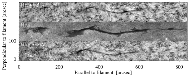
Figure 1: Slit-reconstructed image of the VTT observations with the Echelle spectrograph at different wavelength positions along the H$\alpha$ line. The giant filament extends over about 800″, displays a gap at the left hand side and an EFR appears as a bright area below the thin spine of the filament on the right-hand side. The observations were carried out on 2011 November 15 between 11:38 UT and 13:20 UT. From top to bottom: H$\alpha+0.5$ Å, H$\alpha$ line core, and H$\alpha-0.5$ Å. The white arrow points to disk center.

The main part of a filament is the spine. It appears as a dark elongated structure. The whole filament is a collection of thin threads, which are aligned with the magnetic field lines. Going out sideways from the spine we find the barbs, which are bundles of threads. They are magnetically linked to the photosphere (Engvold 2001; Lin et al. 2005). Through these barbs, mass can be transported into and out of the filament. The barbs and the spine, which contain the cool filament plasma, are defined with H$\alpha$ observations. In EUV observations the filament has a wider appearance (e.g., Aulanier & Schmieder 2002; Heinzel et al. 2003; Dudík et al. 2008). The filament contains mainly neutral hydrogen and helium as well as singly ionized helium. The EUV radiation, emitted by the quiet Sun, is absorbed by the Lyman H, He i, and He ii resonance continua. Anzer & Heinzel (2005) state that the neutral hydrogen absorbs EUV light below the hydrogen Lyman continuum at 912 Å. In addition, the authors describe that for lower wavelengths, absorption through neutral helium (below 504 Å) and singly ionized helium (below 228 Å) occurs. The dark absorption area is defined as the EUV filament channel. Dudík et al. (2008) found that the area covered by the EUV filament channel matches well with a magnetohydrostatic model of a linear filament flux tube. By co-aligning the central part of EUV and H$\alpha$ filaments, Aulanier & Schmieder (2002) deduce that the filament channel share some common properties in both wavelengths. Both are composed of the same magnetic dips, where plasma condensation appear. Furthermore, the authors show that the morphology of the filament is the same for observations in several wavelengths below 912 Å. Schmieder et al. (2008) conclude that the fine structure in 171 Å and H$\alpha$ filtergrams is similar because of the comparable optical thickness of H$\alpha$ and the He ii continuum.

Plasma is moving along the filament. Sometimes these horizontal flows move in opposite directions. Zirker et al. (1998) first described this bidirectional pattern of flows in a filament as “counter-streaming” flows based on H$\alpha$ observations. These flows are most clearly seen along threads of the filament’s spine, but can also occur in barbs (Zirker et al. 1998). Evidently, the formation of filaments is a continuous process, where mass is transported into and out of the filaments (Martin 2001). Counter-streaming flows are also reported in EUV observations, but compared to H$\alpha$ observations they often do not reach the combination of high spatial and temporal resolution (Labrosse et al. 2010). Alexander et al. (2013) found flows that are oppositely directed in adjacent threads in EUV data of the suborbital telescope High Resolution Coronal Imager (Hi-C, Cirtain et al. 2013; Kobayashi et al. 2014). They concluded that these flows are not visible in EUV images of the Atmospheric Imaging Assembly (AIA, Lemen et al. 2012) on board the Solar Dynamics Observatory (SDO, Pesnell et al. 2012) because of the low spatial resolution of AIA. In this study, we show that we are able to detect counter-streaming flows in AIA images by enhancing the image contrast (Sect. 4).

A giant quiet-Sun filament was present on the solar disk in November 2011. The main motivation of the present work is to analyze the dynamical aspects of this giant filament over a period of two hours. For this purpose we used space observations from AIA and the Helioseismic and Magnetic Imager (HMI, Schou et al. 2012) on board SDO, and H$\alpha$ observations of the Kanzelhöhe Solar Observatory (KSO) to define the spine of the filament. Furthermore, we demonstrate that it is possible to visualize counter-streaming flows in AIA images using an advanced image processing technique, i.e., noise adaptive fuzzy equalization (NAFE, Druckmüller 2013). The same filament was observed with the Echelle spectrograph of the Vacuum Tower Telescope (VTT, von der Lühe 1998) on Tenerife, Spain, on 2011 November 15 (Fig. 1). Kuckein et al. (2016) focused on the spectroscopic analysis of the filament. The authors found counter-streaming flows in the barbs of the filament, which they related to the mass supply of the filament.

In Sect. 2, we describe the observations and the image processing steps for SDO HMI, AIA, and KSO data. In Sects. 3 and 4, we present a description of the counter-streaming flows in the two-hour time series and use different methods to infer the horizontal proper motions along the filament’s spine. Furthermore, we focus on the visualization and detection of the counter-streaming flows in the spine of the filament using local correlation tracking (LCT, November & Simon 1988).

2 Observations

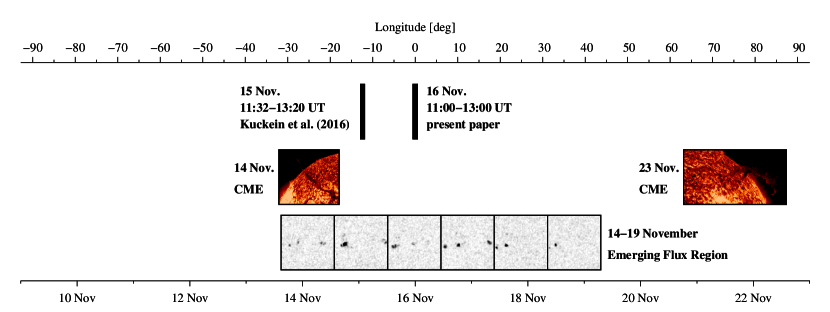
Figure 2: Timeline showing selected events related to the filament that occurred during the filament’s passage across the solar disk, also indicated in the lower axis showing the time of observations. The indicated dates refer to 12:00 UT. The longitudinal position of the middle of the filament is shown at the upper axis. The present observations were taken when the filament was centered on the central meridian. The timeline for the CMEs are shown from activation to eruption. The EFR, located to the right of the filament, is shown at different evolutionary stages.

2.1 Overview

On 2011 November 8 a giant filament appeared on the solar disk in the northern solar hemisphere. The eastern end of the filament erupted a few days later on November 14 as part of a coronal mass ejection (CME). On October 23 we were already able to recognize the filament in $\lambda$304 Å filtergrams of the Solar Terrestrial Relations Observatory (STEREO, Kaiser et al. 2008). In Fig. 1 we see the filament in H$\alpha$ as observed with the Echelle spectrograph of the VTT on November 15 (Kuckein et al. 2014, 2016). The H$\alpha$ line center image (middle row) shows that the filament has a gap on its left side caused by a CME a few hours before. In addition, an emerging flux region (EFR) at coordinates (740″, 10″) is visible as a bright plage in H$\alpha$ connected by some dark arch filaments just below the right end of the filament. In HMI continuum images, we see pores appearing between November 14 – 19 at the location of the EFR. By November 19 both EFR and pores have decayed. Furthermore, we observe many plage regions around the filament channel. Much of the filament erupted as a non-geoeffective CME on November 22, likely because of a nearby active region destabilizing the magnetic field topology. The filament vanished completely one day after the CME on November 23. An overview and timeline of the events around the filament is given in Fig. 2.

The observed giant filament does not fit into the category of polar-crown filaments because it covers several tens of degree in latitude and reaches into the sunspot latitude belt. Hence, we classify the filament into the wider category of quiet-Sun filaments. We examine a phenomenon, which has not been reported very often in the past, thus providing us the opportunity to compare its properties to regular-sized filaments.

2.2 SDO observations

On November 16 at around 12:00 UT the filament was centered on the central meridian (Fig. 2). Hence, we selected this time for further analysis. We used AIA and HMI data in order to investigate the spatial evolution of the giant filament. The study is based on AIA images taken in the EUV-wavelength bands centered at $\lambda$171 Å, $\lambda$193 Å, $\lambda$211 Å, and $\lambda$304 Å. The HMI instrument provides line-of-sight magnetograms and filtergrams of the continuum intensity. We selected observations of two hours from 11:00 – 13:00 UT with a cadence of 12 s for the AIA wavelength bands and 45 s for the HMI magnetograms and continuum images.

We downloaded Level 1.0 data, where the data had already gone through the basic reduction processes such as flat-field correction and conversion into FITS format (Lemen et al. 2012). With the help of a SSW routine, the different plate scales and roll angles of all four AIA telescopes were consolidated. The image scale was set to a value of 0$\aas@@fstack{\prime\prime}$6 pixel^-1 (DeRosa & Slater 2013) for both HMI and AIA images.

After data reduction, the images were prepared for the further analysis. The images have $4096\times 4096$ pixels containing the entire solar disk. For the purpose of limb-darkening subtraction from the HMI continuum images, we computed an average limb-darkening profile. We plotted the intensity values $I$ of each pixel as a function of $\mu=\cos\theta$, where $\mu$ is the cosine of the heliocentric angle $\theta$, and we fit it with a fourth-order polynomial:

$$I(\mu)=c_{0}+c_{1}\cdot\mu+c_{2}\cdot\mu^{2}+c_{3}\cdot\mu^{3}+c_{4}\cdot\mu^{4}.$$ (1)

This profile still includes dark sunspots and bright points in plage areas. To remove them from the profile a mask of these regions was created. The mask excluded these points, and the procedure was repeated but now with a first-order polynomial

$$I(\mu)=c_{0}+c_{1}\cdot\mu.$$ (2)

We expanded the one-dimensional limb-darkening profile to two dimensions and subtracted it from the HMI continuum images, which leads to a contrast enhancement and a flat background. Making the rough assumption that small-scale magnetic fields are perpendicular to the solar surface, the HMI magnetograms were divided by $\mu$, which carries out a coarse correction of geometric foreshortening to remove projection effects.

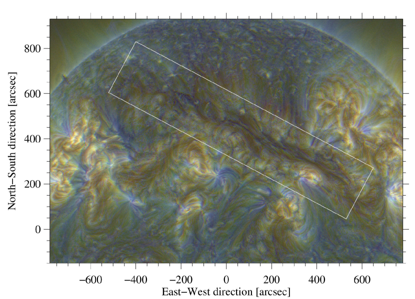
Figure 3: False-color image of the giant solar filament at 12:00 UT on November 16. The image is composed of three images obtained in the wavelength bands $\lambda$171 Å, $\lambda$193 Å, and $\lambda$211 Å. In the composed image different parts of the corona are highlighted. The blue parts show lower temperatures in the corona, while the yellow parts show the hotter regions. The filament appears as a dark structure enclosed by the white box crossing the Sun’s central meridian in the northern hemisphere.

Using AIA $\lambda$304 Å images, we selected a reference map at exactly the time when the center of the filament intersects the Sun’s central meridian, which occurs at 12:00 UT on November 16. To save memory and speed up processing we extracted a region of $2600\times 1800$ pixels in the northern hemisphere (Fig. 3). Routines in the SSW library facilitate a straightforward correction of the solar differential rotation. Thus, all data were properly aligned.

Because of the spherical shape of the Sun, we implemented geometric corrections to obtain a deprojected image of the filament in Cartesian coordinates and with square pixels. The origin of this coordinate system was placed at the lower left corner, and the values on the abscissa and ordinate are now given in megameters (see Fig. 4). For this purpose, we used a Delaunay triangulation (Lee & Schachter 1980). Here, irregularly gridded data were arranged in triangles by an algorithm. The surface values were then interpolated with another algorithm onto a regular grid using quadratic polynomial interpolation. This procedure is based on Verma & Denker (2011), who used it to correct Hinode G-band images (Kosugi et al. 2007). Furthermore, the filament is rotated $28$^∘ counterclockwise to have the filament axis horizontal for easier display (Fig. 4). The images are presented with the standard AIA color-coding. The images have a size of $3400\times 1200$ pixels, where one pixel represents an area of $320\,\mathrm{km}\times 320$ km on the solar surface. In Fig. 4b and c the EUV filament channel has a length of around 1000 Mm.

2.3 H$\alpha$ observations

We compare the EUV images of the filament with H$\alpha$ observations of the Kanzelhöhe Solar Observatory (KSO) at 12:00 UT on November 16 (Fig. 4a). The contrast of the KSO image was enhanced with a $\gamma$-correction. The KSO image was aligned with the SDO images and was geometrically corrected with the same procedure as for the AIA images. We extracted the contour of the H$\alpha$ filament to compare the appearance of the filament with the EUV observations. We see that the H$\alpha$ filament is much narrower than the EUV filament channel, as was reported in previous studies (e.g., Anzer & Heinzel 2005). In the H$\alpha$ image we recognize the spine of the filament and the barbs. Furthermore, we see the gap that was reported in the observations of Kuckein et al. (2016) for the previous day (Figs. 1 and 2). In the southeastern part of the filament we see further gaps in the spine. The EUV filament channel instead appears as a coherent structure where neither the gap nor the barbs are visible. The flows, which we describe in the following, are directly related to the cold filament material in the spine.

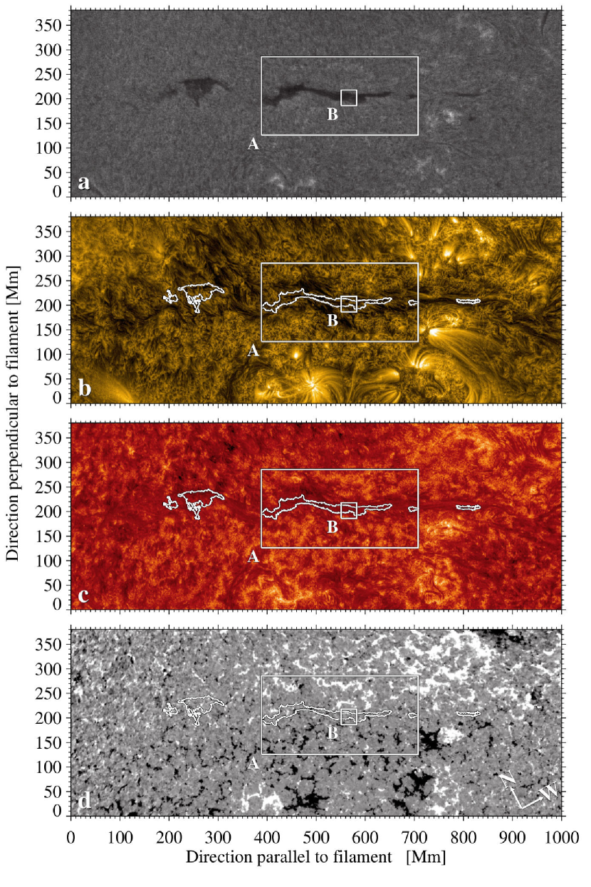
Figure 4: The filament at 12:00 UT on November 16. From top to bottom: (a) contrast enhanced H$\alpha$ image from Kanzelhöhe Solar Observatory, (b) contrast enhanced AIA $\lambda$171 Å image, (c) contrast enhanced AIA $\lambda$304 Å image, and (d) two-hour average of 160 magnetograms clipped between $\pm 25$ G. The contour of the H$\alpha$ filament in panel (a) is plotted in panels (b), (c), and (d). The white boxes labeled A and B mark the regions that we use later to determine the horizontal proper motions (region A, see Figs. 5 and 6) and the counter-streaming flows (region B, see Fig. 8)

3 Methods

To determine the horizontal proper motion along the filament, we use local correlation tracking (LCT, November & Simon 1988) applied to the AIA images. Furthermore, we use an advanced image processing tool to enhance the contrast in the AIA images, i.e., noise adaptive fuzzy equalization (NAFE, Druckmüller 2013).

3.1 Local correlation tracking

Horizontal proper motions play an important role in the dynamics of solar structures. A standard method used to measure horizontal velocity flows is LCT (e.g., November & Simon 1988; Verma & Denker 2011). In this method we determine displacement vectors from local cross-correlations between two images of a time series. We apply the LCT algorithm of Verma & Denker (2011) to the different AIA time series to measure the horizontal flow velocities along the spine of the filament.

First, we define a Gaussian kernel,

$$g(x^{\prime},y^{\prime})=\frac{1}{2\pi\sigma^{2}}e^{-\frac{r(x^{\prime},y^{\prime})^{2}}{2\sigma^{2}}},$$ (3)

for a high-pass filter, which is applied to suppress gradients related to structures larger than granules. The standard deviation,

$$\sigma=\frac{\mathrm{FWHM}}{2\sqrt{2\ln 2}},$$ (4)

is directly related to the full width at half maximum (FWHM), which has a value of 2000 km (6.5 pixels). We employ the LCT algorithm to sub-images $i(x^{\prime},y^{\prime})$ with a size of $16\times 16$ pixels, which refers to a size of $5120\,\mathrm{km}\times 5120\,\mathrm{km}$. Thus, the size of the final flow map will be reduced by the width of the sampling window. The coordinates $x^{\prime}$ and $y^{\prime}$ refer to the sub-image, where $r(x^{\prime},y^{\prime})=\sqrt{(x^{\prime 2}+y^{\prime 2})}$. The LCT algorithm is used on the whole time period of $\Delta T$ = 120 min, which contains 601 images with a time cadence of $\Delta t$ = 12 s. In the LCT algorithm we use a time cadence of $\Delta t^{\prime}$ = $8\times 12$ s = 96 s, in agreement with the results of Verma & Denker (2011).

3.2 Noise adaptive fuzzy equalization

The NAFE method is a qualitative method for processing solar EUV images of AIA to improve their contrast. In the following the mathematical method is presented as it is laid out in Druckmüller (2013). The NAFE method combines two classical methods, unsharp masking and adaptive histogram equalization, but does not suffer from their typical problems. By combining the two techniques, the resulting images are free of processing artifacts and the noise is well controlled and suppressed. The pixels of the original image $A$ depend linear on the intensity.

Applying NAFE to the original image $A$, the resulting image $B$ is then a linear combination of the images resulting from the gamma transformation $T_{\gamma}(A)$ and the NAFE transformed image $E_{N,\sigma}(A)$:

$$B=(1-w)\ T_{\gamma}(A)+wE_{N,\sigma}.$$ (5)

The parameter $w$ represents the weight of NAFE. By choosing the value $w=0$ the image passes only through the normal gamma transformation, which is a constant pixel value transform

$$T_{\gamma}(A)=b_{0}+(b_{0}+b_{1})\left(\frac{a_{1}-a_{0}}{A-a_{0}}\right)^{\gamma},$$ (6)

where $a_{0}$ and $a_{1}$ are constant input values, representing the zero emission intensity and the maximum value encountered in the data. The constants $b_{0}$ and $b_{1}$ are the minimum and maximum output values. Using lower values for $\gamma$ yields darker images, and higher values make the images brighter. In contrast to the gamma transform, the image in the NAFE method is passing through a pixel value transform, which varies for each pixel, also depending on its neighborhood (cf. Druckmüller 2013).

Druckmüller (2013) remarks that the NAFE method shows the best results for AIA $\lambda$171 Å images. Compared to other methods, this method adds no artifacts to the images and contrast and noise are well controlled. The only disadvantage is the long processing time when the method is applied to $4\mathrm{k}\times 4$k full-disk images.

The result after applying the NAFE method to the AIA $\lambda$171 Å images is shown in Fig. 4b. Values of $\gamma=2.6$ and $w=0.25$ for the NAFE parameters provide the best visual results. Evidently, the NAFE image shows a higher contrast. The structures in the images are sharper and richer in detail. Individual loops are clearly discernible in the EFR and other active regions, and single threads are uncovered along the filament’s spine.

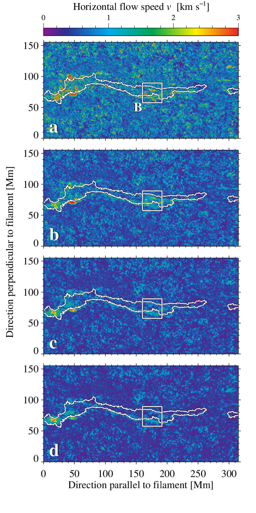
Figure 5: LCT flow speed maps of the spine of the filament (region A in Fig. 4). The LCT method was applied to the AIA $\lambda$171 Å time series for different time intervals $\Delta T$. The time intervals are (a) $\Delta T$ = 30 min, (b) $\Delta T$ = 60 min, (c) $\Delta T$ = 90 min, and (d) $\Delta T$ = 120 min. The square-region B shows the $32\,\mathrm{Mm}\times 32\,\mathrm{Mm}$ region of Fig. 8. The white contour outlines the filament as seen in H$\alpha$.

We also apply the NAFE method to the images in the AIA wavelength bands $\lambda$193 Å, $\lambda$211 Å, and $\lambda$304 Å (Figs. 3 and 4c, as well as Fig. 6 for all four wavelengths). For $\lambda$304 Å we used the input parameters of $\gamma=4.4$ and $w=0.25$. For $\lambda$193 Å and $\lambda$211 Å we used the pre-defined values of $\gamma$ and $w$ ($\lambda$193 Å: $\gamma=2.6$ and $w=0.20$; $\lambda$211 Å: $\gamma=2.7$ and $w=0.20$). In summary, for all these images we see an increase in the contrast of the images. We identify single threads in the spine and around the filament, and in the loop structure in the surrounding plasma.

4 Results

4.1 Horizontal flow fields in and around the filament

To track the horizontal flow fields in and around the filament we apply LCT to the contrast enhanced AIA $\lambda$171 Å images. The LCT map encompassing the whole EUV filament channel (Fig. 4) possesses a mean velocity of $\bar{v}=0.42$ km s^-1 with a standard deviation of $\sigma_{v}=0.25$ km s^-1, and a maximum velocity of $v_{\mathrm{max}}$ = 3.35 km s^-1. To inspect the LCT results more closely, we choose a ROI of $320\,\mathrm{Mm}\,\times\,160\,\mathrm{Mm}$ within the AIA $\lambda$171 Å images along the spine of the filament (region A in Fig. 4). First, we study how the time interval $\Delta T$ impacts the velocity. Hence, we run the LCT algorithm for the first 15 min, 30 min, 60 min, and 90 min of the time series, and for the whole time series of $\Delta T$ = 120 min.

In Fig. 5, we display the results for the time intervals $\Delta T$ = 30, 60, 90, and 120 min for LCT applied to region A in Fig. 4. In Table 1, the maximum and mean values as well as the standard deviation $\sigma_{v}$ for the velocities are listed. For the shorter time intervals the velocities are higher. The shorter the time interval, the closer is the flow speed related to the evolution of individual features. The highest velocities belong to the 15-minute time interval with a maximum velocity of $v_{\mathrm{max}}=7.7$ km s^-1. The smallest values for the maximum velocity $v_{\mathrm{max}}=3.3$ km s^-1 are found for the 90-minute time interval. The 120-minute time interval has a slightly higher maximum velocity of $v_{\mathrm{max}}=3.4$ km s^-1. In the 30-minute time interval small groups with high velocities are present in and around the spine (Fig. 5a). The longer the time interval, the smaller the number of regions with high velocities. In the 60- and 90-minute time interval, groups with high velocities are only located in the spine. However, in the longer time intervals the overall flow along the spine becomes visible (Fig. 5c and d) because the random velocity vectors are averaged and only persistent flows along the spine remain. The mean velocity shows the same tendency as the maximum velocity. It is highest in the shortest time interval with $\bar{v}=1.2$ km s^-1 and a standard deviation of $\sigma_{v}=0.8$ km s^-1. In the time interval of 120 min, the mean velocity is reduced to nearly one-third of the value in the shorter time interval, i.e., $\bar{v}=0.5$ km s^-1 and $\sigma_{v}=0.3$ km s^-1. Verma et al. (2013) presented in their study similar results by varying the time interval of LCT, where it was used on simulated granulation patterns. The averaged velocities from the 15- to 120-minute time intervals decreased by a factor of three (Fig. 3 in Verma et al. 2013). In our study LCT is applied to a small region of the filament’s spine in the corona (region A in Fig. 4). The averaged velocities for the different time intervals decreased by nearly 70% when the time intervals increase. We also recognize the absence of the extended flow features reported by Verma et al. (2013) in the 120-minute time interval compared to the 15-minute time interval.

Table 1: Comparison of the different horizontal velocities of the AIA $\lambda$171 Å flow maps for different time intervals $\Delta T$ of the LCT algorithm for region A of $315\,\mathrm{Mm}\times 155\,\mathrm{Mm}$ ($985\times 485$ pixels). We show the maximum velocities $v_{\mathrm{max}}$, as well as the mean velocities $\bar{v}$ with the corresponding standard deviation $\sigma_{v}$.

$\Delta T$	$v_{\mathrm{max}}$	$\bar{v}$	$\sigma_{v}$
[min]	[km s-1]	[km s-1]	[km s-1]
015	7.73	1.22	0.76
030	6.19	0.85	0.53
060	4.55	0.61	0.38
090	3.27	0.51	0.31
120	3.35	0.45	0.28

4.2 Counter-streaming flows

Counter-streaming flows have not yet been clearly seen in AIA EUV images. Alexander et al. (2013) compared Hi-C (Cirtain et al. 2013; Kobayashi et al. 2014) and AIA observations of a filament in the $\lambda$193 Å wavelength band. While the Hi-C data showed oppositely directed flows, even the enhanced AIA data did not reveal such flows. The authors attributed this discrepancy to the higher spatial resolution of Hi-C ($\sim$0$\aas@@fstack{\prime\prime}$3) compared to AIA ($\sim$1$\aas@@fstack{\prime\prime}$5, Lemen et al. 2012). This motivated us to study counter-streaming flows in our filament in more detail.

We create time-lapse movies for the two-hour time series of the high-cadence data set based on the original images and the contrast-enhanced images in the four AIA wavelength bands $\lambda$304 Å, $\lambda$171 Å, $\lambda$193 Å, and $\lambda$211 Å. In all image sequences we detect counter-streaming flows along the spine of the giant filament. For the ROI (Fig. 6 or region A in Fig. 4) we provide the time-lapse movies of the contrast-enhanced images for all four wavelengths as online material. The counter-streaming flows are present in all four wavelength bands in the same location of the spine. Especially at the beginning of the movie, we see a fast south-streaming flow in the upper half of the filament’s spine directed to the right and parallel to the filament. Parallel to it, slower flows in the same direction are observed (arrows in Fig. 6). Simultaneously, we see a north-streaming flow in the lower half of the filament’s spine directed to the left and also parallel to the filament. It appears that these counter-streaming flows are faster at the beginning of the time series and slow down towards the end. By the end of the time-lapse movie at around 12:45 UT the counter-streaming flows come to an end and are no longer clearly visible.

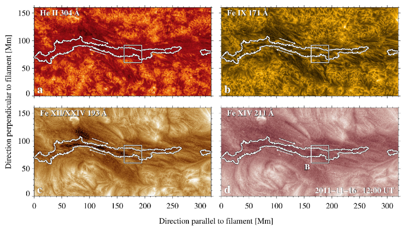
Figure 6: NAFE contrast enhanced images (region A with a size of $320\,\mathrm{Mm}\times 160\,\mathrm{Mm}$) of different AIA wavelengths at 12:00 UT on November 16: (a) $\lambda$304 Å, (b) $\lambda$171 Å, (c) $\lambda$193 Å, and (d) $\lambda$211 Å. We detect the counter-streaming flows in the time-lapse movies of the high-cadence data set (see online material)1. The white square (region B) outlines the $32\,\mathrm{Mm}\times 32\,\mathrm{Mm}$ region to which we apply LCT to track the counter-streaming flows (Fig. 8). The white arrows show location and direction of the counter-streaming flows along the spine. The white contour encloses the location of the filament’s spine in H$\alpha$.

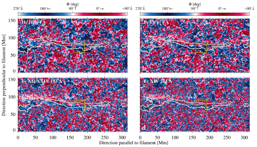
Figure 7: Illustration of counter-streaming flows based on the angle $\Phi=\mathrm{arccot}\ v_{x}/v_{y}$ for the different wavelengths: (a) $\lambda$304 Å, (b) $\lambda$171 Å, (c) $\lambda$193 Å, and (d) $\lambda$211 Å. Blue (red) indicates that the velocity vector is pointing to the left (right). The images were smoothed with a Lee filter. We show the contour of the H$\alpha$ filament in white. The yellow square shows a ROI of $32\,\mathrm{Mm}\,\times\,32\,\mathrm{Mm}$, where we applied LCT to track the counter-streaming flows (Fig. 8).

We use LCT to quantify counter-streaming flows for all four wavelengths. Therefore, we choose a ROI (Fig. 6), which has a size of $320\,\mathrm{Mm}\times 160\,\mathrm{Mm}$. For LCT we use the first 90 minutes of the two-hour time series because the counter-streaming flows are best seen here. The time-cadence of LCT is $\Delta t^{\prime}=96$ s. With this procedure we retrieve the horizontal velocities in the $x$- and $y$-directions, i.e., $v_{x}$ and $v_{y}$. To illustrate the counter-streaming flows in this region, we define the flow direction as the angle $\Phi$ between these two components

$$\cot\Phi=\frac{v_{x}}{v_{y}},$$ (7)

i.e., $\Phi=0\mbox{${}^{\circ}$}$ indicates flows directly to the right and $\Phi=180\mbox{${}^{\circ}$}$ to the left. Flows directly to the top and bottom are given by $\Phi=+90\mbox{${}^{\circ}$}$ and $-90\mbox{${}^{\circ}$}$, respectively. The directions of the horizontal velocity vectors are color-coded: the darkest red/blue is chosen for $\Phi=0\mbox{${}^{\circ}$}$/$180\mbox{${}^{\circ}$}$. In this way, the direction of flows predominantly along the filament’s spine are easily perceptible. The results for the four wavelengths are shown in Fig. 7. For the sake of clarity, the maps are gently smoothed with a Lee filter (Lee 1986) in order to emphasize the counter-streaming flows. In addition, we show the contour of the filament in H$\alpha$. The overall impression of each map is that the red color dominates, i.e., velocity vectors point to the right $\Phi\in(-90\mbox{${}^{\circ}$},\,+90\mbox{${}^{\circ}$})$. However, in the middle of each map, we see an elongated region between coordinates (50 Mm, 200 Mm) parallel to the filament axis and coordinates (65 Mm, 85 Mm) perpendicular to the filament axis, which only exhibits velocities directed to the left side of the image (blue). Directly above this blue region, we always have a homogeneous red area with velocities pointing to the right side. This shows the oppositely directed flows in this region of the filament and therefore provides evidence for counter-streaming flows. The contour of the filament in Fig. 7 shows that the counter-streaming flows are mainly located in the spine of the filament. This is best seen in AIA $\lambda$171 Å (Fig. 7b), but also in $\lambda$304 Å (Fig. 7a) and in $\lambda$193 Å (Fig. 7c). In $\lambda$211 Å (Fig. 7d) the region of counter-streaming flows is barely identifiable in the LCT maps. However, the $\lambda$211 Å movie shows a faint counter-streaming flow.

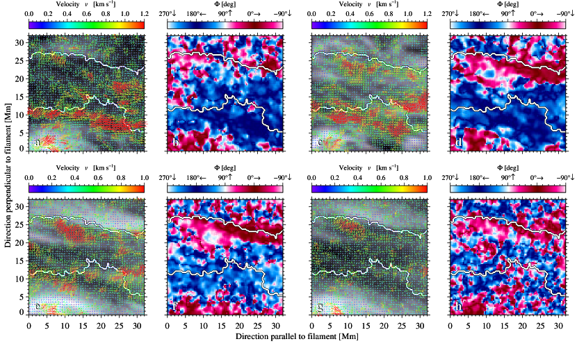
Figure 8: Validation of counter-streaming flows: (a, b) $\lambda$304 Å, (c, d) $\lambda$171 Å, (e, f) $\lambda$193 Å, and (g, h) $\lambda$211 Å. We show a region of $32\,\mathrm{Mm}\times 32\,\mathrm{Mm}$ (region B in Fig. 4). The left images (a, c, e, and g) show the summed image of each wavelength over the two-hour time series superposed with the horizontal velocity vectors derived with LCT. The right images (b, d, f, and h) display a map of the angle $\Phi$, which indicates the direction of the velocity vector (left is shown in blue and right in red). The white contour outlines the filament as seen in H$\alpha$.

To further validate the counter-streaming flows we pick out a small ROI of $32\,\mathrm{Mm}\times 32\,\mathrm{Mm}$ at the spine of the filament. This region is highlighted as a white and yellow square in Fig. 6 and 7, respectively. We show the averaged horizontal velocity vectors derived with LCT in Figs. 8a, c, e, and g. As the background, we show the average image of the two-hour time series. Next to each panel, we have the $\Phi$-map indicating the direction of the horizontal velocity vectors (Figs. 8b, d, f, and h). Figure 8 demonstrates that the counter-streaming flows are best seen in AIA $\lambda$171 Å (Fig. 8c). We detect in the lower half of the map flows pointing to the left (below 18 Mm on the $y$-axis). In the upper half of the image flows are directed to the right (above 19 Mm on the $y$-axis). This is clearly evident in the $\Phi$-map (Fig. 8d), where the lower half of the map is dominated by the color blue, while the upper half is dominated by the color red. The same pattern occurs in AIA $\lambda$193 Å for both the velocity vectors (Fig. 8e) and the flow direction map (Fig. 8f). The wavelength band $\lambda$304 Å shows a different pattern (Fig. 8a), where in the lower half of the image strong horizontal flows directed to the left still prevail, but in the upper half, the flows are directed to the top or only faint horizontal flows to the right are present. The dominance of the horizontal flows directed to the left is also visible in the $\Phi$-map (Fig. 8b), where the red parts in the upper half are not connected with each other. Both panels belonging to AIA $\lambda$304 Å (Figs. 8a and b) show no clear evidence for counter-streaming flows. Furthermore, we have inspected AIA $\lambda$211 Å images. In both panels of Figs. 8g and h, we see no clear indication of counter-streaming flows. We glimpse counter-streaming flows in the time-lapse movie; however, we cannot verify them with LCT. Most likely, the contrast in the $\lambda$211 Å images is not strong enough to yield a strong LCT signal, despite using NAFE on the images to enhance locally the image contrast.

Table 2: Averaged horizontal velocities for region B inside the H$\alpha$ contour of the filament’s spine separated in the velocities predominantly to the left (blue) and right (red) for all four wavelengths. We present the maximum horizontal velocities $v_{\mathrm{max}}$, the mean horizontal velocities $\bar{v}$, and the corresponding standard deviation $\sigma_{v}$.

$\lambda$	direction	$v_{\mathrm{max}}$	$\bar{v}$	$\sigma_{v}$	No. of
[Å]		[km s-1]	[km s-1]	[km s-1]	pixels
304	red	1.45	0.50	0.26	1268
	blue	2.29	0.70	0.37	3035
171	red	1.60	0.67	0.31	1686
	blue	2.51	0.71	0.40	2617
193	red	1.83	0.59	0.32	1950
	blue	1.47	0.56	0.28	2353
211	red	1.58	0.48	0.26	2087
	blue	1.42	0.47	0.24	2216

Applying LCT yields the horizontal velocities for the four EUV wavelengths of the small region B (Fig. 8). In the following we discuss the velocities inside the H$\alpha$ contours of the spine. We categorize the velocities into the two main directions: left (blue) and right (red), see Table 2 for all four wavelengths. For both AIA $\lambda$171 Å and $\lambda$304 Å the left-directed (blue) flows have higher mean and maximum values than the right-directed (red) flows. In addition, for both bands the mean left-directed velocity is virtually identical with $\bar{v}_{\mathrm{304\,\AA}}=0.70$ km s^-1 and $\bar{v}_{\mathrm{171\,\AA}}=0.71$ km s^-1. The maximum left-directed velocity for $\lambda$171 Å is higher than the maximum velocity for $\lambda$304 Å with $v_{\mathrm{max,\,304\,\AA}}=2.3$ km s^-1 and $v_{\mathrm{max,\,171\,\AA}}=2.5$ km s^-1. In comparison, the right-directed velocities (red) are lower by about 36% for both $\lambda$304 Å and $\lambda$171 Å. Figures 8a and c confirm the higher velocities to the left by inspecting the color-code and length of the horizontal velocity vectors. The number of pixels used in the averages are higher in the blue region with 3035 pixels in $\lambda$304 Å and with 2617 pixels in $\lambda$171 Å. The dominance of the blue part is also seen in Figs. 8b and d. For $\lambda$193 Å, where the counter-streaming flows are very prominent, the velocities for the left- and right-directed flows are very similar. However, the maximum horizontal velocity is somewhat higher in red, in contrast to $\lambda$171 Å and $\lambda$304 Å. The mean velocities are nearly the same for both directions in $\lambda$193 Å (Table 2). The number of pixels are also more balanced than for the other two wavelengths: 1950 pixels for red and 2353 pixels for blue. In $\lambda$211 Å we barely recognize counter-streaming flows in the LCT maps (Figs. 8g and h). The blue and red parts appear balanced, which is also reflected in the number of pixels for each direction with 2087 pixels and 2216 pixels for the red and blue part, respectively. Furthermore, the maximum and mean velocities are very similar, but lower than the other wavelength bands (Table 2). The red part has a slightly higher maximum horizontal velocity than the blue part, where the high velocities appear in a small area between coordinates (5 – 15 Mm, 20 – 27 Mm) in Fig. 8g.

5 Discussions

The giant filament was visible for more than two weeks and may have even existed longer before it rotated onto the visible part of the Sun. During the time of observations of the filament two non-geoeffective CMEs were released. The filament lifted off during the second CME.

We used LCT to determine the horizontal flow velocities. Applying this algorithm to the $\lambda$171 Å time series of the whole EUV filament channel provided a mean horizontal velocity of $\bar{v}_{\mathrm{LCT}}=0.42$ km s^-1 with a standard deviation $\sigma_{\mathrm{LCT}}=0.25$ km s^-1 and a maximum velocity of $v_{\mathrm{max}}=3.4$ km s^-1. Furthermore, we detected a strong dependency between the velocities and the length of the time intervals $\Delta T$ (Table 1): the longer the time interval, the lower the mean velocity value tracked with LCT. In general, the horizontal velocities tracked in a filament reach values of 5–30 km s^-1 (Labrosse et al. 2010). Comparing these values to our results, the average velocities we derived with LCT are much smaller. By averaging over a time series of two hours, we get the global flow field of persistent flows, and reduce the influence of evolving individual features (Verma et al. 2013). Nonetheless, in the shorter time intervals of 15 min or 30 min we reach maximum velocities of 6–8 km s^-1 in the spine of the filament. On the other hand, comparing our results with recent LCT studies by Verma & Denker (2012) on a decaying sunspot, our results are of the same order of magnitude.

Kuckein et al. (2016) observed the same giant quiet-Sun filament in the chromospheric H$\alpha$ line with the VTT on Tenerife. The authors concentrated on the analysis of the spectroscopic data. They derived average LOS velocities in the spine of $-0.29$ km s^-1 (upflows). Furthermore, they found signatures of counter-streaming flows in the barbs of the filament and proposed that the mass supply through the barbs is a good candidate to explain the supply with cold plasma in the filament. In the present study, we add to the previous results that counter-streaming flows are also present along the spine of this giant filament.

We compare the H$\alpha$ filament with observations in EUV. The EUV filament channel has a larger extension than the H$\alpha$ filament, as reported previously by, e.g., Dudík et al. (2008) and Aulanier & Schmieder (2002). In the latter study, the authors carefully analyzed the relations among filament channels seen in various transition-region and coronal lines. They conclude that all EUV filament channels observed with wavelengths lower than 912 Å show the same morphology. The authors mention that even for lower wavelengths of He ii 304 Å and Fe xii 195 Å their interpretation of filament channels is valid. Therefore, it is justified to assume that the observed plasma flows in the EUV channels are related to the H$\alpha$ filament.

Counter-streaming flows were observed in the visible and in the UV and EUV (for an overview see Labrosse et al. 2010). Most observations of counter-streaming flows are obtained in cool-plasma observations in H$\alpha$. Alexander et al. (2013) observed counter-streaming flows at subarcsecond scales along adjacent filament threads by direct imaging in the $\lambda$193 Å EUV wavelength band with high-resolution observations of an active region filament with Hi-C. The authors compared their results with AIA $\lambda$304 Å images and came to the conclusion that counter-streaming flows cannot be tracked in AIA images, due to the coarse image scale. Nevertheless, by applying an image enhancement technique (NAFE), we were able to clearly track counter-streaming flows along the spine of a giant filament with data from the SDO/AIA instrument in different wavelength bands. We examined time-lapse movies of the contrast-enhanced images in the four AIA wavelength bands $\lambda$171 Å, $\lambda$193 Å, $\lambda$211 Å, and $\lambda$304 Å and detected counter-streaming flows in all four wavelength bands along the spine of the filament. Even in the unprocessed images, under careful inspection, the counter-streaming flows are present, but at the visual detection limit. Hence, image enhancement techniques are crucial in order to detect this phenomenon, otherwise it might escape detection. Only with the processed images are we able to quantify the counter-streaming flows with LCT. We see differences in the morphology of the filament in the four EUV wavelength bands, which possibly can be explained by the different absorption characteristics of the EUV wavelength bands with respect to the hydrogen and helium continua.

A more detailed analysis was carried out by tracking counter-streaming flows using LCT on a smaller region in the middle of the spine (region A in Fig 4). We created a map of the dominant flow direction (Fig. 7). With this direction map, we identify regions that exhibit clear counter-streaming flows in the wavelength $\lambda$171 Å, $\lambda$193 Å, and $\lambda$304 Å. In $\lambda$211 Å, counter-streaming flows are also seen, but they are much weaker. To validate these results, we analyzed in detail an even smaller region (region B in Fig. 4). The $\lambda$171 Å and $\lambda$193 Å filtergrams show the most prominent counter-streaming flows. However, for $\lambda$304 Å we can only detect strong flows in one direction. For $\lambda$211 Å we detect a flow only to the right of the filament. We speculate that the reason for not detecting any counter-streaming flows in $\lambda$211 Å is the low contrast in the filtergrams, which complicates tracking with LCT.

Counter-streaming flows were first detected by Zirker et al. (1998) in the spine of a quiet-Sun filament by examining the blue and red wings of H$\alpha$ filtergrams. The opposite directed flows appear in different threads of the filament, not only in the spine but also in the barbs of the filament (as seen in the barbs of our filament by Kuckein et al. 2016). In conclusion, Zirker et al. (1998) propose that counter-streaming flows are common features in all quiet-Sun filaments. Counter-streaming flows are reported not only in quiet-Sun filaments, but also in active region filaments as reported by Alexander et al. (2013) and now also for extremely large filaments like the one presented in this work. Lin (2011) agrees with the statement that counter-streaming flows are common phenomena. Qiu et al. (1999) considers counter-streaming flows as a key feature to hold cool plasma stable inside filaments at coronal heights. These authors ascribe the counter-streaming motions to small-scale pressure imbalances that are located at the footpoints of the filament. These imbalances are caused by an unknown mechanism of the magnetic field. Inspecting the magnetograms, the overall magnetic configuration of the filament is stable. Lin et al. (2003) detect counter-streaming flows in H$\alpha$ filtergrams in the wings at $\pm 0.25$ Å and $\pm 0.45$ Å from line center along the spine of an polar crown filament and interprets them as evidence of a horizontal magnetic field parallel to the main body of the filament.

Chen et al. (2014) classified counter-streaming flows in two ways. The first class is ubiquitous small-scale counter-streaming flows, which are associated with longitudinal oscillations of single threads. The filament in the present study belongs to the second class and contains large-scale counter-streaming flows, which are limited to a certain area and are present in different threads. The area covers by visual inspection approximately 15–20% of the area of the entire filament. Inside this area, the counter-streaming flows were visible for at least two hours. The flows are persistent in time, but become less prominent at the end of the time series.

There are multiple studies reporting on the velocities in counter-streaming flows. Zirker et al. (1998) detected flow speeds in H$\alpha$ between 5–20 km s^-1. Lin et al. (2003) provided values of the same range with an average value of 8 km s^-1. Other studies have derived similar values of 5–15 km s^-1 (Yan et al. 2015; Schmieder et al. 2008, 2010) or 10–25 km s^-1 (Lin et al. 2008a, b; Shen et al. 2015). In EUV observations even higher velocities of up to 70 km s^-1 have been reported (Labrosse et al. 2010) where the authors point out a trend to higher velocities compared to H$\alpha$ observations. Furthermore, in the study of Alexander et al. (2013), who studied oppositely directed flows in EUV, velocities of 70–80 km s^-1 are tracked for an active-region filament along individual threads. Studies directly related to longitudinal oscillations showed slightly higher values of 10–40 km s^-1 (Li & Zhang 2012). Typically, counter-streaming flows were derived with time-slice diagrams (e.g., Lin et al. 2008b; Schmieder et al. 2010) or measuring of Doppler shifts (e.g., Lin et al. 2003; Schmieder et al. 2010). In the present study, we derived the horizontal flow speeds of the counter-streaming flows for the first time with LCT and obtained maximum values of 1.4–2.5 km s^-1, which are much lower than the reported values from other studies. The lower values can be explained by the chosen method, where the values are averaged over a time range of 90 min. Another parameter affecting LCT velocities is the size of the sampling window. If the choice of FWHM is either too small or too large, it will lead to the underestimation of the velocities (Verma et al. 2013) by mixing or averaging the flows in opposite directions. The FWHM we chose is around the size of a typical granule, which has been identified by Verma & Denker (2011) and Verma et al. (2013) as an optimal choice for tracking persistent horizontal proper motions in a time series.

Tracking single features manually in time-lapse movies revealed higher flow speeds of 20–30 km s^-1, but with relatively high measurement uncertainties of about 5 km s^-1. However, intensity variations do not necessarily imply plasma motions, thus the concept phase velocity more appropriately describes this phenomenon. Looking at a rapidly moving feature at the beginning of the time series, we derived a phase velocity higher than 100 km s^-1, but we cannot distinguish in the time-lapse movies whether this fast moving structure is directly related to the filament. In any case, the derived velocities of single features are comparable with results in the previous studies mentioned above.

Furthermore, we applied LCT to time series of KSO full-disk H$\alpha$ images. Because of the low spatial resolution and seeing affecting ground-based observations, we were not able to detect counter-streaming flows in the H$\alpha$ time-lapse movies or when applying LCT to these data.

6 Conclusions

We investigated the dynamics of the giant quiet-Sun filament over a time period of about two hours, which is a very narrow time range compared to the total lifetime of the filament (Fig. 2). To determine the proper motions of the cool filament’s plasma observed in different EUV wavelengths, we applied the LCT to the high-cadence SDO AIA time series. To increase the contrast in the AIA images we used the image enhancement technique NAFE, which provided detail-rich images with a high dynamic range. Thanks to this method it was possible to uncover counter-streaming flows along the filament and to quantify the velocities using the LCT method. By comparing the area with counter-streaming in EUV with H$\alpha$ data of KSO, we can conclude that the counter-streaming flows appear along the spine of the filament. We found counter-streaming flows in different wavelength bands. The counter-streaming flows are tracked most clearly in the wavelength bands $\lambda 171$ Å and $\lambda 193$ Å. Furthermore, the counter-streaming flows appear as persistent flows covering 15–20% of the filament’s area and are visible for at least two hours. They only become less prominent towards the end of the time series.

In order to analyze if counter-streaming flows are present in all quiet-Sun filaments, as stated by Zirker et al. (1998) and Lin et al. (2003), a larger statistic sample of quiet-Sun filaments including polar crown filaments could be used. Therefore, it is certainly beneficial to inspect the existing H$\alpha$ archives from, e.g., the Chromospheric Telescope (ChroTel, Kentischer et al. 2008; Bethge et al. 2011) and the Big Bear Solar Observatory (BBSO, Denker et al. 1999; Steinegger et al. 2000). In addition, similar studies to those presented in Kuckein et al. (2016) can be performed with the Echelle spectrograph at VTT in combination with Europe’s largest solar telescope GREGOR (Schmidt et al. 2012) to examine the fine structure of filaments in relation to the global size of filaments.