Towards platform-independent verification
of the standard mathematical functions:
the square root function

Abstract

The paper presents (human-oriented) specification and (pen-and-paper) verification of the square root function. The function implements Newton method and uses a look-up table for initial approximations. Specification is done in terms of total correctness assertions with use of precise arithmetic and the mathematical square root $\sqrt{\dots}$, algorithms are presented in pseudo-code with explicit distinction between precise and machine arithmetic, verification is done in Floyd-Hoare style and adjustment (matching) of runs of algorithms with precise arithmetics and with machine arithmetics. The primary purpose of the paper is to make explicit properties of the machine arithmetic that are sufficient to make verification presented in the paper. Computer-aided implementation and validation of the proofs (using some proof-assistant) is the topic for further studies.

Keywords: machine arithmetic, exact functions, formal verification, total and partial correctness, Floyd-Hoare method, square root, Newton method, look-up table, fix-point representation, floating-point representation

1 Introduction

1.1 Motivation

Let us start with a quotation from the abstract of the paper [18], because it correlates with the purpose of our paper very well:

Current critical systems commonly use a lot of floating-point computations, and thus the testing or static analysis of programs containing floating-point operators has become a priority. However, correctly defining the semantics of common implementations of floating-point is tricky, because semantics may change with many factors beyond source-code level, such as choices made by compilers.

The major difference between [18] and the present paper is the concern: the cited paper addresses problems with the floating-point value representation and arithmetics, while the present paper addresses the standard mathematical function platform-independent formal specification and formal verification by study in full details the square root function.

In our approach the platform-independence means that we specify properties of the functions and prove these properties for for approximate algorithms without building (some-how comprehensive) formal model of a particular processor architecture (like, for example, Intel’s processors in [8, 9, 11] or Oracle’s processors in [13]) or fix/floating-point formats (like, for example, in [2, 7, 18]) but carry out a proofs with several explicit simple assumptions how machine arithmetic relates to the precise arithmetic. Thus these explicit simple assumptions are sufficient conditions to validate on a particular processor with particular formats of numeric data in order to guarantee that a mathematical functions verified with these assumptions (square root function in this paper) meet their formal specification. We believe that our assumptions about machine arithmetic are valid for many platforms and are easy to check/validate.

Before we move to a literature survey on topics related to our study let us advocate importance of the formal verification of the software. Although our paper addresses verification in small (i.e. verification of small stay-alone programs), we would appeal in the next paragraph to importance of verification in large i.e. verification of complex cyber-physical systems. (Please refer slides 8-11 of [13] for justification of a need of verification in small, floating-point arithmetic, and the standard mathematical functions in particular.)

December 12, 2017, Roskosmos [28] has published the official results of investigation of the accident on November 28, 2017, which has led to loss of the Meteor-M satellite (altogether with another 18 satellites). Risks at start have been insured for the sum of 2,6 billion Russian rubles. Results of the investigation read [28] (translation by N.V. Shilov):

It has revealed the hidden problem in an algorithm which wasn’t shown for decades of successful launches of Sojuz carrier-rocket with the upper-stage accelerating block Fregate. … There was a combination of parameters of a launching-pad of the spaceport, azimuths of flight of the carrier-rocket and the accelerating block which hadn’t been met earlier. Respectively, it hasn’t been revealed at the carried-out on-land testing and simulation of a ballistic trajectory according to the standard adopted techniques.

The formal verification (in large as well as in small) is aimed to reveal “hidden problem in an algorithm which wasn’t shown for decades”, a rare “combination of parameters” that can’t be revealed “according to the standard adopted techniques”. We believe that a formal verification is a demand of the day and one of a few grad challenges for Computer Science research [12].

1.2 Literature survey

A need for better specification and validation of the standard functions is recognized (in principle) by industrial and academic professional community, as well as the problem of a conformance of their implementation with the specification. We would like to point out just on two papers [16, 17] that address formal complex specification and testing of standard mathematical functions. Hear we use adjunctive complex because these papers don’t restrict function properties by accuracy but take into consideration, for example, that $\sin$ and $\cos$ are odd and even functions respectively, they match pythagorean normalization equality $\sin^{2}x+\cos^{2}x=1$ for all real $x\in\mathbb{R}$. An educational value and issues of better documentation and specification of the standard functions are discussed in papers [22, 23].

Several studies have been published on platform-dependant formal verification of mathematical functions, including division [4, 9], square root [20, 9, 21, 4], trigonometric [8], exponential [10], and gamma [24] functions. Also several studies have been published on axiomatization of machine arithmetic (mostly binary floating-point arithmetic for the IEEE-754 standard [26]) to prove basic mathematical properties and consequently prove correctness of mathematical functions [2, 7, 3, 1].

First let us remark that even platform-independent verification of the integer square root function is not a trivial exercise. Please refer, for example, paper [21] where some standard mathematical integer functions (including the square root) are specified and verified in PVS.

Paper [2] formalizes machine arithmetic using Z-notation and present an implementation of the specification written in Occam. It presents a formal description of several mathematical functions over floating-point numbers, namely: rounding, addition, multiplication, square root, type-casting to integer, comparisons, etc. Besides it, the paper specifies five classes of floating-point numbers: NaN, Inf, zero, normal and denormal numbers. Then four modes of rounding and error conditions are presented. The implementation includes representations of floating-point numbers, its rounding and packing/unpacking and basic finite mathematical procedures. The main algorithm pattern for a binary operation with floating-point values (according to [2]) is as follows:

1. unpack both operands into their sign, exponent and mantissa fields;

2. denormalise both by shifting in the leading bit of the mantissa if necessary;

3. perform the operation with denormalized arguments;

4. pack the result and then round the packed result.

Next paper [7] presents an approach to verification in HOL Light of several floating-point operations of a new (at time of publication) Intel computer architecture IA-64:

Correctness of the mathematical software starts from the assumption that the underlying hardware floating point operations behave according to the IEEE standard 754 for binary floating point arithmetic. Actually, IEEE-754 doesn’t explicitly address floating-point machine arithmetic operations, and it leaves underspecified certain significant questions, e.g. NaN propagation and underflow detection. Thus, we not only need to specify the key IEEE concepts but also some details specific to IA-64.

This paper starts with a theory of floating point arithmetic, which is non specific to any format and afterwards specifies IA-64 formats in details. Floating-point numbers in [7] are presented in highly generic way (as $\pm k\times 2^{E-N}$) but have a canonical representation and normalized form. The paper argues also that the concept of the unit in the last place (ulp) has several different definitions but all have some counterintuitive properties; due to this reason the paper adopts a modified definition from [19]. Four types of rounding (to-Nearest, Down, Up, to-Zero) are defined in [7]; in contrast to the IEEE standard rounding is defined for numbers with an unbounded exponent range, but all overflows are handled during operations execution.

Paper [3] describes syntax and semantics of floating-point arithmetic theory. Besides being general, the formalization seriously rely upon Satisfiability Modulo Theories (SMT) approach. The paper has 2 certain contributions: mathematical structures for floating-point model, a signature for a theory of floating-point arithmetic and an interpretation of its operators in terms of the mathematical structures defined earlier. Thus, it is designed to be a formal reference for automatic theorem provers providing built-in support for reasoning about floating-point arithmetic.

It is important to prove correctness of mathematical functions widely used in different architectures and libraries. The square root function is required (by IEEE-754) to be exact (please refer the next section 2 for the definition). Hence, correctness of this function (as well as other exact functions) should be considered with a special attention.

Approach to verification of the square root function suggested in paper [4] is based on a concept of a digit serial method (DSM) for a number: DSM for a real number $x\in\mathbb{R}$ is an algorithm that determines the digits of $x$ serially, starting with the leading digit. The main contribution of the paper is a generic DSM analysis method for determining bounds on the magnitudes of the digits, as well as bounds on the error associated with the estimates. (We believe that the approach may be related to interval techniques [14].)

In the papers [5, 20] authors prove correctness of the square root algorithm used in Power4 processor. The algorithm uses Chebyshev polynomials. Despite of the fact that the algorithm has more steps comparing to the Newton (also known as Newton-Raphson) method used in [11], only one iteration is enough to get necessary accuracy; also, because less instructions are reliant on the earlier ones in the polynomial algorithm, the algorithm is better for parallelization. The verification in [5, 20] is divided by two parts: proof of Taylor’s theorem and proof of properties of the square root function using Taylor’s theorem. One of the biggest challenges in the study in [20] was to approximate error size of Chebyshev polynomial with Taylor’s series as the former has a better approximation. To escape this problem hundreds of Taylor’s series were evaluated. The proof has been carried-out using non-standard analysis book (library) in ACL2.

1.3 Paper structure

In the next section 2 we present specification of the square root function according to the C programming language standard, sketch Newton method to compute approximations for the square root, formalize it as $SQR$ algorithm (with until-loop) and specify it in Floyd-Hoare style by a total correctness assertion [6] assuming the precise arithmetic (i.e. for mathematical reals).

In section 3 we give a pen-and-paper verification of the algorithm $SQR$ from the previous section 2 using Floyd-Hoare approach [6] and assuming the precise arithmetic: partial correctness is considered in the subsection 3.1 and termination — in the subsection 3.2.

Section 4 presents two modifications of the square root algorithm $SQR$: the first algorithm $ISQR$ differs from $SQR$ by use of an auxiliary function to “compute” good initial approximations (see subsection 4.1), the second algorithm $FSQR$ (see subsection 4.2) is a for-loop-based algorithm that uses the same auxiliary function but (in contrast to $ISQR$) estimates the number of sufficient iterations to achieve the required accuracy of the approximations. Both algorithms in this section are specified and verified under assumption that the arithmetic is precise.

The following-up section 5 starts with the subsection 5.1 where we formulate assumptions about fix-point values and arithmetic, and then presents and specifies the fix-point algorithm $fixSQR$ in the subsection 5.2.

The algorithm $fixSQR$ is verified (manually) in the section 6 by comparison with runs of algorithm $FSQR$ on the same input data. In the same section 5 we specialise the algorithm $fixSQR$ into better algorithm $mixSQR$ which is correct because of correctness of the algorithm $fixSQR$.

Section 7 presents our assumptions about floating-point arithmetic, the algorithm $fltSQR$ that computes approximations for the square root function in floating-point arithmetic, its specification and pen-and-paper verification. The algorithm is based on square root extraction from mantissa (using the fix-point algorithm $mixSQR$) and integer division to compute the exponent.

In the last section 8 we summarise the content and contribution of the present paper and discuss the topics for further research.

2 What is the standard function sqrt?

The C reference portal at en.cppreference.com/w/c specifics the the square root function sqrt [25] as it represented in the Appendix 0.A. It is easy to see an ambiguity in the specification: it first says that sqrt(2) must be $\sqrt{2}$, but then (in the Notes) that the error of sqrt(2) must be less than $0.5$ of ulp — the unit in the least precision (that is type and platform dependable. Of course, we have to rule out the first option (that sqrt() is $\sqrt{\ }$) as non-realistic; instead we have and examine in details the second one.

The standards mentioned in the specification are IEEE 754-2008 Standard for Floating-Point Arithmetic and the international standard ISO/IEC 60559:2011 [27] (that is identical to IEEE 754-2008). Section 9 of the standard recommends fifty operations that language standards should define (but all these operations are optional, not required in order to conform the standard). Some of these operations (including sqrt() as a special case of the function $(\ )^{1/n}$ for $n=2$), if being implemented, must be (according to the standard’ terminology) exact i.e. to round correctly (i.e. with an error less than $0.5$ulp). Due to this use of the term exact for computer functions and operation, let us fix another term precise when we speak about mathematical functions and operations with mathematical real numbers $\mathbb{R}$.

The first problem with the standard is type and platform dependence of the concept of the exact function: the accuracy upper bound $0.5$ulp depends on numeric type (float vs. double) as well as on implementation of the types (i.e. memory size reserved for the types). Another very critical problem with the specification and ISO/IEC/IEEE standards above is the absence (in the specification and standards) of a description of any validation procedure to check/prove that an implementation conforms the specification/standard.

Instead of requiring that sqrt computes the exact values for square roots in type- and/or platform-dependent way, it makes sense to specify another “standard” generic function (say $SQR(\ ,\ )$) for generic numeric data types with two parameters: the first parameter is for passing the argument value $Y\geq 0$ and the second — for passing the accuracy value $Eps>0$; the function is for computing $\sqrt{Y}$ with the accuracy $Eps$.

The accuracy of this function $SQR$ (i.e. the most wanted property and the only property specified in the standard) can be formally specified by any (or both) of the following two assertions:

• for all type-legal values $y\geq 0$ and $\varepsilon>0$, $SQR(y,\varepsilon)$ differs from $\sqrt{y}$ by no more than $\varepsilon$, i.e. $|\sqrt{y}-SQR(y,\varepsilon)|\leq\varepsilon$;

• for all type-legal values $y\geq 0$ and $\varepsilon>0$, $\big{(}SQR(y,\varepsilon)\big{)}^{2}$ differs from $y$ by no more than $\varepsilon$, i.e. $\big{|}y-(SQR(y,\varepsilon)\big{)}^{2}\big{|}\leq\varepsilon$.

It makes sense to fix the first formal specification for better compatibility with the concept of the exact standard function, since in this case we can define the standard function sqrt via SQR as follows:

    float sqrt(float Y)
    {return((float)SQR(Y, default(float)/2.0);}

where default is another new type- and platform-dependent feature (similar to sizeof) that returns the value of the unit in the least precision for a numeric type.

One may select any reasonable and feasible computation method to approximate $\sqrt{\ }$. For example, it can be a very intuitive, easy-to-implement and popular in education (e.g. [19, 15]) Newton Method:

1. input the number (to compute the square root) and guess an initial approximation for the root;

2. compute the arithmetic mean between the guess and the number divided by the guess; let this mean be a new guess;

3. repeat step 2 while the difference between the new and the previous guesses isn’t small enough (i.e. doesn’t feet the use-defined accuracy).

(Please refer to Fig. 1 for a sample implementation of the function for the data type float.)

float ab(float X)
{if (X<0) return(-X); else return(X);}

float SQR(float Y, float Eps)
{float X, D;
       X=Y;
       do {D=(Y/X-X)/2; X+=D;} while (ab(D)>=Eps/2);
return X;}

Figure 1: A floating-point function to compute a square root approximation

Both floating-point functions in Fig. 1 are easy to specify formally in a Hoare style [6]:

$$\left\{\begin{array}[]{l}[X\ is\ float]\ ab(X)\ [returned\ value\ =|X|],\\ [Y\geq 0\ and\ Eps>0\ are\ floats]\\ \hskip 28.45274ptSQR(Y,\ Eps)[|returned\ value\ -\sqrt{Y}|\leq Eps].\end{array}\right.$$ (1)

(Remark that the specification is incomplete since it doesn’t specify the program behavior and output if input values are $Y<0$ and/or $Eps\leq 0$.)

For a generic square root function with a generic numeric data type for input and output values, the specification (1) should be modified:

$$\begin{array}[]{c}[TYPY\ is\ a\ numeric\ type,\ Y\geq 0:\ TYPE,\ and\ Eps>0:\ TYPE]\\ SQR(Y,\ Eps)\ [|returned\ value\ -\sqrt{Y}|\leq Eps].\end{array}$$ (2)

If these specifications are proved, then SQR may be a good alternative to the standard function sqrt.

Unfortunately, it is not easy to prove these specifications automatically and formally because of several reasons. The major one is a problem that we already discussed in the literature survey in the introduction section 1 — an axiomatization of the computer-dependent floating-point arithmetic. Even a manual pen-and-paper verification of the algorithm $SQR$ (assuming precise arithmetic for real numbers $\mathbb{R}$) is not a trivial exercise that we solve in the next section.

3 Pen-and-paper verification of $SQR$

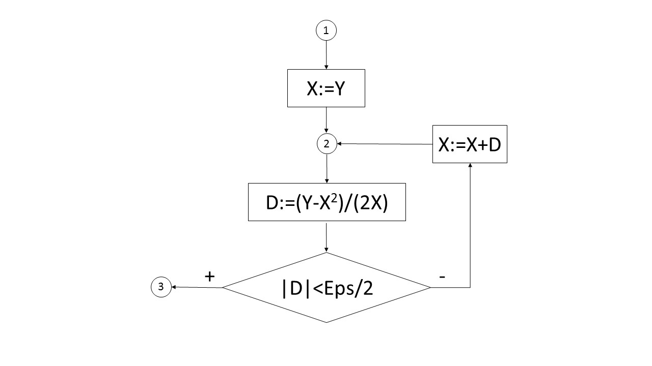
Figure 2: A flowchart of the algorithm $SQR$

Fig. 2 shows a flowchart of the algorithm (a little bit modified) of the function from Fig. 1. Let us refer to the algorithm as $SQR$ in the sequel. Having specified the algorithm in the same way as the function, we need to prove the following “relaxation” of the second triple in (2):

$$[Y,Eps\in\mathbb{R}\ \&\ Y\geq 0\ \&\ Eps>0]\ SQR\ [|X-\sqrt{Y}|\leq Eps]$$ (3)

To prove this assertion, let us consider three disjoint cases for the range of the initial value of the variable $Y$: $0\leq Y<1$, $Y=1$ and $Y>1$:

$$[Y,E\in\mathbb{R}\ \&\ 0\leq Y<1\ \&\ Eps>0]\ SQR\ [|X-\sqrt{Y}|\leq Eps],$$ (4)

$$[Y,E\in\mathbb{R}\ \&\ Y=1\ \&\ Eps>0]\ SQR\ [|X-\sqrt{Y}|\leq Eps],$$ (5)

$$[Y,E\in\mathbb{R}\ \&\ Y>1\ \&\ Eps>0]\ SQR\ [|X-\sqrt{Y}|\leq Eps].$$ (6)

The second case (5) is trivial. Two other cases (4) and (6) are “ideologically” very similar, so we prove below in this section the assertion (6) only. Due to this reason we assume below in the subsections 3.1 and 3.2 that the initial (input) variable values meet the precondition $Y,E\in\mathbb{R}\ \&\ Y>1\ \&\ Eps>0$ and that all operation used in the algorithm are precise mathematical operations with reals.

3.1 Partial Correctness

Let us employ the Floyd method [6] for a pen-and-paper proof of partial correctness. Let us select the control points 1, 2, and 3 as depicted in Fig. 2 to cut the flowchart into three loop-free paths:

path (1..2)

from the starting point 1 to point 2;

path (2+3)

from point 2 to the final point 3 via the positive branch;

path (2–2)

from point 2 to the same point 2 via the negative branch.

Let us consider all these paths one by one using the following annotations for the control points:

1. $Y>1\ \&\ Eps>0$ (i.e. the pre-condition);

2. $Y>1\ \&\ Eps>0\ \&\ \sqrt{Y}\leq X\leq Y$ (the loop invariant);

3. $|X-\sqrt{Y}|\leq Eps$ (i.e. the post-condition).

The first path (1..2) is easy to verify:

$$\frac{(Y>1\ \&\ Eps>0)\rightarrow(Y>1\ \&\ Eps>0\ \&\ \sqrt{Y}\leq Y\leq Y)}{\{Y>1\ \&\ Eps>0\}\ X:=Y\ \{Y>1\ \&\ Eps>0\ \&\ \sqrt{Y}\leq X\leq Y\}}.$$

The second path (2+3) is not so easy. Let us introduce a test program construct $\phi?$ as a short-hand for $if\ \phi\ then\ stop\ else\ abort$. Then verification of the path (after some simplification) is as follows:

$$\begin{array}[]{c}(Y>1\ \&\ Eps>0\ \&\ \sqrt{Y}\leq X\leq Y\ \&\ |\frac{Y-X^{2}}{2X}|<Eps/2)\ \rightarrow\ |X-\sqrt{Y}|<Eps\\ \\ \hline\cr\\ \{Y>1\ \&\ Eps>0\ \&\ \sqrt{Y}\leq X\leq Y\}\ D:=\frac{Y-X^{2}}{2X}\ \{|D|<Eps/2\ \rightarrow\ |X-\sqrt{Y}|<Eps/2\}\\ \\ \hline\cr\\ \{Y>1\ \&\ Eps>0\ \&\ \sqrt{Y}\leq X\leq Y\}\ D:=\frac{Y-X^{2}}{2X}\ ;\ |D|<Eps/2?\ \{|X-\sqrt{Y}|<Eps\}\end{array}$$ (7)

The premise

$$(Y>1\ \&\ Eps>0\ \&\ \sqrt{Y}\leq X\leq Y\ \&\ |\frac{Y-X^{2}}{2X}|<Eps/2)\ \rightarrow\ |X-\sqrt{Y}|<Eps$$

is valid since in this case we have

$$|X-\sqrt{Y}|=\Big{(}\frac{|X-\sqrt{Y}|\ (X+\sqrt{Y})}{2X}\Big{)}\times\Big{(}\frac{2X}{X+\sqrt{Y}}\Big{)}\leq\frac{Eps}{2}\times\frac{2}{1+\frac{\sqrt{Y}}{X}}<Eps.$$

The proof (also after some simplification) of the third path (2–2) is as follows:

$$\begin{array}[]{c}\\ (Y>1\ \&\ Eps>0\ \&\ \sqrt{Y}\leq X\leq Y\ \&\ |\frac{Y-X^{2}}{2X}|\geq Eps/2)\ \rightarrow\\ \rightarrow\ (Y>1\ \&\ Eps>0\ \&\ \sqrt{Y}\leq\frac{Y+X^{2}}{2X}\leq Y)\\ \\ \hline\cr\\ \\ \{Y>1\ \&\ Eps>0\ \&\ \sqrt{Y}\leq X\leq Y\}\\ D:=\frac{Y-X^{2}}{2X}\\ \{|D|\geq Eps/2\ \rightarrow\ (Y>1\ \&\ Eps>0\ \&\ \sqrt{Y}\leq X+D\leq Y)\}\\ \\ \hline\cr\\ \\ \{Y>1\ \&\ Eps>0\ \&\ \sqrt{Y}\leq X\leq Y\}\\ D:=\frac{Y-X^{2}}{2X}\ ;|D|\geq Eps/2?\ ;\ X:=X+D\\ \{Y>1\ \&\ Eps>0\ \&\ \sqrt{Y}\leq X\leq Y\}\end{array}$$ (8)

A hint to prove the premise of this derivation:

• $(Y>1\ \&\ \sqrt{Y}\leq X)\ \rightarrow\ (Y>1\ \&\ \sqrt{Y}\leq\frac{Y+X^{2}}{2X})$
  since $(Y>1\ \&\ \sqrt{Y}\leq X)$ implies $X>1$ and, hence, both sides of the AM-GM inequality $X\sqrt{Y}\leq\frac{Y+X^{2}}{2}$ may be divided by $X$;

• $(Y>1\ \&\ \sqrt{Y}\leq X\leq Y)\ \rightarrow\ (Y>1\ \&\ \frac{Y+X^{2}}{2X}<Y)$
  since $(Y>1\ \&\ \sqrt{Y}\leq X\leq Y)$ implies $\frac{Y-X^{2}}{2X}\leq 0$ and, hence, $\frac{Y+X^{2}}{2X}\ =\ X+\frac{Y-X^{2}}{2X}\leq\ Y+\frac{Y-X^{2}}{2X}\ \leq\ Y$.

3.2 Termination

Let us prove below that the loop invariant $Y>1\ \&\ Eps>0\ \&\ \sqrt{Y}\leq X\leq Y$ implies that every loop iteration reduces the absolute value of $D$ twice at least.

For it let us fix some $y>1$ as the initial value of the variable $Y$, $\varepsilon>0$ as the initial value of the variable $Eps$, let $x_{1}$, $x_{2}$, $\dots$ $x_{n}$, $x_{(n+1)}$, $\dots$ be the values of the variable $X$ immediately before $1^{st}$, $2^{nd}$, $\dots$ $n$-th, $(n+1)$-th, etc., iteration of the loop for this fixed initial value $y$ of $Y$, and let $d_{1}$, $d_{2}$, $\dots$ $d_{n}$, $d_{(n+1)}$, $\dots$ be the values of the variable $D$ immediately after $1^{st}$, $2^{nd}$, $\dots$ $n$-th, $(n+1)$-th, etc., iteration of the loop (also for the same fixed initial value $y$ of $Y$). In particular, $x_{1}=y$ and $d_{n}=\frac{y-x_{n}^{2}}{2x_{n}}$, $x_{(n+1)}=x_{n}+d_{n}$ for all $n>0$.

Let us express $d_{(n+1)}$ in terms of $d_{n}$:

$d_{(n+1)}=\frac{y-x_{(n+1)}^{2}}{2x_{(n+1)}}=\frac{y-(x_{n}+d_{n})^{2}}{2(x_{n}+d_{n})}=\frac{y-(\frac{y+x_{n}^{2}}{2x_{n}})^{2}}{2\frac{y+x_{n}^{2}}{2x_{n}}}=$

$=-\frac{(y-x_{n}^{2})^{2}x_{n}}{4x_{n}^{2}(y+x_{n}^{2})}=-\frac{d_{n}^{2}x_{n}}{y+x_{n}^{2}}=-\frac{d_{n}^{2}}{2x_{(n+1)}}$.

Note that all values $d_{1}$, $d_{2}$, $\dots$ $d_{n}$, $d_{(n+1)}$, $\dots$ are negative due to the loop invariant. Hence

$$\frac{|d_{(n+1)}|}{|d_{n}|}=\frac{d_{(n+1)}}{d_{n}}=-\frac{d_{n}}{2x_{(n+1)}}=\frac{1}{2}\times\frac{x_{n}^{2}-y}{x_{n}^{2}+y}<\frac{1}{2}.$$

It implies $|d_{(n+1)}|<\frac{y-\sqrt{y}}{2^{n}}$, i.e. the algorithm terminates after at most

$$1+\log_{2}\frac{y-\sqrt{y}}{\varepsilon}$$

iterations of the loop.

4 Towards machine-oriented square root algorithm

4.1 Improved square root algorithms based on until-loop

In spite being very efficient (due to a logarithmic complexity) the algorithm may be improved (optimized). Firstly, since we study case when $1<Y$ and know (from the loop invariant) that $\sqrt{Y}\leq X\leq Y$, it makes sense to compute directly the absolute value $AD:=\frac{X^{2}-Y}{2X}$ of $D$ instead of computing $D:=\frac{Y-X^{2}}{2X}$ and then $|D|$ in the loop condition. Next, we may use a fast hash function $SUP:(1,\infty)\rightarrow(1,\infty)$ to compute good initial upper approximations instead of a very rough initial upper approximation used in the algorithm $SQR$. (For example, it may be rounded-up square roots.) While the first optimization just saves on each loop iteration on calls of the function computing the absolute value, the second one reduces the number of loop iterations. Fig. 3 shows a flowchart of the improved algorithm that we refer as the algorithm $ISQR$ in the sequel.

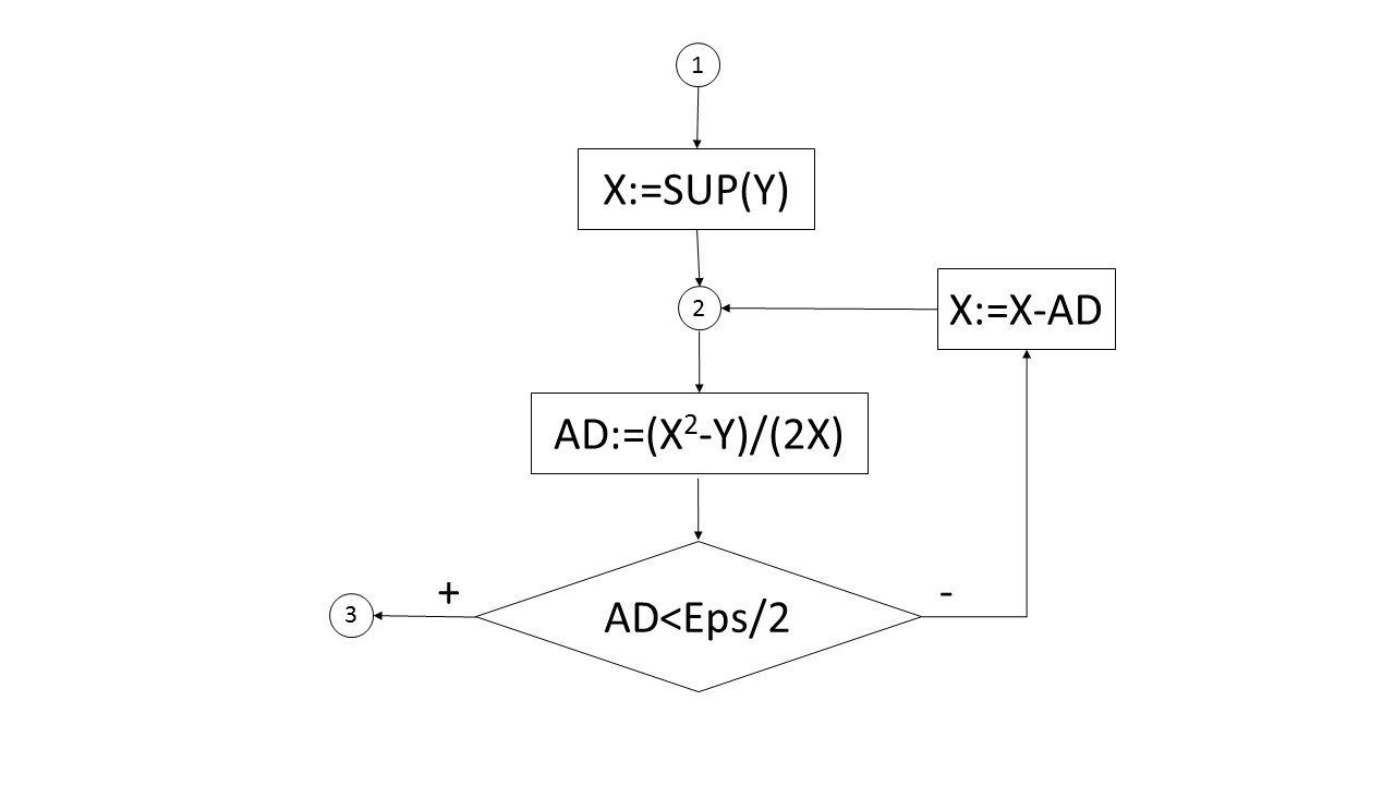
Figure 3: A flowchart of the improved (optimized) algorithm $ISQR$

For example if the function $SUP$ returns the rounded-up square roots, $y>1$ is the initial (input) value of the variable $Y$, and $\varepsilon>0$ is the initial (input) value of variable $Eps$ (accuracy) then $0\leq SUP(y)-\sqrt{y}<1$ and, hence, an upper bound for the number of the loop iterations in the algorithm $ISQR$ is

$$1-\log_{2}\varepsilon\ \geq\ 1+\log_{2}\frac{SUP(y)-\sqrt{y}}{\varepsilon}$$

instead of an upper bound

$$1+\log_{2}y-\log_{2}\varepsilon\ \geq\ 1+\log_{2}\frac{y-\sqrt{y}}{\varepsilon}$$

for the number of the loop iterations in the non-optimized algorithm $SQR$.

To prove the following total correctness assertion

$[Y>1\ \&\ Eps>0\ \&\ \forall y\in(1,+\infty):\sqrt{y}\leq SUP(y)\leq y)]$

$ISQR\ [|X-\sqrt{Y}|<Eps]$

we need to prove the partial correctness only since the termination are proved already by providing an upper bound for the number of the loop iterations.

For proving the partial correctness we may use the same control points 1, 2, and 3 to cut the flowchart into three loop-free paths (1..2), (2+3), (2–2), and the same annotations for the control points 2 (the loop invariant) and 3 (the post-condition) as for the algorithm $SQR$, but need to extend the precondition ($Y>1\ \&\ Eps>0$) of the $SQR$ by specification of the function $SUP$:

$$\forall y\in(1,+\infty):\sqrt{y}\leq SUP(y)\leq y.$$

The above proof (7) of the path (2+3) and the proof (8) of the path (2–2) remains valid. The first path (1..2) is easy to verify:

$$\begin{array}[]{c}\\ (Y>1\ \&\ Eps>0\ \&\ \forall y\in(1,+\infty):\sqrt{y}\leq SUP(y)\leq y)\ \rightarrow\\ \rightarrow\ (Y>1\ \&\ Eps>0\ \&\ \sqrt{Y}\leq SUP(Y)\leq Y)\\ \\ \hline\cr\\ \{Y>1\ \&\ Eps>0\ \&\ \forall y\in(1,+\infty):\sqrt{y}\leq SUP(y)\leq y)\}\\ X:=SUP(Y)\ \{Y>1\ \&\ Eps>0\ \&\ \sqrt{Y}\leq X\leq Y\}\end{array}$$ (9)

4.2 For-loop-based square root algorithms
(when more means better)

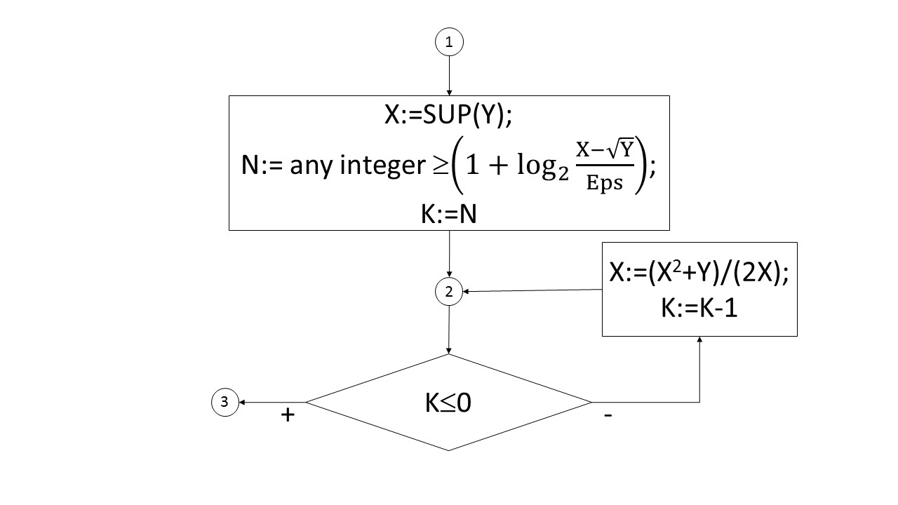
Figure 4: A flowchart of the non-adaptive for-loop-based algorithm $FSQR$

As we already proved, for every initial value $y>1$ of the variable $Y$ and every initial value $\varepsilon>0$ of the variable $Eps$ termination of the improved square root algorithm is guaranteed after (at most) $1+\lceil\log_{2}\frac{SUP(y)-\sqrt{y}}{\varepsilon}\rceil$ loop iterations, where $\lceil\dots\rceil$ is integer round-up function. Hence is possible to compute approximations for the square root by a non-adaptive for-loop-based algorithm $FSQR$ which flowchart depicted in Fig. 4. The algorithm uses a non-deterministic assignment

$$N:=\mbox{ any integer }\geq\big{(}1+\log_{2}\frac{X-\sqrt{Y}}{Eps}\big{)}$$ (10)

(where $\lceil\dots\rceil$ stays for integer rounding up). The corresponding correctness assertion is

$$\begin{array}[]{c}[Y>1\ \&\ Eps>0\ \&\ \forall y\in(1,+\infty):\sqrt{y}\leq SUP(y)\leq y)]\\ FSQR\ [|X-\sqrt{Y}|<\frac{Eps}{2}].\end{array}$$ (11)

Termination of the algorithm $FSQR$ is guaranteed by design since it is for-loop-based. Informally speaking the partial correctness of the algorithm follows from the partial correctness of the algorithm $ISQR$: while $\frac{X^{2}-Y}{2X}\geq Eps$ values of $X$ in both algorithms are equal in each iteration, and then $FSQR$ exercises several more iterations that move value of $X$ closer to $\sqrt{Y}$. Nevertheless we would like to make this argument more formal and in Floyd-Hoare style [6].

Let us select the control points 1, 2, and 3 as depicted in Fig. 4 and annotate them as follows:

1. $Y>1\ \&\ Eps>0\ \&\ \forall y\in(1,+\infty):\sqrt{y}\leq SUP(y)\leq y)$;

2. $Y>1\ \&\ Eps>0\ \&\ \sqrt{Y}\leq X\leq Y\ \&\ N\geq 1+\log_{2}\frac{SUP(Y)-\sqrt{Y}}{Eps}\ \&$
   $\&\ 0\leq K\leq N\ \&\ X-\sqrt{Y}\leq\frac{SUP(Y)-\sqrt{Y}}{2^{N-K}}$;

3. $|X-\sqrt{Y}|\leq\frac{Eps}{2}$ (i.e. the post-condition).

Proof of the path (1..2) is trivial since at the end of this path $N\geq 1+\lceil\log_{2}\frac{SUP(Y)-\sqrt{Y}}{Eps}\rceil$, $N-K=0$ and $X=SUP(Y)$.

Proof of the path (2–2) just follows the proof of the similar path for the algorithm $SQR$ with the following addendum: $0\leq K\leq N$ before the loop implies $0\leq K\leq N$ after the loop because of the loop condition $K>0$ that holds on this path before the assignment $K:=K-1$.

Proof of the path (2+3) is more complicated: at the end of the path

1. $K=0$ (due to the invariant at start of the path and the loop condition);

2. $\sqrt{Y}\leq X$ (due to the invariant at start of the path);

3. according to (2) $|X-\sqrt{(}Y)|=X-\sqrt{Y}$;

4. according to (1), (3) and the invariant $|X-\sqrt{(}Y)|\leq\frac{SUP(Y)-\sqrt{Y}}{2^{N}}$;

5. $\frac{SUP(Y)-\sqrt{Y}}{2^{N}}\leq\frac{SUP(Y)-\sqrt{Y}}{2^{1+\log_{2}\frac{SUP(Y)-\sqrt{Y}}{Eps}}}=\frac{SUP(Y)-\sqrt{Y}}{2\times\frac{SUP(Y)-\sqrt{Y}}{Eps}}=\frac{Eps}{2}$
   (because $N\geq 1+\log_{2}\frac{SUP(Y)-\sqrt{Y}}{Eps}$);

6. according to (4) and (5) $|X-\sqrt{Y}|\leq\frac{Eps}{2}$.

We have proved a stronger assertion for $FSQR$ than for $SQR$ and $ISQR$. Moreover, the proof implies that more iterations means better accuracy of computations (in the precise arithmetic, of course).

5 Square root algorithm for fix-point arithmetics

5.1 Fix-point machine arithmetics

One of the problems with the improved and for-loop-based algorithms is how to implement an efficient function $SUP$. A hint is use of a numeric data type $T$ with a (huge maybe) finite set of values $Val_{T}\subset\mathbb{R}$ instead of an infinite set $\mathbb{R}$. Then the function $SUP$ may be implemented in two steps:

• define an efficient rounding up function $round:Val_{T}\rightarrow Val_{T}$,

• pre-compute and memorize a look-up table $root$ with good upper approximations for the roots for each of the rounded values.

Further details and steps depend on selected numeric data type. In this and the next sections we study fix-point numeric data and algorithms with fix-point arithmetic. (We study of $floating-point$ data and algorithms later in the section 7.)

We understand fix-point numeric data type $T$ as follows:

• the set of values $Val_{T}$ is a finite subset of mathematical reals $\mathbb{R}$ such that

  • it comprises all reals in some finite range $[-\inf_{T},\sup_{T}]$, where $\inf_{T}>2$, $\sup_{T}>2$, with some fixed step $\frac{1}{2}>\delta_{T}>0$,

  • and includes all integer numbers $Int_{T}$ in this range $[-\inf_{T},\sup_{T}]$;

• legal binary arithmetic operations are

  • addition and subtraction; if not the range overflow exception then these operations are precise: they equal to the standard mathematical operations assuming their mathematical results fall in the range $[-\inf_{T},\sup_{T}]$ (and due to this reason are denoted as $+$ and $-$);

  • multiplication $\otimes$ and division $\oslash$; these operations are approximate but correctly rounded in the following sense: for all $x,y\in Val_{T}$

    • if $x\times y\in Val_{T}$ then $x\otimes y=x\times y$;

    • if $x/y\in Val_{T}$ then $x\oslash y=x/y$;

    • if $x\times y\in[-\inf_{T},\sup_{T}]$ then $|x\otimes y-x\times y|<\delta_{T}/2$;

    • if $x/y\in[-\inf_{T},\sup_{T}]$ then $|x\oslash y-x/y|<\delta_{T}/2$.

• legal binary relations are equality and all standard inequalities; these relations are precise, i.e. they equal to the standard mathematical relations (and due to this reason are denoted as $=$, $\neq$, $\leq$, $\geq$, $<$, $>$).

Due to the assumptions about the set of values

$$Val_{T}=\{n\times\delta_{T}\ :\ n\in\mathbb{Z}\mbox{ and }-\mbox{inf}_{T}\leq n\times\delta_{T}\leq\mbox{sup}_{T}\};$$

according the assumptions about integer values $Int_{T}$ within the range of $Val_{T}$

$$[-2..2]\subseteq Val_{T}\mbox{ and }\frac{1}{\delta}_{T}\in\mathbb{N}.$$

In case when multiplication is guaranteed to be precise (the mathematical product is in $Val_{T}$) then let us use the standard notation $\times$ instead of $\otimes$; similarly in case when division is guaranteed to be precise (the mathematical dividend is in $Val_{T}$) then let us use the standard notation $/$ instead of $\oslash$.

5.2 Fix-point variant of the square root: algorithm and specification

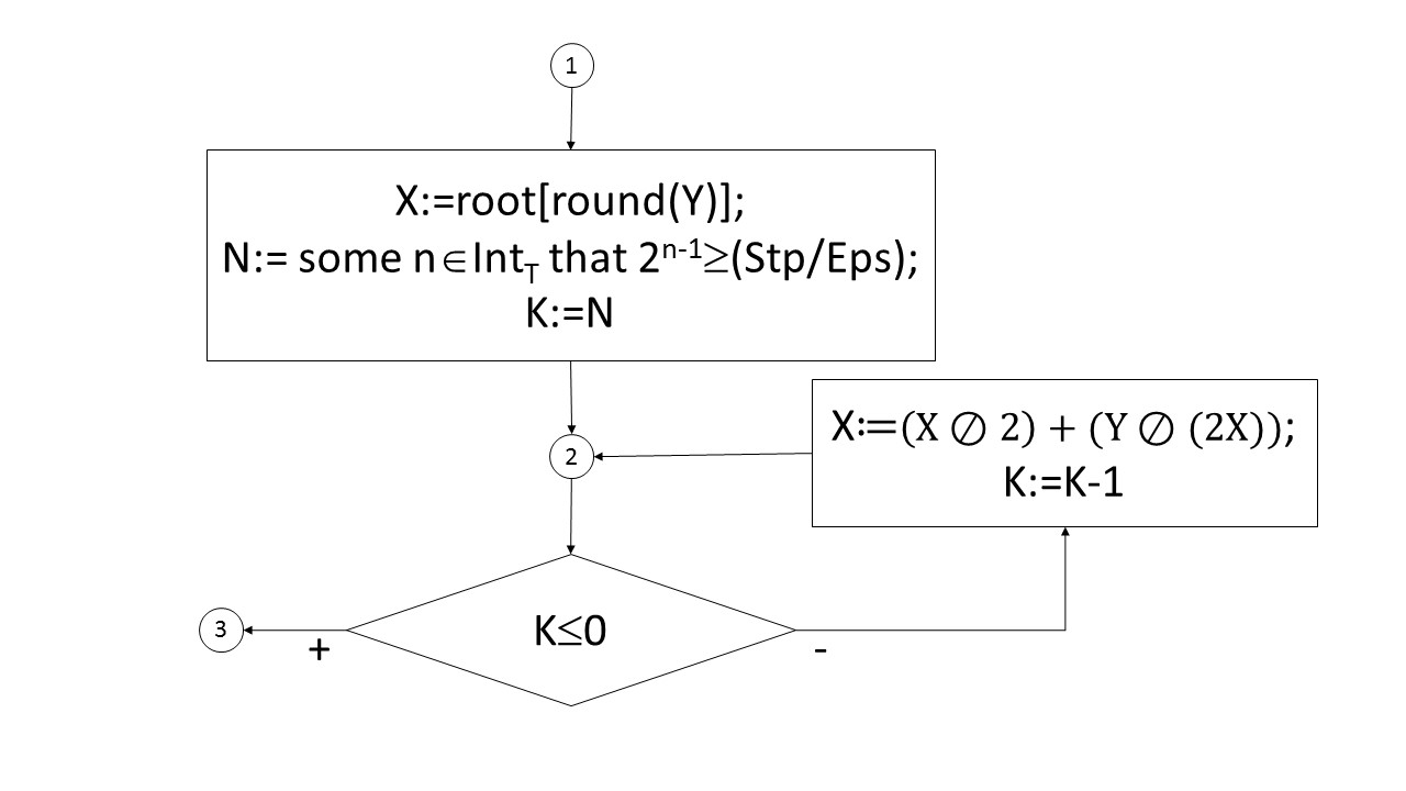
Figure 5: A flowchart of the square root algorithm $fixSQR$ for fix-point arithmetic

A non-adaptive algorithm $FSQR$ (Fig. 4) that uses mathematical operations transforms into algorithm $fixSQR$ (Fig. 5) that uses machine fix-point operations. This algorithm also (as $FSQR$) uses a non-deterministic assignment operator

$$N:=\mbox{ some }n\in Int_{T}\mbox{ that }2^{n-1}\geq\frac{Stp}{Eps}$$ (12)

that differs from the assignment (10) by use of some instead of any: this difference means that later we select the value instead of use an arbitrary one.

In the new algorithm we use an additional variable $Stp$ for a positive value in $Val_{T}$, an array $root$, and a function $round$ that have the following properties:

STEP:

value of $Stp$ is a multiple of the accuracy $Eps$, divides $\sup_{T}$ and is used to define the set $Arg_{Stp}=\{n\times Stp\ :\ n\in\mathbb{N}\mbox{, and }1<n\times stp\leq\sup_{T}\}$;

ROOT:

$root$ is a pre-computed look-up table indexed by $Arg_{Stp}$ such that $root[v]-\delta_{T}<\sqrt{v}\leq root[v]$ for each index $v\in Arg_{Stp}$;

ROUND:

the function $round:Val_{T}\rightarrow Arg_{Stp}$ is a rounding-up such that $round(u)-step<u\leq round(u)$ for each $u\in Val_{T}$, $u>1$.

Comment on the STEP property: we consider as a very natural the assumption that

• $Stp$ is a multiple of the accuracy $Eps$ since in the “limit” case $Eps=\delta_{T}$ and this $Eps$ divides any $Stp\in Val_{T}$;

• $Stp$ divides the “extreme” value $\sup_{T}$ because this value should be provided with a pre-computed square root upper approximation.

We are ready to specify correctness of the square root algorithm $fixSQR$ with fix-point arithmetic:

$$\begin{array}[]{c}[Y\in Val_{T}\ \&\ Y>1\ \&\ Eps\in Val_{T}\ \&\ Eps>0\ \&\\ \&\ \mathbf{STEP}\ \&\ \mathbf{ROOT}\ \&\ \mathbf{ROUND}]\\ fixSQR\ [|X-\sqrt{Y}|<\big{(}\frac{Eps}{2}\ +\ N\times\delta_{T}\big{)}].\end{array}$$ (13)

6 Pen-and-paper verification of $fixSQR$
(more may be worse)

Termination of the algorithm $fixSQR$ is straightforward since it is a for-loop-based algorithm. So we need to prove partial correctness only. We do this proof below by adjustment (or comparison) of runs of algorithm $fixSQR$ with fix-point arithmetics and algorithm $FSQR$ with precise arithmetics.

Let us select and fix hereafter initial values $x$, $y$, $s$, $\varepsilon$ for the variables $X$, $Y$, $Stp$, and $Eps$, and a look-up table $root$ and a function $round$ such that meet the precondition in (13). Let $SUP:(1,\infty)\rightarrow(1,\infty)$ be the function defined as follows:

$$SUP(u)=\left\{\begin{array}[]{l}root[v]\mbox{, if }u\in(1,\mbox{sup}_{T}]\mbox{, }v\in Arg_{Stp}\mbox{ and }u\in(v-s,v]\mbox{;}\\ u\mbox{ otherwise.}\end{array}\right.$$

Then this function and the initial values of $X$, $Y$, and $Eps$ meet the precondition in (11).

Let $nn$ be a particular value assigned to $N$ by the non-deterministic assignment operator (12) in the algorithm $fixSQR$. Remark that $SUP(y)-\sqrt{y}\leq s$ due to the following arguments:

$$\big{(}SUP(y)\big{)}^{2}\leq y+s\leq y+2s\sqrt{y}+s^{2}=(\sqrt{y}+s)^{2};$$

hence this value $nn$ is also a legal value of the non-deterministic expression

$$\mbox{ any integer }\geq\big{(}1+\log_{2}\frac{SUP(y)-\sqrt{y}}{\varepsilon}\big{)}$$

that is the right-hand expression in the assignment (10). It implies that both algorithms $FSQR$ and $fixSQR$ have legal runs with the initial values $x$, $y$, $\varepsilon$ for the variables $X$, $Y$, and $Eps$ where both have exactly $nn$ iterations of their loops.

Let $x^{\prime}_{0}$, $\dots$ $x^{\prime}_{nn}$ and $x^{\prime\prime}_{0}$, $\dots$ $x^{\prime\prime}_{nn}$ values of the variable $X$ in these runs after $0$-iterations, $\dots$ $nn$-iterations of the corresponding loop. (In particular, $x=x^{\prime}_{0}=x^{\prime\prime}_{0}$ is the initial value of $X$ and $x^{\prime}_{nn}$ and $x^{\prime\prime}_{nn}$ are the final values of the variable upon termination.)

Let us prove by induction on $k\in[0..nn]$ that

$$|x^{\prime}_{k}-x^{\prime\prime}_{k}|\leq k\delta_{T}.$$ (14)

Basis:

$x=x^{\prime}_{0}=x^{\prime\prime}_{0}$.

Assumption:

$|x^{\prime}_{k}-x^{\prime\prime}_{k}|\leq k\delta_{T}$ for all $k\in[0..n]$, where $n<nn$.

Step:

Let $\Delta=x^{\prime}_{n}-x^{\prime\prime}_{n}$; ($|\Delta|\leq n\delta_{T}$ due to the assumption.)

1. $x^{\prime}_{n+1}=\frac{x^{\prime}_{n}}{2}+\frac{y}{2x^{\prime}_{n}}$;

2. $x^{\prime\prime}_{n+1}=x^{\prime\prime}_{n}\oslash 2+y\oslash(2x^{\prime\prime}_{n})=\big{(}\frac{x^{\prime\prime}_{n}}{2}+\delta_{a}\big{)}+\big{(}\frac{y}{2x^{\prime\prime}_{n}}+\delta_{b}\big{)}$ where $|\delta_{a}|,|\delta_{b}|\leq\frac{\delta_{T}}{2}$;

3. $|x^{\prime\prime}_{n+1}-x^{\prime}_{n+1}|=|\frac{x^{\prime\prime}_{n}-x^{\prime}_{n}}{2}+\frac{y}{2}\big{(}\frac{1}{x^{\prime\prime}_{n}}-\frac{1}{x^{\prime}_{n}}\big{)}+(\delta_{a}+\delta_{b})|\leq$
   $\leq\frac{|x^{\prime\prime}_{n}-x^{\prime}_{n}|}{2}+\frac{y}{2}\big{|}\frac{1}{x^{\prime\prime}_{n}}-\frac{1}{x^{\prime}_{n}}\big{|}+|\delta_{a}+\delta_{b}|\leq\frac{|\Delta|}{2}+\frac{y}{2}\big{|}\frac{1}{x^{\prime\prime}_{n}}-\frac{1}{x^{\prime}_{n}}\big{|}+\delta_{T}$;

4. (Taylor’ expansion) $\frac{1}{x^{\prime\prime}_{n}}=\frac{1}{x^{\prime}_{n}+\Delta}=\frac{1}{x^{\prime}_{n}}-\frac{\Delta}{(x^{\prime}_{n})^{2}}+\theta$,
   where $\theta$ is a converging alternating series, $|\theta-\frac{\Delta}{(x^{\prime}_{n})^{2}}|\leq|\frac{\Delta}{(x^{\prime}_{n})^{2}}|$;

5. (from 4) $\frac{y}{2}\big{|}\frac{1}{x^{\prime\prime}_{n}}-\frac{1}{x^{\prime}_{n}}\big{|}=\frac{y}{2}\big{|}\theta-\frac{\Delta}{(x^{\prime}_{n})^{2}}\big{|}\leq\frac{y}{2}\times\frac{|\Delta|}{(x^{\prime}_{n})^{2}}\leq\frac{y}{2}\times\frac{|\Delta|}{y}=\frac{|\Delta|}{2}$;

6. (from 3 and 5) $|x^{\prime\prime}_{n+1}-x^{\prime}_{n+1}|\leq\frac{|\Delta|}{2}+\frac{y}{2}\big{|}\frac{1}{x^{\prime\prime}_{n}}-\frac{1}{x^{\prime}_{n}}\big{|}+\delta_{T}\leq\frac{|\Delta|}{2}+\frac{|\Delta|}{2}+\delta_{T}$;

7. (from 6) $|x^{\prime\prime}_{n+1}-x^{\prime}_{n+1}|\leq|\Delta|+\delta_{T}\leq n\delta_{T}+\delta_{T}=(n+1)\delta_{T}$.

According to the the proven total correctness assertion (11) $|x^{\prime}_{nn}-\sqrt{y}|\leq\frac{\varepsilon}{2}$; together with the proven property (14) it implies $|x^{\prime\prime}_{nn}-\sqrt{y}|\leq\big{(}\frac{\varepsilon}{2}+nn\times\delta\big{)}$; since $x^{\prime\prime}_{nn}$ and $nn$ are the values of the variables $X$ and $N$ in the algorithm $fixSQR$, it finishes the proof of the assertion (13).

One can remark that correctness of the assertion (13) implies that more iterations of the loop may be worse in accuracy (due to the addend $N\times\delta_{T}$ in the postcondition).

Our proof of the assertion (13) implies correctness of the following assertion

$$\begin{array}[]{c}[Y\in Val_{T}\ \&\ Y>1\ \&\ Eps\in Val_{T}\ \&\ Eps>0\ \&\\ \&\ EPS\geq 2\delta_{T}(2+\log_{2}\frac{Stp}{Eps})\ \&\\ \&\ \mathbf{STEP}\ \&\ \mathbf{ROOT}\ \&\ \mathbf{ROUND}]\\ mixSQR\ [|X-\sqrt{Y}|<Eps].\end{array}$$ (15)

where $mixSQR$ is algorithm depicted on Fig. 6.

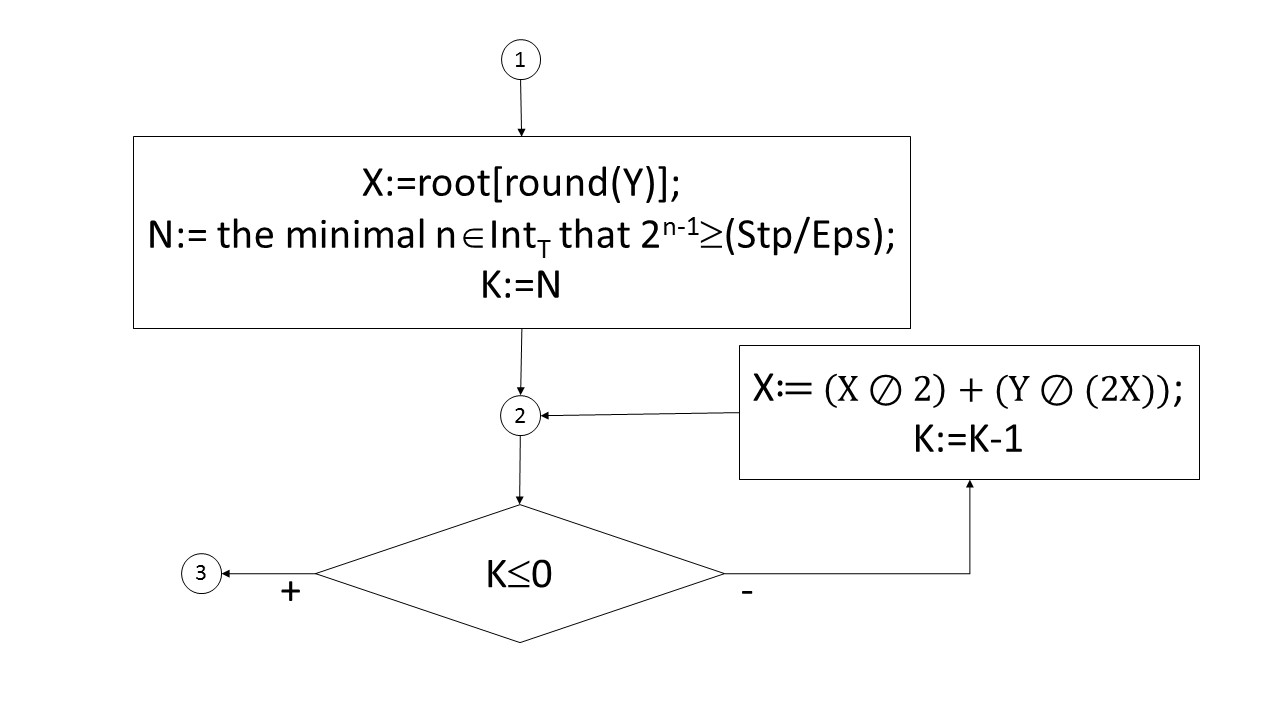
Figure 6: A flowchart of the square root algorithm $mixSQR$ for fix-point arithmetic

The assertion is valid due to the arguments represented in the next paragraph.

The algorithm $mixSQR$ is a specialization of the algorithm $fixSQR$ with deterministic assignment

$$N:=\mbox{ the minimal }n\in Int_{T}\mbox{ that }2^{n-1}\geq\frac{Stp}{Eps}$$

instead of the nondeterministic assignment (12). The precondition in (15) expands the precondition in (13) by the addend $EPS\geq 2\delta_{T}(2+\log_{2}\frac{Stp}{Eps})$ that means that the interval $[(1+\log_{2}\frac{Stp}{Eps}),\frac{Eps}{2\delta_{T}}]$ has length $\geq 1$, i.e. contains an integer. Let $y$, $\varepsilon$, $s$ be initial values of $Y$, $Eps$, and $Stp$ that satisfy the precondition in (15) (and hence the precondition in (13)), and let $nn$ be the minimal $n\in Int_{T}$ that $2^{n-1}\geq\frac{Stp}{Eps}$ (i.e. the value assigned to the variable $N$). Since $y$, $\varepsilon$, $s$ satisfy the precondition in (13), the algorithm $mixSQR$ stops on these initial data with final values of the variables that satisfy the postcondition in (13), i.e. $|x^{\prime}-\sqrt{y}|<\big{(}\frac{\varepsilon}{2}\ +\ nn\times\delta_{T}\big{)}$, where $x^{\prime}$ is the final value of $X$; since the value of $N$ is $nn$ then $nn\times\delta_{T}<\frac{\varepsilon}{2\delta_{T}}\times\delta_{T}=\frac{\varepsilon}{2}$; put it altogether we get that $|x^{\prime}-\sqrt{y}|<\varepsilon$, i.e. the postcondition in (15) is true.

7 Square root algorithm for floating-point arithmetic

In contrast to the fix-point numeric data type in the subsection 5.1, we aren’t going to specify properties of floating-point arithmetic operations (since we don’t need them to compute square root function) but just the properties of the set of floating-point values and couple of type-casting operations (that convert floating-point values into fix-point values and back).

Let $T$ be a fix-point numeric data type that satisfies the properties specified in the subsection 5.1. We understand floating-point numeric data type $F$ as follows:

• the set of values $Val_{F}$ is a finite subset of mathematical reals $\mathbb{R}$ that comprises some reals in some finite range $[-\inf_{F},\sup_{F}]$, where $\inf_{F},\sup_{F}>2$ and $\{0,\inf_{F},\sup_{F}\}\subseteq Val_{F}$;

• there are two unary operations $Man:Val_{F}\rightarrow Val_{T}$ (called mantissa), $Exp:Val_{F}\rightarrow Int_{T}$ (called exponent), and an integer constant $\beta_{T}\in Int_{F}$ (called exponent base or just base) such that for all positive $x\in Val_{F}$

  • $1<Man(x)<\frac{sup_{T}}{\beta_{F}}$;

  • if $inf_{T}$ is odd then $-inf_{T}<Exp(x)$ else $-inf_{T}\leq Exp(x)$;

  • $x=Man(x)\times\beta_{F}^{Exp(x)}$.

Firstly remark that according to our definition of mantissa, it ranges in $(1,\frac{sup_{T}}{\beta_{F}})$ while the most common definition says that the mantissa ranges in $[0.1,1)$. We adopt the above definition as a variation and of the standard one due to the following reasons: the right end of the range ($\frac{sup_{T}}{\beta_{F}}$) is parameterised by parameters that characterise numeric types $T$ and $F$ and hence is more general than any fixed right end; the left end $1$ of the range is excluded because we want to use a verified algorithm $mixSQR$ to compute in fix-point arithmetic an approximation of the square root form the mantissa.

Next remark that in the property $x=Man(x)\times\beta_{F}^{Exp(x)}$ we use $\times$ for the precise mathematical multiplication and assume that the right-hand side product is exactly computable on computer. This assumption is based on a conventional representation of a floating-point value in the computer memory as a pair consisting of mantissa and exponent with opportunity to extract the mantissa and the exponent separately and precisely (we use operations $Man$ and $Exp$) and then reconstruct the value back (and save it in the memory) by coupling the mantissa and the exponent (we represent it by using mathematical multiplication $\times$).

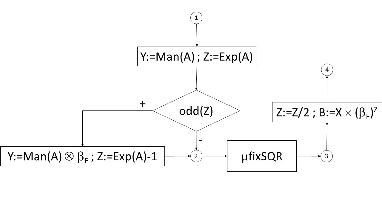
Figure 7: A flowchart of the square root algorithm $fltSQR$ for floating-point arithmetic

The algorithm $fltSQR$ to compute floating-point approximations of the square root function for floating-point argument is presented in Fig. 7. In this algorithm

• $mixSQR$ is the algorithm from Fig. 6,

• an “input” variable $A$ and the “output” variable $B$ are of the floating-point type $F$,

• another “input” variable $Eps$ has the fix-point type $T$,

• a variable $Z$ is of the fix-point type $T$ (but range within integers $Int_{T}$),

• a machine operation $\otimes$ is the fix-point multiplication (specified in the subsection 5.1),

• and, finally, a constant $\beta_{F}$ is the exponent base (i.e. a fixed integer of type $T$).

Recall that the algorithm $mixSQR$ uses (within its scope) its own “local” variables and a constant:

• the “output” and “input” variables $X$ and $Y$ are of the fix-point type $T$,

• the variables $K$ and $N$ are also of the fix-point type $T$ (but range within integers $Int_{T}$),

• the variable $Stp$ of the fix-point type $T$ is the step of indexes of the look-up table $root$;

• the look-up table $root$ is an array of the fix-point type $T$ contains pre-computed upper approximations for square root for indexes;

• and a constant $\delta_{T}$ is the step of the fix-point type $T$ (i.e. a fixed real value of type $T$ that is the minimal positive value of this type).

Specification of the algorithm $fltSQR$ follows below:

$$\begin{array}[]{c}[A\in Val_{F}\ \&\ Y>0\ \&\ Eps\in Val_{T}\ \&\ Eps>0\ \&\\ \hskip 8.61108pt\&\ EPS\geq 2\delta_{T}(2+\log_{2}\frac{Stp}{Eps})\ \&\\ \&\ \mathbf{STEP}\ \&\ \mathbf{ROOT}\ \&\ \mathbf{ROUND}]\\ fltSQR\ [|B-\sqrt{A}|<\big{(}Eps+\frac{\delta_{T}}{2\sqrt{\beta_{F}}}\big{)}\times\beta^{\lfloor\frac{Exp(A)}{2}\rfloor}],\end{array}$$ (16)

where $\lfloor\dots\rfloor$ is integer round-down function.

The assertion is easy to verify since the algorithm $mixSQR$ is verified already and the algorithm $fltSQR$ has loop-free flowchart (since the only loop is hidden inside $mixSQR$ in this chart). The only thing we need are annotations for control points on the chart:

1. the precondition from (16);

2. the precondition from (15) extended by the following two conjuncts:

   1. $Y=\ if\ odd(Exp(A))\ then\ Man(A)\otimes\beta_{F}\ else\ Man(A)$;

   2. $Z=\ if\ odd(Exp(A))\ then\ (Exp(A)-1)\ else\ Exp(A)$;

3. the postcondition from (15) extended by the same two conjuncts 2a and 2b;

4. the postcondition from (16).

Proof of the paths (1+2) and (1–2) are straightforward.

Let us proof the path (2..3). For it let us assume that the condition assigned to the control point 2 is true. It implies that before exercise of $mixSQR$ the precondition in (15) is true; due to the correctness of the assertion (15), the algorithm $mixSQR$ terminates and upon its termination the postcondition in (15) is true also. Remark also that conjuncts 2a and 2b remains true since $mixSQR$ doesn’t change neither $Y$ nor $A$. Hence the condition assigned to the control point 3 is true. It finishes the proof of the path (2..3).

For proving the last path (3..4) firstly let us prove that the condition in the control point (3) implies the next two properties:

$$\frac{Z}{2}=\lfloor\frac{Exp(A)}{2}\rfloor,$$ (17)

$$\begin{array}[]{c}|X-\sqrt{if\ odd(Exp(A))\ then\ Man(A)\times\beta_{F}\ else\ Man(A)}|\ <\\ \hskip 227.62204pt<\ \big{(}Eps+\frac{\delta_{T}}{2\sqrt{\beta_{F}}}\big{)}.\end{array}$$ (18)

The first property (17) directly follows from the condition (2b). The prove of the second one follows below:

$Exp(a)$ is even:

The radicand and the variable $Y$ (in algorithm $mixSQR$) both equal $Man(A)$; hence

$|X-\sqrt{if\ odd(Exp(A))\ then\ Man(A)\otimes\beta_{F}\ else\ Man(A)}|\ =$

$=\ |X-\sqrt{Y}|\ <$ (because assertion (15) is correct)$<$

$<\ Eps\ <\ \big{(}Eps+\frac{\delta_{T}}{2\sqrt{\beta_{F}}}\big{)}$.

$Exp(a)$ is odd:

The radicand equals $Man(A)\times\beta_{F}$ and the variable $Y$ equals $Man(A)\otimes\beta_{F}$; hence

$|X-\sqrt{if\ odd(Exp(A))\ then\ Man(A)\times\beta_{F}\ else\ Man(A)}|\ =$

$=\ |X-\sqrt{Man(A)\times\beta_{F}}|\ <$

$<\ |X-\sqrt{Man(A)\otimes\beta_{F}}|\ +\ |\sqrt{Man(A)\otimes\beta_{F}}-\sqrt{Man(A)\times\beta_{F}}|\ <$

(due to correctness of the assertion (15))

$<\ Eps\ +|\sqrt{Man(A)\otimes\beta_{F}}-\sqrt{Man(A)\times\beta_{F}}|<$

(because of properties of the fix-point arithmetic, where $|\Delta|<\frac{\delta_{T}}{2}$)

$<\ Eps\ +|\sqrt{Man(A)\times\beta_{F}+\Delta}-\sqrt{Man(A)\times\beta_{F}}|<$

(because of Taylor expansion of $\sqrt{t+\Delta}$ as a series $\sqrt{t}+\frac{\Delta}{\sqrt{t}}+\dots$) $<\ Eps\ +|\sqrt{Man(A)\times\beta_{F}}+\frac{\Delta}{\sqrt{Man(A)\times\beta_{F}}}+...-\sqrt{Man(A)\times\beta_{F}}|<$

$<\ Eps\ +|\frac{\Delta}{\sqrt{Man(A)\times\beta_{F}}}+...|<$

(because the Taylor expansion of $\sqrt{t+\Delta}$ is an alternating series)

$<\ Eps\ +|\frac{\delta_{T}}{2\sqrt{Man(A)\times\beta_{F}}}|<$

$<$(because $1<Man(A)$)$<\ Eps\ +\frac{\delta_{T}}{2\sqrt{\beta_{F}}}$.

As soon as it is proved that the properties (17) and (18) are valid in the control point (3), the proof of the path (3..4) become trivial.

It finishes pen-and-paper verification of specified algorithm computing approximations for the square root with floating-point arithmetic.

8 Conclusion

Let us summarise the content of the paper.

Firstly we take a very standard Newton method to compute square root, present is as an iterative algorithm $SQR$, specify it by Hoare total correctness assertion, and prove its validity in the case when input argument is greater than 1, accuracy is positive, and “computer” is precise (i.e. all computations are done in mathematical real numbers); the upper bound of loop iterations of the algorithm $SQR$ is logarithmic.

Next we improve the algorithm $SQR$ by using an auxiliary function to compute better initial approximations for square roots (it results in the algorithm $ISQR$) and then suggest a for-loop-based algorithm $FSQR$ that uses the same auxiliary function, computes a lower bound for the number of iterations that is sufficient to achieve the specified accuracy; both algorithms $ISQR$ and $FSQR$ work with precise arithmetic, but we prove that $FSQR$ achieves better accuracy than $ISQR$, and can achieves better accuracy if to increase the number of the loop iterations.

Then we convert for-loop-based algorithm with precise arithmetic $FSQR$ into algorithm $fixSQR$ with fix-point arithmetic, specify it by total correctness assertion and prove its validity by adjustment of its runs with runs of $FSQR$ with the same input data. Another specifics of the algorithm $fixSQR$ is use a look-up table (arrange as an array) for upper approximations of square roots and rounding-up function.

Use of a machine fix-point arithmetic instead of the precise arithmetic results in situation that more iterations of the loop doesn’t always improve accuracy in contrast to $FSQR$. Due to this reason we suggest an other algorithm $mixSQR$ that is a specialised version of the algorithm $fixSQR$.

Finally we use the algorithm $mixSQR$ as a subroutine in algorithm $fltSQR$ that computes approximations of the square root function in floating-point arithmetic. For this we assume that each floating-point number is represented as its mantissa and exponent, and both — the mantissa and exponent — are fix-point numbers. We specify the algorithm by a total correctness assertion and prove its correctness (basing on the correctness of the algorithm $mixSQR$).

All proofs in this paper are human-driven and oriented pen-and-paper proofs. So the next topic of our project is to validate all these proofs with aid of some automated proof-assistant. We are going to use ACL2 due to industrial strength of this proof-assistant [13] for platform-specific verification of the standard mathematical functions (but don’t rule out alternatives to this assistant).

Nevertheless remark that we attempt and present in this paper an approach that we call platform-independent. Also remark that we don’t attempt to build an axiomatization of an “abstract” machine (fix-point or floating-point) arithmetics. Instead we just make several explicit assumptions about machine arithmetic (and how it relates to the precise arithmetic) that are sufficient to validate specifications and algorithms with machine arithmetic by using its relations with specifications and algorithms with precise arithmetics. We believe that our assumptions about machine arithmetic are valid for many platforms and they are easy to check. Remark that if a platform’s machine arithmetic meets these assumptions then properties of the algorithms $mixSQR$ and $fltSQR$ exercised on this platform are specified by total correctness assertions (15) and (16) respectively.

Let us group together and list in one place our assumptions about fix-point and floating-point machine arithmetic that we introduce in the subsection 5.1 and the section 7) and use in this paper:

Fix-point arithmetic:

We understand fix-point numeric data type $T$ as follows:

• the set of values $Val_{T}$ is a finite subset of mathematical reals $\mathbb{R}$ such that

  • it comprises all reals in some finite range $[-\inf_{T},\sup_{T}]$, where $\inf_{T}>2$, $\sup_{T}>2$, with some fixed step $\frac{1}{2}>\delta_{T}>0$,

  • and includes all integer numbers $Int_{T}$ in this range $[-\inf_{T},\sup_{T}]$;

• legal binary arithmetic operations are

  • addition and subtraction; if not the range overflow exception then these operations are precise: they equal to the standard mathematical operations assuming their mathematical results fall in the range $[-\inf_{T},\sup_{T}]$ (and due to this reason are denoted as $+$ and $-$);

  • multiplication $\otimes$ and division $\oslash$; these operations are approximate but correctly rounded in the following sense: for all $x,y\in Val_{T}$

    • if $x\times y\in Val_{T}$ then $x\otimes y=x\times y$;

    • if $x/y\in Val_{T}$ then $x\oslash y=x/y$;

    • if $x\times y\in[-\inf_{T},\sup_{T}]$ then $|x\otimes y-x\times y|<\delta_{T}/2$;

    • if $x/y\in[-\inf_{T},\sup_{T}]$ then $|x\oslash y-x/y|<\delta_{T}/2$.

• legal binary relations are equality and all standard inequalities; these relations are precise, i.e. they equal to the standard mathematical relations (and due to this reason are denoted as $=$, $\neq$, $\leq$, $\geq$, $<$, $>$).

Floating-point arithmetic

We understand floating-point numeric data type $F$ as follows:

• the set of values $Val_{F}$ is a finite subset of mathematical reals $\mathbb{R}$ that comprises some reals in some finite range $[-\inf_{F},\sup_{F}]$, where $\inf_{F},\sup_{F}>2$ and $\{0,\inf_{F},\sup_{F}\}\subseteq Val_{F}$;

• there are two unary operations $Man:Val_{F}\rightarrow Val_{T}$ (called mantissa), $Exp:Val_{F}\rightarrow Int_{T}$ (called exponent), and an integer constant $\beta_{T}\in Int_{F}$ (called exponent base or just base) such that for all positive $x\in Val_{F}$

  • $1<Man(x)<\frac{sup_{T}}{\beta_{F}}$;

  • if $inf_{T}$ is odd then $-inf_{T}<Exp(x)$ else $-inf_{T}\leq Exp(x)$;

  • $x=Man(x)\times\beta_{F}^{Exp(x)}$.

Let us remark that our fix-point and floating-point numeric types are internal or instant types in the following sense:

• a program language provides numeric user-types integer, real, etc. (they may be int and/or long int, float and/or double in C, or integer and real in Pascal, etc.) with type-, implementation-, and platform-dependent the unit of least precision (or unit in the last place) $ulp_{\tau}\in\mathbb{R}$, where $\tau$ is a “complex parameter” (type, implementation, platform);

• our fix-point type $T$ and floating-point type $F$ are types for microprograms to implement algorithms $mixSQR$ and $fltSQR$ in such a way that there exist values $\varepsilon>0$ and $s>0$ for variables $Eps$ and $Stp$ that guaranty exact accuracy of the implemented $mixSQR$ and $fltSQR$, (i.e. $\frac{ulp_{\tau}}{2}>\varepsilon$ in the case of integer and algorithm $mixSQR$, and $\frac{ulp_{\tau}}{2}>\varepsilon+\frac{\delta_{T}}{2\sqrt{\beta_{F}}}$ in the case of real and algorithm $fltSQR$).

Finally let us mention one more research topic — to find an “optimal balance” between size of the array $root$ with initial upper approximations for square roots for selected arguments, number of iterations of the loop in the algorithm $finSQR$, and accuracy of the square root approximation: if $\varepsilon$ and $s$ are values of the variables $Eps$ and $Stp$ then the array size is $\frac{\sup_{T}}{s}$, number of iterations may be any $n\geq\big{(}1+\lceil\log_{2}\frac{s}{\varepsilon}\rceil\big{)}$, and accuracy $|X-\sqrt{Y}|$ is less than $\big{(}\frac{s}{2^{n}}\ +\ n\times\delta_{T}\big{)}$.

Appendix 0.A Specification of the sqrt function

The C reference portal at en.cppreference.com/w/c specifics the the square root function sqrt [25] as it represented below.

C Numerics Common mathematical functions

sqrt, sqrtf, sqrtl

Defined in header $<$math.h$>$

float sqrtf( float arg ); (1) (since C99)

double sqrt( double arg ); (2)

long double sqrtl( long double arg ); (3) (since C99)

Defined in header $<$tgmath.h$>$

$\sharp$define sqrt( arg ) (4) (since C99)

1-3) Computes square root of arg.

4) Type-generic macro: If arg has type long double, sqrtl is called.

Otherwise, if arg has integer type or the type double, sqrt is called.

Otherwise, sqrtf is called. If arg is complex or imaginary,

then the macro invokes the corresponding complex function

(csqrtf, csqrt, csqrtl).

Parameters

arg - floating point value

Return value

If no errors occur, square root of arg ($\sqrt{arg}$), is returned.

If a domain error occurs, an implementation-defined value is returned

(NaN where supported).

If a range error occurs due to underflow, the correct result (after rounding)

is returned.

Error handling

Errors are reported as specified in math_errhandling.

Domain error occurs if arg is less than zero.

If the implementation supports IEEE floating-point arithmetic (IEC 60559),

$\bullet$ If the argument is less than $-0$, FE_INVALID is raised and NaN is returned.

$\bullet$ If the argument is $+\infty$ or $\pm$0, it is returned, unmodified.

$\bullet$ If the argument is NaN, NaN is returned

Notes

sqrt is required by the IEEE standard be exact.

The only other operations required to be exact are the arithmetic operators

and the function fma. After rounding to the return type

(using default rounding mode),

the result of sqrt is indistinguishable from the infinitely precise result.

In other words, the error is less than $0.5$ ulp.

Other functions, including pow, are not so constrained.

References

- [1] Ayad A., Marché C. Multi-prover verification of floating-point programs // Lecture Notes in Artificial Intelligence. 2010. Vol. 6173. P.127–141.
- [2] Barret G. 1989. Formal Methods Applied to a Floating-Point Number System // IEEE Trans. Softw. Eng. 1989. Vol. 15(5). P.611–621.
- [3] Brain M., Tinelli C., Ruemmer Ph., and Wahl T. An Automatable Formal Semantics for IEEE-754 Floating-Point Arithmetic // Proceedings of the 2015 IEEE 22nd Symposium on Computer Arithmetic (ARITH ’15). IEEE Computer Society. 2015. P160–167.
- [4] Ferguson W.E. (Jr), Bingham J., Erkok L., Harrison J.R., Leslie-Hurd J. Digit serial methods with applications to division and square root (with mechanically checked correctness proofs) // 2017. Eprint arXiv:1708.00140. https://arxiv.org/abs/1708.00140. (Visited December 19, 2017.)
- [5] Gamboa R.A. Square Roots in Acl2: a Study in Sonata Form // Technical Report. University of Texas at Austin, USA. 1997.
- [6] Gries D. The Science of Programming. Springer-Verlag, 1981.
- [7] Harrison J. A Machine-Checked Theory of Floating Point Arithmetic // Lecture Notes in Computer Science. 1999. Vol. 1690. P. 113–130.
- [8] Harrison J. Formal Verification of Floating Point Trigonometric Functions // Lecture Notes in Computer Science. 2000. Vol. 1954. P.217-233.
- [9] Harrison J. Formal Verification of IA-64 Division Algorithms // Lecture Notes in Computer Science. 2000. Vol. 1869. P. 233–251.
- [10] Harrison J. Floating Point Verification in HOL Light: The Exponential Function // Formal Methods System Design. 2000. Vol. 16(3). P. 271–305.
- [11] Harrison J. Formal Verification of Square Root Algorithms // Formal Methods in System Design. 2003. Vol. 22(2). P.143–153.
- [12] Hoare C.A.R. The Verifying Compiler: A Grand Challenge for Computing Research // Lecture Notes in Computer Science. 2003. Vol. 2890. P. 1–12.
- [13] Grohoski G. Verifying Oracle’s SPARC Processors with ACL2. Slides of the Invited talk for 14th International Workshop on the ACL2 Theorem Prover and Its Applications. http://www.cs.utexas.edu/users/moore/acl2/workshop-2017/slides-accepted/grohoski-ACL2_talk.pdf. (Visited December 19, 2017.)
- [14] Gutowski M.W. Power and beauty of interval methods. arXiv:physics/0302034 [physics.data-an]. http://arxiv.org/pdf/physics/0302034.pdf. (Visited December 19, 2017.)
- [15] Kochan S.G. Programming in C: A Complete Introduction to the C Programming Language. Functions Calling Functions at p.131. Sam’s Publishing, 2005 (3rd Edition).
- [16] Kuliamin V. Standardization and Testing of Mathematical Functions // Programming and Computer Software. 2007. Vol. 33, n. 3. P. 154–173.
- [17] Kuliamin V.V. Standardization and Testing of Mathematical Functions in floating point numbers // Lecture Notes in Computer Science. 2010. Vol. 5947. P. 257–268.
- [18] Monniaux D. The pitfalls of verifying floating-point computations // ACM Transactions on Programming Languages and Systems. 2008. Vol. 30, n. 3. P.1–41.
- [19] Muller J.-M. Elementary Functions: Algorithms and Implementation. Birkhauser, 2005.
- [20] Sawada J., Gamboa R. Mechanical Verification of a Square Root Algorithm Using Taylor’s Theorem // Lecture Notes in Computer Science. 2002. Vol. 2517. P. 274–291.
- [21] Shelihov V.I. Verification and synthesis of efficient programs for standard functions flor, isqrt and ilog2 using predicate programming technology // Proceedings of 12 Int. Conf. on Control and modelling of complex systems. Samara: Samara Science Center of Russian Academy of Science. 2010. P.622-630. (In Russian.)
- [22] Shilov N.V. On the need to specify and verify standard functions // The Bulletin of the Novosibirsk Computing Center (Series: Computer Science). 2015. n.38, p.105–119.
- [23] Shilov N.V., Promsky A.V. On specification andd verification of standard mathematical functions // Humanities and Science University Journal. 2016. n.19, p.57–68.
- [24] Siddique U., Hasan O. On the Formalization of Gamma Function in HOL // 2014. J. Autom. Reason. Vol. 53(4). P. 407–429.
- [25] C refernce. Sqrt, sqrtf, sqrtl. http://en.cppreference.com/w/c/numeric/math/sqrt. (Visited December 19, 2017.)
- [26] IEEE 754-2008. http://ieeexplore.ieee.org/document/4610935. (Visited December 19, 2017.)
- [27] ISO/IEC/IEEE 60559:2011. Information technology -- Microprocessor Systems -- Floating-Point arithmetic http://www.iso.org/iso/iso_catalogue/catalogue_tc/catalogue_detail.htm?csnumber=57469. (Visited December 19, 2017. In Russian.)
- [28] Roskosmos called the reason of unsuccessful start from the East spaceport https://news.mail.ru/politics/31931345/. (Visited December 19, 2017.)