Phase Transition of Convex Programs for Linear Inverse Problems with Multiple Prior Constraints

Abstract

A sharp phase transition emerges in convex programs when solving the linear inverse problem, which aims to recover a structured signal from its linear measurements. This paper studies this phenomenon in theory under Gaussian random measurements. Different from previous studies, in this paper, we consider convex programs with multiple prior constraints. These programs are encountered in many cases, for example, when the signal is sparse and its $\ell_{2}$ norm is known beforehand, or when the signal is sparse and non-negative simultaneously. Given such a convex program, to analyze its phase transition, we introduce a new set and a new cone, called the prior restricted set and prior restricted cone, respectively. Our results reveal that the phase transition of a convex problem occurs at the statistical dimension of its prior restricted cone. Moreover, to apply our theoretical results in practice, we present two recipes to accurately estimate the statistical dimension of the prior restricted cone. These two recipes work under different conditions, and we give a detailed analysis for them. To further illustrate our results, we apply our theoretical results and the estimation recipes to study the phase transition of two specific problems, and obtain computable formulas for the statistical dimension and related error bounds. Simulations are provided to demonstrate our results.

I Introduction

The linear inverse problem refers to the problem of recovering an unknown signal from its linear measurements. It is frequently encountered in many applications, such as image processing [1], network data analysis [2] and so on. In practice, we often have less measurements than the dimension of the true signal. As a result, the problem is generally ill-posed. Therefore, to make recovery possible, we may assume that the true signal has low complexity under some structures. Commonly considered structures include sparsity and low rank, and the corresponding recovery problems are known as compressed sensing and matrix completion.

Given the structures of the signal, a popular approach for recovery is to solve a convex program that enforces the known prior information about the structures. For example, we pursue a sparse recovery through $\ell_{1}$ norm minimization in the compressed sensing problem, and a low-rank recovery through nuclear norm minimization in the matrix completion problem. This approach is shown to be simple and efficient in many practical applications.

Meanwhile, a sharp phase transition is numerically observed, when we use convex programs to recover structured signals. The phase transition refers to the phenomenon that for a certain convex program, when the measurement number is greater than some threshold, it succeeds with high probability; while when the measurement number is smaller than another threshold, it fails with high probability. When we say a sharp phase transition, we mean that the transition region is very narrow. This phenomenon has attracted many researchers, and much work has been done to explain it in theory in the past several years. Some exciting results have been obtained since then.

In [3, 4, 5, 6], Donoho and Tanner analyzed the phase transition of the compressed sensing problem in the asymptotic regime. They first demonstrated that the $\ell_{1}$ minimization approach succeeds if and only if the random projection preserves the structure of faces of cross-polytope, and then used the theory of polytope angles to deal with this problem. In [7, 8, 9], the authors established a connection between the phase transition and the statistical decision theory, and revealed that the phase transition curve coincides with the minimax risk curve of denoising in many linear inverse problems. In [10], Amelunxen et al. presented a comprehensive analysis of the phase transition of convex programs in the linear inverse problem. They first formulated the phase transition problem to a geometry problem, then used tools from the theory of conic integral geometry to study this geometry problem. The results show that the phase transition of convex programs occurs at the statistical dimension of the descent cone of the structure inducing function at the true signal. In [11], Rudelson and Vershynin studied the performance of the $\ell_{1}$ minimization approach using the “escape from the mesh” theorem [12] in Gaussian process theory. Later, their ideas were extended in the papers [13, 14, 10], and the phase transition were identified by incorporating the arguments of Rudelson and Vershynin with a polarity argument. The obtained results are stated in terms of Gaussian width, and consistent with the results in [10]. In [15], Bayati et al. made use of a state evolution framework, inspired by ideas from statistical physics, and demonstrated that the phase transition of $\ell_{1}$ minimization is universal over a class of sensing matrices. Recently, in [16], Oymak and Tropp demonstrated the universality laws for the phase transition of convex programs for linear inverse problems, over a class of sensing matrices.

However, most of the above work focuses on the case when we have no additional prior constraints. But in many practical problems, we do have some additional prior information. For example, in image processing problems, in addition to the structures about texture etc, the fact that the pixel values are non-negative may help to recover the true image. In these cases, we would solve convex problems with (multiple) prior constraints to recover the true signal. While these problems exhibit a sharp phase transition as well, theoretical understanding of the phase transition is far from satisfactory. We mention that in [3, 4], Donoho and Tanner studied the $\ell_{1}$ minimization problem with an additional non-negativity constraint, and “weak threshold” and “strong threshold” were obtained in the asymptotic regime, which marks the phase transition. Nevertheless, a comprehensive analysis about the phase transition of this problem does not exist. Furthermore, when the signal has structures other than sparsity, or when we have prior constraints other than non-negativity, it remains an open problem to prove the existence and identify the location of the phase transition.

In this paper, we study the phase transition of convex programs with multiple prior constraints under Gaussian random measurements. In our analysis, we first introduce a new set and a new cone, called the prior restricted set and prior restricted cone, respectively. Next, we give a sufficient and necessary condition for the success of convex programs, which involves the prior restricted cone. It states that convex programs succeed if and only if the intersection of the null space of the sensing matrix and the prior restricted cone contains only the origin. This condition has been well studied by Amelunxen et al. in [10] using the theory of conic integral geometry. Utilizing their results, we obtain that the phase transition of convex programs with multiple prior constraints occurs at the statistical dimension of the prior restricted cone. Thus, intuitively, the “dimension” of the prior restricted cone (i.e., the statistical dimension of this cone) can be seen as a measure of how much we know about the true signal from the prior information, if convex programs are used to recover signals. Moreover, to apply our theoretical results in practice, we present two recipes to accurately estimate the statistical dimension of the prior restricted cone. The two recipes work under different conditions, and we give a detailed analysis for them. To further illustrate our results, we apply our theoretical results and the estimation recipes to study the phase transition of two specific problems: One is the linear inverse problem with $\ell_{2}$ norm constraints, and the other is the linear inverse problem with non-negativity constraints. We obtain computable formulas for the statistical dimension and related error bounds in either problem. The following simulations demonstrate that our results match the empirical successful probability perfectly.

The rest of the paper is organized as follows: In section II, we give a precise statement of the problems studied in this paper. In section III, some preliminaries and notations are introduced. In section IV, we state our main results. In section V, we apply our main results to study the phase transition of two specific problems. In section VI, simulations are provided to demonstrate our theoretical results. In section VII, we conclude the paper.

II Problem Formulation

In this section, we provide a precise statement of the problems studied in this paper. In section II-A, we introduce the linear inverse problem. In section II-B, we introduce the convex optimization procedure to recover signals from compressed, linear measurements.

II-A Linear Inverse Problem

In the linear inverse problem, we observe a signal via its linear measurements:

$$\bm{y}=\bm{A}\bm{x}^{\star},$$ (1)

where $\bm{y}\in\mathbb{R}^{m}$ is the measurement vector, $\bm{A}\in\mathbb{R}^{m\times n}$ is the sensing matrix, and $\bm{x}^{\star}\in\mathbb{R}^{n}$ is the unknown signal. Our goal is to recover $\bm{x}^{\star}$ given the knowledge of $\bm{y}$ and $\bm{A}$.

II-B Convex Optimization Procedure

In many applications, we often have compressed measurements, i.e., $m<n$. As a result, to recovery $\bm{x}^{\star}$ from $\bm{y}$ and $\bm{A}$ is an ill-posed problem. Hence, to make recovery possible, it is commonly assumed that the signal $\bm{x}^{\star}$ is well structured. In this case, a simple yet efficient approach for recovery is to solve a convex program, which forces the solution to have the corresponding structures. Moreover, apart from the assumed structures, we may have some additional prior information about $\bm{x}^{\star}$. For example, we may know the $\ell_{2}$ norm of $\bm{x}^{\star}$ beforehand, or the signal $\bm{x}^{\star}$ is non-negative. The additional prior information often acts as constraints.

Suppose that $f_{0}:\mathbb{R}^{n}\rightarrow\overline{\mathbb{R}}$ is a proper convex function and promotes the structures of $\bm{x}^{\star}$, and $f_{i}:\mathbb{R}^{n}\rightarrow\overline{\mathbb{R}},1\leq i\leq k,$ are some proper convex functions and promote the additional prior information of $\bm{x}^{\star}$. Then in practice the following convex program is often used to recover the true signal $\bm{x}^{\star}$:

$$\min f_{0}(\bm{x}),\quad\operatorname*{s.t.}\ \bm{y}=\bm{A}\bm{x},\ f_{i}(\bm{x})\leq f_{i}(\bm{x}^{\star}),\ i=1,\dots,k.$$ (2)

We say that the convex problem (2) succeeds if the unique solution $\hat{\bm{x}}$ satisfies $\hat{\bm{x}}=\bm{x}^{\star}$; otherwise, we say it fails.

In this paper, we study the phase transition of problem (2). The analysis relies on some knowledge from convex analysis and convex geometry. Hence, in the next section, we give a brief introduction about the needed knowledge.

III Preliminaries

In this section, we present some preliminaries that will be used in our analysis.

III-A Subgradient

Suppose $h:\mathbb{R}^{n}\rightarrow\overline{\mathbb{R}}$ is a proper convex function. Then the subdifferential of $h$ at $\bm{z}\in\mathbb{R}^{n}$ is the set

$$\partial h(\bm{z})=\big{\{}\bm{u}\in\mathbb{R}^{n}:h(\bm{z}+\bm{t})\geq h(\bm{z})+\left<\bm{u},\bm{t}\right>\ \textnormal{for all}\ \bm{t}\in\mathbb{R}^{n}\big{\}}.$$

III-B Descent Cones and Normal Cones of Convex Functions

The descent cone of a proper convex function $h:\mathbb{R}^{n}\rightarrow\overline{\mathbb{R}}$ at $\bm{z}\in\mathbb{R}^{n}$ is the set of all non-ascent directions of $h$ at $\bm{z}$:

$$D(h,\bm{z})=\big{\{}\bm{d}\in\mathbb{R}^{n}:\exists\,a>0,h(\bm{z}+a\cdot\bm{d})\leq h(\bm{z})\big{\}}.$$

The normal cone of a proper convex function $h:\mathbb{R}^{n}\rightarrow\overline{\mathbb{R}}$ at $\bm{z}\in\mathbb{R}^{n}$ is the polar of the descent cone of $h$ at $\bm{z}$:

$$N(h,\bm{z})=D(h,\bm{z})^{\circ}=\big{\{}\bm{u}\in\mathbb{R}^{n}:\left<\bm{u},\bm{d}\right>\leq 0\ \textnormal{for all}\ \bm{d}\in D(h,\bm{z})\big{\}}.$$

Suppose $\partial h(\bm{z})$ is non-empty, compact, and does not contain the origin, then the normal cone is the cone generated by the subdifferential [17, Corollary 23.7.1]:

$$N(h,\bm{z})=\operatorname{cone}\big{(}\partial h(\bm{z})\big{)}=\big{\{}\bm{u}\in\mathbb{R}^{n}:\exists\,\tau\geq 0,\bm{u}\in\tau\cdot\partial h(\bm{z})\big{\}}.$$

III-C Normal Cone to Convex Sets

Let $C\subseteq\mathbb{R}^{n}$ be a convex set with $\bar{\bm{x}}\in C$. The normal cone to $C$ at $\bar{\bm{x}}$ is

$$N(\bar{\bm{x}};C)\coloneqq\{\bm{v}\in\mathbb{R}^{n}:\ \left<\bm{v},\bm{x}-\bar{\bm{x}}\right>\leq 0,\ \forall\,\bm{x}\in C\}.$$

III-D Statistical Dimension of Convex Cones

For a convex cone $K$, the statistical dimension of $K$ is defined as:

$$\delta(K)=\mathbb{E}\Big{(}\sup_{\bm{t}\in K\cap\mathbb{B}^{n}}\left<\bm{g},\bm{t}\right>\Big{)}^{2},\text{ where }\bm{g}\sim N(\bm{0},\bm{I}_{n}).$$

The statistical dimension of a convex cone has a number of important properties, see [10, Proposition 3.1]. Moreover, the statistical dimension satisfies the following additivity property:

Fact 1 (Additivity of statistical dimension).

Let $K_{1}$ and $K_{2}$ be two convex cones in $\mathbb{R}^{n}$. The following holds:

1. If for any $\bm{a}\in K_{1}$ and $\bm{b}\in K_{2}$, we have $\left<\bm{a},\bm{b}\right>=0$. Then

   $$\delta(K_{1}+K_{2})=\delta(K_{1})+\delta(K_{2}).$$

2. If for any $\bm{a}\in K_{1}$ and $\bm{b}\in K_{2}$, we have $\left<\bm{a},\bm{b}\right>\leq 0$. Then

   $$\delta(K_{1}+K_{2})\geq\delta(K_{1})+\delta(K_{2}).$$

3. If for any $\bm{a}\in K_{1}$ and $\bm{b}\in K_{2}$, we have $\left<\bm{a},\bm{b}\right>\geq 0$. Then

   $$\delta(K_{1}+K_{2})\leq\delta(K_{1})+\delta(K_{2}).$$

Proof.

See Appendix F. ∎

Fact 1 generalizes the fact that for two linear subspaces $L_{1}$ and $L_{2}$, suppose $L_{1}\perp L_{2}$, then $\dim(L_{1}+L_{2})=\dim(L_{1})+\dim(L_{2})$, since the statistical dimension extends the dimension of a linear subspace to the class of convex cones [10].

III-E Indicator Function of a Convex Set

Let $C\subseteq\mathbb{R}^{n}$ be a convex set. Then the indicator function of the set $C$ is defined as

$$I_{C}(\bm{x})=\left\{\begin{array}[]{cl}0,&\textnormal{when}\ \bm{x}\in C,\\ \infty,&\textnormal{when}\ \bm{x}\notin C.\end{array}\ \right.$$

For any $\bar{\bm{x}}\in C$, the subdifferential of $I_{C}$ is [18, Example 2.32]:

$$\partial I_{C}(\bar{\bm{x}})=N(\bar{\bm{x}};C)=\{\bm{v}\in\mathbb{R}^{n}:\left<\bm{v},\bm{x}-\bar{\bm{x}}\right>\leq 0,\ \forall\,\bm{x}\in C\}.$$ (3)

III-F Prior Restricted Set and Prior Restricted Cone

We first define the prior restricted set of convex problem (2):

Definition 1 (Prior Restricted Set).

For the convex problem (2), suppose $\bm{x}^{\star}\in\mathbb{R}^{n}$ is the true signal, then we define its prior restricted set as the following set:

$$\mathcal{S}=\big{\{}\bm{d}\in\mathbb{R}^{n}:f_{i}(\bm{x}^{\star}+\bm{d})\leq f_{i}(\bm{x}^{\star}),\ i=0,1,\dots,k\big{\}}.$$

Using this set, we can define the prior restricted cone of problem (2):

Definition 2 (Prior Restricted Cone).

For the convex problem (2), suppose $\bm{x}^{\star}\in\mathbb{R}^{n}$ is the true signal, then we define its prior restricted cone as the following set:

$$\mathcal{C}=\operatorname{cone}(\mathcal{S})=\{\bm{u}\in\mathbb{R}^{n}:\exists\,t>0,f_{i}(\bm{x}^{\star}+t\cdot\bm{u})\leq f_{i}(\bm{x}^{\star}),\ i=0,1,\dots,k\}.$$

III-G Notations

Throughout, we denote $\mathbb{R}^{n}_{+}$ the non-negative orthant in $\mathbb{R}^{n}$: $\mathbb{R}^{n}_{+}\coloneqq\{\bm{x}\in\mathbb{R}^{n}:\bm{x}_{i}\geq 0\ \textnormal{for}\ 1\leq i\leq n\}$, and $\mathbb{R}^{n}_{++}$ the positive part: $\mathbb{R}^{n}_{++}\coloneqq\{\bm{x}\in\mathbb{R}^{n}:\bm{x}_{i}>0\ \textnormal{for}\ 1\leq i\leq n\}$.

For a set $C\in\mathbb{R}^{n}$, we use $\operatorname{int}(C)$ to denote its interior:

$$\operatorname{int}(C)\coloneqq\{\bm{x}\in C:\mathbb{B}(\bm{x},r)\subseteq C\ \textnormal{for some}\ r>0\}.$$

Denote $\operatorname{aff}(C)$ the affine hull of $C$:

$$\operatorname{aff}(C)=\{\theta_{1}\bm{x}_{1}+\dots+\theta_{k}\bm{x}_{k}:\,\bm{x}_{1},\dots,\bm{x}_{k}\in C,\ \theta_{1}+\dots+\theta_{k}=1\},$$

and $\operatorname{ri}(C)$ the relative interior of the set $C$:

$$\operatorname{ri}(C)=\{\bm{x}\in C:\,\mathbb{B}(\bm{x},r)\cap\operatorname{aff}(C)\subseteq C\ \textnormal{for some}\ r>0\}.$$

The closure of $C$ is denoted by either $\overline{C}$ or $\operatorname{cl}(C)$.

Given a point $\bm{u}\in\mathbb{R}^{n}$ and a subset $C\subseteq\mathbb{R}^{n}$, the distance of $\bm{u}$ to the set $C$ is denoted by $\operatorname{dist}(\bm{u},C)$:

$$\operatorname{dist}(\bm{u},C)\coloneqq\inf_{\bm{x}\in C}\|\bm{u}-\bm{x}\|_{2}.$$

We denote $\Pi_{C}(\bm{u})$ the projection of $\bm{u}$ onto the set $C$:

$$\Pi_{C}(\bm{u}):=\{\bm{x}\in C:\|\bm{u}-\bm{x}\|_{2}=\operatorname{dist}(\bm{u},C)\}.$$

If $C$ is non-empty, convex, and closed, the projection $\Pi_{C}(\bm{u})$ is a singleton. In this case, $\Pi_{C}(\bm{u})$ may denote the unique point in it, depending on the context.

IV Main Results

In this section, we state our main results in this paper. We first give results about the phase transition of problem (2) in subsection IV-A, and then present two recipes to estimate the statistical dimension of the prior restricted cone in subsections IV-B and IV-C.

IV-A Phase Transition of Convex Programs with Multiple Prior Constraints

In this subsection, we state our main results about the phase transition of problem (2). We begin by a geometry condition which determines the success of problem (2):

Lemma 1 (Optimality condition).

Consider problem (2) to recover the true signal $\bm{x}^{\star}$. If $f_{i}$ is a proper convex function for any $0\leq i\leq k$, problem (2) succeeds if and only if

$$\mathcal{C}\cap\operatorname{null}(\bm{A})=\{\bm{0}\},$$

where $\mathcal{C}$ denotes the prior restricted cone of problem (2).

Proof.

See Appendix A. ∎

Fig. 1 gives a geometric interpretation of Lemma 1. Note that when there is no additional prior constraint, i.e., when we consider problem

$$\min f_{0}(\bm{x}),\quad\operatorname*{s.t.}\ \bm{y}=\bm{A}\bm{x}$$ (4)

to recover $\bm{x}^{\star}$, the prior restricted cone is exactly $D(f_{0},\bm{x}^{\star})$, the descent cone of $f_{0}$ at $\bm{x}^{\star}$. In this case, our optimality condition, Lemma 1, will degenerate to the optimality condition given by Chandrasekaran et al. in [13, Fact 2.8].

\begin{overpic}[scale={0.49}]{success_noise_free.eps} \put(90.0,44.0){\color[rgb]{0.547,0.161,0.161}{$\operatorname{null}(\bm{A})$}} \put(28.0,25.0){\color[rgb]{0.298,0.709,0.862}{$\mathcal{C}$}} \put(41.0,39.0){\color[rgb]{0.075,0.333,0.435}{$\mathcal{S}$}} \end{overpic}

\begin{overpic}[scale={0.49}]{failure_noise_free.eps} \put(69.0,3.0){\color[rgb]{0.547,0.161,0.161}{$\operatorname{null}(\bm{A})$}} \put(28.0,25.0){\color[rgb]{0.298,0.709,0.862}{$\mathcal{C}$}} \put(41.0,39.0){\color[rgb]{0.075,0.333,0.435}{$\mathcal{S}$}} \end{overpic}

Figure 1: A geometric interpretation of the optimality condition for success of problem (2), i.e., Lemma 1. In both figures, the dark red line denotes the null space of $\bm{A}$, the light blue region denotes the prior restricted cone of problem (2) (i.e., $\mathcal{C}$), and the dark blue region denotes the prior restricted set of problem (2) (i.e., $\mathcal{S}$). In figure (a), the intersection of $\operatorname{null}(\bm{A})$ and $\mathcal{C}$ contains only the origin. In this case, problem (2) succeeds. In figure (b), the intersection of $\operatorname{null}(\bm{A})$ and $\mathcal{C}$ contains a ray. In this case, problem (2) fails.

Using Lemma 1, we can study the phase transition of problem (2). For this purpose, we assume that we have random sensing matrix. In particular, we assume that $\bm{A}$ is drawn at random from the standard normal distribution on $\mathbb{R}^{m\times n}$. According to Lemma 1, to study the phase transition of problem (2), it is sufficient to answer the following questions:

• Under what conditions the kernel of $\bm{A}$ intersects the cone $\mathcal{C}$ trivially with high probability?

• Under what conditions the kernel of $\bm{A}$ intersects the cone $\mathcal{C}$ nontrivially with high probability?

This questions have been well studied in recent years. We borrow the answer from [10]:

Proposition 1 ([10], Theorem I).

Fix a tolerance $\zeta$. Suppose the matrix $\bm{A}\in\mathbb{R}^{m\times n}$ has independent standard normal entries, and $K$ denotes a convex cone. Then when

$$m\leq\delta(K)-a_{\zeta}\sqrt{n},$$

we have $\operatorname{null}(\bm{A})\cap K=\{\bm{0}\}$ with probability less than $\zeta$. On the contrary, when

$$m\geq\delta(K)+a_{\zeta}\sqrt{n},$$

we have $\operatorname{null}(\bm{A})\cap K=\{\bm{0}\}$ with probability at least $1-\zeta$. The quantity $a_{\zeta}\coloneqq\sqrt{8\log(4/\zeta)}$.

Proposition 1 is a direct consequence of [10, Theorem I]. The proof involves the theory of conic integral geometry. See reference [10] for details. Now combining Lemma 1 and Proposition 1, we obtain our main results about the phase transition:

Theorem 1 (Phase transition of convex programs with multiple prior constraints).

Consider convex problem (2) to solve the linear inverse problem. If the sensing matrix $\bm{A}$ has independent standard normal entries, the phase transition of problem (2) occurs at the statistical dimension of its prior restricted cone. More precisely, for any $\zeta>0$, when the measurement number $m$ satisfies

$$m\leq\delta(\mathcal{C})-a_{\zeta}\sqrt{n},$$

problem (2) fails with probability at least $1-\zeta$. On the contrary, when

$$m\geq\delta(\mathcal{C})+a_{\zeta}\sqrt{n},$$

problem (2) succeeds with probability at least $1-\zeta$. The quantity $a_{\zeta}\coloneqq\sqrt{8\log(4/\zeta)}$.

Since the phase transition occurs at the statistical dimension of the prior restricted cone, intuitively, we can see it as a measure of how much we know about the true signal from the prior information.

Remark 1.

We can apply our Theorem 1 to analyze the phase transition of problem (4). The prior restricted cone of problem (4) is exactly $D(f_{0},\bm{x}^{\star})$, the descent cone of $f_{0}$ at $\bm{x}^{\star}$. Thus, in this case, our Theorem 1 can be read as: The phase transition of problem (4) occurs at the statistical dimension of $D(f_{0},\bm{x}^{\star})$. This coincides with the results in [10, Theorem II].

IV-B Statistical Dimension of Prior Restricted Cones: Part I

In theory, Theorem 1 have revealed that the phase transition of problem (2) occurs at the statistical dimension of its prior restricted cone. However, if we want to apply these results in practice, we must find ways to compute the statistical dimension efficiently. For this purpose, in this subsection, we present a recipe that provides a reliable estimate for the statistical dimension of the prior restricted cone, when all the subdifferentials are compact and do not contain the origin. The idea is inspired by the recipe proposed by Amelunxen et al. [10, pp. 244-248] for the computation of the statistical dimension of a descent cone.

The basic idea for the recipe is that the statistical dimension of the prior restricted cone can be expressed in terms of its polar, which has a close relation with the normal cones, and furthermore, the subdifferentials, of the functions $f_{i}$’s, $0\leq i\leq k$. Let us first express the statistical dimension in terms of normal cones.

Lemma 2.

Consider problem (2) to recover the true signal $\bm{x}^{\star}$. Let $D(f_{i},\bm{x}^{\star}),N(f_{i},\bm{x}^{\star})$ denote the descent cone and normal cone of $f_{i}$ at $\bm{x}^{\star}$ for $0\leq i\leq k$, respectively. Suppose that

$$\operatorname{ri}\big{(}D(f_{0},\bm{x}^{\star})\big{)}\cap\operatorname{ri}\big{(}D(f_{1},\bm{x}^{\star})\big{)}\cap\dots\cap\operatorname{ri}\big{(}D(f_{k},\bm{x}^{\star})\big{)}\neq\emptyset.$$

Then the polar of the prior restricted cone can be expressed as follows:

$$\mathcal{C}^{\circ}=\sum_{i=0}^{k}N(f_{i},\bm{x}^{\star}),$$

and the statistical dimension of the prior restricted cone can be expressed as follows:

$$\delta(\mathcal{C})=\mathbb{E}\operatorname{dist}^{2}\big{(}\bm{g},\sum_{i=0}^{k}N(f_{i},\bm{x}^{\star})\big{)}.$$

Proof.

See Appendix B-A. ∎

Lemma 2 establishes connections between the prior restricted cone and the individual normal cones, but it does not allow us to compute the statistical dimension of the prior restricted cone efficiently. This can be done by incorporating the subdifferential expression for normal cones.

Theorem 2 (The statistical dimension of the prior restricted cone).

Let $\mathcal{C}$ be the prior restricted cone of problem (2), and let $\bm{x}^{\star}\in\mathbb{R}^{n}$ be the true signal. Assume that for any $0\leq i\leq k$, the subdifferential $\partial f_{i}(\bm{x}^{\star})$ is non-empty, compact, and does not contain the origin. Assume that the descent cones satisfy

$$\operatorname{ri}\big{(}D(f_{0},\bm{x}^{\star})\big{)}\cap\operatorname{ri}\big{(}D(f_{1},\bm{x}^{\star})\big{)}\cap\dots\cap\operatorname{ri}\big{(}D(f_{k},\bm{x}^{\star})\big{)}\neq\emptyset.$$

Define the function $J:\mathbb{R}^{k+1}_{+}\rightarrow\mathbb{R}$ to be

$$J(\bm{\tau})\coloneqq\mathbb{E}\Big{[}\operatorname{dist}^{2}\Big{(}\bm{g},\sum_{i=0}^{k}\bm{\tau}_{i}\cdot\partial f_{i}(\bm{x}^{\star})\Big{)}\Big{]},$$

where $\bm{g}\sim N(\bm{0},\bm{I}_{n})$. Then the statistical dimension of the prior restricted cone has the following upper bound:

$$\delta\big{(}\mathcal{C}\big{)}\leq\inf_{\bm{\tau}\in\mathbb{R}^{k+1}_{+}}J(\bm{\tau}).$$

The function $J(\bm{\tau})$ is convex, continuous, and continuously differentiable in $\mathbb{R}^{k+1}_{+}$. It attains its minimum in a compact subset of $\mathbb{R}^{k+1}_{+}$. Moreover, suppose that

$$\textnormal{the two sets }\sum_{i=0}^{k}\bm{\tau}_{i}\cdot\partial f_{i}(\bm{x}^{\star})\textnormal{ and }\sum_{i=0}^{k}\tilde{\bm{\tau}}_{i}\cdot\partial f_{i}(\bm{x}^{\star})\textnormal{ are not identical, for any }\bm{\tau}\neq\tilde{\bm{\tau}}\in\mathbb{R}^{k+1}_{+}.$$

Then the function $J(\bm{\tau})$ is strictly convex, and attains its minimum at a unique point. For the differential of $J$ at the boundary of $\mathbb{R}^{k+1}_{+}$, we interpret the partial derivative $\frac{\partial J}{\partial\bm{\tau}_{i}}$ similarly as the right derivative, if $\bm{\tau}_{i}=0$.

Proof.

Since the subdifferential is non-empty, compact, and does not contain the origin, the normal cones is the cone generated by the subdifferential [17, Corollary 23.7.1]. Thus, by Lemma 2,

$$\delta(\mathcal{C}) =\mathbb{E}\big{[}\operatorname{dist}^{2}(\bm{g},\sum_{i=0}^{k}N(f_{i},\bm{x}^{\star}))\big{]}=\mathbb{E}\Big{[}\operatorname{dist}^{2}\Big{(}\bm{g},\sum_{i=0}^{k}\Big{(}\bigcup_{\bm{\tau}_{i}\geq 0}\bm{\tau}_{i}\cdot\partial f_{i}(\bm{x}^{\star})\Big{)}\Big{)}\Big{]}$$

$$=\mathbb{E}\Big{[}\operatorname{dist}^{2}\Big{(}\bm{g},\bigcup_{\bm{\tau}\in\mathbb{R}_{+}^{k+1}}\Big{(}\sum_{i=0}^{k}\bm{\tau}_{i}\cdot\partial f_{i}(\bm{x}^{\star})\Big{)}\Big{)}\Big{]}=\mathbb{E}\Big{[}\inf_{\bm{\tau}\in\mathbb{R}_{+}^{k+1}}\operatorname{dist}^{2}\Big{(}\bm{g},\sum_{i=0}^{k}\bm{\tau}_{i}\cdot\partial f_{i}(\bm{x}^{\star})\Big{)}\Big{]}$$

$$\leq\inf_{\bm{\tau}\in\mathbb{R}_{+}^{k+1}}\mathbb{E}\Big{[}\operatorname{dist}^{2}\Big{(}\bm{g},\sum_{i=0}^{k}\bm{\tau}_{i}\cdot\partial f_{i}(\bm{x}^{\star})\Big{)}\Big{]}.$$

The inequality results from Jensen’s inequality. The proof of properties of $J$ appears in Appendix B-B and Appendix B-C. ∎

Recipe 1 The statistical dimension of the prior feasible descent cone

Assume that for $0\leq i\leq k$, the function $f_{i}:\mathbb{R}^{n}\rightarrow\overline{\mathbb{R}}$ is a proper convex function and $\bm{x}^{\star}\in\mathbb{R}^{n}$.
Assume that the intersection of interiors of descent cones are non-empty, i.e., $\operatorname{ri}\big{(}D(f_{0},\bm{x}^{\star})\big{)}\cap\operatorname{ri}\big{(}D(f_{1},\bm{x}^{\star})\big{)}\cap\dots\cap\operatorname{ri}\big{(}D(f_{k},\bm{x}^{\star})\big{)}\neq\emptyset$.
Assume that for $0\leq i\leq k$, the subdifferential $\partial f_{i}(\bm{x}^{\star})$ is non-empty, compact, and does not contain the origin.
Assume that for any $\bm{\tau}\neq\tilde{\bm{\tau}}\in\mathbb{R}^{k+1}_{+}$, the two sets $\sum_{i=0}^{k}\bm{\tau}_{i}\cdot\partial f_{i}(\bm{x}^{\star})$ and $\sum_{i=0}^{k}\tilde{\bm{\tau}}_{i}\cdot\partial f_{i}(\bm{x}^{\star})$ are not identical.

1:Identify the subdifferential $S_{i}=\partial f_{i}(\bm{x}^{\star})$, for $0\leq i\leq k$.

2:For any $\bm{\tau}\in\mathbb{R}^{q+1}_{+}$, find the following set, which is the Minkowski sum of the subdifferentials: $S(\bm{\tau})=\sum_{i=0}^{k}\bm{\tau}_{i}\cdot S_{i}$.

3:Compute the function $J(\bm{\tau})\coloneqq\mathbb{E}\operatorname{dist}^{2}\big{(}\bm{g},S(\bm{\tau})\big{)}$, where $\bm{g}\sim N(\bm{0},\bm{I}_{n})$.

4:Compute the differential, $\nabla J(\bm{\tau})$, of function $J(\bm{\tau})$.

5:Find the minimizer $\bm{\tau}^{\star}$ of $J(\bm{\tau})$ over $\mathbb{R}^{k+1}_{+}$, using its differential $\nabla J(\bm{\tau})$.

6:The statistical dimension of the prior restricted cone has the upper bound $\delta(\mathcal{C})\leq J(\bm{\tau}^{\star})$.

Theorem 2 provides an effective way to estimate the statistical dimension of the prior restricted cone, when all the subdifferentials are non-empty, compact, and does not contain the origin. We summarize it in Recipe 1. In subsection V-A, we apply Recipe 1 to study the phase transition of linear inverse problems with $\ell_{2}$ norm constraints.

Remark 2.

In [10], Amelunxen et al. studied the phase transition of problem (4). They proved that the phase transition occurs at the statistical dimension of the descent cone $D(f_{0},\bm{x}^{\star})$, and provided a recipe to compute it. Our Recipe 1 can be seen as a generalization of this recipe from one function to multiple functions, and our proof idea for Theorem 2 is inspired by the proof for [10, Proposition 4.1].

IV-C Statistical Dimension of Prior Restricted Cones: Part II

Recipe 1 gives a reliable estimate of the statistical dimension of the prior restricted cone, when all the subdifferentials are compact and do not contain the origin. However, in many practical applications, we may encounter the case that some of the subdifferentials are unbounded or contain the origin. For example, consider the linear inverse problem with non-negativity constraints, i.e.,

$$\min f_{0}(\bm{x}),\quad\operatorname*{s.t.}\ \bm{y}=\bm{A}\bm{x},\ \bm{x}\geq\bm{0}.$$ (5)

Note that $\bm{x}\geq\bm{0}$ is equivalent to $I_{\mathbb{R}^{n}_{+}}(\bm{x})\leq I_{\mathbb{R}^{n}_{+}}(\bm{x}^{\star})$. The subdifferential of indicator functions has specific formula (3). It is easy to verify that the subdifferential of $I_{\mathbb{R}^{n}_{+}}$ at $\bm{x}^{\star}$ contains the origin, and if $\bm{x}^{\star}$ contains zero entries, it is unbounded. Therefore, Recipe 1 cannot be used directly, and we have to find other ways to compute the statistical dimension. Actually, an effective way in this case is to express the normal cones via the subdifferentials, only for those functions whose subdifferentials are compact and do not contain the origin.

Theorem 3 (The statistical dimension of the prior restricted cone).

Let $\mathcal{C}$ be the prior restricted cone of problem (2), and let $\bm{x}^{\star}\in\mathbb{R}^{n}$ be the true signal. Assume that for $0\leq i\leq q$, the subdifferentials $\partial f_{i}(\bm{x}^{\star})$’s are non-empty, compact, and do not contain the origin, and for $q<i\leq k$, the subdifferentials $\partial f_{i}(\bm{x}^{\star})$’s are non-empty, where $0\leq q<k$ is a natural number. Assume that the descent cones satisfy

$$\operatorname{ri}\big{(}D(f_{0},\bm{x}^{\star})\big{)}\cap\operatorname{ri}\big{(}D(f_{1},\bm{x}^{\star})\big{)}\cap\dots\cap\operatorname{ri}\big{(}D(f_{k},\bm{x}^{\star})\big{)}\neq\emptyset.$$

Assume that for any $\bm{\tau}\in\mathbb{S}^{q}\cap\mathbb{R}^{q+1}_{+}$, we have

$$\bm{0}\notin\operatorname{cl}\big{(}\sum_{i=q+1}^{k}N(f_{i},\bm{x}^{\star})\big{)}+\sum_{i=0}^{q}\bm{\tau}_{i}\cdot\partial f_{i}(\bm{x}^{\star}),$$

Define the function $J:\mathbb{R}^{q+1}_{+}\rightarrow\mathbb{R}$ by

$$J(\bm{\tau})\coloneqq\mathbb{E}\Big{[}\operatorname{dist}^{2}\Big{(}\bm{g},\sum_{i=0}^{q}\bm{\tau}_{i}\cdot\partial f_{i}(\bm{x}^{\star})+\sum_{i=q+1}^{k}N(f_{i},\bm{x}^{\star})\Big{)}\Big{]},$$

where $\bm{g}\sim N(\bm{0},\bm{I}_{n})$. Then the statistical dimension of the prior restricted cone has the following upper bound:

$$\delta(\mathcal{C})\leq\inf_{\bm{\tau}\in\mathbb{R}^{q+1}_{+}}J(\bm{\tau}).$$

The function $J(\bm{\tau})$ is convex, continuous, and continuously differential in $\mathbb{R}^{q+1}_{+}$. It attains its minimum in a compact subset of $\mathbb{R}^{q+1}_{+}$. Moreover, suppose that for any $\bm{\tau}\neq\tilde{\bm{\tau}}\in\mathbb{R}^{q+1}_{+}$,

$$\textnormal{the two sets}\ \operatorname{cl}\Big{(}\sum_{i=q+1}^{k}N(f_{i},\bm{x}^{\star})\Big{)}+\sum_{i=0}^{q}\bm{\tau}_{i}\cdot\partial f_{i}(\bm{x}^{\star})\ \textnormal{and}\ \operatorname{cl}\Big{(}\sum_{i=q+1}^{k}N(f_{i},\bm{x}^{\star})\Big{)}+\sum_{i=0}^{q}\tilde{\bm{\tau}}_{i}\cdot\partial f_{i}(\bm{x}^{\star})\ \textnormal{are not identical}.$$

Then the function $J(\bm{\tau})$ is strictly convex, and attains its minimum at a unique point. For the differential of $J$ at the boundary of $\mathbb{R}^{q+1}_{+}$, we interpret the partial derivative $\frac{\partial J}{\partial\bm{\tau}_{i}}$ similarly as the right derivative, if $\bm{\tau}_{i}=0$.

Proof.

We proceed similarly as in Theorem 2,

$$\delta(\mathcal{C}) =\mathbb{E}\big{[}\operatorname{dist}^{2}(\bm{g},\sum_{i=0}^{k}N(f_{i},\bm{x}^{\star}))\big{]}=\mathbb{E}\Big{[}\operatorname{dist}^{2}\Big{(}\bm{g},\sum_{i=0}^{q}\Big{(}\bigcup_{\bm{\tau}_{i}\geq 0}\bm{\tau}_{i}\cdot\partial f_{i}(\bm{x}^{\star})\Big{)}+\sum_{i=q+1}^{k}N(f_{i},\bm{x}^{\star})\Big{)}\Big{]}$$

$$=\mathbb{E}\Big{[}\operatorname{dist}^{2}\Big{(}\bm{g},\bigcup_{\bm{\tau}\in\mathbb{R}_{+}^{q+1}}\Big{(}\sum_{i=0}^{q}\bm{\tau}_{i}\cdot\partial f_{i}(\bm{x}^{\star})+\sum_{i=q+1}^{k}N(f_{i},\bm{x}^{\star})\Big{)}\Big{)}\Big{]}$$

$$=\mathbb{E}\Big{[}\inf_{\bm{\tau}\in\mathbb{R}_{+}^{q+1}}\operatorname{dist}^{2}\Big{(}\bm{g},\sum_{i=0}^{q}\bm{\tau}_{i}\cdot\partial f_{i}(\bm{x}^{\star})+\sum_{i=q+1}^{k}N(f_{i},\bm{x}^{\star})\Big{)}\Big{]}$$

$$\leq\inf_{\bm{\tau}\in\mathbb{R}_{+}^{q+1}}\mathbb{E}\Big{[}\operatorname{dist}^{2}\Big{(}\bm{g},\sum_{i=0}^{q}\bm{\tau}_{i}\cdot\partial f_{i}(\bm{x}^{\star})+\sum_{i=q+1}^{k}N(f_{i},\bm{x}^{\star})\Big{)}\Big{]}.$$

The inequality results from Jensen’s inequality. The proof of properties of $J$ appears in Appendix C-A and Appendix C-B. ∎

Theorem 3 further generalizes our Theorem 2 and [10, Proposition 4.1] to the case when some of the subdifferentials are unbounded or contain the origin, and the proofs share similar ideas. We summarize it in Recipe 2. In subsection V-B, we apply Recipe 2 to study the phase transition of linear inverse problems with non-negativity constraints.

Recipe 2 The statistical dimension of the prior feasible descent cone

Assume that for $0\leq i\leq k$, the function $f_{i}:\mathbb{R}^{n}\rightarrow\overline{\mathbb{R}}$ is a proper convex function and $\bm{x}^{\star}\in\mathbb{R}^{n}$.
Assume that the intersection of interiors of descent cones are non-empty, i.e., $\operatorname{ri}\big{(}D(f_{0},\bm{x}^{\star})\big{)}\cap\operatorname{ri}\big{(}D(f_{1},\bm{x}^{\star})\big{)}\cap\dots\cap\operatorname{ri}\big{(}D(f_{k},\bm{x}^{\star})\big{)}\neq\emptyset$.
Assume that for $0\leq i\leq q$, the subdifferential $\partial f_{i}(\bm{x}^{\star})$ is non-empty, compact, and does not contain the origin.
Assume that for $q+1\leq i\leq k$, the subdifferential $\partial f_{i}(\bm{x}^{\star})$ is non-empty.
Assume that for any $\bm{\tau}\in\mathbb{S}^{q}\cap\mathbb{R}^{q+1}_{+}$, the set $\operatorname{cl}\big{(}\sum_{i=q+1}^{k}N(f_{i},\bm{x}^{\star})\big{)}+\sum_{i=0}^{q}\bm{\tau}_{i}\cdot\partial f_{i}(\bm{x}^{\star})$ does not contain the origin.
Assume that for any $\bm{\tau}\neq\tilde{\bm{\tau}}\in\mathbb{R}^{q+1}_{+}$, the two sets

$$\operatorname{cl}\big{(}\sum_{i=q+1}^{k}N(f_{i},\bm{x}^{\star})\big{)}+\sum_{i=0}^{q}\bm{\tau}_{i}\cdot\partial f_{i}(\bm{x}^{\star})\ \textnormal{and}\ \operatorname{cl}\big{(}\sum_{i=q+1}^{k}N(f_{i},\bm{x}^{\star})\big{)}+\sum_{i=0}^{q}\tilde{\bm{\tau}}_{i}\cdot\partial f_{i}(\bm{x}^{\star})$$

are not identical.

1:Identify the subdifferential $S_{i}=\partial f_{i}(\bm{x}^{\star})$, for $0\leq i\leq q$, and the normal cone $N_{i}=N(f_{i},\bm{x}^{\star})$, for $q+1\leq i\leq k$.

2:For any $\bm{\tau}\in\mathbb{R}^{q+1}_{+}$, find the following set, which is the Minkowski sum of the subdifferentials and the normal cones: $S(\bm{\tau})=\sum_{i=0}^{q}\bm{\tau}_{i}S_{i}+\sum_{i=q+1}^{k}N_{i}$.

3:Compute the function $J(\bm{\tau})\coloneqq\mathbb{E}\operatorname{dist}^{2}\big{(}\bm{g},S(\bm{\tau})\big{)}$, where $\bm{g}\sim N(\bm{0},\bm{I}_{n})$.

4:Compute the differential, $\nabla J(\bm{\tau})$, of function $J(\bm{\tau})$.

5:Find the minimizer $\bm{\tau}^{\star}$ of $J(\bm{\tau})$ over $\mathbb{R}^{k+1}_{+}$, using its differential $\nabla J(\bm{\tau})$.

6:The statistical dimension of the prior restricted cone has the upper bound $\delta(\mathcal{C})\leq J(\bm{\tau}^{\star})$.

V Examples and Applications

In this section, we make use of our theoretical results and the computation recipes to study the phase transition of several specific problems. In subsection V-A, we study the phase transition of linear inverse problems with $\ell_{2}$ norm constraints, and in subsection V-B, we study the phase transition of linear inverse problems with non-negativity constraints.

V-A Phase Transition of Linear Inverse Problem with $\ell_{2}$ Norm Constraints

In this subsection, we make use of Recipe 1 to study the phase transition of linear inverse problems with $\ell_{2}$ norm constraints. In other words, we study the phase transition of the following convex problem:

$$\min f_{0}(\bm{x}),\quad\operatorname*{s.t.}\ \bm{y}=\bm{A}\bm{x},\ \|\bm{x}\|_{2}\leq\|\bm{x}^{\star}\|_{2}.$$ (6)

Note that for $\bm{x}^{\star}\neq\bm{0}$, the subdifferential of $\ell_{2}$ norm is $\partial\|\bm{x}^{\star}\|_{2}=\big{\{}\frac{\bm{x}^{\star}}{\|\bm{x}^{\star}\|_{2}}\big{\}}$. Therefore, applying Recipe 1 directly, we obtain the following results:

Corollary 1.

Let $\mathcal{C}_{1}$ be the prior restricted cone of problem (6), and let $\bm{x}^{\star}\in\mathbb{R}^{n}$ be the true signal. Assume that the subdifferential $\partial f_{0}(\bm{x}^{\star})$ is non-empty, compact, do not contain the origin. Assume that the descent cones satisfy

$$\operatorname{ri}\big{(}D(f_{0},\bm{x}^{\star})\big{)}\cap\operatorname{ri}\big{(}D(\|\cdot\|_{2},\bm{x}^{\star})\big{)}\neq\emptyset.$$

Define the function $J_{1}:\mathbb{R}^{2}_{+}\rightarrow\mathbb{R}$ to be

$$J_{1}(\bm{\tau})=\mathbb{E}\operatorname{dist}^{2}\Big{[}\big{(}\bm{g},\bm{\tau}_{0}\cdot\partial f_{0}(\bm{x}^{\star})+\bm{\tau}_{1}\cdot\frac{\bm{x}^{\star}}{\|\bm{x}^{\star}\|_{2}}\big{)}\Big{]},$$

where $\bm{g}\sim N(\bm{0},\bm{I}_{n})$. Then the statistical dimension of the prior restricted cone of problem (6) has the following upper bound:

$$\delta(\mathcal{C}_{1})\leq\inf_{\bm{\tau}\in\mathbb{R}^{2}_{+}}J_{1}(\bm{\tau}).$$

The function $J_{1}(\bm{\tau})$ is convex, continuous, and continuously differentiable in $\mathbb{R}^{2}_{+}$. It attains its minimum in a compact subset of $\mathbb{R}^{2}_{+}$. Moreover, suppose that

$$\textnormal{the two sets }\bm{\tau}_{0}\cdot\partial f_{0}(\bm{x}^{\star})+\bm{\tau}_{1}\cdot\frac{\bm{x}^{\star}}{\|\bm{x}^{\star}\|_{2}}\textnormal{ and }\tilde{\bm{\tau}}_{0}\cdot\partial f_{0}(\bm{x}^{\star})+\tilde{\bm{\tau}}_{1}\cdot\frac{\bm{x}^{\star}}{\|\bm{x}^{\star}\|_{2}}\textnormal{ are not identical for any }\bm{\tau}\neq\tilde{\bm{\tau}}\in\mathbb{R}^{2}_{+}.$$

Then the function $J_{1}(\bm{\tau})$ is strictly convex, and attains its minimum at a unique point. For the differential of $J_{1}$ at the boundary of $\mathbb{R}^{2}_{+}$, we interpret the partial derivative $\frac{\partial J_{1}}{\partial\bm{\tau}_{i}}$ similarly as the right derivative, if $\bm{\tau}_{i}=0$.

Proof.

Applying Theorem 2 to problem (6) directly, we obtain Corollary 1. ∎

Corollary 1 implies that to study the phase transition of problem (6), we need to find the infimum of $J_{1}$. When $f_{0}$ is a general proper convex function, the infimum may be attained anywhere in $\mathbb{R}^{2}_{+}$. However, when $f_{0}$ is a norm, an important result is that the infimum of $J_{1}$ must be attained in $\mathbb{R}_{+}\times\{0\}$.

Proposition 2.

Consider problem (6). Assume that $f_{0}$ is a norm, and the conditions in Corollary 1 hold. Define the function $J_{2}:\mathbb{R}_{+}\rightarrow\mathbb{R}$ as

$$J_{2}(\tau)=\mathbb{E}\operatorname{dist}^{2}\big{(}\bm{g},\tau\cdot\partial f_{0}(\bm{x}^{\star})\big{)}\quad\textnormal{for }\tau\geq 0.$$

The function $J_{2}(\tau)$ is strictly convex, continuously differentiable in $\mathbb{R}_{+}$, and attains its minimum at a unique point. Moreover, the unique minimizer $\bm{\tau}^{\star}=(\bm{\tau}^{\star}_{0},\bm{\tau}^{\star}_{1})$ of $J_{1}$ satisfies $\bm{\tau}^{\star}_{1}=0$ and $\bm{\tau}^{\star}_{0}$ is the unique minimizer of $J_{2}$, and the minimum of $J_{1}$ over $\mathbb{R}^{2}_{+}$ and that of $J_{2}$ over $\mathbb{R}_{+}$ are equal:

$$\inf_{\bm{\tau}\in\mathbb{R}^{2}_{+}}J_{1}(\bm{\tau})=J_{1}(\bm{\tau}^{\star})=J_{2}(\bm{\tau}^{\star}_{0})=\inf_{\tau\in\mathbb{R}_{+}}J_{2}(\tau).$$

Proof.

The first part of this proposition, i.e., the properties of $J_{2}(\tau)$, has been proved in [10]. For the proof of the results about $\bm{\tau}^{\star}$, please see Appendix D-A. ∎

Remark 3.

Let $\mathcal{C}_{2}$ denote the prior restricted cone of problem (4), i.e., $\mathcal{C}_{2}=D(f_{0},\bm{x}^{\star})$. In [10], Amelunxen et al. have proved that $\inf_{\tau\in\mathbb{R}_{+}}J_{2}(\tau)$ is a reliable estimate of $\delta(\mathcal{C}_{2})$. Therefore, Proposition 2 implies that when we use Recipe 1 to compute the statistical dimension of the prior restricted cone of problem (6), the obtained phase transition point is exactly the same as that of problem (4).

At the first sight, the above results may be surprising, since we have more prior information, but the obtained phase transition point is the same. From another point of view, this implies that if our Recipe 1 can provide an accurate estimation of the statistical dimension, $\delta(\mathcal{C}_{1})$ and $\delta(\mathcal{C}_{2})$ must be nearly equal. Actually, we can verify that this is the case.

Proposition 3.

Let $\mathcal{C}_{1}$ and $\mathcal{C}_{2}$ denote the prior restricted cones of problem (6) and problem (4), respectively. Assume that $f_{0}$ is a norm. Then

$$\delta(\mathcal{C}_{1})\leq\delta(\mathcal{C}_{2})\leq\delta(\mathcal{C}_{1})+\frac{1}{2}.$$ (7)

Proof.

See Appendix D-B. ∎

Remark 4.

Proposition 3 implies that in the case when $f_{0}$ is a norm, the additional $\ell_{2}$ norm constraint $\|\bm{x}\|_{2}\leq\|\bm{x}^{\star}\|_{2}$ has little effect on the phase transition of linear inverse problem. Moreover, since $\inf_{\tau\in\mathbb{R}_{+}}J_{2}(\tau)$ is an accurate estimate of $\delta(\mathcal{C}_{2})$, it follows that $\inf_{\bm{\tau}\in\mathbb{R}^{2}_{+}}J_{1}(\bm{\tau})$ is an accurate estimate of $\delta(\mathcal{C}_{1})$.

Using the above results, we can obtain an error bound for Recipe 1 when applied to problem (6).

Proposition 4.

Consider problem (6) to recover $\bm{x}^{\star}$. Assume that $f_{0}$ is a norm and denote $\mathcal{C}_{1}$ the prior restricted cone of problem (6). Then under the conditions of Corollary 1, we have

$$0\leq\inf_{\bm{\tau}\in\mathbb{R}^{2}_{+}}J_{1}(\bm{\tau})-\delta(\mathcal{C}_{1})\leq\frac{2\sup\{\|\bm{s}\|_{2}:\bm{s}\in\partial f_{0}(\bm{x}^{\star})\}}{f_{0}(\bm{x}^{\star}/\|\bm{x}^{\star}\|_{2})}+\frac{1}{2}.$$ (8)

Proof.

This is a direct consequence of [10, Theorem 4.3], Proposition 2, and Proposition 3. We omit the proof. ∎

Proposition 4 implies that our Recipe 1 can provide an accurate estimate of the statistical dimension of the prior restricted cone, when applied to problem (6). Next, as a more concrete example, let us study the phase transition of the compressed sensing problem with $\ell_{2}$ norm constraints:

$$\min\|\bm{x}\|_{1},\quad\operatorname*{s.t.}\ \bm{y}=\bm{A}\bm{x},\ \|\bm{x}\|_{2}\leq\|\bm{x}^{\star}\|_{2}.$$ (9)

We have the following results:

Corollary 2.

Let $\mathcal{C}_{1}$ be the prior restricted cone of problem (9), and $\bm{x}^{\star}\in\mathbb{R}^{n}$ be the true signal. Assume that $\bm{x}^{\star}$ has exactly $s$ non-zero entries. Then the statistical dimension of the prior restricted cone of problem (9) satisfies

$$\psi_{1}(s/n)-\frac{2}{\sqrt{sn}}-\frac{1}{2n}\leq\frac{\delta(\mathcal{C}_{1})}{n}\leq\psi_{1}(s/n),$$

where the function $\psi_{1}:[0,1]\rightarrow[0,1]$ is

$$\psi_{1}(\rho)=\inf_{\tau\in\mathbb{R}_{+}}\Big{\{}\rho(1+\tau^{2})+(1-\rho)\int_{\tau}^{\infty}(u-\tau)^{2}\cdot\varphi(u)\mathrm{d}u\Big{\}},$$ (10)

where the function $\varphi(u)=\sqrt{\frac{2}{\pi}}e^{-u^{2}/2}$. The infimum is attained at the unique $\tau$, which solves the stationary equation

$$\frac{\rho}{1-\rho}=\int_{\tau}^{\infty}\Big{(}\frac{u}{\tau}-1\Big{)}\cdot\varphi(u)\mathrm{d}u.$$

Proof.

This is a direct consequence of Proposition 2, Proposition 3, Proposition 4 and [10, Proposition 4.1]. We omit the proof. ∎

V-B Phase Transition of Linear Inverse Problem with Non-negativity Constraints

In this subsection, we make use of Recipe 2 to study the phase transition of linear inverse problems with non-negativity constraints, i.e., problem (5). We have confirmed that the subdifferential of $I_{\mathbb{R}^{n}_{+}}$ is unbounded and contains the origin. Therefore, to apply Recipe 2, we have to find the normal cone $N(I_{\mathbb{R}^{n}_{+}},\bm{x}^{\star})$ directly. Indeed, notice that the descent cone of $I_{\mathbb{R}^{n}_{+}}$ at $\bm{x}^{\star}$ is

$$D(I_{\mathbb{R}^{n}_{+}},\bm{x}^{\star})=\bigcup_{\upsilon\geq 0}\big{\{}\upsilon(\bm{x}-\bm{x}^{\star}):\bm{x}\in\mathbb{R}^{n}_{+}\big{\}}=\big{\{}\bm{x}\in\mathbb{R}^{n}:\bm{x}_{i}\in\mathbb{R}\ \textnormal{if}\ \bm{x}^{\star}_{i}>0,\ \bm{x}_{i}\in[0,\infty)\ \textnormal{if}\ \bm{x}^{\star}_{i}=0\big{\}}.$$

Thus, the normal cone $N(I_{\mathbb{R}^{n}_{+}},\bm{x}^{\star})$ is

$$N\coloneqq N(I_{\mathbb{R}^{n}_{+}},\bm{x}^{\star})=\big{\{}\bm{x}\in\mathbb{R}^{n}:\bm{x}_{i}=0\ \textnormal{if}\ \bm{x}^{\star}_{i}>0,\ \bm{x}_{i}\in(-\infty,0]\ \textnormal{if}\ \bm{x}^{\star}_{i}=0\big{\}}.$$ (11)

Applying Theorem 3, we obtain the following results.

Corollary 3.

Consider the convex problem with non-negativity constraint (5), and denote $\mathcal{C}_{3}$ its prior restricted cone. Suppose that $\partial f_{0}(\bm{x}^{\star})$ is non-empty, compact, and does not contain the origin. Assume that the descent cones satisfy

$$\operatorname{ri}\big{(}D(f_{0},\bm{x}^{\star})\big{)}\cap\operatorname{ri}\big{(}D(I_{\mathbb{R}^{n}_{+}},\bm{x}^{\star})\big{)}\neq\emptyset.$$

Assume that $N+\partial f(\bm{x}^{\star})$ does not contain the origin. Define the function $J_{3}:\mathbb{R}_{+}\rightarrow\mathbb{R}$ to be

$$J_{3}(\tau)=\mathbb{E}\operatorname{dist}^{2}\big{(}\bm{g},N+\tau\cdot\partial f(\bm{x}^{\star})\big{)},$$

where $\bm{g}\sim N(\bm{0},\bm{I}_{n})$. Then the statistical dimension of the prior restricted cone of problem (5) has the following bound:

$$\delta(\mathcal{C}_{3})\leq\inf_{\tau\geq 0}J_{3}(\tau).$$ (12)

The function $J_{3}(\tau)$ is convex, continuous, and continuously differentiable in $\mathbb{R}_{+}$. It attains its minimum in a compact subset of $\mathbb{R}_{+}$. Moreover, suppose that for any $\tau\neq\tilde{\tau}\in\mathbb{R}_{+}$, the two sets $N+\tau\cdot\partial f(\bm{x}^{\star})$ and $N+\tilde{\tau}\cdot\partial f(\bm{x}^{\star})$ are not identical. Then the function $J_{3}(\tau)$ is strictly convex, continuously differentiable for $\tau\geq 0$, and attains its minimum at a unique point. For the derivative of $J_{3}$ at the origin, we interpret it as the right derivative.

Proof.

Corollary 3 follows from Theorem 3 directly. ∎

In the case of $f_{0}$ is some norm, we can obtain a reverse bound of (12):

Proposition 5.

Let $f_{0}$ be some norm on $\mathbb{R}^{n}$, and $\bm{x}^{\star}\in\mathbb{R}^{n}$. Then under the conditions of Corollary 3, if $N+\operatorname{cone}\big{(}\partial f_{0}(\bm{x}^{\star})\big{)}$ is closed, we have the error bound

$$0\leq\inf_{\tau\geq 0}J_{3}(\tau)-\delta(\mathcal{C}_{3})\leq\frac{2\sup\{\|\bm{s}\|_{2}:\bm{s}\in\partial f_{0}(\bm{x}^{\star})\}}{f_{0}(\bm{x}^{\star}/\|\bm{x}^{\star}\|_{2})}.$$

Proof.

See Appendix E-A. ∎

Remark 5.

In [10], Amelunxen et al. proposed a recipe to compute the statistical dimension of a descent cone, and presented an error bound for their recipe. The error bound in Proposition 5 generalizes their ideas from problem (4) to problem (5).

As a more concrete example, let us apply Recipe 2 to study the phase transition of the $\ell_{1}$ minimization problem with non-negativity constraints:

$$\min\|\bm{x}\|_{1},\quad\operatorname*{s.t.}\ \bm{y}=\bm{A}\bm{x},\ \bm{x}\geq\bm{0}.$$ (13)

We have the following results:

Corollary 4.

Consider problem (13). Assume that $\bm{x}^{\star}\in\mathbb{R}^{n}_{+}$ has exactly $s$ non-zero entries. Then the statistical dimension of the prior restricted cone $\mathcal{C}_{3}$ of problem (13) has the following bounds:

$$\psi_{2}(s/n)-\frac{2}{\sqrt{sn}}\leq\frac{\delta(\mathcal{C}_{3})}{n}\leq\psi_{2}(s/n).$$

The function $\psi_{2}:[0,1]\rightarrow[0,1]$ is defined to be

$$\psi_{2}(\rho)=\inf_{\tau\geq 0}\Big{\{}\rho(1+\tau^{2})+\frac{1}{2}(1-\rho)\int_{-\infty}^{\tau}(u-\tau)^{2}\varphi(u)\mathrm{d}u\Big{\}},$$ (14)

where the function $\varphi(u)=\sqrt{\frac{2}{\pi}}e^{-u^{2}/2}$. Moreover, the infimum in (14) is attained at the unique $\tau$ which solves the stationary equation

$$\frac{2\rho}{1-\rho}=\int_{\tau}^{\infty}\Big{(}\frac{u}{\tau}-1\Big{)}\varphi(u)\mathrm{d}u.$$ (15)

Proof.

It is easy to check that the conditions in Corollary 3 are satisfied in problem (13). Thus, Corollary 4 results from a direct application of Corollary 3 and Proposition 5. For a detailed proof, please refer to Appendix E-B. ∎

Remark 6.

In [10], Amelunxen et al. demonstrated that the phase transition of the $\ell_{1}$ minimization problem:

$$\min\|\bm{x}\|_{1},\quad\operatorname*{s.t.}\ \bm{y}=\bm{A}\bm{x}$$ (16)

occurs at the statistical dimension of $D(\|\cdot\|_{1},\bm{x}^{\star})$, and the statistical dimension has the bound

$$\psi_{1}(s/n)-\frac{2}{\sqrt{sn}}\leq\frac{\delta\big{(}D(\|\cdot\|_{1},\bm{x}^{\star})\big{)}}{n}\leq\psi_{1}(s/n).$$

The function $\psi_{1}:[0,1]\rightarrow[0,1]$ is defined in (10). It is easy to see that $\psi_{2}(\rho)\leq\psi_{1}(\rho)$ for any $0\leq\rho\leq 1$. This is consistent with the intuition that adding a non-negativity constraint means more prior information, so less measurements are needed. See Fig. 2 for a comparison of the curves of $\psi_{1}(\rho)$ and $\psi_{2}(\rho)$.

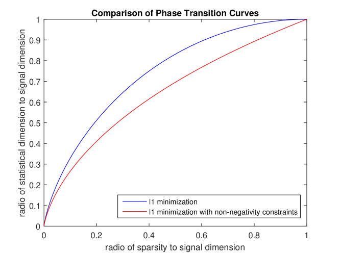
Figure 2: Illustration of the phase transition points for $\ell_{1}$ minimization problem with non-negativity constraints (13) and $\ell_{1}$ minimization problem (16). The blue curve is the curve of $\psi_{1}(\theta)$, which is the phase transition point of problem (16), and the red curve is the curve of $\psi_{2}(\theta)$, which is the phase transition point of problem (13).

Remark 7.

In [3, 4], Donoho and Tanner studied the $\ell_{1}$ minimization problem with non-negativity constraints (13). They proved the existence of weak threshold and strong threshold and showed that at the weak threshold, the probability that problem (13) succeeds jumps from $1$ to $1-\epsilon$, where $\epsilon>0$ is some number. Compared with their results, our results are more precise, i.e., we demonstrate that sharp phase transition exists, and provide an accurate estimate for the phase transition point.

VI Simulation results

In this section, we employ several numerical experiments to verify our theoretical results and our computation recipes. In the experiments, we use CVX Matlab package [19] [20] to solve convex programs.

VI-A Simulation Results for $\ell_{1}$ Minimization with $\ell_{2}$ Norm Constraints

We first design an experiment to verify our results about Recipe 1. More precisely, we design the signal to be sparse and assume that its $\ell_{2}$ norm is know beforehand, and solve problem (9) to recover the signal. The experiment settings are as follows: We set the ambient dimension $n$ to be $128$. The measurement number $m$ increases from $1$ to $128$ with step $1$, and the sparsity level $s$ of the signal increases from $1$ to $128$ with step $1$ as well. For each pair of selections of $m$ and $s$, we generate the true signal $\bm{x}^{\star}$ with $s$ independent standard normal entries and $n-s$ zeros, sample the sensing matrix $\bm{A}$ from the standard normal distribution on $\mathbb{R}^{m\times n}$, and obtain the observation $\bm{y}=\bm{A}\bm{x}^{\star}$. Then we run and solve problem (9) $20$ times. We declare success if the solution $\hat{\bm{x}}$ satisfies $\|\hat{\bm{x}}-\bm{x}^{\star}\|_{2}\leq 10^{-4}$. After all these are done, we calculate the empirical probability of successful recovery. At last, we plot the theoretical curve predicted by Corollary 2.

Moreover, Proposition 2 and Proposition 3 imply that the phase transition point of problem (9) and that of (16) are nearly the same. Therefore, as a comparison, we design an experiment to obtain the empirical probability of successful recovery of problem (16). The experiment settings are absolutely the same as the experiment for problem (9), except that we solve problem (16) for recovery this time.

The simulation results of problems (9) and (16) are presented in Fig. 3(b). Fig. 3(b)(a) shows that the theoretical threshold, predicted by our Corollary 2, matches the empirical phase transition of problem (9) perfectly. Moreover, comparing Fig. 3(b)(a) and Fig. 3(b)(b), we can see that the phase transition points of problem (9) and (16) are almost the same, which verifies our Proposition 2 and Proposition 3. These results imply that our Recipe 1 can provide an accurate estimation of the statistical dimension of the prior restricted cone, when applied to problem (9).

(a) Phase Transition of Problem (9)

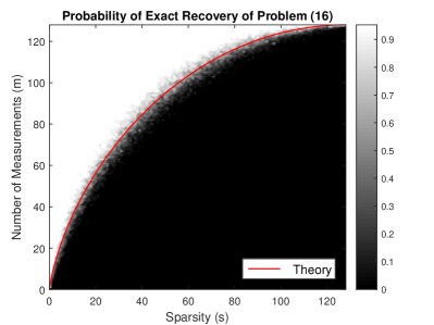
(b) Phase Transition of Problem (16)

Figure 3: Simulation results. In figures (a), (b), we present the simulation results for the phase transition of problems (9) and (16), respectively. In both figures, the gray level represents the empirical probability of successful recovery: Black means failure, and white means success. The red curves plot the phase transition points predicted by our theoretical results in Corollary 2, i.e., either of the red curves denotes the curve of $n\cdot\psi_{1}(s/n)$.

.

VI-B Simulation results for $\ell_{1}$ minimization with non-negativity constraints

The second experiment is designed to verify our results about Recipe 2. More precisely, we design the signal to be non-negative and sparse, and solve problem (13) to recover the signal. The experiment settings are similar as the previous experiment: The ambient dimension $n$ is setted to be $128$, the measurement number $m$ increases from $1$ to $128$ with step $1$, and the sparsity level $s$ of the signal increases from $1$ to $128$ with step $1$. For each pair of selections of $m$ and $s$, we repeat the following process $20$ times. We generate a sparse vector $\tilde{\bm{x}}$ with $s$ independent standard normal entries and $n-s$ zeros, make the true signal $\bm{x}^{\star}_{i}=|\tilde{\bm{x}}_{i}|$ for all $1\leq i\leq n$, sample the sensing matrix $\bm{A}$ from the standard normal distribution on $\mathbb{R}^{m\times n}$, and obtain the observation $\bm{y}=\bm{A}\bm{x}^{\star}$. Then we run and solve problem (13). We declare success if the solution $\hat{\bm{x}}$ to problem (13) satisfies $\|\hat{\bm{x}}-\bm{x}^{\star}\|_{2}\leq 10^{-4}$. After all these are done, we calculate the empirical probability of successful recovery. At last, we plot the theoretical curve predicted by Corollary 4.

Fig. 4 reports our simulation results. It reflects that our theoretical phase transition curve, given by Corollary 4, can predict the empirical phase transition of problem (13) accurately. This implies that our Recipe 2 can provide a reliable estimate of the statistical dimension of the prior restricted cone, when applied to problem (13).

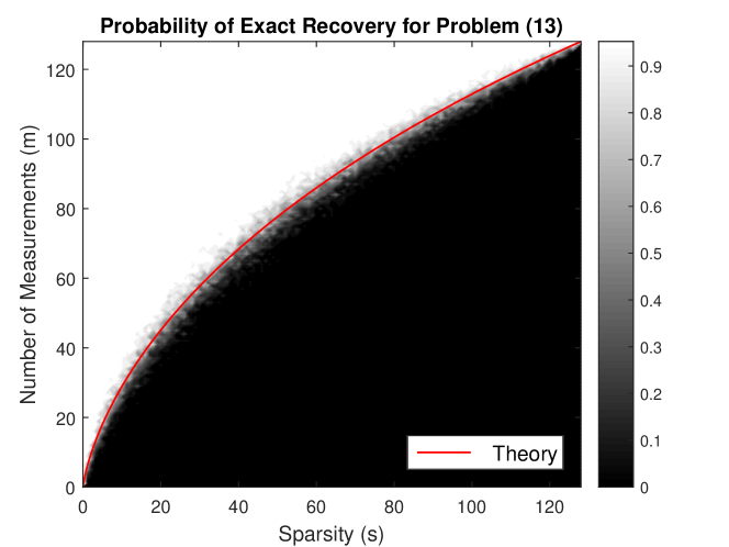
Figure 4: Simulation results for the phase transition of problem (13). In this figure, the gray level represents the empirical probability of successful recovery: Black means failure, and white means success. The red curve plots the phase transition threshold predicted by Corollary 4, i.e., $n\cdot\psi_{2}(s/n)$.

VII Conclusion

This paper studied the phase transition of convex programs with multiple prior constraints, to solve the linear inverse problem. Given such a convex program, we defined its prior restricted set and prior restricted cone, and proved that the phase transition occurs at the statistical dimension of the prior restricted cone. To apply our theoretical results, we presented two recipes, which works under different conditions, to compute the statistical dimension of the prior restricted cone, and a precise analysis of these two recipes were given. Moreover, to illustrate our results, we applied our theoretical results and the estimation recipes to several specific problems, and obtained computable formulas for the statistical dimension and related error bounds. Simulations were provided to demonstrate our results.

Appendix A Proof of Lemma 1

Sufficiency. We argue by contradiction. Suppose that $\mathcal{C}\cap\operatorname{null}(\bm{A})=\{\bm{0}\}$, but problem (2) fails. Then, the solution to problem (2), $\hat{\bm{x}}$, satisfies $\hat{\bm{x}}\neq\bm{x}^{\star}$. Since $\hat{\bm{x}}$ is the solution, $\hat{\bm{x}}$ must have smaller or equal cost than $\bm{x}^{\star}$, and satisfy all the constraints, i.e.,

$$f_{i}(\hat{\bm{x}})\leq f_{i}(\bm{x}^{\star}),\quad\textnormal{for all }0\leq i\leq k,$$ (17)

and

$$\bm{y}=\bm{A}\hat{\bm{x}}.$$ (18)

The identity (17) implies that $\hat{\bm{x}}-\bm{x}^{\star}\in\mathcal{C}$ and the identity (18) implies that $\hat{\bm{x}}-\bm{x}^{\star}\in\operatorname{null}(\bm{A})$. Thus, $\hat{\bm{x}}-\bm{x}^{\star}\in\mathcal{C}\cap\operatorname{null}(\bm{A})$. As $\hat{\bm{x}}\neq\bm{x}^{\star}$, we know that $\mathcal{C}\cap\operatorname{null}(\bm{A})\neq\{\bm{0}\}$. A contradiction.

Necessaty. Again we argue by contradiction. Suppose that problem (2) succeeds, but we have $\mathcal{C}\cap\operatorname{null}(\bm{A})\neq\{\bm{0}\}$. Take any $\bm{d}\in\mathcal{C}\cap\operatorname{null}(\bm{A})$ and $\bm{d}\neq\bm{0}$. Since $\mathcal{C}=\operatorname{cone}(\mathcal{S})$, where $\mathcal{S}$ is the prior restricted set of problem (2), there exists a $t>0$ such that $t\bm{d}\in\mathcal{S}$. The definition of $\mathcal{S}$ implies that

$$f_{i}(\bm{x}^{\star}+t\bm{d})\leq f_{i}(\bm{x}^{\star}),\quad\textnormal{for all }0\leq i\leq k.$$

Moreover, $\bm{d}\in\operatorname{null}(\bm{A})$ implies that

$$\bm{y}=\bm{A}(\bm{x}^{\star}+t\bm{d}).$$

In other words, we have shown that $\bm{x}^{\star}+t\bm{d}$ has smaller or equal cost than $\bm{x}^{\star}$, and satisfies all the constraints. Thus, $\bm{x}^{\star}$ must not be the unique solution to problem (2). A contradiction.

Appendix B Proof of Theorem 2

In this section, we prove our Theorem 2 and related results. In subsection B-A, we prove Lemma 2. In subsections B-B and B-C, we give a detailed a proof of the properties of the function $J$, defined in Theorem 2. The proof idea is inspired by [10, Appendix C], but our proof relies on some different proof techniques. In subsection B-D, we complete the proof for Theorem 2.

B-A Proof of Lemma 2

To begin, note that the prior restricted cone $\mathcal{C}$ is determined by several descent cones of convex functions. Actually, by definition, the prior restricted set $\mathcal{S}$ can be expressed as:

$$\mathcal{S}=D_{s}(f_{0},\bm{x}^{\star})\cap D_{s}(f_{1},\bm{x}^{\star})\cap\dots\cap D_{s}(f_{k},\bm{x}^{\star}),$$

where

$$D_{s}(f_{i},\bm{x}^{\star})=\big{\{}\bm{d}:f_{i}(\bm{x}^{\star}+\bm{d})\leq f_{i}(\bm{x}^{\star})\big{\}}\quad\textnormal{for }i=0,1,\dots,k.$$

Now we argue that

$$\mathcal{C}=D(f_{0},\bm{x}^{\star})\cap D(f_{1},\bm{x}^{\star})\cap\dots\cap D(f_{k},\bm{x}^{\star}),$$ (19)

where $D(f_{i},\bm{x}^{\star})$ denotes the descent cones of $f_{i}$ at $\bm{x}^{\star}$, $i=0,1,\dots,k$, i.e.,

$$D(f_{i},\bm{x}^{\star})=\operatorname{cone}\big{(}D_{s}(f_{i},\bm{x}^{\star})\big{)}=\big{\{}\bm{d}:\exists\,t>0,f_{i}(\bm{x}^{\star}+t\bm{d})\leq f_{i}(\bm{x}^{\star})\big{\}}\quad\textnormal{for }i=0,1,\dots,k.$$

To see this, first note that it is clear that $\mathcal{C}\subseteq D(f_{0},\bm{x}^{\star})\cap D(f_{1},\bm{x}^{\star})\cap\dots\cap D(f_{k},\bm{x}^{\star})$, so it remains to show the reverse relation holds. Take any $\bm{d}\in D(f_{0},\bm{x}^{\star})\cap D(f_{1},\bm{x}^{\star})\cap\dots\cap D(f_{k},\bm{x}^{\star})$, then there exists some number $t_{i}>0$ such that $t_{i}\bm{d}\in D_{s}(f_{i},\bm{x}^{\star})$ for any $0\leq i\leq k$. Denote $t\coloneqq\min_{0\leq i\leq k}t_{i}>0$. The convexity of $f_{i}$ implies that

$$f_{i}(\bm{x}^{\star}+t\bm{d})=f_{i}\big{(}(1-\lambda_{i})\bm{x}^{\star}+\lambda_{i}(\bm{x}^{\star}+t_{i}\bm{d})\big{)}\leq(1-\lambda_{i})f_{i}(\bm{x}^{\star})+\lambda_{i}f_{i}(\bm{x}^{\star}+t_{i}\bm{d})\leq f_{i}(\bm{x}^{\star}),$$

where $\lambda_{i}=t/t_{i}\in(0,1]$. Since the above inequality holds for any $0\leq i\leq k$, we obtain that $t\bm{d}\in\mathcal{S}$. Thus, $\bm{d}\in\mathcal{C}$. The identity (19) follows immediately.

Next, taking polar on both sides of (19) yields

$$\mathcal{C}^{\circ}=\big{[}D(f_{0},\bm{x}^{\star})\cap D(f_{1},\bm{x}^{\star})\cap\dots\cap D(f_{k},\bm{x}^{\star})\big{]}^{\circ}.$$

Since we have assumed that $\operatorname{ri}\big{(}D(f_{0},\bm{x}^{\star})\big{)}\cap\operatorname{ri}\big{(}D(f_{1},\bm{x}^{\star})\big{)}\cap\dots\cap\operatorname{ri}\big{(}D(f_{k},\bm{x}^{\star})\big{)}\neq\emptyset$, by [17, Corollary 23.8.1], the normal cone to the intersection of sets is the Minkowski sum of the normal cones to the individual sets:

$$\mathcal{C}^{\circ}=\big{[}D(f_{0},\bm{x}^{\star})\cap D(f_{1},\bm{x}^{\star})\cap\dots\cap D(f_{k},\bm{x}^{\star})\big{]}^{\circ}=\sum_{i=0}^{k}N(f_{i},\bm{x}^{\star}).$$ (20)

Recall that the statistical dimension of a convex cone can be expressed via its polar [10, Proposition 3.1 (4)], so we obtain from (20) that

$$\delta(\mathcal{C})=\mathbb{E}\big{[}\operatorname{dist}^{2}(\bm{g},\mathcal{C}^{\circ})\big{]}=\mathbb{E}\big{[}\operatorname{dist}^{2}(\bm{g},\sum_{i=0}^{k}N(f_{i},\bm{x}^{\star}))\big{]}.$$

B-B Distance to the Sum of Compact Sets

In this subsection, we study some analytic properties of the function $J_{\bm{u}}(\bm{\tau})$, which is related to $J(\bm{\tau})$, but more simpler. We begin by studying some properties of the Minkowski sum of compact sets.

Lemma 3 (Sum of compact sets).

For any $0\leq i\leq k$, let $S_{i}$ be a non-empty, compact, convex subset of $\mathbb{R}^{n}$ that does not contain the origin, and $\bm{\tau}\in\mathbb{S}^{k}\cap\mathbb{R}^{k+1}_{+}$. Suppose that $\|\bm{s}_{i}\|_{2}\leq B_{i}$ for some $B_{i}>0$ and for any $\bm{s}_{i}\in S_{i}$, $0\leq i\leq k$. Then there exists a number $B>0$ such that

$$\Big{\|}\sum_{i=0}^{k}\bm{\tau}_{i}\bm{s}_{i}\Big{\|}_{2}\leq B,\ \textnormal{for any }\bm{\tau}\in\mathbb{S}^{k}\cap\mathbb{R}^{k+1}_{+}\ \textnormal{and}\ \bm{s}_{i}\in S_{i},\ 0\leq i\leq k.$$ (21)

Furthermore, suppose that

$$\bm{0}\notin\sum_{i=0}^{k}\bm{\tau}_{i}S_{i},\ \textnormal{for any }\bm{\tau}\in\mathbb{S}^{k}\cap\mathbb{R}^{k+1}_{+}.$$

Then there exists a number $b>0$ such that

$$\Big{\|}\sum_{i=0}^{k}\bm{\tau}_{i}\bm{s}_{i}\Big{\|}_{2}\geq b,\ \textnormal{for any }\bm{\tau}\in\mathbb{S}^{k}\cap\mathbb{R}^{k+1}_{+},\ \textnormal{and}\ \bm{s}_{i}\in S_{i},\ 0\leq i\leq k.$$ (22)

Proof.

Upper bound. The upper bound in (21) is easy to obtain. Actually, by the triangle inequality and the Cauchy-Schwarz inequality, for any $\bm{\tau}\in\mathbb{S}^{q}\cap\mathbb{R}^{q+1}_{+}$, we have

$$\Big{\|}\sum_{i=0}^{k}\bm{\tau}_{i}\bm{s}_{i}\Big{\|}_{2}\leq\sum_{i=0}^{k}\bm{\tau}_{i}\|\bm{s}_{i}\|_{2}\leq\|\bm{\tau}\|_{2}\cdot\sqrt{\sum_{i=0}^{k}\|\bm{s}_{i}\|_{2}^{2}}\leq\|\bm{\tau}\|_{2}\cdot\sqrt{\sum_{i=0}^{k}B_{i}^{2}}=\sqrt{\sum_{i=0}^{k}B_{i}^{2}}\coloneqq B.$$

Lower bound. We prove the lower bound by contradiction. Suppose that there does not exist $b>0$ satisfying (22), which implies that

$$\inf_{\bm{\tau}\in\mathbb{S}^{k}\cap\mathbb{R}^{k+1}_{+}}\inf_{\bm{s}_{i}\in S_{i},0\leq i\leq k}\Big{\|}\sum_{i=0}^{k}\bm{\tau}_{i}\bm{s}_{i}\Big{\|}_{2}=0.$$ (23)

Let’s consider the function $r(\bm{\tau})\coloneqq\inf_{\bm{s}_{i}\in S_{i},0\leq i\leq k}\big{\|}\sum_{i=0}^{k}\bm{\tau}_{i}\bm{s}_{i}\big{\|}_{2}$, where $\bm{\tau}\in\mathbb{R}^{k+1}_{+}$, and prove that it is continuous. To this end, let $\bm{\tau},\tilde{\bm{\tau}}\in\mathbb{R}^{k+1}_{+}$. Note that the sum of compact sets is compact [21, Excercise 3(d), page 38]. As a result, both $\sum_{i=0}^{k}\bm{\tau}_{i}S_{i}$ and $\sum_{i=0}^{k}\tilde{\bm{\tau}}_{i}S_{i}$ are compact. It follows that there exists $\bm{s}_{i}^{\star}\in S_{i}$, $0\leq i\leq k$, such that

$$\Big{\|}\sum_{i=0}^{q}\tilde{\bm{\tau}}_{i}\bm{s}_{i}^{\star}\Big{\|}_{2}=r(\tilde{\bm{\tau}}).$$

Therefore, by the triangle inequality, we have

$$r(\bm{\tau})-r(\tilde{\bm{\tau}}) \leq\Big{\|}\sum_{i=0}^{k}\bm{\tau}_{i}\bm{s}_{i}^{\star}\Big{\|}_{2}-\Big{\|}\sum_{i=0}^{k}\tilde{\bm{\tau}}_{i}\bm{s}_{i}^{\star}\Big{\|}_{2}\leq\Big{\|}\Big{(}\sum_{i=0}^{k}\bm{\tau}_{i}\bm{s}_{i}^{\star}\Big{)}-\Big{(}\sum_{i=0}^{k}\tilde{\bm{\tau}}_{i}\bm{s}_{i}^{\star}\Big{)}\Big{\|}_{2}$$

$$=\Big{\|}\sum_{i=0}^{k}(\bm{\tau}_{i}-\tilde{\bm{\tau}}_{i})\bm{s}_{i}^{\star}\Big{\|}_{2}\leq\|\bm{\tau}-\tilde{\bm{\tau}}\|_{2}\cdot B.$$ (24)

In the last inequality, we have used the upper bound (21). By interchanging the roles of $\bm{\tau}$ and $\tilde{\bm{\tau}}$ in (B-B), we obtain that

$$\big{|}r(\bm{\tau})-r(\tilde{\bm{\tau}})\big{|}\leq\|\bm{\tau}-\tilde{\bm{\tau}}\|_{2}\cdot B,$$ (25)

which implies that $r(\bm{\tau})$ is Lipschitz function. The continuity of $r(\bm{\tau})$ follows immediately. Now recall that a continuous function in a compact set must attain its infimum [22, Theorem 4.16], therefore, (23) indicates that there exists a $\bm{\tau}\in\mathbb{S}^{k}\cap\mathbb{R}^{k+1}_{+}$ such that

$$\inf_{\bm{s}_{i}\in S_{i},0\leq i\leq k}\Big{\|}\sum_{i=0}^{k}\bm{\tau}_{i}\bm{s}_{i}\Big{\|}_{2}=0.$$ (26)

Since $\sum_{i=0}^{k}\bm{\tau}_{i}S_{i}$ is closed, (26) implies that $\bm{0}\in\sum_{i=0}^{k}\bm{\tau}_{i}S_{i}$. A contradiction. Therefore, there must exist some $b>0$ satisfying (22). ∎

Lemma 3 gives upper and lower bounds for the length of elements of sum of compact sets. We remind that when we write $B$ and $b$ hereafter, we always mean the numbers in (21) and (22), respectively. Using Lemma 3, we can study the properties of function $J_{\bm{u}}$, which is the distance of a point to sum of compact sets.

Lemma 4 (Distance to the sum of compact sets).

Let $S_{i}$, $0\leq i\leq k$, be a non-empty, compact, convex subset of $\mathbb{R}^{n}$ that does not contain the origin. Suppose that $\|\bm{s}_{i}\|_{2}\leq B_{i}$ for some $B_{i}>0$ and for any $\bm{s}_{i}\in S_{i}$, $0\leq i\leq k$. Moreover, suppose that

$$\bm{0}\notin\sum_{i=0}^{k}\bm{\tau}_{i}S_{i},\ \ \textnormal{for any }\bm{\tau}\in\mathbb{S}^{k}\cap\mathbb{R}^{k+1}_{+}.$$ (27)

Fix a point $\bm{u}\in\mathbb{R}^{n}$, and define the function $J_{\bm{u}}:\mathbb{R}_{+}^{k+1}\rightarrow\mathbb{R}$ by

$$J_{\bm{u}}(\bm{\tau})\coloneqq\operatorname{dist}^{2}(\bm{u},\sum_{i=0}^{k}\bm{\tau}_{i}S_{i}),$$

where $\bm{\tau}=(\bm{\tau}_{0},\bm{\tau}_{1},\dots,\bm{\tau}_{k})\in\mathbb{R}_{+}^{k+1}$. Then $J_{\bm{u}}(\bm{\tau})$ has the following properties:

1. The function $J_{\bm{u}}$ is convex and continuous.

2. The function $J_{\bm{u}}$ has the lower bound

   $$J_{\bm{u}}(\bm{\tau})\geq(\|\bm{\tau}\|_{2}b-\|\bm{u}\|_{2})^{2},\ \textnormal{when }\|\bm{\tau}\|_{2}\geq\frac{\|\bm{u}\|_{2}}{b}.$$ (28)

   In particular, $J_{\bm{u}}$ attains its minimum in the compact subset $\mathbb{B}(\bm{0},2\|\bm{u}\|_{2}/b)\cap\mathbb{R}^{k+1}_{+}$.

3. The function $J_{\bm{u}}$ is continuously differentiable, and its partial derivative is

   $$\frac{\partial J_{\bm{u}}}{\partial\bm{\tau}_{i}}(\bm{\tau})=-2\left<\bm{u}-\sum_{i=0}^{k}\bm{\tau}_{i}\bar{\bm{s}}_{i},\bar{\bm{s}}_{i}\right>\quad\textnormal{for any}\ \bm{\tau}\in\mathbb{R}^{k+1}_{+},$$ (29)

   where $\bar{\bm{s}}_{i}\in S_{i},\,0\leq i\leq k$, satisfies $\operatorname{dist}^{2}(\bm{u},\sum_{i=0}^{k}\bm{\tau}_{i}\bar{\bm{s}}_{i})=J_{\bm{u}}(\bm{\tau})$. For $\bm{\tau}$ in the boundary of $\mathbb{R}^{k+1}_{+}$, we interpret the partial derivative $\frac{\partial J_{\bm{u}}}{\partial\bm{\tau}_{i}}$ similarly as the right derivative if $\bm{\tau}_{i}=0$, i.e.,

   $$\frac{\partial J_{\bm{u}}}{\partial\bm{\tau}_{i}}(\bm{\tau})=\lim_{\epsilon\downarrow 0}\frac{J_{\bm{u}}(\bm{\tau}_{0},\dots,\bm{\tau}_{i-1},\epsilon,\dots,\bm{\tau}_{k})-J_{\bm{u}}(\bm{\tau}_{0},\dots,\bm{\tau}_{i-1},0,\dots,\bm{\tau}_{k})}{\epsilon}.$$

4. The partial derivative of $J_{\bm{u}}$ satisfies the following bound:

   $$\Big{|}\frac{\partial J_{\bm{u}}}{\partial\bm{\tau}_{i}}(\bm{\tau})\Big{|}\leq 2B_{i}\big{(}\|\bm{u}\|_{2}+\|\bm{\tau}\|_{2}B\big{)}.$$ (30)

5. For any fixed $\bm{\tau}\in\mathbb{R}^{k+1}_{+}$ and any $0\leq i\leq k$, the map $\bm{u}\mapsto\frac{\partial J_{\bm{u}}}{\partial\bm{\tau}_{i}}(\bm{\tau})$ is Lipschitz:

   $$\Big{|}\frac{\partial J_{\bm{u}}}{\partial\bm{\tau}_{i}}(\bm{\tau})-\frac{\partial J_{\bm{u}^{\prime}}}{\partial\bm{\tau}_{i}}(\bm{\tau})\Big{|}\leq 2B_{i}\cdot\|\bm{u}-\bm{u}^{\prime}\|_{2}.$$ (31)

Proof.

Lemma 4 is a generalization of [10, Lemma C.1] from a dilated set to the sum of several sets.

Convexity. Note that to prove the convexity of $J_{\bm{u}}$, it is sufficient to prove that the function

$$J^{\frac{1}{2}}_{\bm{u}}(\bm{\tau})\coloneqq\sqrt{J_{\bm{u}}(\bm{\tau})}=\operatorname{dist}(\bm{u},\sum_{i=0}^{k}\bm{\tau}_{i}S_{i})$$

is convex. To this end, fix any $\bm{\tau},\tilde{\bm{\tau}}\in\mathbb{R}^{k+1}_{+}$ and $\lambda_{1},\lambda_{2}\in\mathbb{R}_{+}$ satisfying $\lambda_{1}+\lambda_{2}=1$. Since $S_{i}$ is a convex set for $0\leq i\leq k$, it follows from [17, Theorem 3.2] that

$$(\lambda_{1}\bm{\tau}_{i}+\lambda_{2}\tilde{\bm{\tau}}_{i})S_{i}=\lambda_{1}\bm{\tau}_{i}S_{i}+\lambda_{2}\tilde{\bm{\tau}}_{i}S_{i}\ \ \textnormal{for any}\ \ 0\leq i\leq k.$$ (32)

Then by the definition of $J_{\bm{u}}^{\frac{1}{2}}$ and the triangle inequality, we have

$$J^{\frac{1}{2}}_{\bm{u}}(\lambda_{1}\bm{\tau}+\lambda_{2}\tilde{\bm{\tau}}) =\operatorname{dist}\big{(}\bm{u},\sum_{i=0}^{k}(\lambda_{1}\bm{\tau}_{i}+\lambda_{2}\tilde{\bm{\tau}}_{i})S_{i}\big{)}=\operatorname{dist}\big{(}\bm{u},\sum_{i=0}^{k}(\lambda_{1}\bm{\tau}_{i}S_{i}+\lambda_{2}\tilde{\bm{\tau}}_{i}S_{i})\big{)}$$

$$=\operatorname{dist}\big{(}\lambda_{1}\bm{u}+\lambda_{2}\bm{u},\lambda_{1}(\sum_{i=0}^{k}\bm{\tau}_{i}S_{i})+\lambda_{2}(\sum_{i=0}^{k}\tilde{\bm{\tau}}_{i}S_{i})\big{)}$$

$$=\inf_{\bm{s}_{i}\in S_{i},\tilde{\bm{s}}_{i}\in S_{i},0\leq i\leq k}\Big{\|}\lambda_{1}\bm{u}+\lambda_{2}\bm{u}-\big{[}\lambda_{1}\cdot\big{(}\sum_{i=0}^{k}\bm{\tau}_{i}\bm{s}_{i}\big{)}+\lambda_{2}\cdot\big{(}\sum_{i=0}^{k}\tilde{\bm{\tau}}_{i}\tilde{\bm{s}}_{i}\big{)}\big{]}\Big{\|}_{2}$$

$$\leq\inf_{\bm{s}_{i}\in S_{i},\tilde{\bm{s}}_{i}\in S_{i},0\leq i\leq k}\lambda_{1}\Big{\|}\bm{u}-\sum_{i=0}^{k}\bm{\tau}_{i}\bm{s}_{i}\Big{\|}_{2}+\lambda_{2}\Big{\|}\bm{u}-\sum_{i=0}^{k}\tilde{\bm{\tau}}_{i}\tilde{\bm{s}}_{i}\Big{\|}_{2}$$

$$=\lambda_{1}\cdot\operatorname{dist}\big{(}\bm{u},\sum_{i=0}^{k}\bm{\tau}_{i}S_{i}\big{)}+\lambda_{2}\cdot\operatorname{dist}\big{(}\bm{u},\sum_{i=0}^{k}\tilde{\bm{\tau}}_{i}S_{i}\big{)}$$

$$=\lambda_{1}J^{\frac{1}{2}}_{\bm{u}}(\bm{\tau})+\lambda_{2}J^{\frac{1}{2}}_{\bm{u}}(\tilde{\bm{\tau}}),$$

which implies that $J^{\frac{1}{2}}_{\bm{u}}$ is convex. The convexity of $J_{\bm{u}}$ follows immediately.

Continiuty. We first consider the case when $\bm{\tau}\in\mathbb{R}^{k+1}_{++}$ and take any $\bm{\epsilon}\in\mathbb{R}^{k+1}$. To check the continuity, note that

$$J^{\frac{1}{2}}_{\bm{u}}(\bm{\tau}+\bm{\epsilon})=\operatorname{dist}\Big{(}\bm{u},\sum_{i=0}^{k}(\bm{\tau}_{i}+\bm{\epsilon}_{i})S_{i}\Big{)}=\inf_{\bm{s}_{i}\in S_{i},0\leq i\leq k}\Big{\|}\bm{u}-\big{(}\sum_{i=0}^{k}\bm{\epsilon}_{i}\bm{s}_{i}+\sum_{i=0}^{k}\bm{\tau}_{i}\bm{s}_{i}\big{)}\Big{\|}_{2}.$$ (33)

The triangle inequality gives us that

$$\Big{\|}\bm{u}-\sum_{i=0}^{k}\bm{\tau}_{i}\bm{s}_{i}\Big{\|}_{2}-\Big{\|}\sum_{i=0}^{k}\bm{\epsilon}_{i}\bm{s}_{i}\Big{\|}_{2}\leq\Big{\|}\bm{u}-\big{(}\sum_{i=0}^{k}\bm{\epsilon}_{i}\bm{s}_{i}+\sum_{i=0}^{k}\bm{\tau}_{i}\bm{s}_{i}\big{)}\Big{\|}_{2}\leq\Big{\|}\bm{u}-\sum_{i=0}^{k}\bm{\tau}_{i}\bm{s}_{i}\Big{\|}_{2}+\Big{\|}\sum_{i=0}^{k}\bm{\epsilon}_{i}\bm{s}_{i}\Big{\|}_{2}.$$ (34)

Putting (33) and (34) together, we obtain that

$$\operatorname{dist}\Big{(}\bm{u},\sum_{i=0}^{k}\bm{\tau}_{i}S_{i}\Big{)}-\sup_{\bm{s}_{i}\in S_{i},\atop 0\leq i\leq k}\Big{\|}\sum_{i=0}^{k}\bm{\epsilon}_{i}\bm{s}_{i}\Big{\|}_{2}\leq\operatorname{dist}\Big{(}\bm{u},\sum_{i=0}^{k}(\bm{\tau}_{i}+\bm{\epsilon}_{i})S_{i}\Big{)}\leq\operatorname{dist}\Big{(}\bm{u},\sum_{i=0}^{k}\bm{\tau}_{i}S_{i}\Big{)}+\sup_{\bm{s}_{i}\in S_{i},\atop 0\leq i\leq k}\Big{\|}\sum_{i=0}^{k}\bm{\epsilon}_{i}\bm{s}_{i}\Big{\|}_{2}.$$ (35)

Now recalling the upper bound in (21), we obtain from (35) that

$$\operatorname{dist}\Big{(}\bm{u},\sum_{i=0}^{k}\bm{\tau}_{i}S_{i}\Big{)}-\|\bm{\epsilon}\|_{2}B\leq\operatorname{dist}\Big{(}\bm{u},\sum_{i=0}^{k}(\bm{\tau}_{i}+\bm{\epsilon}_{i})S_{i}\Big{)}\leq\operatorname{dist}\Big{(}\bm{u},\sum_{i=0}^{k}\bm{\tau}_{i}S_{i}\Big{)}+\|\bm{\epsilon}\|_{2}B.$$

In other words,

$$J^{\frac{1}{2}}_{\bm{u}}(\bm{\tau})-\|\bm{\epsilon}\|_{2}B\leq J^{\frac{1}{2}}_{\bm{u}}(\bm{\tau}+\bm{\epsilon})\leq J^{\frac{1}{2}}_{\bm{u}}(\bm{\tau})+\|\bm{\epsilon}\|_{2}B.$$ (36)

Squaring both sides, we obtain that

$$\|\bm{\epsilon}\|^{2}_{2}B^{2}-2\|\bm{\epsilon}\|_{2}B\cdot J^{\frac{1}{2}}_{\bm{u}}(\bm{\tau})\leq J_{\bm{u}}(\bm{\tau}+\bm{\epsilon})-J_{\bm{u}}(\bm{\epsilon})\leq\|\bm{\epsilon}\|_{2}^{2}B^{2}+2\|\bm{\epsilon}\|_{2}B\cdot J_{\bm{u}}^{\frac{1}{2}}(\bm{\tau}).$$

Moreover, select any $\bm{s}_{i}\in S_{i}$, $0\leq i\leq k$, and we have

$$J_{\bm{u}}^{\frac{1}{2}}(\bm{\tau})=\operatorname{dist}(\bm{u},\sum_{i=0}^{k}\bm{\tau}_{i}S_{i})\leq\|\bm{u}-\sum_{i=0}^{k}\bm{\tau}_{i}\bm{s}_{i}\|_{2}\leq\|\bm{u}\|_{2}+\big{\|}\sum_{i=0}^{k}\bm{\tau}_{i}\bm{s}_{i}\big{\|}_{2}\leq\|\bm{u}\|_{2}+\|\bm{\tau}\|_{2}B,$$

where we have used the triangle inequality and the upper bound (21). It follows that

$$\big{|}J_{\bm{u}}(\bm{\tau}+\bm{\epsilon})-J_{\bm{u}}(\bm{\epsilon})\big{|} \leq\|\bm{\epsilon}\|_{2}^{2}B^{2}+2\|\bm{\epsilon}\|_{2}B\cdot J_{\bm{u}}^{\frac{1}{2}}(\bm{\tau})=\|\bm{\epsilon}\|_{2}^{2}B^{2}+2\|\bm{\epsilon}\|_{2}B\cdot\operatorname{dist}(\bm{u},\sum_{i=0}^{k}\bm{\tau}_{i}S_{i})$$

$$\leq\|\bm{\epsilon}\|_{2}^{2}B^{2}+2\|\bm{\epsilon}\|_{2}B\cdot\big{(}\|\bm{u}\|_{2}+\|\bm{\tau}\|_{2}B\big{)}.$$ (37)

Now it is easy to see that if $\epsilon\rightarrow\bm{0}$, we have $\big{|}J_{\bm{u}}(\bm{\tau}+\bm{\epsilon})-J_{\bm{u}}(\bm{\epsilon})\big{|}\rightarrow 0$. Similar argument holds as well when $\bm{\tau}$ is on the boundary of $\mathbb{R}_{+}^{k+1}$. Therefore, we conclude that the function $J_{\bm{u}}$ is continuous in $\mathbb{R}_{+}^{k+1}$.

Attainment of minimum. Note that by Lemma 3, we know that there exists a number $b>0$ such that

$$\Big{\|}\sum_{i=0}^{k}\bm{\tau}_{i}\bm{s}_{i}\Big{\|}_{2}\geq b,\ \textnormal{for any }\bm{\tau}\in\mathbb{S}^{k}\cap\mathbb{R}^{k+1}_{+},\ \bm{s}_{i}\in S_{i},\ 0\leq i\leq k.$$

Therefore, for any $\bm{\tau}\neq\bm{0}$,

$$J^{\frac{1}{2}}_{\bm{u}}(\bm{\tau})=\operatorname{dist}(\bm{u},\sum_{i=0}^{k}\bm{\tau}_{i}S_{i})=\inf_{\bm{s}_{i}\in S_{i},0\leq i\leq k}\big{\|}\bm{u}-\sum_{i=0}^{k}\bm{\tau}_{i}\bm{s}_{i}\big{\|}_{2}\geq\inf_{\bm{s}_{i}\in S_{i},0\leq i\leq k}\big{\|}\sum_{i=0}^{k}\bm{\tau}_{i}\bm{s}_{i}\big{\|}_{2}-\|\bm{u}\|_{2}\geq\|\bm{\tau}\|_{2}\cdot b-\|\bm{u}\|_{2}.$$ (38)

Thus, when $\|\bm{\tau}\|_{2}\geq\|\bm{u}\|_{2}/b$, by squaring both sides of (38), we obtain the lower bound

$$J_{\bm{u}}(\bm{\tau})\geq\big{(}\|\bm{\tau}\|_{2}\cdot b-\|\bm{u}\|_{2}\big{)}^{2}.$$

Moreover, if $\|\bm{\tau}\|_{2}\geq 2\|\bm{u}\|_{2}/b$, we have $J_{\bm{u}}(\bm{\tau})\geq\|\bm{u}\|_{2}^{2}=J_{\bm{u}}(\bm{0})$. Then, it follows from the convexity and continuity of $J_{\bm{u}}$ that the function $J_{\bm{u}}$ must attain its minimum in the compact set $\mathbb{B}(\bm{0},2\|\bm{u}\|_{2}/b)\cap\mathbb{R}^{k+1}_{+}$.

Continuous differentiability in $\mathbb{R}^{k+1}_{++}$. To prove that $J_{\bm{u}}$ is continuously differential in $\mathbb{R}^{k+1}_{++}$, we need to show that the partial derivative $\partial J_{\bm{u}}/\partial\bm{\tau}_{i}$ exists and is continuous, for any $0\leq i\leq k$. For this purpose, fix any $0\leq i\leq k$, and define the function $\tilde{J}_{\bm{u}}(\bm{\tau}_{i})$ to be

$$\tilde{J}_{\bm{u}}(\bm{\tau}_{i})\coloneqq J_{\bm{u}}(\bm{\tau})=\operatorname{dist}^{2}(\bm{u},\sum_{i=0}^{k}\bm{\tau}_{i}S_{i})=\operatorname{dist}^{2}(\bm{u},T+\bm{\tau}_{i}S_{i})=\inf_{\bm{t}\in T}\operatorname{dist}^{2}(\bm{u}-\bm{t},\bm{\tau}_{i}S_{i}),$$ (39)

where $T=\sum_{0\leq j\leq k,j\neq i}\bm{\tau}_{i}S_{i}$. Now define another function $g(\bm{\tau}_{i},\bm{t})=\operatorname{dist}^{2}(\bm{u}-\bm{t},\bm{\tau}_{i}S_{i})$, $(\bm{\tau}_{i},\bm{t})\in\mathbb{R}_{++}\times\mathbb{R}^{n}$. The function $g(\bm{\tau}_{i},\bm{t})$ is continuously differentiable. To see this, first note that the function $\partial g/\partial\bm{\tau}_{i}$ exists, and takes the form

$$\frac{\partial g}{\partial\bm{\tau}_{i}}=-\frac{2}{\bm{\tau}_{i}}\left<\bm{u}-\bm{t}-\Pi_{\bm{\tau}_{i}S_{i}}(\bm{u}-\bm{t}),\Pi_{\bm{\tau}_{i}S_{i}}(\bm{u}-\bm{t})\right>.$$

Moreover, $\partial g/\partial\bm{\tau}_{i}$ is continuous [10, Lemma C.1, (3)]. Next, the function $\tilde{g}(\bm{t})=\operatorname{dist}^{2}(\bm{u}-\bm{t},\bm{\tau}_{i}S_{i})$ is differentiable, and the differential is

$$\nabla\tilde{g}(\bm{t})=-2\big{(}\bm{u}-\bm{t}-\Pi_{\bm{\tau}_{i}S_{i}}(\bm{u}-\bm{t})\big{)}.$$

This point results from [23, Theorem 2.26]. Furthermore, the projection onto a convex set is continuous [23, Theorem 2.26], hence, $\nabla\tilde{g}$ is a continuous function. It follows that $\partial g/\partial\bm{t}_{j}$ is continuous for any $1\leq j\leq n$. Therefore, we obtain that the function $g(\bm{\tau}_{i},\bm{t})$ is continuously differentiable in $\mathbb{R}_{++}\times\mathbb{R}^{n}$. As a result of [24, Theorem 2.8], $g(\bm{\tau}_{i},\bm{t})$ is differentiable in $\mathbb{R}_{++}\times\mathbb{R}^{n}$, and the differential is

$$\nabla g(\bm{\tau}_{i},\bm{t})=\Big{[}-\frac{2}{\bm{\tau}_{i}}\left<\bm{u}-\bm{t}-\Pi_{\bm{\tau}_{i}S_{i}}(\bm{u}-\bm{t}),\Pi_{\bm{\tau}_{i}S_{i}}(\bm{u}-\bm{t})\right>,-2\big{(}\bm{u}-\bm{t}-\Pi_{\bm{\tau}_{i}S_{i}}(\bm{u}-\bm{t})\big{)}^{T}\Big{]}^{T}.$$

The subdifferential of a differentiable function contains only the differential of the function [17, Theorem 25.1]. Thus, the subdifferential of $g$ at $(\bm{\tau}_{i},\bm{t})$ is

$$\partial g(\bm{\tau}_{i},\bm{t})=\Big{\{}\Big{[}-\frac{2}{\bm{\tau}_{i}}\left<\bm{u}-\bm{t}-\Pi_{\bm{\tau}_{i}S_{i}}(\bm{u}-\bm{t}),\Pi_{\bm{\tau}_{i}S_{i}}(\bm{u}-\bm{t})\right>,-2\big{(}\bm{u}-\bm{t}-\Pi_{\bm{\tau}_{i}S_{i}}(\bm{u}-\bm{t})\big{)}^{T}\Big{]}^{T}\Big{\}}.$$ (40)

Since $T$ is compact, we can take a $\bar{\bm{t}}\in T$ such that $g(\bm{\tau}_{i},\bar{\bm{t}})=\tilde{J}_{\bm{u}}(\bm{\tau}_{i})$. Then let us confirm that $-\nabla\tilde{g}(\bar{\bm{t}})=2\big{(}\bm{u}-\bar{\bm{t}}-\Pi_{\bm{\tau}_{i}S_{i}}(\bm{u}-\bar{\bm{t}})\big{)}\in N(\bar{\bm{t}};T)$, where $N(\bar{\bm{t}};T)\coloneqq\{\bm{w}\in\mathbb{R}^{n}:\left<\bm{w},\bm{t}-\bar{\bm{t}}\right>\leq 0,\ \forall\,\bm{t}\in T\}$, denotes the normal cone to $T$ at $\bar{\bm{t}}$. To this end, let $\bm{s}_{i}\in S_{i}$ such that $\bm{\tau}_{i}\bm{s}_{i}=\Pi_{\bm{\tau}_{i}S_{i}}(\bm{u}-\bar{\bm{t}})$. From another point of view, it is not difficult to see that $\bar{\bm{t}}=\Pi_{T}(\bm{u}-\bm{\tau}_{i}\bm{s}_{i})$. Thus,

$$-\nabla\tilde{g}(\bar{\bm{t}})=2\big{(}\bm{u}-\bar{\bm{t}}-\Pi_{\bm{\tau}_{i}S_{i}}(\bm{u}-\bar{\bm{t}})\big{)}=2\big{(}\bm{u}-\bm{\tau}_{i}\bm{s}_{i}-\Pi_{T}(\bm{u}-\bm{\tau}_{i}\bm{s}_{i})\big{)}.$$

By [25, Theorem III.3.1.1], we know that

$$\left<\bm{u}-\bm{\tau}_{i}\bm{s}_{i}-\Pi_{T}(\bm{u}-\bm{\tau}_{i}\bm{s}_{i}),\bm{t}-\Pi_{T}(\bm{u}-\bm{\tau}_{i}\bm{s}_{i})\right>\leq 0,\ \textnormal{for any}\ \bm{t}\in T.$$

Therefore, we obtain that

$$-\nabla\tilde{g}(\bar{\bm{t}})=2\big{(}\bm{u}-\bar{\bm{t}}-\Pi_{\bm{\tau}_{i}S_{i}}(\bm{u}-\bar{\bm{t}})\big{)}\in N(\bar{\bm{t}};T).$$ (41)

Now we can give a conclusion about the subdifferential of $\tilde{J}_{\bm{u}}$:

$$\partial\tilde{J}_{\bm{u}}(\bm{\tau}_{i})=\Big{\{}-\frac{2}{\bm{\tau}_{i}}\left<\bm{u}-\bar{\bm{t}}-\Pi_{\bm{\tau}_{i}S_{i}}(\bm{u}-\bar{\bm{t}}),\Pi_{\bm{\tau}_{i}S_{i}}(\bm{u}-\bar{\bm{t}})\right>\Big{\}}.$$

This is a direct consequence of [18, Example 2.59 and Theorem 2.61], (40), (41), and the fact that $g(\bm{\tau}_{i},\bm{t})$ is continuous. That the subdifferential of $\tilde{J}_{\bm{u}}$ is a singleton implies $\tilde{J}_{\bm{u}}$ is differentiable [17, Theorem 25.1], and the differential is

$$\tilde{J}^{\prime}_{\bm{u}}(\bm{\tau}_{i})=-\frac{2}{\bm{\tau}_{i}}\left<\bm{u}-\bar{\bm{t}}-\Pi_{\bm{\tau}_{i}S_{i}}(\bm{u}-\bar{\bm{t}}),\Pi_{\bm{\tau}_{i}S_{i}}(\bm{u}-\bar{\bm{t}^{\prime}})\right>.$$

The above formula is equivalent to that the partial derivative $\partial J_{\bm{u}}/\partial\bm{\tau}_{i}$ exists, and takes the form

$$\frac{\partial J_{\bm{u}}}{\partial\bm{\tau}_{i}}(\bm{\tau})=-\frac{2}{\bm{\tau}_{i}}\left<\bm{u}-\bar{\bm{t}}-\bm{\tau}_{i}\bar{\bm{s}}_{i},\bm{\tau}_{i}\bar{\bm{s}}_{i}\right>,$$

for any $\bar{\bm{t}}\in T,\bar{\bm{s}}_{i}\in S_{i}$ such that $\operatorname{dist}^{2}(\bm{u},\bar{\bm{t}}+\bm{\tau}_{i}\bar{\bm{s}}_{i})=\tilde{J}_{\bm{u}}(\bm{\tau}_{i})=J_{\bm{u}}(\bm{\tau})$. Since $T=\sum_{0\leq j\leq k,j\neq i}\bm{\tau}_{i}S_{i}$ is compact, hence,

$$\bar{\bm{t}}=\sum_{0\leq j\leq k,j\neq i}\bm{\tau}_{j}\bar{\bm{s}}_{j},\ \textnormal{for some}\ \bar{\bm{s}}_{j}\in S_{j},\ 0\leq j\leq k,\ j\neq i.$$

Therefore, the partial derivative $\partial J_{\bm{u}}/\partial\bm{\tau}_{i}$ can be rewritten as

$$\frac{\partial J_{\bm{u}}}{\partial\bm{\tau}_{i}}(\bm{\tau})=-\frac{2}{\bm{\tau}_{i}}\left<\bm{u}-\sum_{i=0}^{k}\bm{\tau}_{i}\bar{\bm{s}}_{i},\bm{\tau}_{i}\bar{\bm{s}}_{i}\right>=-2\left<\bm{u}-\sum_{i=0}^{k}\bm{\tau}_{i}\bar{\bm{s}}_{i},\bar{\bm{s}}_{i}\right>$$

for any $\bar{\bm{s}}_{i}\in S_{i},0\leq i\leq k$, such that $\|\bm{u}-\sum_{i=0}^{k}\bm{\tau}_{i}\bar{\bm{s}}_{i}\|_{2}^{2}=J_{\bm{u}}(\bm{\tau})$. It remains to prove that $\partial J_{\bm{u}}/\partial\bm{\tau}_{i}$ is continuous in $\bm{\tau}_{i}$. Indeed, $\tilde{J}_{\bm{u}}$ is a proper convex function, and is differential in $\mathbb{R}_{++}$. It follows from [17, Theorem 25.5] that the gradient mapping $\tilde{J}^{\prime}_{\bm{u}}$ is continuous in $\mathbb{R}_{++}$, which means that $\partial J_{\bm{u}}/\partial\bm{\tau}_{i}$ is continuous in $\mathbb{R}_{++}$. Since for any $0\leq i\leq k$, $\partial J_{\bm{u}}/\partial\bm{\tau}_{i}$ exists and is continuous in $\mathbb{R}_{++}$, we obtain that $J_{\bm{u}}$ is continuously differentiable in $\mathbb{R}^{k+1}_{++}$.

Differential at the boundary of $\mathbb{R}^{k+1}_{+}$ and its continuity. The function $\tilde{J}_{\bm{u}}$ is a closed proper convex function. It is continuous in $[0,+\infty]$ and continuously differentiable in $(0,+\infty)$. Hence, as a consequence of [17, Theorem 24.1], the right derivative at the origin exists and the limit formula holds. In other words, for any $\bm{\tau}\in\mathbb{R}^{k+1}_{+}$ with $\bm{\tau}_{i}=0$, we have

$$\frac{\partial J_{\bm{u}}}{\partial\bm{\tau}_{i}}(\bm{\tau})\coloneqq\lim_{\epsilon\downarrow 0}\frac{J_{\bm{u}}(\bm{\tau}_{0},\dots,\bm{\tau}_{i-1},\epsilon,\dots,\bm{\tau}_{k})-J_{\bm{u}}(\bm{\tau}_{0},\dots,\bm{\tau}_{i-1},0,\dots,\bm{\tau}_{k})}{\epsilon}=\lim_{\bm{\tau}_{i}\downarrow 0}\frac{\partial J_{\bm{u}}}{\partial\bm{\tau}_{i}}(\bm{\tau}).$$

To study the continuity of the differential of $J_{\bm{u}}$ at the boundary of $\mathbb{R}^{k+1}_{+}$, without loss of generality, we assume that $\bm{\tau}=(\bm{\tau}_{0},\bm{\tau}_{1},\dots,\bm{\tau}_{l},\bm{\tau}_{l+1},\dots,\bm{\tau}_{k})$, where $\bm{\tau}_{i}>0$ for $0\leq i\leq l$ and $\bm{\tau}_{i}=0$ for $l<i\leq k$. Let $\bm{h}=(\bm{h}_{0},\bm{h}_{1},\dots,\bm{h}_{l},\bm{h}_{l+1},\dots,\bm{h}_{k})$, where $\bm{h}_{i}\geq 0$ for $l<i\leq k$. Similar as the proof for [24, Theorem 2.8], we have

$$J_{\bm{u}}(\bm{\tau}+\bm{h})-J_{\bm{u}}(\bm{\tau})= J_{\bm{u}}(\bm{\tau}_{0}+\bm{h}_{0},\bm{\tau}_{1},\dots,\bm{\tau}_{q})-J_{\bm{u}}(\bm{\tau}_{0},\bm{\tau}_{1},\dots,\bm{\tau}_{k})$$

$$+J_{\bm{u}}(\bm{\tau}_{0}+\bm{h}_{0},\bm{\tau}_{1}+\bm{h}_{1},\bm{\tau}_{2},\dots,\bm{\tau}_{q})-J_{\bm{u}}(\bm{\tau}_{0}+\bm{h}_{0},\bm{\tau}_{1},\bm{\tau}_{2},\dots,\bm{\tau}_{k})$$

$$+\dots$$

$$+J_{\bm{u}}(\bm{\tau}_{0}+\bm{h}_{0},\bm{\tau}_{1}+\bm{h}_{1},\dots,\bm{\tau}_{k-1}+\bm{h}_{k-1},\bm{\tau}_{k}+\bm{h}_{k})-J_{\bm{u}}(\bm{\tau}_{0}+\bm{h}_{0},\bm{\tau}_{1}+\bm{h}_{1},\dots,\bm{\tau}_{k-1}+\bm{h}_{k-1},\bm{\tau}_{k}).$$

Let us look at the first term $J_{\bm{u}}(\bm{\tau}_{0}+\bm{h}_{0},\bm{\tau}_{1},\dots,\bm{\tau}_{k})-J_{\bm{u}}(\bm{\tau}_{0},\bm{\tau}_{1},\dots,\bm{\tau}_{k})$. By the mean-value theorem, we know that there exist some $\bm{b}_{0}$ between $\bm{\tau}_{0}$ and $\bm{\tau}_{0}+\bm{h}_{0}$ such that

$$J_{\bm{u}}(\bm{\tau}_{0}+\bm{h}_{0},\bm{\tau}_{1},\dots,\bm{\tau}_{k})-J_{\bm{u}}(\bm{\tau}_{0},\bm{\tau}_{1},\dots,\bm{\tau}_{k})=\frac{\partial J_{\bm{u}}}{\partial\bm{\tau}_{0}}(\bm{b}_{0},\bm{\tau}_{1},\dots,\bm{\tau}_{k})\cdot\bm{h}_{0}.$$

Similarly, for the $i$-th term, there exists some $\bm{b}_{i-1}$ between $\bm{\tau}_{i-1}$ and $\bm{\tau}_{i-1}+\bm{h}_{i-1}$ such that

$$J_{\bm{u}}(\bm{\tau}_{0}+\bm{h}_{0},\dots,\bm{\tau}_{i-2}+\bm{h}_{i-2},\bm{\tau}_{i-1}+\bm{h}_{i-1},\bm{\tau}_{i},\dots,\bm{\tau}_{k})-J_{\bm{u}}(\bm{\tau}_{0}+\bm{h}_{0},\dots,\bm{\tau}_{i-2}+\bm{h}_{i-2},\bm{\tau}_{i-1},\bm{\tau}_{i},\dots,\bm{\tau}_{k})\\ =\frac{\partial J_{\bm{u}}}{\partial\bm{\tau}_{i-1}}(\bm{\tau}_{0}+\bm{h}_{0},\dots,\bm{\tau}_{i-2}+\bm{h}_{i-2},\bm{b}_{i-1},\bm{\tau}_{i},\dots,\bm{\tau}_{k})\cdot\bm{h}_{i-1}.$$

Then,

$$\lim_{\bm{h}_{i}\rightarrow 0,0\leq i\leq l,\atop\bm{h}_{i}\downarrow 0,l<i\leq k}\frac{|J_{\bm{u}}(\bm{\tau}+\bm{h})-J_{\bm{u}}(\bm{\tau})-\sum_{i=0}^{k}\frac{\partial J_{\bm{u}}}{\partial\bm{\tau}_{i}}\cdot\bm{h}_{i}|}{\|\bm{h}\|_{2}}$$

$$\hskip 120.0pt=\lim_{\bm{h}_{i}\rightarrow 0,0\leq i\leq l,\atop\bm{h}_{i}\downarrow 0,l<i\leq k}\frac{\Big{|}\sum_{i=0}^{k}\big{[}\frac{\partial J_{\bm{u}}}{\partial\bm{\tau}_{i}}(\bm{\tau}_{0},\dots,\bm{b}_{i},\dots,\bm{\tau}_{k})-\frac{\partial J_{\bm{u}}}{\partial\bm{\tau}_{i}}(\bm{\tau}_{0},\dots,\bm{\tau}_{i},\dots\bm{\tau}_{k})\big{]}\cdot\bm{h}_{i}\Big{|}}{\|\bm{h}\|_{2}}$$

$$\hskip 120.0pt\leq\lim_{\bm{h}_{i}\rightarrow 0,0\leq i\leq l,\atop\bm{h}_{i}\downarrow 0,l<i\leq k}\sum_{i=0}^{k}\Big{|}\frac{\partial J_{\bm{u}}}{\partial\bm{\tau}_{i}}(\bm{\tau}_{0},\dots,\bm{b}_{i},\dots,\bm{\tau}_{k})-\frac{\partial J_{\bm{u}}}{\partial\bm{\tau}_{i}}(\bm{\tau}_{0},\dots,\bm{\tau}_{i},\dots\bm{\tau}_{k})\Big{|}\cdot\frac{|\bm{h}_{i}|}{\|\bm{h}\|_{2}}$$

$$\hskip 120.0pt\leq\lim_{\bm{h}_{i}\rightarrow 0,0\leq i\leq l,\atop\bm{h}_{i}\downarrow 0,l<i\leq k}\sum_{i=0}^{k}\Big{|}\frac{\partial J_{\bm{u}}}{\partial\bm{\tau}_{i}}(\bm{\tau}_{0},\dots,\bm{b}_{i},\dots,\bm{\tau}_{k})-\frac{\partial J_{\bm{u}}}{\partial\bm{\tau}_{i}}(\bm{\tau}_{0},\dots,\bm{\tau}_{i},\dots\bm{\tau}_{k})\Big{|}$$

$$\hskip 120.0pt=\lim_{\bm{b}_{i}\rightarrow\bm{\tau}_{i},0\leq i\leq l,\atop\bm{b}_{i}\downarrow\bm{\tau}_{i},l<i\leq k}\sum_{i=0}^{k}\Big{|}\frac{\partial J_{\bm{u}}}{\partial\bm{\tau}_{i}}(\bm{\tau}_{0},\dots,\bm{b}_{i},\dots,\bm{\tau}_{k})-\frac{\partial J_{\bm{u}}}{\partial\bm{\tau}_{i}}(\bm{\tau}_{0},\dots,\bm{\tau}_{i},\dots\bm{\tau}_{k})\Big{|}$$

$$\hskip 120.0pt=0.$$

The last identity holds because the partial derivative $\frac{\partial J_{\bm{u}}}{\partial\bm{\tau}_{i}}$ is continuous in $[0,+\infty)$.

Bound for the partial derivative. Using the Cauchy-Schwarz inequality to (29), we obtain that

$$\Big{|}\frac{\partial J_{\bm{u}}}{\partial\bm{\tau}_{i}}(\bm{\tau})\Big{|}\leq 2\big{\|}\bm{u}-\sum_{i=0}^{k}\bm{\tau}_{i}\bar{\bm{s}}_{i}\big{\|}_{2}\cdot\|\bar{\bm{s}}_{i}\|_{2}.$$ (42)

The triangle inequality gives

$$\big{\|}\bm{u}-\sum_{i=0}^{k}\bm{\tau}_{i}\bar{\bm{s}}_{i}\big{\|}_{2}\leq\|\bm{u}\|_{2}+\|\sum_{i=0}^{k}\bm{\tau}_{i}\bar{\bm{s}}_{i}\|_{2}\leq\|\bm{u}\|_{2}+\|\bm{\tau}\|_{2}B.$$

The last inequality comes from (21). Substituting it into (42) yields the desired result

$$\Big{|}\frac{\partial J_{\bm{u}}}{\partial\bm{\tau}_{i}}(\bm{\tau})\Big{|}\leq 2B_{i}\big{(}\|\bm{u}\|_{2}+\|\bm{\tau}\|_{2}B).$$

Lipschitz property. Fix any $i$, $0\leq i\leq k$, and $\bm{\tau}\in\mathbb{R}^{k+1}_{+}$ satisfying $\bm{\tau}_{i}>0$. We first make use of [25, Theorem III.3.1.1] to obtain that

$$\left<\bm{u}-\sum_{j=0}^{k}\bm{\tau}_{j}\bar{\bm{s}}_{j},\sum_{j=0}^{k}\bm{\tau}_{j}\bar{\bm{s}}_{j}\right>\geq\left<\bm{u}-\sum_{j=0}^{k}\bm{\tau}_{j}\bar{\bm{s}}_{j},\bm{\tau}_{i}\bm{s}_{i}+\sum_{0\leq j\leq k,\atop j\neq i}\bm{\tau}_{j}\bar{\bm{s}}_{j}\right>\quad\textnormal{for any}\ \bm{s}_{i}\in S_{i},$$

where $\bar{\bm{s}}_{i}\in S_{i},0\leq i\leq k$, satisfying $\|\bm{u}-\sum_{i=0}^{k}\bm{\tau}_{i}\bar{\bm{s}}_{i}\|_{2}=\operatorname{dist}(\bm{u},\sum_{i=0}^{k}\bm{\tau}_{i}S_{i})$. Simplifying the above inequality yields

$$\left<\bm{u}-\sum_{j=0}^{k}\bm{\tau}_{j}\bar{\bm{s}}_{j},\bar{\bm{s}}_{i}\right>\geq\left<\bm{u}-\sum_{j=0}^{k}\bm{\tau}_{j}\bar{\bm{s}}_{j},\bm{s}_{i}\right>\quad\textnormal{for any}\ \bm{s}_{i}\in S_{i}.$$

Therefore, for any $\bm{u},\bm{u}^{\prime}\in\mathbb{R}^{n}$,

$$\left<\bm{u}-\sum_{j=0}^{k}\bm{\tau}_{j}\bar{\bm{s}}_{j},\bar{\bm{s}}_{i}\right>-\left<\bm{u}^{\prime}-\sum_{j=0}^{k}\bm{\tau}_{j}\bar{\bm{s}}_{j}^{\prime},\bar{\bm{s}}_{i}^{\prime}\right> \leq\left<\Big{[}\bm{u}-\sum_{j=0}^{k}\bm{\tau}_{j}\bar{\bm{s}}_{j}\Big{]}-\Big{[}\bm{u}^{\prime}-\sum_{j=0}^{k}\bm{\tau}_{j}\bar{\bm{s}}_{j}^{\prime}\Big{]},\bar{\bm{s}}_{i}\right>$$

$$\leq\big{\|}(\bm{I}-\Pi_{E})(\bm{u})-(\bm{I}-\Pi_{E})(\bm{u}^{\prime})\big{\|}_{2}\cdot\|\bar{\bm{s}}_{i}\|_{2}$$

$$\leq\|\bm{u}-\bm{u}^{\prime}\|_{2}\cdot B_{i},$$ (43)

where $\bar{\bm{s}}^{\prime}_{j}\in S_{j}$ satisfying $\|\bm{u}^{\prime}-\sum_{j=0}^{k}\bm{\tau}_{j}\bar{\bm{s}}^{\prime}_{j}\|_{2}=\operatorname{dist}(\bm{u}^{\prime},\sum_{j=0}^{k}\bm{\tau}_{j}S_{j})$, and $\Pi_{E}(\bm{u})$ denotes the projection of $\bm{u}$ onto the set $E\coloneqq\sum_{i=0}^{k}\bm{\tau}_{i}S_{i}$. In the second inequality, we have used the Cauchy-Schwarz inequality, and the last inequality comes from the fact that the map $\bm{I}-\Pi_{E}$ is non-expansive with respect to the Euclidean norm [10, pp. 275]. Interchanging the roles of $\bm{u}$ and $\bm{u}^{\prime}$ in (B-B), we obtain that

$$\Big{|}\left<\bm{u}-\sum_{j=0}^{k}\bm{\tau}_{j}\bar{\bm{s}}_{j},\bar{\bm{s}}_{i}\right>-\left<\bm{u}^{\prime}-\sum_{j=0}^{k}\bm{\tau}_{j}\bar{\bm{s}}_{j}^{\prime},\bar{\bm{s}}_{i}^{\prime}\right>\Big{|}\leq\|\bm{u}-\bm{u}^{\prime}\|_{2}\cdot B_{i}.$$

Now recall the expression (29) for the partial derivative of $J$. The above inequality implies that

$$\Big{|}\frac{\partial J_{\bm{u}}}{\partial\bm{\tau}_{i}}(\bm{\tau})-\frac{\partial J_{\bm{u}^{\prime}}}{\partial\bm{\tau}_{i}}(\bm{\tau})\Big{|}\leq 2B_{i}\cdot\|\bm{u}-\bm{u}^{\prime}\|_{2}.$$

For the case when $\bm{\tau}_{i}=0$, the above formula holds because the limit formula holds. Therefore, the map $\bm{u}\mapsto J_{\bm{u}}$ is Lipschitz. ∎

B-C The Expected Distance to the Sum of Compact Sets

Using the results in Lemma 4, we can study the expected distance to the sum of multiple sets.

Lemma 5.

Let $S_{i}$, $0\leq i\leq k$, be some non-empty, compact, convex subsets of $\mathbb{R}^{n}$ that do not contain the origin. Suppose that $\|\bm{s}_{i}\|_{2}\leq B_{i}$ for some $B_{i}>0$ and for any $\bm{s}_{i}\in S_{i}$, $0\leq i\leq k$. Suppose that

$$\bm{0}\notin\sum_{i=0}^{k}\bm{\tau}_{i}S_{i},\ \ \textnormal{for any }\bm{\tau}\in\mathbb{S}^{k}\cap\mathbb{R}^{k+1}_{+}.$$

Define the function $J:\mathbb{R}_{+}^{k+1}\rightarrow\mathbb{R}$ by

$$J(\bm{\tau})\coloneqq\mathbb{E}\operatorname{dist}^{2}(\bm{g},\sum_{i=0}^{k}\bm{\tau}_{i}S_{i})=\mathbb{E}[J_{\bm{g}}(\bm{\tau})],\ \textnormal{for }\bm{\tau}=(\bm{\tau}_{0},\bm{\tau}_{1},\dots,\bm{\tau}_{k})\in\mathbb{R}_{+}^{k+1},$$

where $\bm{g}\sim N(\bm{0},\bm{I}_{n})$. The function $J$ is convex, continuous, and continuously differentiable in $\mathbb{R}_{+}^{k+1}$. It attains its minimum in a compact subset of $\mathbb{R}_{+}^{k+1}$. The differential of $J$ is

$$\nabla J(\bm{\tau})=\mathbb{E}[\nabla J_{\bm{g}}(\bm{\tau})]\ \textnormal{for all }\bm{\tau}\in\mathbb{R}_{+}^{k+1}.$$ (44)

For $\bm{\tau}$ on the boundary of $\mathbb{R}_{+}^{k+1}$, we interpret the partial derivative $\frac{\partial J}{\partial\bm{\tau}_{i}}(\bm{\tau})$ as the right partial derivative if $\bm{\tau}_{i}=0$, i.e.,

$$\frac{\partial J}{\partial\bm{\tau}_{i}}(\bm{\tau})=\lim_{\epsilon\downarrow 0}\frac{{J}(\bm{\tau}_{0},\dots,\bm{\tau}_{i-1},\epsilon,\dots,\bm{\tau}_{k})-J(\bm{\tau}_{0},\dots,\bm{\tau}_{i-1},0,\dots,\bm{\tau}_{k})}{\epsilon}.$$

Moreover, suppose that

$$\sum_{i=0}^{k}\bm{\tau}_{i}S_{i}\neq\sum_{i=0}^{k}\tilde{\bm{\tau}}_{i}S_{i}\quad\textnormal{for any }\bm{\tau}\neq\tilde{\bm{\tau}}\in\mathbb{R}^{k+1}_{+}.$$ (45)

Then the function $J(\bm{\tau})$ is strictly convex, and attains its minimum at a unique point.

Proof.

There properties follow from the results in Lemma 4.

Continuity. We first consider the case when $\bm{\tau}\in\mathbb{R}_{++}^{k+1}$ and let $\bm{\epsilon}\in\mathbb{R}^{k+1}$. Note that by Jensen’s inequality, we have

$$\big{|}J(\bm{\tau}+\bm{\epsilon})-J(\bm{\epsilon})\big{|}=\Big{|}\mathbb{E}[J_{\bm{g}}(\bm{\tau}+\bm{\epsilon})-J_{\bm{g}}(\bm{\epsilon})]\Big{|}\leq\mathbb{E}\Big{|}[J_{\bm{g}}(\bm{\tau}+\bm{\epsilon})-J_{\bm{g}}(\bm{\epsilon})]\Big{|}.$$

Combining the bound for $\big{|}[J_{\bm{g}}(\bm{\tau}+\bm{\epsilon})-J_{\bm{g}}(\bm{\epsilon})]\big{|}$ in (B-B), we obtain

$$\big{|}J(\bm{\tau}+\bm{\epsilon})-J(\bm{\epsilon})\big{|} \leq\|\bm{\epsilon}\|_{2}^{2}B^{2}+2\|\bm{\epsilon}\|_{2}B\cdot\big{(}\mathbb{E}\|\bm{g}\|_{2}+\|\bm{\tau}\|_{2}B\big{)}\rightarrow 0\ \textnormal{when }\bm{\epsilon}\rightarrow\bm{0}.$$

Similar argument holds as well when $\bm{\tau}$ is on the boundary of $\mathbb{R}_{+}^{k+1}$. Therefore, the function $J$ is continuous in $\mathbb{R}_{+}^{k+1}$.

Convexity. The convexity of the function $J$ comes from the convexity of the function $J_{\bm{g}}$. In fact, take $\bm{\tau},\tilde{\bm{\tau}}\in\mathbb{R}^{k+1}_{+}$ and let $\lambda_{1},\lambda_{2}\in\mathbb{R}_{+}$ and $\lambda_{1}+\lambda_{2}=1$. The convexity of $J_{\bm{g}}$ implies that

$$J(\lambda_{1}\bm{\tau}+\lambda_{2}\tilde{\bm{\tau}})=\mathbb{E}J_{\bm{g}}(\lambda_{1}\bm{\tau}+\lambda_{2}\tilde{\bm{\tau}})\leq\mathbb{E}\big{[}\lambda_{1}J_{\bm{g}}(\bm{\tau})+\lambda_{2}J_{\bm{g}}(\tilde{\bm{\tau}})\big{]}=\lambda_{1}J(\bm{\tau})+\lambda_{2}J(\tilde{\bm{\tau}}).$$

Thus, the function $J$ is convex in $\mathbb{R}^{k+1}_{+}$.

Continuous differentiability. The differentiability of $J$ is a direct consequence of the Dominated Convergence Theorem [26, Corollary 5.9]. To apply this theorem, note that for any $\bm{\tau}\in\mathbb{R}^{k+1}_{+}$, the function $J_{\bm{g}}(\bm{\tau})$ is integrable with respect to the Gaussian measure, since

$$\mathbb{E}\big{|}J_{\bm{g}}(\bm{\tau})\big{|}=\mathbb{E}\inf_{\bm{s}_{i}\in S_{i},0\leq i\leq k}\big{\|}\bm{g}-\sum_{i=0}^{k}\bm{\tau}_{i}\bm{s}_{i}\big{\|}_{2}^{2}\leq\mathbb{E}\big{(}\|\bm{g}\|_{2}+\big{\|}\sum_{i=0}^{k}\bm{\tau}_{i}\bm{s}_{i}\big{\|}_{2}\big{)}^{2}\leq\big{(}\sqrt{n}+\|\bm{\tau}\|_{2}B\big{)}^{2}<\infty,$$

where in the first inequality, we have used the triangle inequality, and in the second inequality, we have used the bound in (21). Moreover, the function $J_{\bm{g}}$ is continuously differentiable, and the partial derivative $\frac{\partial J_{\bm{g}}}{\partial\bm{\tau}_{i}}(\bm{\tau})$ has the upper bound in (30). Therefore, we can use the Dominated Convergence Theorem [26, Corollary 5.9], which implies that the function $J$ is continuously differentiable, and the partial derivative is

$$\frac{\partial J}{\partial\bm{\tau}_{i}}(\bm{\tau})=\mathbb{E}\Big{[}\frac{\partial J_{\bm{g}}}{\partial\bm{\tau}_{i}}(\bm{\tau})\Big{]}\ \textnormal{for all }\bm{\tau}\in\mathbb{R}_{+}^{k+1}.$$

The differential formula (44) follows immediately.

Attainment of minimum in a compact subset. When $\|\bm{\tau}\|_{2}b\geq\sqrt{n}$, we have

$$J(\bm{\tau})=\mathbb{E}[J_{\bm{g}}(\bm{\tau})]\geq\mathbb{E}\big{[}J_{\bm{g}}(\bm{\tau})|\|\bm{g}\|_{2}\leq\sqrt{n}\big{]}\cdot\mathbb{P}\big{\{}\|\bm{g}\|_{2}\leq\sqrt{n}\big{\}}\geq\frac{1}{2}\mathbb{E}\big{[}(\|\bm{\tau}\|_{2}b-\|\bm{g}\|_{2})^{2}|\|\bm{g}\|_{2}\leq\sqrt{n}\big{]}\geq\frac{1}{2}(\|\bm{\tau}\|_{2}b-\sqrt{n})^{2},$$

where in the first inequality we have used the law of total expectation, and the second comes from (28) and the fact that the median of random variable $\|\bm{g}\|_{2}$ does not exceed $\sqrt{n}$. Therefore, when $\|\bm{\tau}\|_{2}\geq(1+\sqrt{2})\sqrt{n}/b$, we have

$$J(\bm{\tau})\geq\frac{1}{2}\big{(}(1+\sqrt{2})\sqrt{n}-\sqrt{n}\big{)}^{2}=n=J(\bm{0}).$$

Since $J$ is convex and continuous, the minimum of $J$ must be attained in the compact set $\mathbb{B}\big{(}\bm{0},(1+\sqrt{2})\sqrt{n}/b\big{)}\cap\mathbb{R}^{k+1}_{+}$.

Strict convexity. We prove this point by contradiction. Suppose the condition (45) holds, but $J$ is not strictly convex. Then by the definition of strict convexity, there exist $\bm{\tau},\tilde{\bm{\tau}}\in\mathbb{R}^{k+1}_{+}$, $\bm{\tau}\neq\tilde{\bm{\tau}}$, and $\eta\in(0,1)$ such that

$$\mathbb{E}\big{[}J_{\bm{g}}\big{(}\eta\bm{\tau}+(1-\eta)\tilde{\bm{\tau}}\big{)}\big{]}=\eta\mathbb{E}J_{\bm{g}}(\bm{\tau})+(1-\eta)\mathbb{E}J_{\bm{g}}(\tilde{\bm{\tau}}).$$ (46)

In Lemma 4, we have shown that $J_{\bm{g}}$ is convex, which means

$$J_{\bm{g}}\big{(}\eta\bm{\tau}+(1-\eta)\tilde{\bm{\tau}}\big{)}\leq\eta J_{\bm{g}}(\bm{\tau})+(1-\eta)J_{\bm{g}}(\tilde{\bm{\tau}}).$$ (47)

Therefore, the identity (46) holds if and only if the two sides of (47) is equal almost surely with respect to the Gaussian measure. However, since $\bm{\tau}\neq\tilde{\bm{\tau}}$, by (45), the two sets $E_{1}\coloneqq\sum_{i=0}^{k}\bm{\tau}_{i}S_{i}$ and $E_{2}\coloneqq\sum_{i=0}^{k}\tilde{\bm{\tau}}_{i}S_{i}$ are not identical. Thus, without loss of generality, we can find a point $\bm{a}\in E_{1}$ but $\bm{a}\notin E_{2}$. It follows that $\Pi_{E_{1}}(\bm{a})=\bm{a}$. But since $E_{2}$ is compact, we have $\Pi_{E_{2}}(\bm{a})\neq\bm{a}$, so we obtain $\Pi_{E_{1}}(\bm{a})\neq\Pi_{E_{2}}(\bm{a})$. Now, let $\bm{g}=\bm{a}$, we have

$$\eta J_{\bm{g}}(\bm{\tau})+(1-\eta)J_{\bm{g}}(\tilde{\bm{\tau}}) =\eta\|\bm{g}-\Pi_{E_{1}}(\bm{g})\|_{2}^{2}+(1-\eta)\|\bm{g}-\Pi_{E_{2}}(\bm{g})\|_{2}^{2}>\big{\|}\eta\big{(}\bm{g}-\Pi_{E_{1}}(\bm{g})\big{)}+(1-\eta)\big{(}\bm{g}-\Pi_{E_{2}}(\bm{g})\big{)}\big{\|}_{2}^{2}$$

$$=\big{\|}\bm{g}-\big{(}\eta\Pi_{E_{1}}(\bm{g})+(1-\eta)\Pi_{E_{2}}(\bm{g})\big{)}\big{\|}_{2}^{2}.$$ (48)

The strict inequality comes from the strict convexity of square function, the fact that $0<\eta<1$ and the fact that $\Pi_{E_{1}}(\bm{g})\neq\Pi_{E_{2}}(\bm{g})$. In addition, note that

$$\eta\Pi_{E_{1}}(\bm{g})+(1-\eta)\Pi_{E_{2}}(\bm{g})\in\eta E_{1}+(1-\eta)E_{2},$$ (49)

and that

$$\eta E_{1}+(1-\eta)E_{2}=\eta\sum_{i=0}^{k}\bm{\tau}_{i}S_{i}+(1-\eta)\sum_{i=0}^{k}\tilde{\bm{\tau}}_{i}S_{i}=\sum_{i=0}^{k}\big{(}\eta\bm{\tau}_{i}+(1-\eta)\tilde{\bm{\tau}}_{i}\big{)}S_{i},$$ (50)

where the last identity results from [17, Theorem 3.2]. Putting (49) and (50) together, we obtain

$$\eta\Pi_{E_{1}}(\bm{g})+(1-\eta)\Pi_{E_{2}}(\bm{g})\in\sum_{i=0}^{k}\big{(}\eta\bm{\tau}_{i}+(1-\eta)\tilde{\bm{\tau}}_{i}\big{)}S_{i}.$$ (51)

Substituting (51) into (B-C), we obtain

$$\eta J_{\bm{g}}(\bm{\tau})+(1-\eta)J_{\bm{g}}(\tilde{\bm{\tau}}) >\big{\|}\bm{g}-\big{(}\eta\Pi_{E_{1}}(\bm{g})+(1-\eta)\Pi_{E_{2}}(\bm{g})\big{)}\big{\|}_{2}^{2}\geq\inf_{\bm{s}_{i}\in S_{i},0\leq i\leq k}\big{\|}\bm{g}-\sum_{i=0}^{k}\big{(}\eta\bm{\tau}_{i}+(1-\eta)\tilde{\bm{\tau}}_{2}\big{)}\bm{s}_{i}\big{\|}_{2}^{2}$$

$$=J_{\bm{g}}\big{(}\eta\bm{\tau}+(1-\eta)\tilde{\bm{\tau}}\big{)}.$$

Moreover, it is easy to see that the map $\bm{g}\mapsto J_{\bm{g}}$ is continuous. Therefore, there exists some $\epsilon>0$ such that when $\bm{g}\in\mathbb{B}(\bm{a},\epsilon)$, we have

$$\eta J_{\bm{g}}(\bm{\tau})+(1-\eta)J_{\bm{g}}(\tilde{\bm{\tau}})>J_{\bm{g}}\big{(}\eta\bm{\tau}+(1-\eta)\tilde{\bm{\tau}}\big{)}.$$

This contravenes (46).

Attainment of minimum at a unique point. We have shown that $J$ attains its minimum in the compact set $\mathbb{B}\big{(}\bm{0},(1+\sqrt{2})\sqrt{n}/b\big{)}\cap\mathbb{R}^{k+1}_{+}$. Now, since $J$ is strictly convex and continuous, it must attain its minimum at a unique point in $\mathbb{B}\big{(}\bm{0},(1+\sqrt{2})\sqrt{n}/b\big{)}\cap\mathbb{R}^{k+1}_{+}$. ∎

B-D Proof of Theorem 2

Actually, Lemma 3, Lemma 4 and Lemma 5 together almost prove our Theorem 2, except that we do not show the conditions in Lemma 3 are satisfied. Thus, to prove Theorem 2, it remains to show that $\bm{0}\notin\sum_{i=1}^{k}\bm{\tau}_{i}\cdot\partial f(\bm{x}^{\star})$ for any $\bm{\tau}\in\mathbb{S}^{k}\cap\mathbb{R}^{k+1}_{+}$. The following lemma confirms this point.

Lemma 6.

Suppose that for any $0\leq i\leq k$, the function $f_{i}:\mathbb{R}^{n}\rightarrow\overline{\mathbb{R}}$ is a proper convex function, that

$$\operatorname{ri}\big{(}D(f_{0},\bm{x}^{\star})\big{)}\cap\operatorname{ri}\big{(}D(f_{1},\bm{x}^{\star})\big{)}\cap\dots\cap\operatorname{ri}\big{(}D(f_{k},\bm{x}^{\star})\big{)}\neq\emptyset,$$ (52)

and that the subdifferential $\partial f(\bm{x}^{\star})$ is non-empty and does not contain the origin. Then for any $\bm{\tau}\in\mathbb{S}^{k}\cap\mathbb{R}^{k+1}_{+}$, we have

$$\bm{0}\notin\sum_{i=0}^{k}\bm{\tau}_{i}\cdot\partial f(\bm{x}^{\star}).$$

Proof.

We prove by contradiction. Suppose condition (52) holds, but there exist a $\bm{\tau}\in\mathbb{S}^{k}\cap\mathbb{R}^{k+1}_{+}$ such that

$$\bm{0}\in\sum_{i=0}^{k}\bm{\tau}_{i}\cdot\partial f(\bm{x}^{\star}).$$

So we can find $\bm{\omega}_{i}\in\partial f_{i}(\bm{x}^{\star})$, $0\leq i\leq k$, satisfying $\sum_{i=0}^{k}\bm{\tau}_{i}\bm{\omega}_{i}=\bm{0}$. Now fix any $\bm{x}\in\mathbb{R}^{n}$. By the definition of subdifferential, we know that

$$f_{i}(\bm{x})-f_{i}(\bm{x}^{\star})\geq\left<\bm{\omega}_{i},\bm{x}-\bm{x}^{\star}\right>\ \textnormal{for}\ 0\leq i\leq k.$$

Multiplying both sides by $\tau_{i}$ and taking the sum over $0\leq i\leq k$, we obtain that

$$\sum_{i=0}^{k}\bm{\tau}_{i}\big{(}f_{i}(\bm{x})-f_{i}(\bm{x}^{\star})\big{)}\geq\left<\sum_{i=0}^{k}\bm{\tau}_{i}\bm{\omega}_{i},\bm{x}-\bm{x}^{\star}\right>=0.$$ (53)

On the other hand, take any non-zero point $\bm{d}\in\operatorname{ri}\big{(}D(f_{0},\bm{x}^{\star})\big{)}\cap\operatorname{ri}\big{(}D(f_{1},\bm{x}^{\star})\big{)}\cap\dots\cap\operatorname{ri}\big{(}D(f_{k},\bm{x}^{\star})\big{)}$. Since $D(f_{i},\bm{x}^{\star})=\operatorname{cone}\big{(}D_{s}(f_{i},\bm{x}^{\star})\big{)}$, where $D_{s}(f_{i},\bm{x}^{\star})$ is defined as

$$D_{s}(f_{i},\bm{x}^{\star})=\{\bm{d}:f_{i}(\bm{x}^{\star}+\bm{d})\leq f_{i}(\bm{x}^{\star})\},$$

it follows from [17, Corollary 6.8.1] that there exist numbers $t_{0},\dots,t_{k}>0$ such that

$$t_{i}\bm{d}\in\operatorname{ri}\big{(}D_{s}(f_{i},\bm{x}^{\star})\big{)}\quad\textnormal{for any}\ 0\leq i\leq k.$$

Let $t=\min_{0\leq i\leq k}t_{i}$. The convexity of $f_{i}$ implies that the set $D_{s}(f_{i},\bm{x}^{\star})$ is a convex set. Thus, we have

$$t\bm{d}=(1-\lambda_{i})\cdot\bm{0}+\lambda_{i}\cdot t_{i}\bm{d}\in\operatorname{ri}\big{(}D_{s}(f_{i},\bm{x}^{\star})\big{)}\quad\textnormal{for any}\ 0\leq i\leq k,$$

where $\lambda_{i}=t/t_{i}\in(0,1]$. This point follows from [17, Theorem 6.1]. In other words,

$$\bm{x}^{\star}+t\bm{d}\in\operatorname{ri}\{\bm{x}:f_{i}(\bm{x})\leq f_{i}(\bm{x}^{\star})\}\quad\textnormal{for any}\ 0\leq i\leq k.$$

Now [17, Theorem 7.6] tells us that the two set $\{\bm{x}:f_{i}(\bm{x})\leq f_{i}(\bm{x}^{\star})\}$ and $\{\bm{x}:f_{i}(\bm{x})<f_{i}(\bm{x}^{\star})\}$ have the same closure and the same relative interior, so

$$\bm{x}^{\star}+t\bm{d}\in\operatorname{ri}\{\bm{x}:f_{i}(\bm{x})<f_{i}(\bm{x}^{\star})\}\quad\textnormal{for any}\ 0\leq i\leq k.$$

As a result, we must have

$$f_{i}(\bm{x}^{\star}+t\bm{d})<f_{i}(\bm{x}^{\star})\quad\textnormal{for any}\ 0\leq i\leq k.$$ (54)

Since $\bm{\tau}\in\mathbb{S}^{k}\cap\mathbb{R}^{k+1}_{+}$, some of the coordinates of $\bm{\tau}$ are positive, so (54) indicates that

$$\sum_{i=0}^{k}\bm{\tau}_{i}\big{(}f_{i}(\bm{x}^{\star}+t\bm{d})-f_{i}(\bm{x}^{\star})\big{)}<0.$$

This contravenes (53). ∎

Appendix C Proof of Theorem 3

In this section, we prove our Theorem 3. The proof idea is essentially the same with that of Theorem 2, either of which is inspired by [10]. Nevertheless, some of the details are different. For the sake of completeness, we include the detailed proof for Theorem 3.

C-A Distance to the Sum of Sets

Similar as in the proof for Theorem 2, in this subsection, we study a simpler function, which describes the distance of a point to the sum of sets.

Lemma 7 (Sum of sets).

Let $S_{i}$, $0\leq i\leq q$, be some non-empty, compact, convex subsets of $\mathbb{R}^{n}$ that do not contain the origin, and $K$ be a non-empty and convex subset of $\mathbb{R}^{n}$ that contains the origin. Suppose that $\|\bm{s}_{i}\|_{2}\leq\tilde{B}_{i}$ for some $\tilde{B}_{i}>0$ and for any $\bm{s}_{i}\in S_{i}$, $0\leq i\leq q$. Then there exists a number $\tilde{B}>0$ such that

$$\Big{\|}\sum_{i=0}^{q}\bm{\tau}_{i}\bm{s}_{i}\Big{\|}_{2}\leq\tilde{B},\ \textnormal{for any }\bm{\tau}\in\mathbb{S}^{q}\cap\mathbb{R}^{q+1}_{+}\ \textnormal{and}\ \bm{s}_{i}\in S_{i},\ 0\leq i\leq q.$$ (55)

Moreover, suppose that

$$\bm{0}\notin\overline{K}+\sum_{i=0}^{q}\bm{\tau}_{i}S_{i},\ \textnormal{for any }\bm{\tau}\in\mathbb{S}^{q}\cap\mathbb{R}^{q+1}_{+}.$$

Then there exists a number $\tilde{b}>0$ such that

$$\Big{\|}\bm{\kappa}+\sum_{i=0}^{q}\bm{\tau}_{i}\bm{s}_{i}\Big{\|}_{2}\geq\tilde{b},\ \textnormal{for any }\bm{\tau}\in\mathbb{S}^{q}\cap\mathbb{R}^{q+1}_{+},\bm{\kappa}\in K,\ \textnormal{and}\ \bm{s}_{i}\in S_{i},\ 0\leq i\leq q.$$ (56)

Proof.

The proof of the upper bound (55) is the same with that of Lemma 3, hence, we omit it. For the lower bound, we prove it by contradiction. Suppose that there does not exist $\tilde{b}>0$ satisfying (56), which implies that

$$\inf_{\bm{\tau}\in\mathbb{S}^{q}\cap\mathbb{R}^{q+1}_{+}}\inf_{\bm{\kappa}\in K,\atop\bm{s}_{i}\in S_{i},0\leq i\leq q}\Big{\|}\bm{\kappa}+\sum_{i=0}^{q}\bm{\tau}_{i}\bm{s}_{i}\Big{\|}_{2}=0.$$ (57)

Let’s consider the function $r(\bm{\tau})\coloneqq\inf_{\bm{\kappa}\in K,\bm{s}_{i}\in S_{i},0\leq i\leq q}\big{\|}\bm{\kappa}+\sum_{i=0}^{q}\bm{\tau}_{i}\bm{s}_{i}\big{\|}_{2}$, where $\bm{\tau}\in\mathbb{R}^{q+1}_{+}$, and prove that it is continuous. To this end, let $\bm{\tau},\tilde{\bm{\tau}}\in\mathbb{R}^{q+1}_{+}$. Since the sum of compact sets is compact [21, Excercise 3(d), page 38] and the sum of a compact set and a closed set is closed [21, Exercise 3(e), page 38], as a result, both $\overline{K}+\sum_{i=0}^{q}\bm{\tau}_{i}S_{i}$ and $\overline{K}+\sum_{i=0}^{q}\tilde{\bm{\tau}}_{i}S_{i}$ are closed. It follows that there exist $\bm{\kappa}^{\star}\in\overline{K}$ and $\bm{s}_{i}^{\star}\in S_{i},0\leq i\leq q$ such that

$$\Big{\|}\bm{\kappa}^{\star}+\sum_{i=0}^{q}\tilde{\bm{\tau}}_{i}\bm{s}_{i}^{\star}\Big{\|}_{2}=r(\tilde{\bm{\tau}}).$$

Therefore, by the triangle inequality, we have

$$r(\bm{\tau})-r(\tilde{\bm{\tau}}) \leq\Big{\|}\bm{\kappa}^{\star}+\sum_{i=0}^{q}\bm{\tau}_{i}\bm{s}_{i}^{\star}\Big{\|}_{2}-\Big{\|}\bm{\kappa}^{\star}+\sum_{i=0}^{q}\tilde{\bm{\tau}}_{i}\bm{s}_{i}^{\star}\Big{\|}_{2}\leq\Big{\|}\Big{(}\bm{\kappa}^{\star}+\sum_{i=0}^{q}\bm{\tau}_{i}\bm{s}_{i}^{\star}\Big{)}-\Big{(}\bm{\kappa}^{\star}+\sum_{i=0}^{q}\tilde{\bm{\tau}}_{i}\bm{s}_{i}^{\star}\Big{)}\Big{\|}_{2}$$

$$=\Big{\|}\sum_{i=0}^{q}(\bm{\tau}_{i}-\tilde{\bm{\tau}}_{i})\bm{s}_{i}^{\star}\Big{\|}_{2}\leq\|\bm{\tau}-\tilde{\bm{\tau}}\|_{2}\cdot\tilde{B}.$$ (58)

The last inequality comes from the inequality (55). By interchanging the roles of $\bm{\tau}$ and $\tilde{\bm{\tau}}$ in (C-A), we obtain that

$$\big{|}r(\bm{\tau})-r(\tilde{\bm{\tau}})\big{|}\leq\|\bm{\tau}-\tilde{\bm{\tau}}\|_{2}\cdot\tilde{B},$$ (59)

which implies that $r(\bm{\tau})$ is Lipschitz function. Therefore, $r(\bm{\tau})$ is continuous. Recall that a continuous function in a compact set must attain its infimum [22, Theorem 4.16], therefore, (57) indicates that there exists a $\bm{\tau}\in\mathbb{S}^{q}\cap\mathbb{R}^{q+1}_{+}$ such that

$$\inf_{\bm{\kappa}\in K,\atop\bm{s}_{i}\in S_{i},0\leq i\leq q}\Big{\|}\bm{\kappa}+\sum_{i=0}^{q}\bm{\tau}_{i}\bm{s}_{i}\Big{\|}_{2}=0.$$ (60)

Since $\overline{K}+\sum_{i=0}^{q}\bm{\tau}_{i}S_{i}$ is closed, (60) implies that $\bm{0}\in\overline{K}+\sum_{i=0}^{q}\bm{\tau}_{i}S_{i}$. A contradiction. Therefore, there must exist some $\tilde{b}>0$ satisfying (56). ∎

Similar as before, we remind that when we write $\tilde{B}$ and $\tilde{b}$ hereafter, we always mean the numbers in (55) and (56), respectively. Using Lemma 7, we can study the properties of the function $J_{\bm{u}}$, which is closely related with $J$.

Lemma 8 (Distance to the sum of sets).

Let $S_{i}$, $0\leq i\leq q$, be some non-empty, compact, convex subsets of $\mathbb{R}^{n}$ that do not contain the origin, and $K$ be a non-empty and convex cone of $\mathbb{R}^{n}$ that contains the origin. Suppose that $\|\bm{s}_{i}\|_{2}\leq\tilde{B}_{i}$ for some $\tilde{B}_{i}>0$ and for any $\bm{s}_{i}\in S_{i}$, $0\leq i\leq q$. Moreover, suppose that

$$\bm{0}\notin\overline{K}+\sum_{i=0}^{q}\bm{\tau}_{i}S_{i},\ \ \textnormal{for any }\bm{\tau}\in\mathbb{S}^{q}\cap\mathbb{R}^{q+1}_{+}.$$ (61)

Fix a point $\bm{u}\in\mathbb{R}^{n}$, and define the function $J_{\bm{u}}:\mathbb{R}_{+}^{q+1}\rightarrow\mathbb{R}$ by

$$J_{\bm{u}}(\bm{\tau})\coloneqq\operatorname{dist}^{2}(\bm{u},K+\sum_{i=0}^{q}\bm{\tau}_{i}S_{i}),$$

where $\bm{\tau}=(\bm{\tau}_{0},\bm{\tau}_{1},\dots,\bm{\tau}_{q})\in\mathbb{R}_{+}^{q+1}$. Then $J_{\bm{u}}(\bm{\tau})$ has the following properties:

1. The function $J_{\bm{u}}$ is convex and continuous.

2. The function $J_{\bm{u}}$ satisfies the lower bound

   $$J_{\bm{u}}(\bm{\tau})\geq(\|\bm{\tau}\|_{2}\tilde{b}-\|\bm{u}\|_{2})^{2},\ \textnormal{when }\|\bm{\tau}\|_{2}\geq\|\bm{u}\|_{2}/\tilde{b}.$$ (62)

   In particular, $J_{\bm{u}}$ attains its minimum in the compact subset $\mathbb{B}(0,2\|\bm{u}\|_{2}/\tilde{b})\cap\mathbb{R}^{q+1}_{+}$.

3. The function $J_{\bm{u}}$ is continuously differential, and the partial derivative is

   $$\frac{\partial J_{\bm{u}}}{\partial\bm{\tau}_{i}}(\bm{\tau})=-\frac{2}{\bm{\tau}_{i}}\left<\bm{u}-\big{(}\bar{\bm{\kappa}}+\sum_{i=0}^{q}\bm{\tau}_{i}\bar{\bm{s}}_{i}\big{)},\bm{\tau}_{i}\bar{\bm{s}}_{i}\right>=-2\left<\bm{u}-\big{(}\bar{\bm{\kappa}}+\sum_{i=0}^{q}\bm{\tau}_{i}\bar{\bm{s}}_{i}\big{)},\bar{\bm{s}}_{i}\right>$$ (63)

   for any $\bar{\bm{\kappa}}\in\overline{K},\bar{\bm{s}}_{i}\in S_{i},0\leq i\leq q$ such that $\|\bm{u}-(\bar{\bm{\kappa}}+\sum_{i=0}^{q}\bm{\tau}_{i}\bar{\bm{s}}_{i})\|_{2}^{2}=J_{\bm{u}}(\bm{\tau})$. For $\bm{\tau}$ on the boundary of $\mathbb{R}^{q+1}_{+}$, we interpret the partial derivative $\frac{\partial J_{\bm{u}}}{\partial\bm{\tau}_{i}}$ similarly as the right derivative if $\bm{\tau}_{i}=0$, i.e.,

   $$\frac{\partial J_{\bm{u}}}{\partial\bm{\tau}_{i}}(\bm{\tau})=\lim_{\epsilon\downarrow 0}\frac{J_{\bm{u}}(\bm{\tau}_{0},\dots,\bm{\tau}_{i-1},\epsilon,\dots,\bm{\tau}_{q})-J_{\bm{u}}(\bm{\tau}_{0},\dots,\bm{\tau}_{i-1},0,\dots,\bm{\tau}_{q})}{\epsilon}.$$

4. The partial derivative of $J_{\bm{u}}$ has the following bound:

   $$\Big{|}\frac{\partial J_{\bm{u}}}{\partial\bm{\tau}_{i}}(\bm{\tau})\Big{|}\leq 2\tilde{B}_{i}\big{(}\|\bm{u}\|_{2}+\|\bm{\tau}\|_{2}\tilde{B}\big{)}.$$ (64)

5. For any $\bm{\tau}\in\mathbb{R}^{q+1}_{+}$ and any $0\leq i\leq q$, the map $\bm{u}\mapsto\frac{\partial J_{\bm{u}}}{\partial\bm{\tau}_{i}}(\bm{\tau})$ is Lipschitz:

   $$\Big{|}\frac{\partial J_{\bm{u}}}{\partial\bm{\tau}_{i}}(\bm{\tau})-\frac{\partial J_{\bm{u}^{\prime}}}{\partial\bm{\tau}_{i}}(\bm{\tau})\Big{|}\leq 2\tilde{B}_{i}\cdot\|\bm{u}-\bm{u}^{\prime}\|_{2}.$$ (65)

Proof.

Lemma 8 generalizes Lemma 4 by allowing some of the sets to be unbounded or contain the origin.

Convexity. Note that to prove the convexity of $J_{\bm{u}}$, it is sufficient to prove that the function

$$J^{\frac{1}{2}}_{\bm{u}}(\bm{\tau})\coloneqq\sqrt{J_{\bm{u}}(\bm{\tau})}=\operatorname{dist}(\bm{u},K+\sum_{i=0}^{q}\bm{\tau}_{i}S_{i})$$

is convex. To this end, fix any $\bm{\tau},\tilde{\bm{\tau}}\in\mathbb{R}^{q+1}_{+}$ and $\lambda_{1},\lambda_{2}\in\mathbb{R}_{+}$ satisfying $\lambda_{1}+\lambda_{2}=1$. Since $K$ and $S_{i}$, $0\leq i\leq q$, are convex sets, it from [17, Theorem 3.2] that:

$$K=\lambda_{1}K+\lambda_{2}K,\ (\lambda_{1}\bm{\tau}_{i}+\lambda_{2}\tilde{\bm{\tau}}_{i})S_{i}=\lambda_{1}\bm{\tau}_{i}S_{i}+\lambda_{2}\tilde{\bm{\tau}}_{i}S_{i}\ \ \textnormal{for}\ \ 0\leq i\leq q.$$ (66)

Then by the definition of $J_{\bm{u}}^{\frac{1}{2}}$ and the triangle inequality, we have

$$J^{\frac{1}{2}}_{\bm{u}}(\lambda_{1}\bm{\tau}+\lambda_{2}\tilde{\bm{\tau}}) =\operatorname{dist}\big{(}\bm{u},K+\sum_{i=0}^{q}(\lambda_{1}\bm{\tau}_{i}+\lambda_{2}\tilde{\bm{\tau}}_{i})S_{i}\big{)}=\operatorname{dist}\big{(}\bm{u},(\lambda_{1}K+\lambda_{2}K)+\sum_{i=0}^{q}(\lambda_{1}\bm{\tau}_{i}S_{i}+\lambda_{2}\tilde{\bm{\tau}}_{i}S_{i})\big{)}$$

$$=\operatorname{dist}\big{(}\lambda_{1}\bm{u}+\lambda_{2}\bm{u},\lambda_{1}(K+\sum_{i=0}^{q}\bm{\tau}_{i}S_{i})+\lambda_{2}(K+\sum_{i=0}^{q}\tilde{\bm{\tau}}_{i}S_{i})\big{)}$$

$$=\inf_{\bm{\kappa}\in K,\tilde{\bm{\kappa}}\in K\atop\bm{s}_{i}\in S_{i},\tilde{\bm{s}}_{i}\in S_{i},0\leq i\leq q}\Big{\|}\lambda_{1}\bm{u}+\lambda_{2}\bm{u}-\big{[}\lambda_{1}(\bm{\kappa}+\sum_{i=0}^{q}\bm{\tau}_{i}\bm{s}_{i})+\lambda_{2}(\tilde{\bm{\kappa}}+\sum_{i=0}^{q}\tilde{\bm{\tau}}_{i}\tilde{\bm{s}}_{i})\big{]}\Big{\|}_{2}$$

$$\leq\inf_{\bm{\kappa}\in K,\tilde{\bm{\kappa}}\in K\atop\bm{s}_{i}\in S_{i},\tilde{\bm{s}}_{i}\in S_{i},0\leq i\leq q}\lambda_{1}\Big{\|}\bm{u}-\big{(}\bm{\kappa}+\sum_{i=0}^{q}\bm{\tau}_{i}\bm{s}_{i}\big{)}\Big{\|}_{2}+\lambda_{2}\Big{\|}\bm{u}-\big{(}\tilde{\bm{\kappa}}+\sum_{i=0}^{q}\tilde{\bm{\tau}}_{i}\tilde{\bm{s}}_{i}\big{)}\Big{\|}_{2}$$

$$=\lambda_{1}\cdot\operatorname{dist}\big{(}\bm{u},K+\sum_{i=0}^{q}\bm{\tau}_{i}S_{i}\big{)}+\lambda_{2}\cdot\operatorname{dist}\big{(}\bm{u},K+\sum_{i=0}^{q}\tilde{\bm{\tau}}_{i}S_{i}\big{)}$$

$$=\lambda_{1}J^{\frac{1}{2}}_{\bm{u}}(\bm{\tau})+\lambda_{2}J^{\frac{1}{2}}_{\bm{u}}(\tilde{\bm{\tau}}),$$

which implies that $J^{\frac{1}{2}}_{\bm{u}}$ is convex. The convexity of $J_{\bm{u}}$ follows immediately.

Continiuty. We first consider the case when $\bm{\tau}\in\mathbb{R}^{q+1}_{+}$ and take any $\bm{\epsilon}\in\mathbb{R}^{q+1}$. To verify the continuity, note that

$$J^{\frac{1}{2}}_{\bm{u}}(\bm{\tau}+\bm{\epsilon})=\operatorname{dist}\Big{(}\bm{u},K+\sum_{i=0}^{q}(\bm{\tau}_{i}+\bm{\epsilon}_{i})S_{i}\Big{)}=\inf_{\bm{\kappa}\in K\atop\bm{s}_{i}\in S_{i},0\leq i\leq q}\Big{\|}\bm{u}-\big{(}\bm{\kappa}+\sum_{i=0}^{q}\bm{\epsilon}_{i}\bm{s}_{i}+\sum_{i=0}^{q}\bm{\tau}_{i}\bm{s}_{i}\big{)}\Big{\|}_{2}.$$ (67)

The triangle inequality gives us that

$$\Big{\|}\bm{u}-\big{(}\bm{\kappa}+\sum_{i=0}^{q}\bm{\tau}_{i}\bm{s}_{i}\big{)}\Big{\|}_{2}-\Big{\|}\sum_{i=0}^{q}\bm{\epsilon}_{i}\bm{s}_{i}\Big{\|}_{2}\leq\Big{\|}\bm{u}-\big{(}\bm{\kappa}+\sum_{i=0}^{q}\bm{\epsilon}_{i}\bm{s}_{i}+\sum_{i=0}^{q}\bm{\tau}_{i}\bm{s}_{i}\big{)}\Big{\|}_{2}\leq\Big{\|}\bm{u}-\big{(}\bm{\kappa}+\sum_{i=0}^{q}\bm{\tau}_{i}\bm{s}_{i}\big{)}\Big{\|}_{2}+\Big{\|}\sum_{i=0}^{q}\bm{\epsilon}_{i}\bm{s}_{i}\Big{\|}_{2}.$$ (68)

Putting (67) and (68) together, we obtain that

$$\operatorname{dist}\Big{(}\bm{u},K+\sum_{i=0}^{q}\bm{\tau}_{i}S_{i}\Big{)}-\sup_{\bm{s}_{i}\in S_{i}\atop 0\leq i\leq q}\Big{\|}\sum_{i=0}^{q}\bm{\epsilon}_{i}\bm{s}_{i}\Big{\|}_{2}\leq\operatorname{dist}\Big{(}\bm{u},K+\sum_{i=0}^{q}\bm{\epsilon}_{i}S_{i}+\sum_{i=0}^{q}\bm{\tau}_{i}S_{i}\Big{)}\\ \leq\operatorname{dist}\Big{(}\bm{u},K+\sum_{i=0}^{q}\bm{\tau}_{i}S_{i}\Big{)}+\sup_{\bm{s}_{i}\in S_{i}\atop 0\leq i\leq q}\Big{\|}\sum_{i=0}^{q}\bm{\epsilon}_{i}\bm{s}_{i}\Big{\|}_{2}.$$ (69)

Recalling the bound in (55), we obtain from (69) that

$$\operatorname{dist}\Big{(}\bm{u},K+\sum_{i=0}^{q}\bm{\tau}_{i}S_{i}\Big{)}-\|\bm{\epsilon}\|_{2}\tilde{B}\leq\operatorname{dist}\Big{(}\bm{u},K+\sum_{i=0}^{q}\bm{\epsilon}_{i}S_{i}+\sum_{i=0}^{q}\bm{\tau}_{i}S_{i}\Big{)}\leq\operatorname{dist}\Big{(}\bm{u},K+\sum_{i=0}^{q}\bm{\tau}_{i}S_{i}\Big{)}+\|\bm{\epsilon}\|_{2}\tilde{B}.$$

In other words,

$$J^{\frac{1}{2}}_{\bm{u}}(\bm{\tau})-\|\bm{\epsilon}\|_{2}\tilde{B}\leq J^{\frac{1}{2}}_{\bm{u}}(\bm{\tau}+\bm{\epsilon})\leq J^{\frac{1}{2}}_{\bm{u}}(\bm{\tau})+\|\bm{\epsilon}\|_{2}\tilde{B},$$

which implies that

$$\|\bm{\epsilon}\|^{2}_{2}\tilde{B}^{2}-2\|\bm{\epsilon}\|_{2}\tilde{B}\cdot J^{\frac{1}{2}}_{\bm{u}}(\bm{\tau})\leq J_{\bm{u}}(\bm{\tau}+\bm{\epsilon})-J_{\bm{u}}(\bm{\epsilon})\leq\|\bm{\epsilon}\|_{2}^{2}\tilde{B}^{2}+2\|\bm{\epsilon}\|_{2}\tilde{B}\cdot J_{\bm{u}}^{\frac{1}{2}}(\bm{\tau}).$$ (70)

Moreover, select $\bm{\kappa}=\bm{0}\in K$ and any $\bm{s}_{i}\in S_{i}$, and we have

$$J_{\bm{u}}^{\frac{1}{2}}(\bm{\tau})\leq\big{\|}\bm{u}-\bm{\kappa}-\sum_{i=0}^{q}\bm{\tau}_{i}\bm{s}_{i}\big{\|}_{2}\leq\|\bm{u}\|_{2}+\|\bm{\kappa}\|_{2}+\|\sum_{i=0}^{q}\bm{\tau}_{i}\bm{s}_{i}\|_{2}\leq\|\bm{u}\|_{2}+\|\bm{\tau}\|_{2}\cdot\tilde{B}.$$

Substituting the above inequality into (70) yields

$$\big{|}J_{\bm{u}}(\bm{\tau}+\bm{\epsilon})-J_{\bm{u}}(\bm{\epsilon})\big{|}\leq\|\bm{\epsilon}\|_{2}^{2}\tilde{B}^{2}+2\|\bm{\epsilon}\|_{2}\tilde{B}\cdot J_{\bm{u}}^{\frac{1}{2}}(\bm{\tau})\leq\|\bm{\epsilon}\|_{2}^{2}\tilde{B}^{2}+2\|\bm{\epsilon}\|_{2}\tilde{B}\cdot\big{(}\|\bm{u}\|_{2}+\|\bm{\tau}\|_{2}\tilde{B}\big{)}.$$ (71)

Now it is easy to see that if $\epsilon\rightarrow\bm{0}$, we have $\big{|}J_{\bm{u}}(\bm{\tau}+\bm{\epsilon})-J_{\bm{u}}(\bm{\epsilon})\big{|}\rightarrow 0$. Similar argument holds as well when $\bm{\tau}$ is on the boundary of $\mathbb{R}_{+}^{q+1}$. Therefore, the function $J_{\bm{u}}$ is continuous in $\mathbb{R}_{+}^{q+1}$.

Attainment of minimum. Note that by Lemma 7, we know that there exists a number $\tilde{b}>0$ such that

$$\Big{\|}\bm{\kappa}+\sum_{i=0}^{q}\bm{\tau}_{i}\bm{s}_{i}\Big{\|}_{2}\geq\tilde{b},\ \textnormal{for any }\bm{\tau}\in\mathbb{S}^{q}\cap\mathbb{R}^{q+1}_{+},\bm{\kappa}\in K,\ \textnormal{and}\ \bm{s}_{i}\in S_{i},\ 0\leq i\leq q.$$

Therefore, for any $\bm{\tau}\neq\bm{0}$, by the triangle inequality,

$$J^{\frac{1}{2}}_{\bm{u}}(\bm{\tau}) =\operatorname{dist}(\bm{u},K+\sum_{i=0}^{q}\bm{\tau}_{i}S_{i})=\inf_{\bm{\kappa}\in K,\atop\bm{s}_{i}\in S_{i},0\leq i\leq q}\big{\|}\bm{u}-(\bm{\kappa}+\sum_{i=0}^{q}\bm{\tau}_{i}\bm{s}_{i})\big{\|}_{2}\geq\inf_{\bm{\kappa}\in K,\atop\bm{s}_{i}\in S_{i},0\leq i\leq q}\big{\|}\bm{\kappa}+\sum_{i=0}^{q}\bm{\tau}_{i}\bm{s}_{i}\big{\|}_{2}-\|\bm{u}\|_{2}$$

$$=\|\bm{\tau}\|_{2}\cdot\inf_{\bm{\kappa}\in K,\atop\bm{s}_{i}\in S_{i},0\leq i\leq q}\Big{\|}\bm{\kappa}+\sum_{i=0}^{q}\frac{\bm{\tau}_{i}}{\|\bm{\tau}\|_{2}}\bm{s}_{i}\Big{\|}_{2}-\|\bm{u}\|_{2}\geq\|\bm{\tau}\|_{2}\cdot\tilde{b}-\|\bm{u}\|_{2}.$$ (72)

The identity in the second line holds because $K$ is a convex cone, and the last inequality comes from (56). Therefore, when $\|\bm{\tau}\|_{2}\geq\|\bm{u}\|_{2}/\tilde{b}$, by squaring both sides of (C-A), we obtain the bound

$$J_{\bm{u}}(\bm{\tau})\geq\big{(}\|\bm{\tau}\|_{2}\cdot\tilde{b}-\|\bm{u}\|_{2}\big{)}^{2}.$$

Moreover, if $\|\bm{\tau}\|_{2}\geq 2\|\bm{u}\|_{2}/\tilde{b}$, we have $J_{\bm{u}}(\bm{\tau})\geq\|\bm{u}\|_{2}^{2}\geq J_{\bm{u}}(\bm{0})=\operatorname{dist}^{2}(\bm{u},K)$, since $K$ contains the origin. Then, it follows from the convexity and continuity of $J_{\bm{u}}$ that the function $J_{\bm{u}}$ must attain its minimum in the compact set $\mathbb{B}(\bm{0},2\|\bm{u}\|_{2}/\tilde{b})\cap\mathbb{R}^{q+1}_{+}$.

Continuous differentiability in $\mathbb{R}^{q+1}_{++}$. To prove that $J_{\bm{u}}$ is continuously differentiable in $\mathbb{R}^{q+1}_{++}$, we need to show that the partial derivative $\partial J_{\bm{u}}/\partial\bm{\tau}_{i}$ exists and is continuous, for each $\bm{\tau}_{i}$, $0\leq i\leq q$. For this purpose, fix any $i$, $0\leq i\leq q$, and define the function $\tilde{J}_{\bm{u}}(\bm{\tau}_{i})$ to be

$$\tilde{J}_{\bm{u}}(\bm{\tau}_{i})\coloneqq J_{\bm{u}}(\bm{\tau})=\operatorname{dist}^{2}(\bm{u},K+\sum_{i=0}^{q}\bm{\tau}_{i}S_{i})=\operatorname{dist}^{2}(\bm{u},T+\bm{\tau}_{i}S_{i})=\inf_{\bm{t}\in T}\operatorname{dist}^{2}(\bm{u}-\bm{t},\bm{\tau}_{i}S_{i}),$$ (73)

where $T=\overline{K}+\sum_{0\leq j\leq q,j\neq i}\bm{\tau}_{i}S_{i}$. Note that $T$ is closed since the sum of compact sets are compact [21, Exercise 3(d), page 38] and the sum of a compact set and a closed set is closed [21, Exercise 3(e), page 38]. Now define the function $g(\bm{\tau}_{i},\bm{t})=\operatorname{dist}^{2}(\bm{u}-\bm{t},\bm{\tau}_{i}S_{i})$, $(\bm{\tau}_{i},\bm{t})\in\mathbb{R}_{++}\times\mathbb{R}^{n}$. The function $g(\bm{\tau}_{i},\bm{t})$ is continuously differentiable. To see this, first note that the function $\partial g/\partial\bm{\tau}_{i}$ exists, and takes the form

$$\frac{\partial g}{\partial\bm{\tau}_{i}}=-\frac{2}{\bm{\tau}_{i}}\left<\bm{u}-\bm{t}-\Pi_{\bm{\tau}_{i}S_{i}}(\bm{u}-\bm{t}),\Pi_{\bm{\tau}_{i}S_{i}}(\bm{u}-\bm{t})\right>.$$

Moreover, $\partial g/\partial\bm{\tau}_{i}$ is continuous [10, Lemma C.1 (3)]. Next, the function $\tilde{g}(\bm{t})=\operatorname{dist}^{2}(\bm{u}-\bm{t},\bm{\tau}_{i}S_{i})$ is differentiable, and the differential is

$$\nabla\tilde{g}(\bm{t})=-2\big{(}\bm{u}-\bm{t}-\Pi_{\bm{\tau}_{i}S_{i}}(\bm{u}-\bm{t})\big{)}.$$

This point results from [23, Theorem 2.26]. Furthermore, the projection onto a convex set is continuous [23, Theorem 2.26], hence, $\nabla\tilde{g}$ is a continuous function. It follows that $\partial g/\partial\bm{t}_{j}$ is continuous for any $1\leq j\leq n$. Therefore, we obtain that the function $g(\bm{\tau}_{i},\bm{t})$ is continuously differentiable in $\mathbb{R}_{++}\times\mathbb{R}^{n}$. As a result, by [24, Theorem 2.8], $g(\bm{\tau}_{i},\bm{t})$ is differentiable in $\mathbb{R}_{++}\times\mathbb{R}^{n}$, and the differential is

$$\nabla g(\bm{\tau}_{i},\bm{t})=\Big{[}-\frac{2}{\bm{\tau}_{i}}\left<\bm{u}-\bm{t}-\Pi_{\bm{\tau}_{i}S_{i}}(\bm{u}-\bm{t}),\Pi_{\bm{\tau}_{i}S_{i}}(\bm{u}-\bm{t})\right>,-2\big{(}\bm{u}-\bm{t}-\Pi_{\bm{\tau}_{i}S_{i}}(\bm{u}-\bm{t})\big{)}^{T}\Big{]}^{T}.$$

The subdifferential of a differentiable function contains only the differential of the function [17, Theorem 25.1]. Thus, the subdifferential of $g$ at $(\bm{\tau}_{i},\bm{t})$ is

$$\partial g(\bm{\tau}_{i},\bm{t})=\Big{\{}\Big{[}-\frac{2}{\bm{\tau}_{i}}\left<\bm{u}-\bm{t}-\Pi_{\bm{\tau}_{i}S_{i}}(\bm{u}-\bm{t}),\Pi_{\bm{\tau}_{i}S_{i}}(\bm{u}-\bm{t})\right>,-2\big{(}\bm{u}-\bm{t}-\Pi_{\bm{\tau}_{i}S_{i}}(\bm{u}-\bm{t})\big{)}^{T}\Big{]}^{T}\Big{\}}.$$ (74)

Now select any $\bar{\bm{t}}\in T$ such that $g(\bm{\tau}_{i},\bar{\bm{t}})=\tilde{J}_{\bm{u}}(\bm{\tau}_{i})$. Let us confirm that $-\nabla\tilde{g}(\bar{\bm{t}})=2\big{(}\bm{u}-\bar{\bm{t}}-\Pi_{\bm{\tau}_{i}S_{i}}(\bm{u}-\bar{\bm{t}})\big{)}\in N(\bar{\bm{t}};T)$, where $N(\bar{\bm{t}};T)\coloneqq\{\bm{w}\in\mathbb{R}^{n}:\left<\bm{w},\bm{t}-\bar{\bm{t}}\right>\leq 0,\ \forall\,\bm{t}\in T\}$, denotes the normal cone to $T$ at $\bar{\bm{t}}$. To this end, let $\bar{\bm{s}}_{i}\in S_{i}$ such that $\bm{\tau}_{i}\bar{\bm{s}}_{i}=\Pi_{\bm{\tau}_{i}S_{i}}(\bm{u}-\bar{\bm{t}})$. Then by the definition of projection, it is not difficult to see that $\bar{\bm{t}}=\Pi_{T}(\bm{u}-\bm{\tau}_{i}\bar{\bm{s}}_{i})$. Thus,

$$-\nabla\tilde{g}(\bar{\bm{t}})=2\big{(}\bm{u}-\bar{\bm{t}}-\Pi_{\bm{\tau}_{i}S_{i}}(\bm{u}-\bar{\bm{t}})\big{)}=2\big{(}\bm{u}-\bm{\tau}_{i}\bar{\bm{s}}_{i}-\Pi_{T}(\bm{u}-\bm{\tau}_{i}\bar{\bm{s}}_{i})\big{)}.$$

By [25, Theorem III.3.1.1], we know that

$$\left<\bm{u}-\bm{\tau}_{i}\bar{\bm{s}}_{i}-\Pi_{T}(\bm{u}-\bm{\tau}_{i}\bar{\bm{s}}_{i}),\bm{t}-\Pi_{T}(\bm{u}-\bm{\tau}_{i}\bar{\bm{s}}_{i})\right>\leq 0,\ \textnormal{for any}\ \bm{t}\in T.$$

Therefore, we obtain that

$$-\nabla\tilde{g}(\bar{\bm{t}})=2\big{(}\bm{u}-\bar{\bm{t}}-\Pi_{\bm{\tau}_{i}S_{i}}(\bm{u}-\bar{\bm{t}})\big{)}\in N(\bar{\bm{t}};T).$$ (75)

Now we can give a conclusion about the subdifferential of $\tilde{J}_{\bm{u}}$:

$$\partial\tilde{J}_{\bm{u}}(\bm{\tau}_{i})=\Big{\{}-\frac{2}{\bm{\tau}_{i}}\left<\bm{u}-\bar{\bm{t}}-\Pi_{\bm{\tau}_{i}S_{i}}(\bm{u}-\bar{\bm{t}}),\Pi_{\bm{\tau}_{i}S_{i}}(\bm{u}-\bar{\bm{t}})\right>\Big{\}}.$$

This is a direct consequence of [18, Example 2.59 and Theorem 2.61], (74), (75), and the fact that $g(\bm{\tau}_{i},\bm{t})$ is continuous. That the subdifferential of $\tilde{J}_{\bm{u}}$ is a singleton implies $\tilde{J}_{\bm{u}}$ is differentiable [17, Theorem 25.1], and the differential is

$$\nabla\tilde{J}_{\bm{u}}(\bm{\tau}_{i})=-\frac{2}{\bm{\tau}_{i}}\left<\bm{u}-\bar{\bm{t}}-\Pi_{\bm{\tau}_{i}S_{i}}(\bm{u}-\bar{\bm{t}}),\Pi_{\bm{\tau}_{i}S_{i}}(\bm{u}-\bar{\bm{t}})\right>.$$

The above formula is equivalent to that the partial derivative $\partial J_{\bm{u}}/\partial\bm{\tau}_{i}$ exists, and takes the form

$$\frac{\partial J_{\bm{u}}}{\partial\bm{\tau}_{i}}(\bm{\tau})=-\frac{2}{\bm{\tau}_{i}}\left<\bm{u}-\bar{\bm{t}}-\bm{\tau}_{i}\bar{\bm{s}}_{i},\bm{\tau}_{i}\bar{\bm{s}}_{i}\right>,$$

for any $\bar{\bm{t}}\in T,\bar{\bm{s}}_{i}\in S_{i}$ such that $\|\bm{u}-(\bar{\bm{t}}+\bm{\tau}_{i}\bar{\bm{s}}_{i})\|_{2}=\operatorname{dist}(\bm{u},T+\bm{\tau}_{i}S_{i})$. Since $T=\overline{K}+\sum_{0\leq j\leq q,j\neq i}\bm{\tau}_{i}S_{i}$ is closed, we have

$$\bar{\bm{t}}=\bar{\bm{\kappa}}+\sum_{0\leq j\leq q,j\neq i}\bm{\tau}_{j}\bar{\bm{s}}_{j},\ \textnormal{for some}\ \bar{\bm{\kappa}}\in\overline{K},\ \bar{\bm{s}}_{j}\in S_{j},\ 0\leq j\leq q,\ j\neq i.$$

Therefore, the partial derivative $\partial J_{\bm{u}}/\partial\bm{\tau}_{i}$ can be rewritten as

$$\frac{\partial J_{\bm{u}}}{\partial\bm{\tau}_{i}}(\bm{\tau})=-\frac{2}{\bm{\tau}_{i}}\left<\bm{u}-\big{(}\bar{\bm{\kappa}}+\sum_{i=0}^{q}\bm{\tau}_{i}\bar{\bm{s}}_{i}\big{)},\bm{\tau}_{i}\bar{\bm{s}}_{i}\right>=-2\left<\bm{u}-\big{(}\bar{\bm{\kappa}}+\sum_{i=0}^{q}\bm{\tau}_{i}\bar{\bm{s}}_{i}\big{)},\bar{\bm{s}}_{i}\right>$$

for any $\bar{\bm{\kappa}}\in\overline{K},\bar{\bm{s}}_{i}\in S_{i},0\leq i\leq q$ such that $\|\bm{u}-(\bar{\bm{\kappa}}+\sum_{i=0}^{q}\bm{\tau}_{i}\bar{\bm{s}}_{i})\|_{2}^{2}=J_{\bm{u}}(\bm{\tau})$. It remains to prove that $\partial J_{\bm{u}}/\partial\bm{\tau}_{i}$ is continuous in $\bm{\tau}_{i}$. Indeed, $\tilde{J}_{\bm{u}}$ is a proper convex function, and is differential in $\mathbb{R}_{++}$. It follows from [17, Theorem 25.5] that the gradient mapping $\nabla\tilde{J}_{\bm{u}}$ is continuous in $\mathbb{R}_{++}$, which means that $\partial J_{\bm{u}}/\partial\bm{\tau}_{i}$ is continuous in $\mathbb{R}_{++}$. Since for any $0\leq i\leq q$, $\partial J_{\bm{u}}/\partial\bm{\tau}_{i}$ exists and is continuous in $\mathbb{R}_{++}$, we obtain that $J_{\bm{u}}$ is continuously differentiable in $\mathbb{R}^{q+1}_{++}$.

Differentiablity at the boundary of $\mathbb{R}^{q+1}_{+}$ and its continuity. The function $\tilde{J}_{\bm{u}}$ is a closed proper convex function. It is continuous in $[0,+\infty]$ and continuously differentiable in $(0,+\infty)$. Hence, as a consequence of [17, Theorem 24.1], the right derivative at the origin exists and the limit formula holds. To study the continuity of the differential of $J_{\bm{u}}$ at the boundary of $\mathbb{R}^{q+1}_{+}$, without loss of generality, we assume that $\bm{\tau}=(\bm{\tau}_{0},\bm{\tau}_{1},\dots,\bm{\tau}_{l},\bm{\tau}_{l+1},\dots,\bm{\tau}_{q})$, where $\bm{\tau}_{i}>0$ for $0\leq i\leq l$ and $\bm{\tau}_{i}=0$ for $l<i\leq q$. Let $\bm{h}=(\bm{h}_{0},\bm{h}_{1},\dots,\bm{h}_{l},\bm{h}_{l+1},\dots,\bm{h}_{q})$, where $\bm{h}_{i}\geq 0$ for $l<i\leq q$. Similar as the proof for [24, Theorem 2.8], we have

$$J_{\bm{u}}(\bm{\tau}+\bm{h})-J_{\bm{u}}(\bm{\tau})= J_{\bm{u}}(\bm{\tau}_{0}+\bm{h}_{0},\bm{\tau}_{1},\dots,\bm{\tau}_{q})-J_{\bm{u}}(\bm{\tau}_{0},\bm{\tau}_{1},\dots,\bm{\tau}_{q})$$

$$+J_{\bm{u}}(\bm{\tau}_{0}+\bm{h}_{0},\bm{\tau}_{1}+\bm{h}_{1},\bm{\tau}_{2},\dots,\bm{\tau}_{q})-J_{\bm{u}}(\bm{\tau}_{0}+\bm{h}_{0},\bm{\tau}_{1},\bm{\tau}_{2},\dots,\bm{\tau}_{q})$$

$$+\dots$$

$$+J_{\bm{u}}(\bm{\tau}_{0}+\bm{h}_{0},\bm{\tau}_{1}+\bm{h}_{1},\dots,\bm{\tau}_{q-1}+\bm{h}_{q-1},\bm{\tau}_{q}+\bm{h}_{q})-J_{\bm{u}}(\bm{\tau}_{0}+\bm{h}_{0},\bm{\tau}_{1}+\bm{h}_{1},\dots,\bm{\tau}_{q-1}+\bm{h}_{q-1},\bm{\tau}_{q}).$$

Let us look at the first term $J_{\bm{u}}(\bm{\tau}_{0}+\bm{h}_{0},\bm{\tau}_{1},\dots,\bm{\tau}_{q})-J_{\bm{u}}(\bm{\tau}_{0},\bm{\tau}_{1},\dots,\bm{\tau}_{q})$ first. By the mean-value theorem, we know that there exists some $\bm{b}_{0}$ between $\bm{\tau}_{0}$ and $\bm{\tau}_{0}+\bm{h}_{0}$ such that

$$J_{\bm{u}}(\bm{\tau}_{0}+\bm{h}_{0},\bm{\tau}_{1},\dots,\bm{\tau}_{q})-J_{\bm{u}}(\bm{\tau}_{0},\bm{\tau}_{1},\dots,\bm{\tau}_{q})=\frac{\partial J_{\bm{u}}}{\partial\bm{\tau}_{0}}(\bm{b}_{0},\bm{\tau}_{1},\dots,\bm{\tau}_{q})\cdot\bm{h}_{0}.$$

Similarly, for the $i$-th term, there exists some $\bm{b}_{i-1}$ between $\bm{\tau}_{i-1}$ and $\bm{\tau}_{i-1}+\bm{h}_{i-1}$ such that

$$J_{\bm{u}}(\bm{\tau}_{0}+\bm{h}_{0},\dots,\bm{\tau}_{i-2}+\bm{h}_{i-2},\bm{\tau}_{i-1}+\bm{h}_{i-1},\bm{\tau}_{i},\dots,\bm{\tau}_{q})-J_{\bm{u}}(\bm{\tau}_{0}+\bm{h}_{0},\dots,\bm{\tau}_{i-2}+\bm{h}_{i-2},\bm{\tau}_{i-1},\bm{\tau}_{i},\dots,\bm{\tau}_{q})\\ =\frac{\partial J_{\bm{u}}}{\partial\bm{\tau}_{i-1}}(\bm{\tau}_{0}+\bm{h}_{0},\dots,\bm{\tau}_{i-2}+\bm{h}_{i-2},\bm{b}_{i-1},\bm{\tau}_{i},\dots,\bm{\tau}_{q})\cdot\bm{h}_{i-1}.$$

Then,

$$\lim_{\bm{h}_{i}\rightarrow 0,0\leq i\leq l,\atop\bm{h}_{i}\rightarrow 0^{+},l<i\leq q}\frac{|J_{\bm{u}}(\bm{\tau}+\bm{h})-J_{\bm{u}}(\bm{\tau})-\sum_{i=0}^{q}\frac{\partial J_{\bm{u}}}{\partial\bm{\tau}_{i}}\cdot\bm{h}_{i}|}{\|\bm{h}\|_{2}}$$

$$\hskip 120.0pt=\lim_{\bm{h}_{i}\rightarrow 0,0\leq i\leq l,\atop\bm{h}_{i}\rightarrow 0^{+},l<i\leq q}\frac{\Big{|}\sum_{i=0}^{q}\big{[}\frac{\partial J_{\bm{u}}}{\partial\bm{\tau}_{i}}(\bm{\tau}_{0},\dots,\bm{b}_{i},\dots,\bm{\tau}_{q})-\frac{\partial J_{\bm{u}}}{\partial\bm{\tau}_{i}}(\bm{\tau}_{0},\dots,\bm{\tau}_{i},\dots\bm{\tau}_{q})\big{]}\cdot\bm{h}_{i}\Big{|}}{\|\bm{h}\|_{2}}$$

$$\hskip 120.0pt\leq\lim_{\bm{h}_{i}\rightarrow 0,0\leq i\leq l,\atop\bm{h}_{i}\rightarrow 0^{+},l<i\leq q}\sum_{i=0}^{q}\Big{|}\frac{\partial J_{\bm{u}}}{\partial\bm{\tau}_{i}}(\bm{\tau}_{0},\dots,\bm{b}_{i},\dots,\bm{\tau}_{q})-\frac{\partial J_{\bm{u}}}{\partial\bm{\tau}_{i}}(\bm{\tau}_{0},\dots,\bm{\tau}_{i},\dots\bm{\tau}_{q})\Big{|}\cdot\frac{|\bm{h}_{i}|}{\|\bm{h}\|_{2}}$$

$$\hskip 120.0pt\leq\lim_{\bm{h}_{i}\rightarrow 0,0\leq i\leq l,\atop\bm{h}_{i}\rightarrow 0^{+},l<i\leq q}\sum_{i=0}^{q}\Big{|}\frac{\partial J_{\bm{u}}}{\partial\bm{\tau}_{i}}(\bm{\tau}_{0},\dots,\bm{b}_{i},\dots,\bm{\tau}_{q})-\frac{\partial J_{\bm{u}}}{\partial\bm{\tau}_{i}}(\bm{\tau}_{0},\dots,\bm{\tau}_{i},\dots\bm{\tau}_{q})\Big{|}$$

$$\hskip 120.0pt=\lim_{\bm{b}_{i}\rightarrow\bm{\tau}_{i},0\leq i\leq l,\atop\bm{b}_{i}\rightarrow\bm{\tau}_{i}^{+},l<i\leq q}\sum_{i=0}^{q}\Big{|}\frac{\partial J_{\bm{u}}}{\partial\bm{\tau}_{i}}(\bm{\tau}_{0},\dots,\bm{b}_{i},\dots,\bm{\tau}_{q})-\frac{\partial J_{\bm{u}}}{\partial\bm{\tau}_{i}}(\bm{\tau}_{0},\dots,\bm{\tau}_{i},\dots\bm{\tau}_{q})\Big{|}$$

$$\hskip 120.0pt=0.$$

The last identity holds because the partial derivative $\frac{\partial J_{\bm{u}}}{\partial\bm{\tau}_{i}}$ is continuous in $[0,+\infty)$.

Bound for the partial derivative. Using the Cauchy-Schwarz inequality to (63), we obtain that

$$\Big{|}\frac{\partial J_{\bm{u}}}{\partial\bm{\tau}_{i}}(\bm{\tau})\Big{|}\leq 2\big{\|}\bm{u}-\big{(}\bar{\bm{\kappa}}+\sum_{i=0}^{q}\bm{\tau}_{i}\bar{\bm{s}}_{i}\big{)}\big{\|}_{2}\cdot\|\bar{\bm{s}}_{i}\|_{2}.$$ (76)

Since $\bar{\bm{\kappa}}$ and $\bar{\bm{s}}_{i}$ satisfy that $\bar{\bm{\kappa}}\in\overline{K}$, $\bar{\bm{s}}_{i}\in S_{i},0\leq i\leq q$, and $\|\bm{u}-(\bar{\bm{\kappa}}+\sum_{i=0}^{q}\bm{\tau}_{i}\bar{\bm{s}}_{i})\|_{2}^{2}=J_{\bm{u}}(\bm{\tau})$, it holds that for any $\tilde{\bm{\kappa}}\in\overline{K}$ and $\tilde{\bm{s}}_{i}\in S_{i}$,

$$\big{\|}\bm{u}-\big{(}\bar{\bm{\kappa}}+\sum_{i=0}^{q}\bm{\tau}_{i}\bar{\bm{s}}_{i}\big{)}\big{\|}_{2}\leq\big{\|}\bm{u}-\big{(}\tilde{\bm{\kappa}}+\sum_{i=0}^{q}\bm{\tau}_{i}\tilde{\bm{s}}_{i}\big{)}\big{\|}_{2}.$$

Since $K$ is a convex cone containing the origin, we can set $\tilde{\bm{\kappa}}=\bm{0}$ and obtain

$$\big{\|}\bm{u}-\big{(}\bar{\bm{\kappa}}+\sum_{i=0}^{q}\bm{\tau}_{i}\bar{\bm{s}}_{i}\big{)}\big{\|}_{2}\leq\|\bm{u}\|_{2}+\|\sum_{i=0}^{q}\bm{\tau}_{i}\tilde{\bm{s}}_{i}\|_{2}\leq\|\bm{u}\|_{2}+\|\bm{\tau}\|_{2}\cdot\tilde{B},$$

where we have used the triangle inequality and (55). Substituting it into (76) yields the desired result

$$\Big{|}\frac{\partial J_{\bm{u}}}{\partial\bm{\tau}_{i}}(\bm{\tau})\Big{|}\leq 2\tilde{B}_{i}\big{(}\|\bm{u}\|_{2}+\|\bm{\tau}\|_{2}\tilde{B}).$$

Lipschitz property. Fix any $\bm{\tau}\in\mathbb{R}^{q+1}_{+}$ satisfying $\bm{\tau}_{i}>0$. We make use of [25, Theorem III.3.1.1] to obtain that

$$\left<\bm{u}-(\bar{\bm{\kappa}}+\sum_{j=0}^{q}\bm{\tau}_{j}\bar{\bm{s}}_{j}),\bar{\bm{\kappa}}+\sum_{j=0}^{q}\bm{\tau}_{j}\bar{\bm{s}}_{j}\right>\geq\left<\bm{u}-(\bar{\bm{\kappa}}+\sum_{j=0}^{q}\bm{\tau}_{j}\bar{\bm{s}}_{j}),\bar{\bm{\kappa}}+\bm{\tau}_{i}\bm{s}_{i}+\sum_{0\leq j\leq q,\atop j\neq i}\bm{\tau}_{j}\bar{\bm{s}}_{j}\right>\quad\textnormal{for any}\ \bm{s}_{i}\in S_{i},$$

where $\bar{\bm{\kappa}}\in\overline{K},\bar{\bm{s}}_{i}\in S_{i},0\leq i\leq q$, satisfy $\|\bm{u}-(\bar{\bm{\kappa}}+\sum_{i=0}^{q}\bm{\tau}_{i}\bar{\bm{s}}_{i})\|_{2}=\operatorname{dist}(\bm{u},K+\sum_{i=0}^{q}\bm{\tau}_{i}S_{i})$. Simplifying the above inequality yields

$$\left<\bm{u}-(\bar{\bm{\kappa}}+\sum_{j=0}^{q}\bm{\tau}_{j}\bar{\bm{s}}_{j}),\bar{\bm{s}}_{i}\right>\geq\left<\bm{u}-(\bar{\bm{\kappa}}+\sum_{j=0}^{q}\bm{\tau}_{j}\bar{\bm{s}}_{j}),\bm{s}_{i}\right>\quad\textnormal{for any}\ \bm{s}_{i}\in S_{i}.$$

Therefore, for any $\bm{u},\bm{u}^{\prime}\in\mathbb{R}^{n}$,

$$\left<\bm{u}-(\bar{\bm{\kappa}}+\sum_{j=0}^{q}\bm{\tau}_{j}\bar{\bm{s}}_{j}),\bar{\bm{s}}_{i}\right>-\left<\bm{u}^{\prime}-(\bar{\bm{\kappa}}^{\prime}+\sum_{j=0}^{q}\bm{\tau}_{j}\bar{\bm{s}}_{j}^{\prime}),\bar{\bm{s}}_{i}^{\prime}\right> \leq\left<\Big{[}\bm{u}-(\bar{\bm{\kappa}}+\sum_{j=0}^{q}\bm{\tau}_{j}\bar{\bm{s}}_{j})\Big{]}-\Big{[}\bm{u}^{\prime}-(\bar{\bm{\kappa}}^{\prime}+\sum_{j=0}^{q}\bm{\tau}_{j}\bar{\bm{s}}_{j}^{\prime})\Big{]},\bar{\bm{s}}_{i}\right>$$

$$\leq\big{\|}(\bm{I}-\Pi_{E})(\bm{u})-(\bm{I}-\Pi_{E})(\bm{u}^{\prime})\big{\|}_{2}\cdot\|\bar{\bm{s}}_{i}\|_{2}$$

$$\leq\|\bm{u}-\bm{u}^{\prime}\|_{2}\cdot\tilde{B}_{i},$$ (77)

where $\Pi_{E}(\bm{u})$ denotes the projection of $\bm{u}$ onto the set $E\coloneqq\overline{K}+\sum_{i=0}^{q}\bm{\tau}_{i}S_{i}$. In the second inequality, we have used the Cauchy-Schwarz inequality, and the last inequality comes from the fact that the map $\bm{I}-\Pi_{E}$ is non-expansive with respect to the Euclidean norm [10, pp. 275]. Interchanging the roles of $\bm{u}$ and $\bm{u}^{\prime}$ in (C-A), we obtain that

$$\Big{|}\left<\bm{u}-(\bar{\bm{\kappa}}+\sum_{j=0}^{q}\bm{\tau}_{j}\bar{\bm{s}}_{j}),\bar{\bm{s}}_{i}\right>-\left<\bm{u}^{\prime}-(\bar{\bm{\kappa}}^{\prime}+\sum_{j=0}^{q}\bm{\tau}_{j}\bar{\bm{s}}_{j}^{\prime}),\bar{\bm{s}}_{i}^{\prime}\right>\Big{|}\leq\|\bm{u}-\bm{u}^{\prime}\|_{2}\cdot\tilde{B}_{i}.$$

Now recall the expression (63) for the partial derivative of $J$. The above inequality implies that

$$\Big{|}\frac{\partial J_{\bm{u}}}{\partial\bm{\tau}_{i}}(\bm{\tau})-\frac{\partial J_{\bm{u}^{\prime}}}{\partial\bm{\tau}_{i}}(\bm{\tau})\Big{|}\leq 2\tilde{B}_{i}\cdot\|\bm{u}-\bm{u}^{\prime}\|_{2}.$$

For the case when $\bm{\tau}_{i}=0$, the above formula holds because the limit formula holds. Therefore, the map $\bm{u}\mapsto J_{\bm{u}}$ is Lipschitz. ∎

C-B The Expected Distance to the Sum of Sets

Using the results in Lemma 8, we can study the expected distance to the sum of sets.

Lemma 9.

Let $S_{i}$, $0\leq i\leq q$, be some non-empty, compact, convex subsets of $\mathbb{R}^{n}$ that do not contain the origin, and $K$ be a non-empty and convex cone of $\mathbb{R}^{n}$ that contains the origin. Suppose that $\|\bm{s}_{i}\|_{2}\leq\tilde{B}_{i}$ for some $\tilde{B}_{i}>0$ and for any $\bm{s}_{i}\in S_{i}$, $0\leq i\leq q$. Moreover, suppose that

$$\bm{0}\notin\overline{K}+\sum_{i=0}^{q}\bm{\tau}_{i}S_{i},\ \ \textnormal{for any }\bm{\tau}\in\mathbb{S}^{q}\cap\mathbb{R}^{q+1}_{+}.$$

Define the function $J:\mathbb{R}_{+}^{q+1}\rightarrow\mathbb{R}$ by

$$J(\bm{\tau})\coloneqq\mathbb{E}\operatorname{dist}^{2}(\bm{g},K+\sum_{i=0}^{q}\bm{\tau}_{i}S_{i})=\mathbb{E}[J_{\bm{g}}(\bm{\tau})],\ \textnormal{for }\bm{\tau}=(\bm{\tau}_{0},\bm{\tau}_{1},\dots,\bm{\tau}_{q})\in\mathbb{R}_{+}^{q+1},$$

where $\bm{g}\sim N(\bm{0},\bm{I}_{n})$. The function $J$ is convex, continuous and continuously differentiable in $\mathbb{R}_{+}^{q+1}$. It attains its minimum in a compact subset of $\mathbb{R}^{q+1}_{+}$. Furthermore,

$$\nabla J(\bm{\tau})=\mathbb{E}[\nabla J_{\bm{g}}(\bm{\tau})]\ \textnormal{for all }\bm{\tau}\in\mathbb{R}_{+}^{q+1}.$$ (78)

For $\bm{\tau}$ on the boundary of $\mathbb{R}_{+}^{q+1}$, we interpret the partial derivative $\frac{\partial J}{\partial\bm{\tau}_{i}}(\bm{\tau})$ as the right partial derivative if $\bm{\tau}_{i}=0$, i.e.,

$$\frac{\partial J}{\partial\bm{\tau}_{i}}(\bm{\tau})=\lim_{\epsilon\downarrow 0}\frac{{J}(\bm{\tau}_{0},\dots,\bm{\tau}_{i-1},\epsilon,\dots,\bm{\tau}_{k})-J(\bm{\tau}_{0},\dots,\bm{\tau}_{i-1},0,\dots,\bm{\tau}_{k})}{\epsilon}.$$

Moreover, suppose that

$$\overline{K}+\sum_{i=0}^{q}\bm{\tau}_{i}S_{i}\neq\overline{K}+\sum_{i=0}^{q}\tilde{\bm{\tau}}_{i}S_{i}\quad\textnormal{for any }\bm{\tau}\neq\tilde{\bm{\tau}}\in\mathbb{R}^{q+1}_{+},$$ (79)

then the function $J(\bm{\tau})$ is strictly convex, and attains its minimum at a unique point.

Proof.

There properties follow from the results in Lemma 8. The proof is similar as that for Lemma 5. But for the sake of completeness, we present the whole proof.

Continuity. We first consider the case when $\bm{\tau}\in\mathbb{R}_{+}^{q+1}$ and take any $\bm{\epsilon}\in\mathbb{R}^{q+1}$. Note that by Jensen’s inequality, we have

$$\big{|}J(\bm{\tau}+\bm{\epsilon})-J(\bm{\epsilon})\big{|}=\Big{|}\mathbb{E}[J_{\bm{g}}(\bm{\tau}+\bm{\epsilon})-J_{\bm{g}}(\bm{\epsilon})]\Big{|}\leq\mathbb{E}\Big{|}[J_{\bm{g}}(\bm{\tau}+\bm{\epsilon})-J_{\bm{g}}(\bm{\epsilon})]\Big{|}.$$

Now combining the bound for $\big{|}[J_{\bm{g}}(\bm{\tau}+\bm{\epsilon})-J_{\bm{g}}(\bm{\epsilon})]\big{|}$ in (71), we obtain

$$\big{|}J(\bm{\tau}+\bm{\epsilon})-J(\bm{\epsilon})\big{|} \leq\|\bm{\epsilon}\|_{2}^{2}\tilde{B}^{2}+2\|\bm{\epsilon}\|_{2}\tilde{B}\cdot\big{(}\mathbb{E}\|\bm{g}\|_{2}+\|\bm{\tau}\|_{2}\tilde{B}\big{)}\rightarrow 0\ \textnormal{when }\bm{\epsilon}\rightarrow\bm{0}.$$

Similar argument holds as well when $\bm{\tau}$ is on the boundary of $\mathbb{R}_{+}^{q+1}$. Therefore, the function $J$ is continuous in $\mathbb{R}_{+}^{q+1}$.

Convexity. The convexity of the function $J$ comes from the convexity of the function $J_{\bm{g}}$. In fact, take $\bm{\tau},\tilde{\bm{\tau}}\in\mathbb{R}^{q+1}_{+}$ and let $\lambda_{1},\lambda_{2}\in\mathbb{R}_{+}$ and $\lambda_{1}+\lambda_{2}=1$. The convexity of $J_{\bm{g}}$ implies that

$$J(\lambda_{1}\bm{\tau}+\lambda_{2}\tilde{\bm{\tau}})=\mathbb{E}J_{\bm{g}}(\lambda_{1}\bm{\tau}+\lambda_{2}\tilde{\bm{\tau}})\leq\mathbb{E}\big{[}\lambda_{1}J_{\bm{g}}(\bm{\tau})+\lambda_{2}J_{\bm{g}}(\tilde{\bm{\tau}})\big{]}=\lambda_{1}J(\bm{\tau})+\lambda_{2}J(\tilde{\bm{\tau}}).$$

Thus, the function $J$ is convex in $\mathbb{R}^{q+1}_{+}$.

Continuous differentiability. The differentiability of $J$ is a direct consequence of the Dominated Convergence Theorem [26, Corollary 5.9]. To apply this theorem, note that for any $\bm{\tau}\in\mathbb{R}^{q+1}_{+}$, the function $J_{\bm{g}}(\bm{\tau})$ is integrable with respect to the Gaussian measure, since

$$\mathbb{E}\big{|}J_{\bm{g}}(\bm{\tau})\big{|}=\mathbb{E}\inf_{\bm{\kappa}\in K\atop\bm{s}_{i}\in S_{i},0\leq i\leq q}\big{\|}\bm{g}-\big{(}\bm{\kappa}+\sum_{i=0}^{q}\bm{\tau}_{i}\bm{s}_{i}\big{)}\big{\|}_{2}^{2}\leq\mathbb{E}\big{(}\|\bm{g}\|_{2}+\big{\|}\sum_{i=0}^{q}\bm{\tau}_{i}\bm{s}_{i}\big{\|}_{2}\big{)}^{2}\leq\big{(}\sqrt{n}+\|\bm{\tau}\|_{2}\tilde{B}\big{)}^{2}<\infty,$$

where in the first inequality, we have used the triangle inequality and the fact that $K$ contains the origin. Moreover, the function $J_{\bm{g}}$ is continuously differentiable, and the partial derivative $\frac{\partial J_{\bm{g}}}{\partial\bm{\tau}_{i}}(\bm{\tau})$ has the upper bound in (64). Therefore, we can use the Dominated Convergence Theorem [26, Corollary 5.9], which implies that the function $J$ is continuously differentiable, and the partial derivative is

$$\frac{\partial J}{\partial\bm{\tau}_{i}}(\bm{\tau})=\mathbb{E}\Big{[}\frac{\partial J_{\bm{g}}}{\partial\bm{\tau}_{i}}(\bm{\tau})\Big{]}\ \textnormal{for all }\bm{\tau}\in\mathbb{R}_{+}^{q+1}.$$

The differential formula (78) follows immediately.

Attainment of minimum in a compact set. When $\|\bm{\tau}\|_{2}\tilde{b}\geq\sqrt{n}$, we have

$$J(\bm{\tau})=\mathbb{E}[J_{\bm{g}}(\bm{\tau})]\geq\mathbb{E}\big{[}J_{\bm{g}}(\bm{\tau})|\|\bm{g}\|_{2}\leq\sqrt{n}\big{]}\cdot\mathbb{P}\big{\{}\|\bm{g}\|_{2}\leq\sqrt{n}\big{\}}\geq\frac{1}{2}\mathbb{E}\big{[}(\|\bm{\tau}\|_{2}\tilde{b}-\|\bm{g}\|_{2})^{2}|\|\bm{g}\|_{2}\leq\sqrt{n}\big{]}\geq\frac{1}{2}(\|\bm{\tau}\|_{2}\tilde{b}-\sqrt{n})^{2},$$

where in the first inequality we have used the law of total expectation, and the second comes from (62) and the fact that the median of random variable $\|\bm{g}\|_{2}$ does not exceed $\sqrt{n}$. Therefore, when $\|\bm{\tau}\|_{2}\geq(1+\sqrt{2})\sqrt{n}/\tilde{b}$, we have

$$J(\bm{\tau})\geq\frac{1}{2}\big{(}(1+\sqrt{2})\sqrt{n}-\sqrt{n}\big{)}^{2}=n=J(\bm{0}).$$

Since $J$ is convex and continuous, the minimum of $J$ must be attained in the compact set $\mathbb{B}\big{(}\bm{0},(1+\sqrt{2})\sqrt{n}/\tilde{b}\big{)}\cap\mathbb{R}^{q+1}_{+}$.

Strict convexity. We prove this point by contradiction. Suppose that the condition (79) holds, but $J$ is not strictly convex. Then by the definition of strict convexity, there exist $\bm{\tau},\tilde{\bm{\tau}}\in\mathbb{R}^{q+1}_{+}$, $\bm{\tau}\neq\tilde{\bm{\tau}}$, and $\eta\in(0,1)$ such that

$$\mathbb{E}\big{[}J_{\bm{g}}\big{(}\eta\bm{\tau}+(1-\eta)\tilde{\bm{\tau}}\big{)}\big{]}=\eta\mathbb{E}J_{\bm{g}}(\bm{\tau})+(1-\eta)\mathbb{E}J_{\bm{g}}(\tilde{\bm{\tau}}).$$ (80)

Recall that in Lemma 8, we have shown that $J_{\bm{g}}$ is convex, which means

$$J_{\bm{g}}\big{(}\eta\bm{\tau}+(1-\eta)\tilde{\bm{\tau}}\big{)}\leq\eta J_{\bm{g}}(\bm{\tau})+(1-\eta)J_{\bm{g}}(\tilde{\bm{\tau}}).$$ (81)

Therefore, the identity (80) holds if and only if the two sides of (81) is equal almost surely with respect to the Gaussian measure. However, since $\bm{\tau}\neq\tilde{\bm{\tau}}$, by (79), the two sets $E_{1}\coloneqq\overline{K}+\sum_{i=0}^{k}\bm{\tau}_{i}S_{i}$ and $E_{2}\coloneqq\overline{K}+\sum_{i=0}^{k}\tilde{\bm{\tau}}_{i}S_{i}$ are not identical. Thus, without loss of generality, we can find a point $\bm{a}\in E_{1}$ but $\bm{a}\notin E_{2}$. Then $\Pi_{E_{1}}(\bm{a})=\bm{a}$. But since $E_{2}$ is closed, so $\Pi_{E_{2}}(\bm{a})\neq\bm{a}$. Thus, $\Pi_{E_{1}}(\bm{a})\neq\Pi_{E_{2}}(\bm{a})$. Let $\bm{g}=\bm{a}$, we have

$$\eta J_{\bm{g}}(\bm{\tau})+(1-\eta)J_{\bm{g}}(\tilde{\bm{\tau}}) =\eta\|\bm{g}-\Pi_{E_{1}}(\bm{g})\|_{2}^{2}+(1-\eta)\|\bm{g}-\Pi_{E_{2}}(\bm{g})\|_{2}^{2}>\big{\|}\eta\big{(}\bm{g}-\Pi_{E_{1}}(\bm{g})\big{)}+(1-\eta)\big{(}\bm{g}-\Pi_{E_{2}}(\bm{g})\big{)}\big{\|}_{2}^{2}$$

$$=\big{\|}\bm{g}-\big{(}\eta\Pi_{E_{1}}(\bm{g})+(1-\eta)\Pi_{E_{2}}(\bm{g})\big{)}\big{\|}_{2}^{2}.$$ (82)

The strict inequality comes from the strict convexity of square function, the fact that $0<\eta<1$ and the fact that $\Pi_{E_{1}}(\bm{g})\neq\Pi_{E_{2}}(\bm{g})$. In addition, note that

$$\eta\Pi_{E_{1}}(\bm{g})+(1-\eta)\Pi_{E_{2}}(\bm{g})\in\eta E_{1}+(1-\eta)E_{2},$$ (83)

and that

$$\eta E_{1}+(1-\eta)E_{2}=\eta\Big{[}\overline{K}+\sum_{i=0}^{q}\bm{\tau}_{i}S_{i}\Big{]}+(1-\eta)\Big{[}\overline{K}+\sum_{i=0}^{q}\tilde{\bm{\tau}}_{i}S_{i}\Big{]}=\overline{K}+\sum_{i=0}^{q}\big{(}\eta\bm{\tau}_{i}+(1-\eta)\tilde{\bm{\tau}}_{i}\big{)}S_{i},$$ (84)

where we have used [17, Theorem 3.2]. Putting (83) and (84) together, we get

$$\eta\Pi_{E_{1}}(\bm{g})+(1-\eta)\Pi_{E_{2}}(\bm{g})\in\overline{K}+\sum_{i=0}^{q}\big{(}\eta\bm{\tau}_{i}+(1-\eta)\tilde{\bm{\tau}}_{i}\big{)}S_{i}.$$ (85)

Substituting (85) into (C-B), we obtain

$$\eta J_{\bm{g}}(\bm{\tau})+(1-\eta)J_{\bm{g}}(\tilde{\bm{\tau}}) >\big{\|}\bm{g}-\big{(}\eta\Pi_{E_{1}}(\bm{g})+(1-\eta)\Pi_{E_{2}}(\bm{g})\big{)}\big{\|}_{2}^{2}\geq\inf_{\bm{\kappa}\in\overline{K},\atop\bm{s}_{i}\in S_{i},0\leq i\leq q}\big{\|}\bm{g}-\big{[}\bm{\kappa}+\sum_{i=0}^{q}\big{(}\eta\bm{\tau}_{i}+(1-\eta)\tilde{\bm{\tau}}_{2}\big{)}\bm{s}_{i}\big{]}\big{\|}_{2}^{2}$$

$$=J_{\bm{g}}\big{(}\eta\bm{\tau}+(1-\eta)\tilde{\bm{\tau}}\big{)}.$$

Moreover, it is easy to see that the map $\bm{g}\mapsto J_{\bm{g}}$ is continuous. Therefore, there exists some $\epsilon>0$ such that when $\bm{g}\in\mathbb{B}(\bm{a},\epsilon)$, we have

$$\eta J_{\bm{g}}(\bm{\tau})+(1-\eta)J_{\bm{g}}(\tilde{\bm{\tau}})>J_{\bm{g}}\big{(}\eta\bm{\tau}+(1-\eta)\tilde{\bm{\tau}}\big{)}.$$

This contravenes (80).

Attainment of minimum at a unique point. We have shown that $J$ attains its minimum in the compact set $\mathbb{B}\big{(}\bm{0},(1+\sqrt{2})\sqrt{n}/b\big{)}\cap\mathbb{R}^{q+1}_{+}$. Now, since $J$ is strictly convex and continuous, it must attain its minimum at a unique point in $\mathbb{B}\big{(}\bm{0},(1+\sqrt{2})\sqrt{n}/b\big{)}\cap\mathbb{R}^{q+1}_{+}$. ∎

Appendix D Phase Transition of Linear Inverse Problems with $\ell_{2}$ Norm Constraints

D-A Proof of Proposition 2

Assume that $f_{0}$ is some norm. For any non-zero point $\bm{x}^{\star}\in\mathbb{R}^{n}$, we know from [25, Example VI.3.1] that the subdifferential of $f_{0}$ at $\bm{x}^{\star}$ is

$$\partial f_{0}(\bm{x}^{\star})=\big{\{}\bm{s}\in\mathbb{R}^{n}:\left<\bm{s},\bm{x}^{\star}\right>=f_{0}(\bm{x}^{\star})\ \textnormal{and}\ f_{0}^{\circ}(\bm{s})=1\big{\}},$$ (86)

where $f_{0}^{\circ}$ is the dual norm to $f_{0}$. To find the minimum of $J_{1}$, let us compute the differential of $J_{1}$ first. Recall our previous results (29) and (44). The partial derivative of $J_{1}$ with respect to $\bm{\tau}_{1}$ satisfies

$$\frac{\partial J_{1}}{\partial\bm{\tau}_{1}}(\bm{\tau}) =\mathbb{E}\frac{\partial J_{\bm{g}}}{\partial\bm{\tau}_{1}}(\bm{\tau})=\mathbb{E}\Big{[}-2\left<\bm{g}-\big{(}\bm{\tau}_{0}\bar{\bm{s}}+\bm{\tau}_{1}\frac{\bm{x}^{\star}}{\|\bm{x}^{\star}\|_{2}}\big{)},\frac{\bm{x}^{\star}}{\|\bm{x}^{\star}\|_{2}}\right>\Big{]}=2\mathbb{E}\left<\bm{\tau}_{0}\bar{\bm{s}}+\bm{\tau}_{1}\frac{\bm{x}^{\star}}{\|\bm{x}^{\star}\|_{2}},\frac{\bm{x}^{\star}}{\|\bm{x}^{\star}\|_{2}}\right>$$

$$=2\bm{\tau}_{0}\cdot\frac{f_{0}(\bm{x}^{\star})}{\|\bm{x}^{\star}\|_{2}}+2\bm{\tau}_{1}=2\bm{\tau}_{0}\cdot f_{0}(\bm{x}^{\star}/\|\bm{x}^{\star}\|_{2})+2\bm{\tau}_{1}\geq 0.$$

To reach the first identity in the second line, we use the fact that $\left<\bar{\bm{s}},\bm{x}^{\star}\right>=f_{0}(\bm{x}^{\star})$ for $\bar{\bm{s}}\in\partial f_{0}(\bm{x}^{\star})$. The second identity in the second line results from the homogeneity property of norm. Since $\bm{x}^{\star}\neq\bm{0}$, we have $\frac{\partial J_{1}}{\partial\bm{\tau}_{1}}(\bm{\tau})=0$ if and only if $\bm{\tau}=(0,0)$. Now we argue that the minimizer $\bm{\tau}^{\star}$ satisfies $\bm{\tau}^{\star}_{1}=0$. If not, we have $\frac{\partial J_{1}}{\partial\bm{\tau}_{1}}(\bm{\tau}^{\star})>0$. Since $\frac{\partial J_{1}}{\partial\bm{\tau}_{1}}$ is continuous, we know that there exists some $\epsilon>0$ such that $\frac{\partial J_{1}}{\partial\bm{\tau}_{1}}(\bm{\tau}^{\star}_{0},c)>0$ when $0\leq\bm{\tau}^{\star}_{1}-\epsilon<c<\bm{\tau}^{\star}_{1}$. By the first-order condition for strictly convex function, we obtain

$$J_{1}(\bm{\tau}^{\star}_{0},\bm{\tau}^{\star}_{1})>J_{1}(\bm{\tau}^{\star}_{0},c)+\Big{[}\frac{\partial J_{1}}{\partial\bm{\tau}_{1}}(\bm{\tau}^{\star}_{0},c)\Big{]}\cdot(\bm{\tau}^{\star}_{1}-c)>J_{1}(\bm{\tau}^{\star}_{0},c).$$

This contradicts with the assumption that $\bm{\tau}^{\star}$ is the unique minimizer of $J_{1}$. Therefore, we conclude that $\bm{\tau}^{\star}_{1}$ must be zero. It follows that $\bm{\tau}^{\star}_{0}$ is the unique minimizer of the function

$$J_{2}(\tau)\coloneqq J_{1}(\tau,0)=\mathbb{E}\operatorname{dist}^{2}\big{(}\bm{g},\tau\cdot\partial f_{0}(\bm{x}^{\star})\big{)},$$

and the infimum of $J_{1}$ and $J_{2}$ are equal. For the function $J_{2}$, Amelunxen et al. have studied its properties: It is strictly convex, continuously differentiable in $\mathbb{R}_{+}$, and attains its minimum at a unique point. See [10, Proposition 4.1] for details. This completes the proof.

D-B Proof of Proposition 3

Assume that $f_{0}$ is a norm. For any non-zero point $\bm{x}^{\star}\in\mathbb{R}^{n}$ and any $\bm{s}\in\partial f_{0}(\bm{x}^{\star})$, we have

$$\left<\bm{s},\bm{x}^{\star}\right>=f_{0}(\bm{x}^{\star})>0.$$ (87)

Since both $\partial f_{0}(\bm{x}^{\star})$ and $\partial\|\bm{x}^{\star}\|_{2}$ are non-empty, compact, and do not contain the origin, we have $N(f_{0},\bm{x}^{\star})=\operatorname{cone}\big{(}\partial f_{0}(\bm{x}^{\star})\big{)}$ and $N(\|\cdot\|_{2},\bm{x}^{\star})=\operatorname{cone}(\bm{x}^{\star})$. Therefore, take any $\bm{a}\in N(f_{0},\bm{x}^{\star})$ and $\bm{b}\in N(\|\cdot\|_{2},\bm{x}^{\star})$. The relation in (87) implies that

$$\left<\bm{a},\bm{b}\right>\geq 0.$$

As a result of Fact 1, we obtain that

$$\delta\big{(}N(f_{0},\bm{x}^{\star})+N(\|\cdot\|_{2},\bm{x}^{\star})\big{)}\leq\delta\big{(}N(f_{0},\bm{x}^{\star})\big{)}+\delta\big{(}N(\|\cdot\|_{2},\bm{x}^{\star})\big{)}=\delta\big{(}N(f_{0},\bm{x}^{\star})\big{)}+\frac{1}{2}.$$ (88)

The identity holds because $\delta\big{(}N(\|\cdot\|_{2},\bm{x}^{\star})\big{)}=1/2$. This point results from the fact that $\delta(\mathbb{R}_{+})=1/2$ [10, pp. 241], the rotational invariance of the statistical dimension [10, Proposition 3.8 (6)] and the embedding property of the statistical dimension [10, Proposition 3.8 (9)]. On the other hand, since $N(f_{0},\bm{x}^{\star})\subseteq N(f_{0},\bm{x}^{\star})+N(\|\cdot\|_{2},\bm{x}^{\star})$, we trivially have

$$\delta\big{(}N(f_{0},\bm{x}^{\star})\big{)}\leq\delta\big{(}N(f_{0},\bm{x}^{\star})+N(\|\cdot\|_{2},\bm{x}^{\star})\big{)}.$$ (89)

This is a consequence of the monotonicity property of the statistical dimension [10, Proposition 3.8 (10)]. Putting (88) and (89) together, we obtain that

$$\delta\big{(}N(f_{0},\bm{x}^{\star})\big{)}\leq\delta\big{(}N(f_{0},\bm{x}^{\star})+N(\|\cdot\|_{2},\bm{x}^{\star})\big{)}\leq\delta\big{(}N(f_{0},\bm{x}^{\star})\big{)}+\frac{1}{2}.$$ (90)

Furthermore, note that $\mathcal{C}_{1}^{\circ}=N(f_{0},\bm{x}^{\star})+N(\|\cdot\|_{2},\bm{x}^{\star})$ and $\mathcal{C}_{2}^{\circ}=N(f_{0},\bm{x}^{\star})$. By the complementarity property of the statistical dimension [10, Proposition 3.8 (8)],

$$\delta(\mathcal{C}_{1})=n-\delta\big{(}N(f_{0},\bm{x}^{\star})+N(\|\cdot\|_{2},\bm{x}^{\star})\big{)}\quad\textnormal{and}\quad\delta(\mathcal{C}_{2})=n-\delta\big{(}N(f_{0},\bm{x}^{\star})\big{)}$$ (91)

Simply combining (90) and (91) completes the proof.

Appendix E Phase Transition of Linear Inverse Problem with Non-negativity Constraints

E-A Proof of Proposition 5

The proof is similar with that in [10, Appendix C.2]. For the sake of completeness, we include the whole proof here. Before we begin to prove Proposition 5, we first show that for any $\bm{g}\in\mathbb{R}^{n}$, there is a unique $\tau_{\bm{g}}$ satisfies $J_{\bm{g}}(\tau_{\bm{g}})=\inf_{\tau\geq 0}J_{\bm{g}}(\tau)$, where

$$J_{\bm{g}}(\tau)=\operatorname{dist}^{2}\big{(}\bm{g},N+\tau\cdot\partial f_{0}(\bm{x}^{\star})\big{)}.$$

We prove this point by contradiction. Suppose there are $\tau_{1},\tau_{2}\geq 0$, $\tau_{1}\neq\tau_{2}$, satisfying $J_{\bm{g}}(\tau_{1})=J_{\bm{g}}(\tau_{2})=\inf_{\tau\geq 0}J_{\bm{g}}(\tau)$, then

$$\operatorname{dist}\big{(}\bm{g},N+\tau_{1}\cdot\partial f_{0}(\bm{x}^{\star})\big{)}=\operatorname{dist}\big{(}\bm{g},N+\tau_{2}\cdot\partial f_{0}(\bm{x}^{\star})\big{)}=\inf_{\tau\geq 0}\operatorname{dist}\big{(}\bm{g},N+\tau\cdot\partial f_{0}(\bm{x}^{\star})\big{)}=\operatorname{dist}(\bm{g},N+K),$$

where $K=\operatorname{cone}\big{(}\partial f_{0}(\bm{x}^{\star})\big{)}=\bigcup_{\tau\geq 0}\tau\cdot\partial f_{0}(\bm{x}^{\star})$. Since $N+K$ is convex and closed, the projection of $\bm{g}$ onto it is unique [25, pp. 116]. Therefore, there exist $\bm{t}_{1},\bm{t}_{2}\in N$ and $\bm{s}_{1},\bm{s}_{2}\in\partial f_{0}(\bm{x}^{\star})$ satisfying

$$\bm{t}_{1}+\tau_{1}\bm{s}_{1}=\bm{t}_{2}+\tau_{2}\bm{s}_{2}=\Pi_{N+K}(\bm{g}).$$ (92)

However, note that $N$ is the normal cone of $I_{\mathbb{R}^{n}_{+}}$ at $\bm{x}^{\star}$, and its definition (11) implies $\left<\bm{t}_{1},\bm{x}^{\star}\right>=\left<\bm{t}_{2},\bm{x}^{\star}\right>=0$. It follows that

$$\left<\bm{t}_{1}+\tau_{1}\bm{s}_{1},\bm{x}^{\star}\right>=\tau_{1}\left<\bm{s}_{1},\bm{x}^{\star}\right>=\tau_{1}f_{0}(\bm{x}^{\star})\ \textnormal{and}\ \left<\bm{t}_{2}+\tau_{2}\bm{s}_{2},\bm{x}^{\star}\right>=\tau_{2}\left<\bm{s}_{2},\bm{x}^{\star}\right>=\tau_{2}f_{0}(\bm{x}^{\star}).$$ (93)

Combining (92) and (93), we see that

$$\tau_{1}f_{0}(\bm{x}^{\star})=\tau_{2}f_{0}(\bm{x}^{\star}).$$

Since $\bm{x}^{\star}\neq\bm{0}$, it holds that $f_{0}(\bm{x}^{\star})\neq 0$. This contravenes the assumption that $\tau_{1}\neq\tau_{2}$. So the optimal $\tau_{g}$, which satisfies $J_{\bm{g}}(\tau_{\bm{g}})=\inf_{\tau\geq 0}J_{\bm{g}}(\tau)$, is unique.

Now let us derive the bound in Proposition 5. Since $J_{3}(\tau)$ is strictly convex, it attains its infimum at a unique point, so we may define $\tau_{\star}$ as

$$\tau_{\star}\coloneqq\operatorname*{arg\;min}_{\tau\geq 0}J_{3}(\tau).$$

Moreover, we have proved that for any $\bm{g}\in\mathbb{R}^{n}$, the function $J_{\bm{g}}(\tau)$ attains its infimum at a unique point $\tau_{\bm{g}}$. Using the first-order condition for convex function, we can bound the error between $J_{\bm{g}}(\tau_{\bm{g}})$ and $J_{\bm{g}}(\tau_{\star})$ as follows:

$$J_{\bm{g}}(\tau_{\bm{g}})\geq J_{\bm{g}}(\tau_{\star})+(\tau_{\bm{g}}-\tau_{\star})\cdot J^{\prime}_{\bm{g}}(\tau_{\star}).$$

Taking expectation both sides with respect to $\bm{g}$ yields

$$\mathbb{E}\Big{[}\inf_{\tau\geq 0}J_{\bm{g}}(\tau)\Big{]} \geq\mathbb{E}\big{[}J_{\bm{g}}(\tau_{\star})\big{]}+\mathbb{E}\big{[}(\tau_{\bm{g}}-\tau_{\star})\cdot J^{\prime}_{\bm{g}}(\tau_{\star})\big{]}$$

$$=J_{3}(\tau_{\star})+\mathbb{E}\Big{[}(\tau_{\bm{g}}-\tau_{\star})\cdot\big{(}J^{\prime}_{\bm{g}}(\tau_{\star})-\mathbb{E}[J^{\prime}_{\bm{g}}(\tau_{\star})]\big{)}\Big{]}+\mathbb{E}(\tau_{\bm{g}}-\tau_{\star})\cdot\mathbb{E}\big{[}J^{\prime}_{\bm{g}}(\tau_{\star})\big{]}$$

$$=J_{3}(\tau_{\star})+\mathbb{E}\Big{[}(\tau_{\bm{g}}-\mathbb{E}\tau_{\bm{g}})\cdot\big{(}J^{\prime}_{\bm{g}}(\tau_{\star})-\mathbb{E}[J^{\prime}_{\bm{g}}(\tau_{\star})]\big{)}\Big{]}+\mathbb{E}(\tau_{\bm{g}}-\tau_{\star})\cdot\mathbb{E}\big{[}J^{\prime}_{\bm{g}}(\tau_{\star})\big{]}$$

$$\geq\inf_{\tau\geq 0}J_{3}(\tau)-\Big{[}\operatorname{Var}(\tau_{\bm{g}})\cdot\operatorname{Var}\big{(}J^{\prime}_{\bm{g}}(\tau_{\star})\big{)}\Big{]}^{1/2}+\mathbb{E}(\tau_{\bm{g}}-\tau_{\star})\cdot J^{\prime}_{\bm{g}}(\tau_{\star}).$$ (94)

The second identity holds because the term $J^{\prime}_{\bm{g}}(\tau_{\star})-\mathbb{E}[J^{\prime}_{\bm{g}}(\tau_{\star})]$ have zero mean. The last inequality is a consequence of the Cauthy-Schwarz inequality. Therefore, to bound the error, it is sufficient to bound the variances and the last term.

First, the last term is nonnegative, i.e.,

$$\mathbb{E}(\tau_{\bm{g}}-\tau_{\star})\cdot J^{\prime}_{\bm{g}}(\tau_{\star})\geq 0.$$ (95)

To see this, we consider to cases. Define $e_{1}\coloneqq\mathbb{E}(\tau_{\bm{g}}-\tau_{\star})\cdot J^{\prime}_{\bm{g}}(\tau_{\star})$. On one hand, when $\tau_{\star}>0$, the derivative $J^{\prime}_{\bm{g}}(\tau_{\star})=0$ because $\tau_{\star}$ is the minimizer of $J$. Hence, $e_{1}=0$. On the other hand, when $\tau_{\star}=0$, the right derivate $J^{\prime}(0)$ must be nonnegative, otherwise, since $J^{\prime}(\tau)$ is continuous, $J^{\prime}(0)<0$ will imply that $J(0)$ is not the minimum of $J$. Combining this observation with the fact that $\tau_{\bm{g}}\geq 0$, we see $e_{1}\geq 0$.

Next, let us verify that the map $\bm{g}\mapsto\tau_{\bm{g}}$ is Lipschitz, and compute the variance of $\tau_{\bm{g}}$. Indeed, (93) indicates that $\tau_{\bm{g}}$ has the following expression:

$$\tau_{\bm{g}}=\frac{\left<\Pi_{N+K}(\bm{g}),\bm{x}^{\star}\right>}{f_{0}(\bm{x}^{\star})}.$$

Therefore, for any $\bm{g},\bm{g}^{\prime}\in\mathbb{R}^{n}$, we have

$$|\tau_{\bm{g}}-\tau_{\bm{g}^{\prime}}| =\Big{|}\frac{\left<\Pi_{N+K}(\bm{g}),\bm{x}^{\star}\right>}{f_{0}(\bm{x}^{\star})}-\frac{\left<\Pi_{N+K}(\bm{g}^{\prime}),\bm{x}^{\star}\right>}{f_{0}(\bm{x}^{\star})}\Big{|}=\frac{1}{f_{0}(\bm{x}^{\star})}\big{|}\left<\Pi_{N+K}(\bm{g})-\Pi_{N+K}(\bm{g}^{\prime}),\bm{x}^{\star}\right>\big{|}$$

$$\leq\frac{\|\bm{x}^{\star}\|_{2}}{f_{0}(\bm{x}^{\star})}\cdot\big{\|}\Pi_{N+K}(\bm{g})-\Pi_{N+K}(\bm{g}^{\prime})\big{\|}_{2}\leq\frac{\|\bm{x}^{\star}\|_{2}}{f_{0}(\bm{x}^{\star})}\cdot\|\bm{g}-\bm{g}^{\prime}\|_{2}.$$

In the last inequality, we have used the fact that the projection onto a convex set is non-expansive. Thus, the variance of $\tau_{\bm{g}}$ can be bounded by [10, Fact C.3]:

$$\big{(}\operatorname{Var}(\tau_{\bm{g}})\big{)}^{1/2}\leq\frac{\|\bm{x}^{\star}\|_{2}}{f_{0}(\bm{x}^{\star})}=\frac{1}{f_{0}(\bm{x}^{\star}/\|\bm{x}^{\star}\|_{2})}.$$ (96)

Then, let us compute the variance of $J_{\bm{g}}^{\prime}(\bm{\tau})$ as a function of $\bm{g}$. For this purpose, note that Lemma 4 already shows that $J_{\bm{g}}^{\prime}(\tau)$ is a Lipschitz function of $\bm{g}$ with the Lipschitz constant $2\sup_{\bm{s}\in\partial f_{0}(\bm{x}^{\star})}\|\bm{s}\|_{2}$. Again, [10, Fact C.3] delivers the bound

$$\big{(}\operatorname{Var}[J_{\bm{g}}^{\prime}(\tau)]\big{)}^{1/2}\leq 2\sup_{\bm{s}\in\partial f_{0}(\bm{x}^{\star})}\|\bm{s}\|_{2}.$$ (97)

At last, combining (E-A), (95), (96), and (97), we obtain Proposition 5.

E-B Statistical dimension of the prior feasible descent cone of the $\ell_{1}$ minimization with nonnegative constraints

Without loss of generality, we assume that the first $s$ coordinates of $\bm{x}^{\star}$ are positive, and the last $n-s$ coordinates are zero. Note that the subdifferential of $\|\cdot\|_{1}$ at $\bm{x}^{\star}$ is

$$\bm{u}\in\partial\|\bm{x}^{\star}\|_{1}\Leftrightarrow\left\{\begin{array}[]{ll}\bm{u}_{i}=1,&\textnormal{when}\ \bm{x}^{\star}_{i}>0,\\ -1\leq\bm{u}_{i}\leq 1,&\textnormal{when}\ \bm{x}^{\star}_{i}=0.\end{array}\ \right.$$

Therefore, for any $\tau\geq 0$, we have

$$S(\tau)=N+\tau\cdot\partial\|\bm{x}^{\star}\|_{1}=\big{\{}\bm{x}\in\mathbb{R}^{n}:\bm{x}_{i}=\tau\ \textnormal{for}\ 1\leq i\leq s,\ \textnormal{and}\ \bm{x}_{i}\leq\tau\ \textnormal{for}\ s<i\leq n\big{\}}.$$

It follows that

$$\operatorname{dist}^{2}\big{(}\bm{g},S(\tau)\big{)}=\sum_{i=1}^{s}(\bm{g}_{i}-\tau)^{2}+\sum_{i=s+1}^{n}[\max(\bm{g}_{i}-\tau,0)]^{2}.$$

Hence, the function $J_{3}(\tau)$ is

$$J_{3}(\tau)=\mathbb{E}\operatorname{dist}^{2}\big{(}\bm{g},S(\tau)\big{)}=\sum_{i=1}^{s}\mathbb{E}(\bm{g}_{i}-\tau)^{2}+\sum_{i=s+1}^{n}\mathbb{E}[\max(\bm{g}_{i}-\tau,0)]^{2}=s(1+\tau^{2})+\frac{1}{2}(n-s)\int_{\tau}^{\infty}(u-\tau)^{2}\varphi(u)\mathrm{d}u,$$

where the function $\varphi(u)=\sqrt{\frac{2}{\pi}}e^{-u^{2}/2}$. Now, denote $\psi_{2}:[0,1]\rightarrow[0,1]$ the following function:

$$\psi_{2}(\rho)=\inf_{\tau\geq 0}\Big{\{}\rho(1+\tau^{2})+\frac{1}{2}(1-\rho)\int_{\tau}^{\infty}(u-\tau)^{2}\varphi(u)\mathrm{d}u\Big{\}}.$$

By Corollary 4, we reach the following relation:

$$\delta(\mathcal{C}_{3})\leq n\cdot\psi_{2}(s/n).$$

For the lower bound, we need to bound the term

$$\frac{2\sup\{\|\bm{s}\|_{2}:\bm{s}\in\partial\|\bm{x}^{\star}\|_{1}\}}{\|\bm{x}^{\star}\|_{1}/\|\bm{x}^{\star}\|_{2}}.$$

To this end, first note that

$$2\sup_{\bm{s}\in\partial\|\bm{x}^{\star}\|_{1}}\|\bm{s}\|_{2}=2\sqrt{n}.$$

Moreover, since all non-negative vectors with exactly $s$ positive entries generate the same subdifferential, and hence, the same prior restricted cone, so we may select each of the positive entries to be $1$, and obtain that $\|\bm{x}^{\star}\|_{1}/\|\bm{x}^{\star}\|_{2}=\sqrt{s}$. The lower bound follows immediately.

Next, let us check the infimum in (14) is attained at the unique solution of the stationary equation (15). Recall that Lemma 5 shows that the infimum of $J(\tau)$ must be attained at a unique point. Moreover, we can compute the right derivative of $J(\tau)$ at the origin, and find that it is negative. Therefore, the infimum of the function $J(\tau)$ must be attained when $J^{\prime}(\tau)=0$. Simplifying $J^{\prime}(\tau)=0$ leads to the stationary equation (15).

Appendix F Proof of Fact 1

We treat the case when $\left<\bm{a},\bm{b}\right>=0$ for any $\bm{a}\in K_{1}$ and $\bm{b}\in K_{2}$. The other two cases are similar. The statistical dimension of a convex cone can be expressed via its polar [10, Proposition 3.1 (4)], so we have

$$\delta\big{(}(K_{1}+K_{2})^{\circ}\big{)} =\mathbb{E}\operatorname{dist}^{2}(\bm{g},K_{1}+K_{2})=\mathbb{E}\inf_{\bm{a}\in K_{1},\bm{b}\in K_{2}}\|\bm{g}-\bm{a}-\bm{b}\|_{2}^{2}$$

$$=\mathbb{E}\inf_{\bm{a}\in K_{1},\bm{b}\in K_{2}}\big{(}\|\bm{g}\|_{2}^{2}+\|\bm{a}\|_{2}^{2}+\|\bm{b}\|_{2}^{2}-2\left<\bm{g},\bm{a}\right>-2\left<\bm{g},\bm{b}\right>+2\left<\bm{a},\bm{b}\right>\big{)}$$

$$=\mathbb{E}\inf_{\bm{a}\in K_{1},\bm{b}\in K_{2}}\big{(}\|\bm{g}-\bm{a}\|_{2}^{2}+\|\bm{g}-\bm{b}\|_{2}^{2}-\|\bm{g}\|_{2}^{2}\big{)}=\mathbb{E}\inf_{\bm{a}\in K_{1}}\|\bm{g}-\bm{a}\|_{2}^{2}+\mathbb{E}\inf_{\bm{b}\in K_{2}}\|\bm{g}-\bm{b}\|_{2}^{2}-\mathbb{E}\|\bm{g}\|_{2}^{2}$$

$$=\mathbb{E}\operatorname{dist}^{2}(\bm{g},K_{1})+\mathbb{E}\operatorname{dist}^{2}(\bm{g},K_{2})-n$$

$$=\delta(K_{1}^{\circ})+\delta(K_{2}^{\circ})-n.$$

The sum of the statistical dimension of a convex cone and that of its polar equals the ambient dimension [10, Proposition 3.1 (8)]. It follows that

$$\delta(K_{1}+K_{2})=n-\delta\big{(}(K_{1}+K_{2})^{\circ}\big{)}=n-\big{[}\delta(K_{1}^{\circ})+\delta(K_{2}^{\circ})-n\big{]}=[n-\delta(K_{1}^{\circ})]+[n-\delta(K_{2}^{\circ})]=\delta(K_{1})+\delta(K_{2}).$$

References

- [1] M. Lustig, D. L. Donoho, and J. M. Pauly, “Sparse mri: The application of compressed sensing for rapid mr imaging,” Magnetic Resonance in Medicine, vol. 58, no. 6, pp. 1182–1195, Dec. 2007.
- [2] J. Haupt, W. U. Bajwa, M. Rabbat, and R. Nowak, “Compressed sensing for networked data,” IEEE Signal Process. Mag., vol. 25, no. 2, pp. 92–101, Mar. 2008.
- [3] D. L. Donoho and J. Tanner, “Neighborliness of randomly projected simplices in high dimensions,” Proc. Natl Acad. Sci., vol. 102, no. 27, pp. 9452–9457, Mar. 2005.
- [4] ——, “Counting faces of randomly projected polytopes when the projection radically lowers dimension,” J. Amer. Math. Soc., vol. 22, no. 1, pp. 1–53, Jan. 2009.
- [5] ——, “Counting the faces of randomly-projected hypercubes and orthants, with applications,” Discrete & Computational Geometry, vol. 43, no. 3, pp. 522–541, Apr. 2010.
- [6] ——, “Exponential bounds implying construction of compressed sensing matrices, error-correcting codes, and neighborly polytopes by random sampling,” IEEE Trans. Inf. Theory, vol. 56, no. 4, pp. 2002–2016, Apr. 2010.
- [7] D. L. Donoho, I. Johnstone, and A. Montanari, “Accurate prediction of phase transitions in compressed sensing via a connection to minimax denoising,” IEEE Trans. Inf. Theory, vol. 59, no. 6, pp. 3396–3433, Jun. 2013.
- [8] D. L. Donoho, M. Gavish, and A. Montanari, “The phase transition of matrix recovery from gaussian measurements matches the minimax mse of matrix denoising,” Proc. Natl Acad. Sci., vol. 110, no. 21, 2013.
- [9] S. Oymak and B. Hassibi, “Sharp mse bounds for proximal denoising,” Found. Comput. Math., vol. 16, no. 4, pp. 965–1029, Aug. 2016.
- [10] D. Amelunxen, M. Lotz, M. B. McCoy, and J. A. Tropp, “Living on the edge: phase transitions in convex programs with random data,” Information and Inference: A Journal of the IMA, vol. 3, no. 3, pp. 224–294, Jan. 2014.
- [11] M. Rudelson and R. Vershynin, “On sparse reconstruction from fourier and gaussian measurements,” Comm. Pure Appl. Math, vol. 61, no. 8, pp. 1025–1045, 2008.
- [12] Y. Gordon, On Milman’s inequality and random subspaces which escape through a mesh in . Berlin, Heidelberg: Springer Berlin Heidelberg, 1988, pp. 84–106.
- [13] V. Chandrasekaran, B. Recht, P. A. Parrilo, and A. S. Willsky, “The convex geometry of linear inverse problems,” Found. Comput. Math., vol. 12, no. 6, pp. 805–849, Dec. 2012.
- [14] J. A. Tropp, “Convex recovery of a structured signal from independent random linear measurements,” in Sampling Theory, a Renaissance: Compressive Sensing and Other Developments. Springer International Publishing, 2015, pp. 67–101.
- [15] M. Bayati, M. Lelarge, and A. Montanari, “Universality in polytope phase transitions and message passing algorithms,” Ann. Appl. Probab., vol. 25, no. 2, pp. 753–822, Apr. 2015.
- [16] S. Oymak and J. A. Tropp, “Universality laws for randomized dimension reduction, with applications,” 2015, [Online]. Available: https://arxiv.org/abs/1511.09433 preprint.
- [17] R. T. Rockafellar, Convex Analysis. Princeton University Press, 1970.
- [18] B. S. Mordukhovich and N. M. Nam, An Easy Path to Convex Analysis and Applications. Morgan & Claypool, 2014.
- [19] M. Grant and S. Boyd, “CVX: Matlab software for disciplined convex programming, version 2.1,” http://cvxr.com/cvx, Mar. 2014.
- [20] ——, “Graph implementations for nonsmooth convex programs,” in Recent Advances in Learning and Control, ser. Lecture Notes in Control and Information Sciences, V. Blondel, S. Boyd, and H. Kimura, Eds. Springer-Verlag Limited, 2008, pp. 95–110.
- [21] W. Rudin, Functional Analysis. McGraw-Hill, 1991.
- [22] ——, Principles of Mathematical Analysis. McGraw-Hill, 1976.
- [23] R. T. Rockafellar and R. J.-B. Wets, Variational Analysis. Springer, 1998.
- [24] M. Spivak, Calculus on Manifolds: A Modern Approach to Classical Theorems of Advanced Calculus. Avalon Publishing, 1965.
- [25] J. B. Hiriart-Urruty and C. Lemarechal, Convex Analysis and Minimization Algorithms. I: Fundamentals. Springer, 1993.
- [26] R. G. Bartle, The elements of integration and Lebesgue measure. Wiley, 1995.