Can INO be Sensitive to Flavor-Dependent Long-Range Forces?

Abstract

Flavor-dependent long-range leptonic forces mediated by the ultra-light and neutral bosons associated with gauged $L_{e}-L_{\mu}$ or $L_{e}-L_{\tau}$ symmetry constitute a minimal extension of the Standard Model. In presence of these new anomaly free abelian symmetries, the SM remains invariant and renormalizable, and can lead to interesting phenomenological consequences. For an example, the electrons inside the Sun can generate a flavor-dependent long-range potential at the Earth surface, which can enhance $\nu_{\mu}$ and $\bar{\nu}_{\mu}$ survival probabilities over a wide range of energies and baselines in atmospheric neutrino experiments. In this paper, we explore in detail the possible impacts of these long-range flavor-diagonal neutral current interactions due to $L_{e}-L_{\mu}$ and $L_{e}-L_{\tau}$ symmetries (one at-a-time) in the context of proposed 50 kt magnetized ICAL detector at INO. Combining the information on muon momentum and hadron energy on an event-by-event basis, ICAL can place stringent constraints on the effective gauge coupling $\alpha_{e\mu/e\tau}<1.2\times 10^{-53}$ ($1.75\times 10^{-53}$) at 90$\%$ (3$\sigma$) C.L. with 500 kt$\cdot$yr exposure. The 90$\%$ C.L. limit on $\alpha_{e\mu}$ ($\alpha_{e\tau}$) from ICAL is $\sim 46$ (53) times better than the existing bound from the Super-Kamiokande experiment.

1 Introduction and Motivation

The confirmation of neutrino flavor oscillation via several pioneering experiments over the last two decades is a landmark achievement in the intensity frontier of the high energy particle physics Olive:2016xmw . All the neutrino oscillation data available so far can be accommodated in the standard three-flavor oscillation picture of neutrinos Esteban:2016qun ; deSalas:2017kay ; Capozzi:2017ipn . The 3$\nu$ mixing framework contains six fundamental parameters: a) three mixing angles ($\theta_{12}$, $\theta_{13}$, $\theta_{23}$), b) one Dirac CP phase ($\delta_{\rm CP}$), and c) two independent mass-squared differences ($\Delta m^{2}_{21}$ and $\Delta m^{2}_{32}$).

Let us briefly discuss about the present status of these oscillation parameters. According to the latest global fit of world neutrino data available till November 2017 Esteban:2016qun ; NuFIT , the best fit values of the solar parameters $\sin^{2}\theta_{12}$ and $\Delta m^{2}_{21}$ are 0.307 and 7.4$\times 10^{-5}$ eV² respectively. The relative 1$\sigma$ precision on $\sin^{2}\theta_{12}$ ($\Delta m^{2}_{21}$) is $4.1\%$ ($2.7\%$). The smallest lepton mixing angle $\theta_{13}$ connects the solar and atmospheric sectors, and governs the impact of sub-leading three-flavor effects Pascoli:2013wca ; Agarwalla:2013hma ; Agarwalla:2014fva . The present best fit value of this parameter is $8.5^{\circ}$ with a relative 1$\sigma$ uncertainty of $\sim 1.8\%$ Esteban:2016qun ; NuFIT . As far as the atmospheric mixing angle is concerned, the $3\sigma$ allowed range of $\sin^{2}\theta_{23}$ is 0.4 to 0.63, and a relative $1\sigma$ precision on this parameter is around $7\%$. This relatively large allowed range in $\theta_{23}$ suggests that it can be maximal or non-maximal. Recently, the currently running accelerator experiment NO$\nu$A has provided a hint of non-maximal $\theta_{23}$ at around $2.6\sigma$ confidence level Adamson:2017qqn . For $|\Delta m^{2}_{32}|$, the present best fit value is $2.44\times 10^{-3}$ eV², the $3\sigma$ allowed range is $2.33\times 10^{-3}$ eV² to $2.55\times 10^{-3}$ eV², and a relative 1$\sigma$ uncertainty is $1.5\%$. The current oscillation data cannot decide whether this parameter is positive ($\Delta m^{2}_{32}>0$) or negative ($\Delta m^{2}_{32}<0$). The first possibility gives rise to the neutrino mass pattern: $m_{3}>m_{2}>m_{1}$, known as normal hierarchy (NH) and for the second possibility, we have $m_{2}>m_{1}>m_{3}$, labelled as inverted hierarchy (IH). Recently, in Ref. Abe:2017aap , an analysis of the Super-Kamiokande atmospheric neutrino data over a 328 kt$\cdot$yr exposure of the detector has been performed. They find a weak preference for NH, disfavoring IH at $93\%$ C.L. assuming the best fit values of the oscillation parameters obtained from their analysis. The interesting complementarity among the accelerator and reactor data has already provided crucial information on the $\delta_{\rm CP}$ phase Esteban:2016qun ; deSalas:2017kay ; Capozzi:2017ipn ; NuFIT . A hint in favor of $\delta_{\rm CP}$ around $-90^{\circ}$ has been emerged from the global fit studies, and this indication is getting strengthened as new data are becoming available. Also, the values of $\delta_{\rm CP}$ around $90^{\circ}$ ($\in 30^{\circ}$ to $130^{\circ}$) are already disfavored at more than $3\sigma$ confidence level Esteban:2016qun ; deSalas:2017kay ; Capozzi:2017ipn ; NuFIT .

The proposed 50 kt magnetized Iron Calorimeter (ICAL) detector is designed to observe the atmospheric neutrinos and antineutrinos separately over a wide range of energies and baselines Kumar:2017sdq ; INO . The main aim of this experiment is to examine the Earth matter effect Wolfenstein:1977ue ; Mikheev:1986gs ; Mikheev:1986wj by studying the energy and zenith angle dependence of the atmospheric neutrinos in the multi-GeV range. It will enable the ICAL detector to address some of the fundamental issues in neutrino oscillation physics. Preliminary studies have already shown that the INO-ICAL experiment has immense potential to determine the neutrino mass hierarchy and to improve the precision on atmospheric neutrino mixing parameters Ghosh:2012px ; Thakore:2013xqa ; Devi:2014yaa ; Ajmi:2015uda ; Kaur:2014rxa ; Mohan:2016gxm ; Kumar:2017sdq . This facility can also offer an unparalleled window to probe the new physics beyond the Standard Model (SM)  Dash:2014sza ; Dash:2014fba ; Chatterjee:2014oda ; Chatterjee:2014gxa ; Choubey:2015xha ; Behera:2016kwr ; Choubey:2017eyg ; Choubey:2017vpr . In this paper, we investigate in detail the possible impacts of non-universal flavor-diagonal neutral current (FDNC) long-range interactions in the oscillations of neutrinos and antineutrinos in the context of INO-ICAL experiment. These new interactions come into the picture due to flavor-dependent, vector-like, leptonic long-range force (LRF), like those mediated by the $L_{e}-L_{\mu}$ or $L_{e}-L_{\tau}$ gauge boson, which is very light and neutral.

This paper is organized as follows. In section 2, we discuss about flavor-dependent LRF and how it appears from abelian gauged $L_{e}-L_{\mu,\tau}$ symmetry. We also estimate the strength of long-range potential of $V_{e\mu/e\tau}$ symmetry at the Earth surface generated by the electrons inside the Sun. We end this section by mentioning the current constraints that we have on the effective gauge couplings $\alpha_{e\mu,e\tau}$ of the $L_{e}-L_{\mu,\tau}$ symmetries from various experiments. In section 3, we study in detail how the three-flavor oscillation picture gets modified in presence of long-range potential. We present compact analytical expressions for the effective oscillations parameters in presence of LRF. Next, we show the accuracy of our analytical probability expressions (for $L_{e}-L_{\tau}$) by comparing them with the exact numerical results. In appendix A, we perform the similar comparison for the $L_{e}-L_{\mu}$ symmetry. In section 4, we draw the neutrino oscillograms in ($E_{\nu}$, $\cos\theta_{\nu}$) plane for $\nu_{e}\rightarrow\nu_{\mu}$ and $\nu_{\mu}\rightarrow\nu_{\mu}$ oscillation channels in presence of $L_{e}-L_{\mu,\tau}$ symmetry. We mention the important features of ICAL detector in section 5. In section 6, we show the expected event spectra in ICAL with and without LRF. Section 7 deals with the simulation procedure that we adopt in this work. Next, we derive the expected constraints on $\alpha_{e\mu,e\tau}$ from ICAL in section 8, and discuss few other interesting results. Finally, we summarize and draw our conclusions in section 9.

2 Flavor-Dependent Long-Range Forces

One of the possible ways to extend the SM gauge group SU(3)${}_{C}\times$SU(2)${}_{L}\times$U(1)_Y with minimal matter content is by introducing anomaly free U(1) symmetries with the gauge quantum number (for vectorial representations) Ma:1997nq ; Lee:2010hf

$$Q=a_{0}(B-L)+a_{1}(L_{e}-L_{\mu})+a_{2}(L_{e}-L_{\tau})+a_{3}(L_{\mu}-L_{\tau})\,.$$ (1)

Here, $B$ and $L$ are baryon and lepton numbers respectively. $L_{l}$ are lepton flavor numbers and $a_{i}$ with $i=0,1,2,3$ are arbitrary constants. Note that the SM remains invariant and renormalizable if we extend its gauge group in the above way Langacker:2008yv . There are three lepton flavor combinations: i) $L_{e}-L_{\mu}$ ($a_{1}=1$, $a_{0,2,3}=0$), ii) $L_{e}-L_{\tau}$ ($a_{2}=1$, $a_{0,1,3}=0$), and iii) $L_{\mu}-L_{\tau}$ ($a_{3}=1$, $a_{0,1,2}=0$), which can be gauged in an anomaly free way with the particle content of the SM Foot:1990mn ; Foot:1990uf ; He:1991qd ; Foot:1994vd . In this paper, we concentrate on $L_{e}-L_{\mu,\tau}$ symmetries and the implications of $L_{\mu}-L_{\tau}$ symmetry in neutrino oscillation will be discussed elsewhere. Over the last two decades, it has been confirmed that neutrinos do oscillate from one flavor to another, which requires that they should have non-degenerate masses and mix among each other Olive:2016xmw . To make it happen, the above mentioned U(1) gauge symmetries have to be broken in Nature Joshipura:2003jh ; PhysRevD.75.093005 . It is quite obvious that the resultant gauge boson should couple to matter very weakly to escape direct detection. On top of it, if the extra gauge boson associated with this abelian symmetry is very light, then it can give rise to long-range force having terrestrial range (greater than or equal to the Sun-Earth distance) and without introducing extremely low mass scales Joshipura:2003jh ; Grifols:2003gy ; Chatterjee:2015gta . Interestingly, this LRF depends on the leptonic content and the mass of an object. Therefore it violates the universality of free fall which can be tested in the classic lunar ranging Williams:1995nq ; Williams:2004qba , and Eötvös type gravity experiments Adelberger:2003zx ; Dolgov:1999gk . Lee and Yang gave this idea long back in Ref. Lee:1955vk . Later, Okun used their idea and gave a $2\sigma$ bound on $\alpha<3.4\times 10^{−49}$ ($\alpha$ stands for the strength of long-range potential) for a range of the Sun-Earth distance or more Okun:1995dn ; Okun:1969ey .

The coupling of the solar electron to $L_{e}-L_{\mu/\tau}$ gauge boson leads to a flavor-dependent long-range potential for neutrinos Grifols:1993rs ; Grifols:1996fk ; Horvat:1996mt , which can affect neutrino oscillations Grifols:2003gy ; Joshipura:2003jh ; PhysRevD.75.093005 ; GonzalezGarcia:2006vp ; Samanta:2010zh ; Chatterjee:2015gta in spite of such tight constraint on $\alpha$ as mentioned above. Here, ($L_{e}-L_{\mu/\tau}$)-charge of $\nu_{e}$ is opposite to that of $\nu_{\mu}$ or $\nu_{\tau}$, which results in new non-universal FDNC interactions of neutrinos. These new interactions along with the standard $W$-exchange interactions between ambient electrons and propagating $\nu_{e}$ in matter can alter the “running” of oscillation parameters in non-trivial fashion Agarwalla:2013tza . For an example, the electrons inside the Sun can generate a flavor-dependent long-range potential $V_{e\mu/e\tau}$ at the Earth surface which has the following form Joshipura:2003jh ; PhysRevD.75.093005 ,

$$V_{e\mu/e\tau}(R_{SE})=\alpha_{e\mu/e\tau}\,\frac{N^{\odot}_{e}}{R_{SE}}\approx 1.3\,\times\,10^{-11}\,{\rm eV}\,\Big{(}\frac{\alpha_{e\mu/e\tau}}{10^{-50}}\Big{)}\,,$$ (2)

where $\alpha_{e\mu/e\tau}=\frac{g^{2}_{e\mu/e\tau}}{4\pi}$ is the “fine structure constant” of the new abelian symmetry and $g_{e\mu/e\tau}$ is the corresponding gauge coupling. In above equation, $N^{\odot}_{e}$ denotes the total number of electrons ($\approx 10^{57}$) in the Sun bahcall:1989 and $R_{SE}$ is the Sun-Earth distance $\approx 1.5\times 10^{13}{\rm cm}=7.6\times 10^{26}$ GeV^-1. The LRF potential $V_{e\mu/e\tau}$ in Eq. 2 comes with a negative sign for antineutrinos and can be probed separately in ICAL along with the corresponding potential for neutrinos. The LRF potential due to the electrons inside the Earth with the Earth-radius range ($R_{E}\sim 6400$ km) is roughly one order of magnitude smaller as compared to the potential due to the Sun. Therefore, we safely neglect the contributions coming from the Earth Joshipura:2003jh ; PhysRevD.75.093005 .

There are already tight constraints on the effective gauge coupling $\alpha_{e\mu/e\tau}$ of $L_{e}-L_{\mu/\tau}$ abelian symmetry using the data from various neutrino oscillation experiments. In Joshipura:2003jh , an upper bound of $\alpha_{e\mu}<5.5\times 10^{-52}$ at $90\%$ C.L. was obtained using the atmospheric neutrino data of the Super-Kamiokande experiment. The corresponding limit on $\alpha_{e\tau}$ is $<6.4\times 10^{-52}$ at $90\%$ confidence level. A global fit of the solar neutrino and KamLAND data in the presence of LRF was performed in PhysRevD.75.093005 . They gave an upper bound of $\alpha_{e\mu}<3.4\times 10^{-53}$ at $3\sigma$ C.L. assuming $\theta_{13}=0^{\circ}$. Their limit on $\alpha_{e\tau}$ is $<2.5\times 10^{-53}$ at $3\sigma$. In GonzalezGarcia:2006vp , the authors performed a similar analysis to derive the limits on LRF mediated by vector and non-vector (scalar or tensor) neutral bosons assuming one mass scale dominance. A preliminary study to constrain the LRF parameters in the context ICAL detector was carried out in Samanta:2010zh . Using an exposure of one Mton$\cdot$yr and considering only the muon momentum as observable, an expected upper bound of $\alpha_{e\mu/e\tau}\lesssim 1.65\times 10^{-53}$ at $3\sigma$ was obtained for ICAL.

3 Three-Flavor Neutrino Oscillation with Long-Range Forces

In this section, we discuss how the flavor-dependent long-range potential due to the electrons inside the sun modify the oscillation of terrestrial neutrinos. In presence of LRF, the effective Hamiltonian (in the flavor basis) for neutrino propagation inside the Earth is given by

$$H_{f}=U\left[\begin{tabular}[]{c c c}0&0&0\\ 0&$\frac{\Delta m^{2}_{21}}{2E}$&0\\ 0&0&$\frac{\Delta m^{2}_{31}}{2E}$\end{tabular}\right]U^{\dagger}\,+\left[\begin{tabular}[]{c c c}$V_{CC}$&0&0\\ 0&0&0\\ 0&0&0\end{tabular}\right]+\left[\begin{tabular}[]{c c c}$\zeta$&0&0\\ 0&$\xi$&0\\ 0&0&$\eta$\\ \end{tabular}\right]\,,$$ (3)

where $U$ is the vacuum PMNS matrix Pontecorvo:1967fh ; Pontecorvo:1957qd ; Maki:1962mu , $E$ denotes the energy of neutrino, and $V_{CC}$ represents the Earth matter potential which can be expressed as

$$V_{CC}=\sqrt{2}\,G_{F}\,N_{e}\simeq 7.6\times Y_{e}\times\frac{\rho}{10^{14}\,{\rm g/cm^{3}}}\,\,{\rm eV}\,.$$ (4)

In above, $G_{F}$ is the Fermi coupling constant, $N_{e}$ is the number density of electron inside the Earth, $\rho$ stands for matter density, and $Y_{e}\,(\frac{N_{e}}{N_{p}+N_{n}})$ is the relative electron number density. Here, $N_{p}$ and $N_{n}$ are the proton and neutron densities respectively. For an electrically neutral and isoscalar medium, $N_{e}=N_{p}=N_{n}$ and therefore, $Y_{e}=0.5$. In Eq. 3, $\zeta$, $\xi$, and $\eta$ appear due to the long-range potential. In case of $L_{e}-L_{\mu}$ symmetry, $\zeta=-\xi=V_{e\mu}$ with $\eta=0$. On the other hand, if the underline symmetry is $L_{e}-L_{\tau}$, then $\zeta=-\eta=V_{e\tau}$ with $\xi=0$. Here, $V_{e\mu}$ ($V_{e\tau}$) is the LRF potential due to the interactions mediated by neutral gauge boson corresponding to $L_{e}-L_{\mu}$ ($L_{e}-L_{\tau}$) symmetry. Since the strength of $V_{e\mu/e\tau}$ (see Eq. 2) does not depend on the Earth matter density, hence its value remains same for all the baselines. In case of antineutrino, the sign of $V_{CC}$, $V_{e\mu}$, $V_{e\tau}$, and $\delta_{CP}$ will be reversed.

It is evident from Eq. 3 that if the strength of $V_{e\mu/e\tau}$ is comparable to $\Delta m^{2}_{31}/2E$ and $V_{CC}$, then LRF would certainly affect the neutrino propagation. Now, let us consider some benchmark choices of energies ($E$) and baselines ($L$) for which the above mentioned quantities are comparable in the context of ICAL detector. This detector is quite efficient to detect neutrinos and antineutrinos separately in multi-GeV energy range with baselines in the range of 2000 to 8000 km where we have substantial Earth matter effect. Therefore, in table 1, we show the comparison for three choices of $E$ and $L$: (2 GeV, 2000 km), (5 GeV, 5000 km), and (15 GeV, 8000 km). Using Eq. 4, we estimate the size of $V_{CC}$ for these three baselines for which the line-averaged constant Earth matter densities ($\rho$) based on the PREM PREM:1981 profile are 3.46 g/cm³, 3.9 g/cm³, and 4.26 g/cm³ respectively. From Eq. 2, we obtain the values of $V_{e\mu/e\tau}$ for two benchmark choices of $\alpha_{e\mu/e\tau}$: $10^{-52}$ and $5\times 10^{-52}$ (see last column of table 1). We compute the value of $\Delta m^{2}_{31}/2E$ assuming the best fit value of $\Delta m^{2}_{31}\,=\,2.524\times 10^{-3}\,{\rm eV^{2}}$ Esteban:2016qun . Table 1 shows that the quantities $\Delta m^{2}_{31}/2E$, $V_{CC}$, and $V_{e\mu/e\tau}$ are of comparable strengths for our benchmark choices of $E$, $L$, and $\alpha_{e\mu/e\tau}$. It suggests that they can interfere with each other to alter the oscillation probabilities significantly. Next, we study the “running” of oscillation parameters in matter in presence of LRF potential.

$L$ (km)	$E$ (GeV)	$\frac{\Delta m^{2}_{31}}{2E}$ (eV)	$V_{CC}$ (eV)	$V_{e\mu/e\tau}$ (eV)
($\cos\theta_{\nu}$)				$\alpha_{e\mu/e\tau}=10^{-52}$	$\alpha_{e\mu/e\tau}=5\times 10^{-52}$
2000 ($-0.15$)	2	$6.3\times 10^{-13}$	$1.3\times 10^{-13}$	$1.3\times 10^{-13}$	$6.5\times 10^{-13}$
5000 ($-0.39$)	5	$2.5\times 10^{-13}$	$1.5\times 10^{-13}$	$1.3\times 10^{-13}$	$6.5\times 10^{-13}$
8000 ($-0.63$)	15	$0.84\times 10^{-13}$	$1.6\times 10^{-13}$	$1.3\times 10^{-13}$	$6.5\times 10^{-13}$

Table 1: The values of $\Delta m^{2}_{31}/2E$ (third column), $V_{CC}$ (fourth column), and $V_{e\mu/e\tau}$ (fifth column) for our benchmark choices of $E$, $L$, and $\alpha_{e\mu/e\tau}$. We take $\Delta m^{2}_{31}\,=\,2.524\times 10^{-3}\,\rm{eV^{2}}$. Based on the PREM profile, the line-averaged constant Earth matter densities for 2000 km, 5000 km, and 8000 km baselines are 3.46 g/cm³, 3.9 g/cm³, and 4.26 g/cm³ respectively. The parameter $\theta_{\nu}$ is the zenith angle for a given baseline.

3.1 “Running” of Oscillation Parameters

The approximate analytical expressions for the effective mass-squared differences and mixing angles in presence of $V_{CC}$ and $V_{e\mu}$ (due to $L_{e}-L_{\mu}$ symmetry) have been given in Ref. Chatterjee:2015gta . In this paper, we derive the analytical expressions for $L_{e}-L_{\tau}$ symmetry. Assuming $\delta_{\rm CP}=0^{\circ}$, the effective Hamiltonian can be written as

$$H_{f}\,=\,R_{23}(\theta_{23})\,R_{13}(\theta_{13})\,R_{12}(\theta_{12})\,H_{0}\,R_{12}^{T}(\theta_{12})\,R_{13}^{T}(\theta_{13})\,R_{23}^{T}(\theta_{23})\,+\,V\,,$$ (5)

where for the PMNS matrix ($U$), we follow the CKM parameterization Olive:2016xmw . In the above equation, $H_{0}={\rm{Diag}}(0,\Delta_{21},\Delta_{31})$ with $\Delta_{21}\equiv\Delta m^{2}_{21}/2E$ and $\Delta_{31}\equiv\Delta m^{2}_{31}/2E$. For $L_{e}-L_{\tau}$ symmetry, $V={\rm{Diag}}(V_{CC}+V_{e\tau},0,-V_{e\tau})$. Considering maximal mixing for $\theta_{23}$ ($=45^{\circ}$), we rewrite $H_{f}$ in the following way

$$H_{f}=\Delta_{31}\left(\begin{tabular}[]{c c c}$b_{11}$&$b_{12}$&$b_{13}$\\ $b_{12}$&$b_{22}$&$b_{23}$\\ $b_{13}$&$b_{23}$&$b_{33}$\end{tabular}\right)\,,$$ (6)

where

$$b_{11}=A\,+\,W\,+\sin^{2}\theta_{13}\,+\,\alpha\sin^{2}\theta_{12}\cos^{2}\theta_{13}\,,$$ (7)

$$b_{12}=\frac{1}{\sqrt{2}}\left[\cos\theta_{13}(\alpha\cos\theta_{12}\sin\theta_{12}+\sin\theta_{13}-\alpha\sin^{2}\theta_{12}\sin\theta_{13})\right]\,,$$ (8)

$$b_{13}=\frac{1}{\sqrt{2}}\left[\cos\theta_{13}(-\alpha\cos\theta_{12}\sin\theta_{12}+\sin\theta_{13}-\alpha\sin^{2}\theta_{12}\sin\theta_{13})\right]\,,$$ (9)

$$b_{22}=\frac{1}{2}\left[\cos^{2}\theta_{13}\,+\,\alpha\cos^{2}\theta_{12}\,-\,\alpha\sin 2\theta_{12}\sin\theta_{13}\,+\,\alpha\sin^{2}\theta_{12}\sin^{2}\theta_{13}\right]\,,$$ (10)

$$b_{23}=\frac{1}{2}\left[\cos^{2}\theta_{13}\,-\,\alpha\cos^{2}\theta_{12}\,+\,\alpha\sin^{2}\theta_{12}\sin^{2}\theta_{13}\right]\,,$$ (11)

$$b_{33}=\frac{1}{2}\,\left[\cos^{2}\theta_{13}\,+\,\alpha\cos^{2}\theta_{12}\,+\,\alpha\sin 2\theta_{12}\sin\theta_{13}\,+\,\alpha\sin^{2}\theta_{12}\sin^{2}\theta_{13}\,-\,2W\right]\,.$$ (12)

In the above equations, the terms A, $W$, and $\alpha$ are defined as

$$A\equiv\frac{V_{CC}}{\Delta_{31}}=\frac{2EV_{CC}}{\Delta m^{2}_{31}},\,W\equiv\frac{V_{e\tau}}{\Delta_{31}}=\frac{2EV_{e\tau}}{\Delta m^{2}_{31}},\,{\rm and}\,\,\alpha\equiv\frac{\Delta m^{2}_{21}}{\Delta m^{2}_{31}}\,.$$ (13)

The following unitary matrix ${\tilde{U}}$ can almost diagonalize the effective Hamiltonian ($H_{f}$):

$${\tilde{U}}\equiv R_{23}(\theta^{m}_{23})\,R_{13}(\theta^{m}_{13})\,R_{12}(\theta^{m}_{12})\,,$$ (14)

such that

$${\tilde{U}}^{T}\,H_{f}\,\tilde{U}\simeq{\rm{Diag}}(m^{2}_{1,m}/2E,m^{2}_{2,m}/2E,m^{2}_{3,m}/2E)\,.$$ (15)

In the above equation, we neglect the off-diagonal terms which are small. Diagonalizing the (2, 3) block of $H_{f}$, we get the following expression for $\theta^{m}_{23}$

$$\tan 2\theta^{m}_{23}=\frac{\cos^{2}\theta_{13}\,-\,\alpha\cos^{2}\theta_{12}\,+\,\alpha\sin^{2}\theta_{12}\sin^{2}\theta_{13}}{-W\,+\,\alpha\sin 2\theta_{12}\sin\theta_{13}}.$$ (16)

We can obtain the expressions for $\theta^{m}_{13}$ and $\theta^{m}_{12}$ by diagonalizing the (1,3) and (1,2) blocks subsequently. These effective mixing angles can be written in following way

$$\tan 2\theta^{m}_{13}=\frac{\sin 2\theta_{13}(1\,-\,\alpha\sin^{2}\theta_{12})(\cos\theta^{m}_{23}\,+\,\sin\theta^{m}_{23})\,-\,\alpha\sin 2\theta_{12}\cos\theta_{13}(\cos\theta^{m}_{23}\,-\,\sin\theta^{m}_{23})}{\sqrt{2}(\lambda_{3}\,-\,A\,-\,W\,-\,\sin^{2}\theta_{13}\,-\,\alpha\sin^{2}\theta_{12}\cos^{2}\theta_{13})}$$ (17)

and

$$\tan 2\theta^{m}_{12}=$$

$$\frac{\cos\theta^{m}_{13}[\sin 2\theta_{13}(1\,-\,\alpha\sin^{2}\theta_{12})(\cos\theta^{m}_{23}\,-\,\sin\theta^{m}_{23})\,+\,\alpha\sin 2\theta_{12}\cos\theta_{13}(\cos\theta^{m}_{23}\,+\,\sin\theta^{m}_{23})}{\sqrt{2}(\lambda_{2}\,-\,\lambda_{1})}\,.$$ (18)

In the above expressions, $\lambda_{3}$, $\lambda_{2}$, and $\lambda_{1}$ take the following forms

$$\lambda_{3}=\frac{1}{2}\bigg{[}\cos^{2}\theta_{13}\,+\,\alpha\cos^{2}\theta_{12}\,+\,\alpha\sin^{2}\theta_{12}\sin^{2}\theta_{13}\,-W+\frac{(\alpha\sin 2\theta_{12}\sin\theta_{13}-W)}{\cos 2\theta^{m}_{23}}\bigg{]}\,,$$ (19)

$$\lambda_{2}=\frac{1}{2}\bigg{[}\cos^{2}\theta_{13}\,+\,\alpha\cos^{2}\theta_{12}\,+\,\alpha\sin^{2}\theta_{12}\sin^{2}\theta_{13}\,-W-\frac{(\alpha\sin 2\theta_{12}\sin\theta_{13}-W)}{\cos 2\theta^{m}_{23}}\bigg{]}\,,$$ (20)

and

$$\lambda_{1}=\frac{1}{2}\bigg{[}\big{(}\lambda_{3}\,+\,A\,+W\,+ \sin^{2}\theta_{13}\,+\,\alpha\sin^{2}\theta_{12}\cos^{2}\theta_{13}\big{)}\,$$

$$-\frac{(\lambda_{3}\,-\,A\,-W\,-\,\sin^{2}\theta_{13}\,-\,\alpha\sin^{2}\theta_{12}\cos^{2}\theta_{13})}{\cos 2\theta^{m}_{13}}\bigg{]}\,.$$ (21)

The eigenvalues $m^{2}_{i,m}/2E$ ($i$ = 1, 2, 3) can be written in following fashion

$$\frac{m^{2}_{3,m}}{2E}=\frac{\Delta_{31}}{2}\,\bigg{[}\lambda_{3}\,+\,A\, +\,W\,+\,\sin^{2}\theta_{13}\,+\,\alpha\sin^{2}\theta_{12}\cos^{2}\theta_{13}\,$$

$$+\,\frac{\lambda_{3}\,-\,A\,-W\,-\,\sin^{2}\theta_{13}\,-\,\alpha\sin^{2}\theta_{12}\cos^{2}\theta_{13}}{\cos 2\theta^{m}_{13}}\bigg{]}\,,$$ (22)

$$\frac{m^{2}_{2,m}}{2E}=\frac{\Delta_{31}}{2}\left[\lambda_{1}\,+\,\lambda_{2}\,-\,\frac{\lambda_{1}\,-\,\lambda_{2}}{\cos 2\theta^{m}_{12}}\right]\,,$$ (23)

and

$$\frac{m^{2}_{1,m}}{2E}=\frac{\Delta_{31}}{2}\left[\lambda_{1}\,+\,\lambda_{2}\,+\,\frac{\lambda_{1}\,-\,\lambda_{2}}{\cos 2\theta^{m}_{12}}\right]\,.$$ (24)

To observe the “running” of oscillation parameters in presence of $V_{CC}$ and $V_{e\mu/e\tau}$, we take the following benchmark values of vacuum oscillation parameters: $\sin^{2}\theta_{23}=0.5$, $\,\sin^{2}2\theta_{13}=0.0847$, $\sin^{2}\theta_{12}\,=\,0.306$, $\Delta m^{2}_{21}\,=\,7.5\times 10^{-5}\,\rm{eV^{2}}$, $\Delta m^{2}_{31}\,=\,2.524\times 10^{-3}\,\rm{eV^{2}}$.

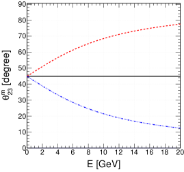
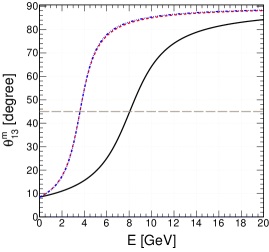
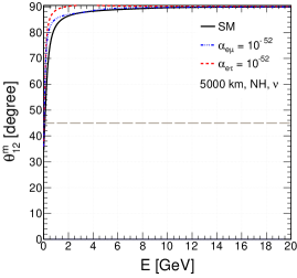
Figure 1: The variations in the effective mixing angles with the neutrino energy $E$ in the presence of $V_{CC}$ and $V_{e\mu/e\tau}$. The left, middle, and right panels depict the “running” of $\theta^{m}_{23}$, $\theta^{m}_{13}$, and $\theta^{m}_{12}$ respectively for $L$= 5000 km and NH. In each panel, the black solid line is for the SM case, whereas the blue dash-dotted and red dashed lines are for $\alpha_{e\mu}=10^{-52}$ and $\alpha_{e\tau}=10^{-52}$ respectively.

In Fig. 1, we plot the “running” of $\theta^{m}_{23}$ (left panel), $\theta^{m}_{13}$ (middle panel), and $\theta^{m}_{12}$ (right panel) as functions of the neutrino energy $E$. These plots are for neutrino with $L=5000$ km and NH. In each panel, we draw the curves for the following three cases: i) $\alpha_{e\mu}=\alpha_{e\tau}=0$ (the SM case), ii) $\alpha_{e\mu}=10^{-52}$, $\alpha_{e\tau}=0$ iii) $\alpha_{e\mu}=0$, $\alpha_{e\tau}=10^{-52}$. We repeat the same exercise for the effective mass-squared differences in Fig. 2. From the extreme right panel of Fig. 1, we can see that $\theta^{m}_{12}$ approaches to $90^{\circ}$ very rapidly as we increase $E$. This behavior is true for the SM case and as well as for non-zero $\alpha_{e\mu/e\tau}$, but it is not true for $\theta^{m}_{23}$ and $\theta^{m}_{13}$. The long-range potential $V_{e\mu/e\tau}$ affect the “running” of $\theta^{m}_{23}$ significantly as can be seen from the extreme left panel of Fig. 1. As we approach to higher energies, $\theta^{m}_{23}$ deviates from the maximal mixing and its value decreases (increases) very sharply for non-zero $\alpha_{e\mu}$ ($\alpha_{e\tau}$). This opposite behavior in “running” of $\theta^{m}_{23}$ for finite $\alpha_{e\mu}$ and $\alpha_{e\tau}$ affect the oscillation probabilities in different manner, which we discuss in next subsection. Note that $\theta^{m}_{23}$ is independent of $V_{CC}$ (see Eq. 16). Therefore, its value remains same for all the baselines and same is true for the SM case as well as for non-zero $\alpha_{e\mu/e\tau}$. In case of $\theta^{m}_{13}$ (see middle panel of Fig. 1), the impact of $V_{e\mu}$ and $V_{e\tau}$ are same and its “running“ is quite different as compared to $\theta^{m}_{23}$. Assuming NH, as we go to higher energies, $\theta^{m}_{13}$ quickly reaches to maximal mixing (resonance point) for both the symmetries as compared to the SM case. Finally, it approaches toward $90^{\circ}$ as we further increase the energy. For $\alpha_{e\mu/e\tau}=10^{-52}$, the resonance occurs around 3.5 GeV for 5000 km baseline. An analytical expression for the resonance energy can be obtained from Eq. 17 assuming $\theta^{m}_{13}=45^{\circ}$. In one mass scale dominance approximation ($\Delta m^{2}_{21}=0,\,i.e.\,\alpha=0$), the expression for the resonance energy $E_{\rm res}$ can be obtained from the following:

$$\lambda_{3}\,=\,A\,+\,W\,+\,\sin^{2}\theta_{13}\,.$$ (25)

Assuming $\alpha=0$ in Eqs. 19 and 16, we get a simplified expression of $\lambda_{3}$ which appears as

$$\lambda_{3}\,=\,\frac{1}{2}\,[\cos^{2}\theta_{13}-W+\sqrt{W^{2}_{e\tau}\,+\,\cos^{4}\theta_{13}}]\simeq\,\frac{1}{2}[2\cos^{2}\theta_{13}-W],$$ (26)

since at $E_{\rm res}$, the term $W^{2}$ is small compared to $\cos^{4}\theta_{13}$, and we can safely neglect it. Comparing Eq. 26 and Eq. 25, we obtain a simple and compact expression for $E_{\rm res}$:

$$E_{res}=\frac{\Delta m^{2}_{31}\,\cos 2\theta_{13}}{2V_{CC}\,+3V_{e\tau}}\,.$$ (27)

Note that in the absence of LRF, the above equation boils down to the well-known expression for $E_{\rm res}$ in the SM case. Also, we notice that the expression for resonance energy is same for both $L_{e}-L_{\tau}$ and $L_{e}-L_{\mu}$ symmetries (see Eq. 3.27 in Chatterjee:2015gta ). It is evident from Eq. 27 that for a fixed baseline, in the presence of $V_{e\mu/e\tau}$, the resonance takes place at lower energy as compared to the SM case (see middle panel of Fig. 1).

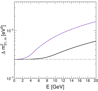
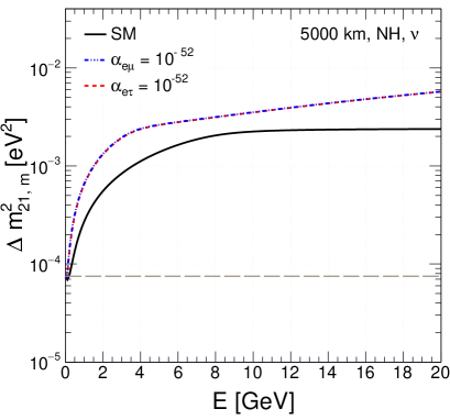
Figure 2: The variations in the $\Delta m^{2}_{31,m}$ ($\equiv m^{2}_{3,m}-m^{2}_{1,m}$, left panel) and $\Delta m^{2}_{21,m}$ ($\equiv m^{2}_{2,m}-m^{2}_{1,m}$, right panel) with the neutrino energy $E$ in presence of $V_{CC}$ and $V_{e\mu/e\tau}$ for $L$=5000 km and NH. We give plots for three different cases: i) $\alpha_{e\mu}=\alpha_{e\tau}=0$ (the SM case, black solid line), ii) $\alpha_{e\mu}=10^{-52}$, $\alpha_{e\tau}=0$ (blue dash-dotted line), and iii) $\alpha_{e\mu}=0$, $\alpha_{e\tau}=10^{-52}$ (red dashed line).

We observe from both the panels of Fig. 2 that in presence of LRF, the variations in $\Delta m^{2}_{31,m}$ and $\Delta m^{2}_{21,m}$ with energy are different as compared to the SM case. Interesting to note that both $V_{e\mu}$ and $V_{e\tau}$ modify the values of effective mass-squared differences in same fashion. In case of $\Delta m^{2}_{21,m}$ (see right panel of Fig. 2), it increases with energy and can be comparable to the vacuum value of $\Delta m^{2}_{31}$ at around $E=10$ GeV for both the SM and SM + LRF scenarios. For $\Delta m^{2}_{31,m}$ (see left panel of Fig. 2), the change with energy is very mild in the SM case, but in presence of LRF, $\Delta m^{2}_{31,m}$ gets increased substantially as we approach to higher energies. In case of antineutrino, the “running” of oscillation parameters can be obtained in the similar fashion by just replacing $A\rightarrow-A$ and $W\rightarrow-W$ in Eqs. 16 to 24. Next, we compare the neutrino and antineutrino oscillation probabilities obtained from our analytical expressions with those calculated numerically.

3.2 Comparison between Analytical and Numerical Results

We obtain the analytical probability expressions in the presence of $V_{CC}$ and $V_{e\mu/e\tau}$ by replacing the well known vacuum values of the elements of $U_{\rm PMNS}$ and the mass-squared differences $\Delta m^{2}_{ij}$ with their effective “running” values as discussed in the previous section.

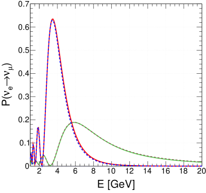
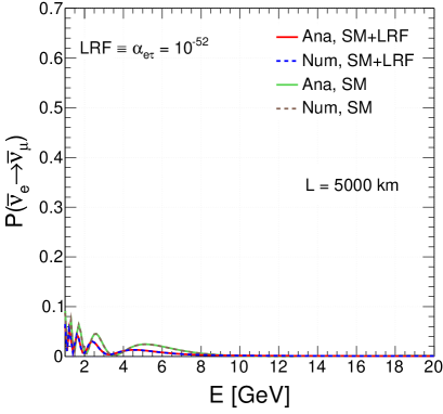
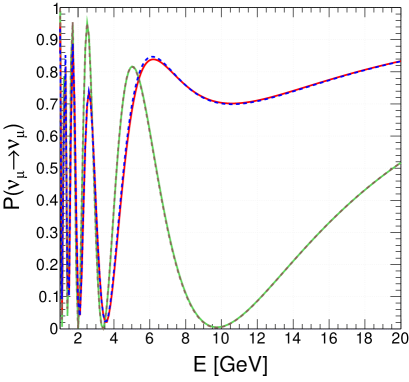
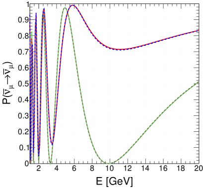
Figure 3: $\nu_{e}\rightarrow\nu_{\mu}$ ($\bar{\nu}_{e}\rightarrow\bar{\nu}_{\mu}$) transition probability for 5000 km in upper left (right) panel assuming NH. In bottom left (right) panel, we show $\nu_{\mu}\rightarrow\nu_{\mu}$ ($\bar{\nu}_{\mu}\rightarrow\bar{\nu}_{\mu}$) survival probability. In all the panels, we compare our analytical expressions (solid curves) to the exact numerical results (dashed curves) for the SM and SM + LRF cases. For LRF, we consider $\alpha_{e\tau}=10^{-52}$.

In Fig. 3, we show our approximate $\nu_{e}\rightarrow\nu_{\mu}$ ($\bar{\nu}_{e}\rightarrow\bar{\nu}_{\mu}$) oscillation probabilities in the top left (right) panel as a function of $E$ against the exact numerical results considering $L=5000$ km and NH. We repeat the same for $\nu_{\mu}\rightarrow\nu_{\mu}$ ($\bar{\nu}_{\mu}\rightarrow\bar{\nu}_{\mu}$) survival channels in bottom left (right) panel. We perform these comparisons among analytical (solid curves) and numerical (dashed curves) cases for both the SM and SM + LRF scenarios assuming our benchmark choice of $\alpha_{e\tau}=10^{-52}$. For $L_{e}-L_{\mu}$ symmetry, we perform the similar comparison in Fig. 9 (see appendix A). For the SM case ($\alpha_{e\tau}=0$), our approximate results match exactly with numerically obtained probabilities. In the presence of $L_{e}-L_{\tau}$ symmetry, we see that our analytical expressions work quite well and can produce almost accurate $L/E$ oscillation patterns.

We can see from the top left panel of Fig. 3 that for non-zero $\alpha_{e\tau}$, the location of the first oscillation maximum shifts toward lower energy (from 5.8 GeV to 3.5 GeV) and also its amplitude gets enhanced (from 0.18 to 0.64) for $\nu_{e}\rightarrow\nu_{\mu}$ transition probability assuming NH. To understand this feature, we can use the following simple expression for $P(\nu_{e}\rightarrow\nu_{\mu})$ considering $\theta^{m}_{12}=90^{\circ}$ (see right panel of Fig. 1):

$$P_{e\mu}=\sin^{2}\theta^{m}_{23}\,\sin^{2}2\theta^{m}_{13}\,\sin^{2}\frac{\Delta m^{2}_{32,m}\,L}{4E}\,.$$ (28)

As can be seen from the previous section, $\theta^{m}_{23}$ does not “run” for the SM case, but for non-zero $\alpha_{e\tau}$, it approaches toward $90^{\circ}$ as we increase $E$. As far as $\theta^{m}_{13}$ is concerned, it quickly reaches to the resonance point at a lower energy for non-zero $\alpha_{e\tau}$ as compared to $\alpha_{e\tau}=0$ case. Also, $\Delta m^{2}_{32,m}$ ($\Delta m^{2}_{31,m}-\Delta m^{2}_{21,m}$) decreases with energy as $\Delta m^{2}_{21,m}$ increases substantially in comparison to $\Delta m^{2}_{31,m}$ till $E\sim 4$ GeV for 5000 km baseline. All these different “running” of oscillation parameters are responsible to shift the location of first oscillation maximum toward lower energy and also to enhance its amplitude.

In case of $\nu_{\mu}\rightarrow\nu_{\mu}$ survival probability ($P_{\mu\mu}$), we can use the following simple expression assuming $\theta^{m}_{12}=90^{\circ}$:

$$P_{\mu\mu}=1-\sin^{2}2\theta^{m}_{23}\,\big{[}\cos^{2}\theta^{m}_{13}\sin^{2}\frac{\Delta m^{2}_{31,m}\,L}{4E}\,+\,\frac{1}{4}\tan^{2}\theta^{m}_{23}\sin^{2}2\theta^{m}_{13}\sin^{2}\frac{\Delta m^{2}_{32,m}\,L}{4E}$$

$$+\,\sin^{2}\theta^{m}_{13}\sin^{2}\frac{\Delta m^{2}_{21,m}\,L}{4E}\big{]}\,.$$ (29)

In the above expression, the term $\sin^{2}2\theta^{m}_{23}$ plays an important role. Now, we see from left panel of Fig. 1 that as we go to higher energies, $\theta^{m}_{23}$ deviates from the maximal mixing very sharply in presence of LRF. For this reason, the value of $\sin^{2}2\theta^{m}_{23}$ gets reduced substantially, which ultimately enhances the survival probability for non-zero $\alpha_{e\tau}$ as can be seen from the bottom left panel of Fig. 3. In the energy range of 6 to 20 GeV, we see a substantial enhancement in $P_{\mu\mu}$ with non-zero $\alpha_{e\tau}$ as compared to the SM case. The same is true for non-zero $\alpha_{e\mu}$ as can be seen from Fig. 9 in appendix A. We see a similar increase in case of $\bar{\nu}_{\mu}\rightarrow\bar{\nu}_{\mu}$ survival channel with NH (see bottom right panel of Fig. 3). We observe this behavior for other baselines as well in Figs. 5 and 6, which we discuss later.

4 Neutrino Oscillograms in ($E_{\nu}$, $\cos\theta_{\nu}$) Plane

The atmospheric neutrino experiments deal with a wide range of baselines and energies. Therefore, it is quite important to see how the long-range forces under discussion affect the neutrino oscillation probabilities for all possible choices of baseline ($\cos\theta_{\nu}$) and energy ($E_{\nu}$) which are relevant for the ICAL detector. We perform this study by drawing the neutrino oscillograms in ($E_{\nu},\,\cos\theta_{\nu}$) plane using the full three-flavor probability expressions with the varying Earth matter densities as given in the PREM profile PREM:1981 .

4.1 Oscillograms for $\nu_{e}\rightarrow\nu_{\mu}$ Appearance Channel

Fig. 4 shows the oscillograms for $\nu_{e}$ to $\nu_{\mu}$ appearance channel in $E_{\nu}$ and $\cos\theta_{\nu}$ plane assuming NH. We present the oscillograms for three different cases: i) extreme left panel is for the SM case ($\alpha_{e\mu}=\alpha_{e\tau}=0$), ii) middle panel is for the SM + LRF ($\alpha_{e\mu}=10^{-52}$), and iii) extreme right panel deals with the SM + LRF ($\alpha_{e\tau}=10^{-52}$). For the SM case, $\nu_{e}$ to $\nu_{\mu}$ transition probability attains the maximum value around the resonance region which occurs in the range of $E\in$ 4 to 8 GeV and $\cos\theta_{\nu}\in$ -0.8 to -0.4. The resonance condition in presence of LRF (see Eq. 27) suggests that $\theta^{m}_{13}$ can reach $45^{\circ}$ at smaller energies and baselines as compared to the SM case. This feature gets reflected in the middle and right panels of Fig. 4 for non-zero $\alpha_{e\mu}$ and $\alpha_{e\tau}$ respectively.

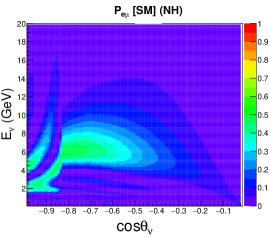
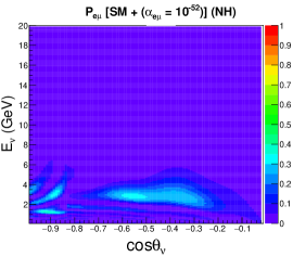
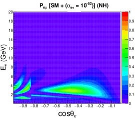
Figure 4: The oscillograms for $\nu_{e}\rightarrow\nu_{\mu}$ channel in $E_{\nu}$, $\cos\theta_{\nu}$ plane for three different scenario: i) $\alpha_{e\mu}=\alpha_{e\tau}=0$ (the SM case, left panel), ii) $\alpha_{e\mu}=10^{-52}$, $\alpha_{e\tau}=0$ (middle panel), and iii) $\alpha_{e\mu}=0$, $\alpha_{e\tau}=10^{-52}$ (right panel). Here, in all the panels, we assume NH.

Fig. 4 also depicts that the value of $P_{e\mu}$ decreases (increases) as compared to the SM case for non-zero $\alpha_{e\mu}$ ($\alpha_{e\tau}$). We can explain this behavior from the “running” of $\theta^{m}_{23}$ (see left panel of Fig. 1). In presence of $L_{e}-L_{\mu}$ ($L_{e}-L_{\tau}$) symmetry, the term $\sin^{2}\theta^{m}_{23}$ in Eq. 28 gets reduced (enhanced) as compared to the SM case, which subsequently decreases (increases) the value of $P_{e\mu}$.

4.2 Oscillograms for $\nu_{\mu}\rightarrow\nu_{\mu}$ Disappearance Channel

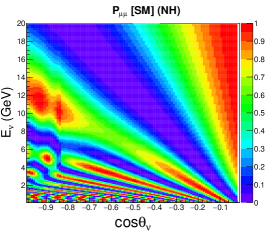
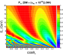
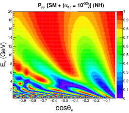
Figure 5: The oscillograms for $\nu_{\mu}\rightarrow\nu_{\mu}$ channel in $E_{\nu}$, $\cos\theta_{\nu}$ plane for three different scenario: i) $\alpha_{e\mu}=\alpha_{e\tau}=0$ (the SM case, left panel), ii) $\alpha_{e\mu}=10^{-52}$, $\alpha_{e\tau}=0$ (middle panel), and iii) $\alpha_{e\mu}=0$, $\alpha_{e\tau}=10^{-52}$ (right panel). Here, in all the panels, we assume NH.

In Fig. 5, we present the oscillograms for $\nu_{\mu}$ survival channel in the plane of $\cos\theta_{\nu}$ vs. $E_{\nu}$ considering NH. Here, we draw the oscillograms for the same three cases as considered in Fig. 4. First, we notice that for $E_{\nu}$ in the range of 6 to 20 GeV and $\cos\theta_{\nu}$ in the range of -1 to -0.2, survival probability $P_{\mu\mu}$ gets enhanced significantly for both non-zero $\alpha_{e\mu}$ (middle panel) and $\alpha_{e\tau}$ (right panel) as compared to the SM case (see left panel). The reason is the following. As we move to higher energies, $\theta^{m}_{23}$ deviates from maximal mixing for both non-zero $\alpha_{e\mu}$ and $\alpha_{e\tau}$. As a result, the term $\sin^{2}2\theta^{m}_{23}$ in Eq. 29 gets reduced and causes an enhancement in $P_{\mu\mu}$. In Fig. 5, we see some differences in the oscillogram patterns in the energy range of 2 to 5 GeV for $L_{e}-L_{\mu}$ (middle panel) and $L_{e}-L_{\tau}$ (right panel) symmetries. Let us try to understand the reason behind this. We have already seen that $\theta^{m}_{23}$ “runs” in the opposite directions from $45^{\circ}$ for $L_{e}-L_{\mu}$ and $L_{e}-L_{\tau}$ symmetries. Due to this, the only term $\frac{1}{4}\tan^{2}\theta^{m}_{23}\,\sin^{2}2\theta^{m}_{13}$ in Eq. 29 gives different contributions for finite $\alpha_{e\mu}$ and $\alpha_{e\tau}$. Around the resonance region ($E\sim$ 2 to 5 GeV), $\theta^{m}_{13}$ attains the maximal value, and the strength of above mentioned term becomes quite significant which causes the differences in $P_{\mu\mu}$ for these two U(1) symmetries under consideration. We see the effect of this feature in the top left panel of Fig. 6, which we discuss later.

5 Important Features of the ICAL detector

The proposed Iron Calorimeter (ICAL) detector Kumar:2017sdq under the India-based Neutrino Observatory (INO) INO project plans to study the fundamental properties of atmospheric neutrino and antineutrino separately using the magnetic field inside the detector. The strength of the magnetic field will be around 1.5 T with a better uniformity in the central region Behera:2014zca . It helps to determine the charges of $\mu^{-}$ and $\mu^{+}$ particles which get produced in the charged-current (CC) interactions of $\nu_{\mu}$ and $\bar{\nu}_{\mu}$ inside the ICAL detector. To restrict the cosmic muons, which serve as background in our case, the ICAL detector is planned to have rock coverage of more than 1 km all around. According to the latest design of the ICAL detector Kumar:2017sdq ; INO , it consists of alternate layers of iron plates and glass Resistive Plate Chambers (RPCs) Datar:2009zz , which act as the target material and active detector elements respectively. While passing through the RPCs, the minimum ionizing particle muon gives rise to a distinct track, whose path is recorded in terms of strip hits. We identify these tracks with the help of a track finding algorithm. Then, we reconstruct the momentum and charge of muon using the well known Kalman Filter Bhattacharya:2014tha ; Bhattacharya:2015odk package. The typical detection efficiency of a 5 GeV muon in ICAL traveling vertically is around $80\%$, while the achievable charge identification efficiency is more than $95\%$ Chatterjee:2014vta . In ICAL, the energy resolution ($\sigma/E$) of a 5 to 10 GeV muon varies in the range of $10\%$ to $15\%$, while its direction may be reconstructed with an accuracy of one degree Chatterjee:2014vta . The prospects of ICAL to measure the three-flavor oscillation parameters based on the observable ($E_{\mu},\cos\theta_{\mu}$) have already been studied in Ref. Ghosh:2012px ; Thakore:2013xqa .

The hits in the RPCs due to hadrons produce shower-like features. Recently, the possibilities of detecting hadron shower and measuring its energy in ICAL have been explored Devi:2013wxa ; Mohan:2014qua . These final state hadrons get produced along with the muons in CC deep-inelastic scattering process in multi-GeV energies, and can provide vital information about the initial neutrino. We can calibrate the energy of hadron ($E^{{}^{\prime}}_{had}=E_{\nu}-E_{\mu}$) using number of hits produced by hadron showers Devi:2013wxa . Preliminary studies have shown that one can achieve an energy resolution of 85$\%$ ($36\%$) at 1 GeV (15 GeV). Combining the muon ($E_{\mu},\cos\theta_{\mu}$) and hadron ($E^{{}^{\prime}}_{had}$) information on an event-by-event basis, the physics reach of ICAL to the neutrino oscillation parameters can be improved significantly Devi:2014yaa . We follow the Refs. Chatterjee:2014vta and Devi:2013wxa to incorporate the detector response for muons and hadrons respectively.

6 Event Spectrum in the ICAL Detector

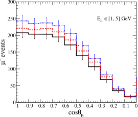
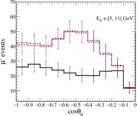
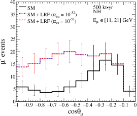
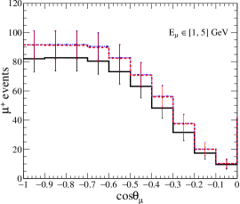
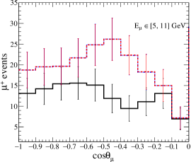
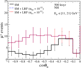
Figure 6: The distributions of $\mu^{-}$ (upper panels) and $\mu^{+}$ (lower panels) events for three different $E_{\mu}$ bins: 1 to 5 GeV in left panel, 5 to 11 GeV in middle panel, and 11 to 21 GeV in right panel. In each panel, we consider three different cases: i) $\alpha_{e\mu}=\alpha_{e\tau}=0$ (the SM case, black solid line), ii) $\alpha_{e\mu}=10^{-52}$, $\alpha_{e\tau}=0$ (blue dash-dotted line), and iii) $\alpha_{e\mu}=0$, $\alpha_{e\tau}=10^{-52}$ (red dashed line). Here, we sum over $E^{{}^{\prime}}_{had}$ in its entire range of 0 to 25 GeV and show the results for 500 kt$\cdot$yr exposure and assuming NH.

In this section, we present the expected event spectra and total event rates in ICAL with and without long-range forces. Using the event generator NUANCE Casper:2002sd and atmospheric neutrino fluxes at Kamioka Honda:2011nf , we obtain the unoscillated event spectra for neutrino and antineutrino. After incorporating the detector response for muons and hadrons as described in Ref. Devi:2014yaa and for the benchmark values of the oscillation parameters as mentioned in section 3.1 ($\sin^{2}\theta_{23}=0.5$, $\,\sin^{2}2\theta_{13}=0.0847$, and NH), we obtain around 4870 (2187) $\mu^{-}$ ($\mu^{+}$) events for the SM case using a 500 kt$\cdot$yr exposure. To obtain these event rates, we consider $E_{\mu}$ in the range 1 to 21 GeV, $\cos\theta_{\mu}$ in its entire range of -1 to 1, and $E^{{}^{\prime}}_{had}$ in the range 0 to 25 GeV. In presence of $L_{e}-L_{\mu}$ symmetry with $\alpha_{e\mu}=10^{-52}$, the number of $\mu^{-}$ ($\mu^{+}$) events becomes 5365 (2373). For $L_{e}-L_{\tau}$ symmetry with $\alpha_{e\tau}=10^{-52}$, we get 5225 $\mu^{-}$ and 2369 $\mu^{+}$ events. In Fig. 6, we show the distribution of only upward going $\mu^{-}$ (top panels) and $\mu^{+}$ (bottom panels) events as a function of reconstructed $\cos\theta_{\mu}$ in the range -1 to 0. Here, we integrate over the entire range of hadron energy ($E^{{}^{\prime}}_{had}\in$ 0 to 25 GeV), and display the event spectra considering three different $E_{\mu}$ bins having the ranges 1 to 5 GeV (left panels), 5 to 11 GeV (middle panels), and 11 to 21 GeV (right panels). In each panel, we compare the event distribution for three different scenarios: i) $\alpha_{e\mu}=\alpha_{e\tau}=0$ (the SM case, black solid lines), ii) $\alpha_{e\mu}=10^{-52}$, $\alpha_{e\tau}=0$ (blue dash-dotted lines), and iii) $\alpha_{e\mu}=0$, $\alpha_{e\tau}=10^{-52}$ (red dashed lines). We observe few interesting features in Fig. 6, which we discuss now.

In all the panels of Fig. 6, we see an enhancement in the event rates for $\cos\theta_{\mu}\in$ -1 to -0.2 in the presence of long-range forces as compared to the SM case. This mainly happens due to substantial increase in $P_{\mu\mu}$ with finite $\alpha_{e\mu}$ or $\alpha_{e\tau}$ as compared to the SM case. We have already seen this feature in Fig. 5. Also, we see similar event distributions for both the symmetries in all the panels, except in the top left panel ($E_{\mu}\in$ 1 to 5 GeV), where we see some differences in the event spectra for $L_{e}-L_{\mu}$ and $L_{e}-L_{\tau}$ symmetries. We have already explained the reason behind this with the help of oscillogram patterns (see middle and right panels in Fig. 5) in section 4.2. Next, we discuss the binning scheme for three observables ($E_{\mu}$, $\cos\theta_{\mu}$, and $E^{\prime}_{had}$), and briefly describe the numerical technique and analysis procedure which we adopt to estimate the physics reach of ICAL.

7 Simulation Procedure

7.1 Binning Scheme for Observables ($E_{\mu}$, $\cos\theta_{\mu}$, $E^{\prime}_{had}$)

Observable	Range	Bin width	No. of bins	Total bins
$E_{\mu}$ (GeV)	$[1,11]$ $[11,21]$	1 5	10 2	12
$\cos\theta_{\mu}$	$[-1.0,0.0]$ $[0.0,1.0]$	0.1 0.2	10 5	15
$E^{\prime}_{\rm had}$ (GeV)	$[0,2]$ $[2,4]$ $[4,25]$	1 2 21	2 1 1	4

Table 2: The binning scheme considered for the reconstructed observables $E_{\mu}$, $\cos\theta_{\mu}$, and $E^{\prime}_{had}$ for each muon polarity. In last column, we give the total number of bins taken for each observable.

Table 2 shows the binning scheme that we adopt in our simulation for three observables $E_{\mu}$ ($\in$ 1 to 21 GeV), $\cos\theta_{\mu}$ ($\in$ -1 to 1), and $E^{\prime}_{had}$ ($\in$ 0 to 25 GeV). In these ranges, we have total 12 bins for $E_{\mu}$, 15 bins for $\cos\theta_{\mu}$, and 4 bins for $E^{\prime}_{had}$, resulting into a total of ($12\times 15\times 4=$) 720 bins per polarity. We consider the same binning scheme for $\mu^{-}$ and $\mu^{+}$ events. As we go to higher energies, the atmospheric neutrino flux decreases resulting in lower statistics. Therefore, we take wider bins for $E_{\mu}$ and $E^{\prime}_{had}$ at higher energies. We do not perform any optimization study for binning, however we make sure that we have sufficient statistics in most of the bins without diluting the sensitivity much. In our study, the upward going events ($\cos\theta_{\mu}$ in the range 0 to -1) play an important role, where $V_{CC}$, $V_{e\mu/e\tau}$, and $\Delta m^{2}_{31}/2E$ become comparable and can interfere with each other (see discussion in section 3). Therefore, we take 10 bins of equal width for upward going events which is compatible with the angular resolutions of muon achievable in ICAL. The downward going events do not undergo oscillations. But, they certainly enhance the overall statistics and help us to reduce the impact of normalization uncertainties in the atmospheric neutrino fluxes. Therefore, we include the downward going events in our simulation considering five $\cos\theta_{\mu}$ bins of equal width in the range of 0 to 1.

7.2 Numerical Analysis

In our numerical analysis, we suppress the statistical fluctuations of the “observed” event distribution. We generate events using NUANCE for an exposure of 50000 kt$\cdot$yr. Then, we implement the detector response and finally, normalize the event distribution to the actual exposure. This method along with the $\chi^{2}$ function gives us the median sensitivity of the experiment in the frequentist approach Blennow:2013oma . We use the following Poissonian $\chi^{2}_{-}$ for $\mu^{-}$ events in our statistical analysis:

$$\chi^{2}_{-}\,=\,\min_{\zeta_{l}}\,\sum^{N_{E^{\prime}_{had}}}_{i=1}\sum^{N_{E_{\mu}}}_{j=1}\sum^{N_{{\cos\theta_{\mu}}}}_{k=1}\,2\,\bigg{[}N^{\rm theory}_{ijk}\,-\,N^{\rm data}_{ijk}\,-\,N^{\rm data}_{ijk}\,\,{\rm{ln}}\bigg{(}\frac{N^{\rm theory}_{ijk}}{N^{\rm data}_{ijk}}\bigg{)}\bigg{]}\,+\,\sum^{5}_{l=1}\zeta^{2}_{l}\,,$$ (30)

with

$$N^{\rm theory}_{ijk}\,=\,N^{0}_{ijk}\big{(}\,1\,+\,\sum^{5}_{l=1}\pi^{l}_{ijk}\zeta_{l}\,\big{)}\,.$$ (31)

In the above equation, $N^{\rm data}_{ijk}$ and $N^{\rm theory}_{ijk}$ denote the “observed” and expected number of $\mu^{-}$ events in a given ($E_{\mu}$, $\cos\theta_{\mu}$, $E^{\prime}_{had}$) bin. $N^{0}_{ijk}$ represents the number of events without systematic uncertainties. In our simulation, $N_{E^{\prime}_{had}}=4$, $N_{E_{\mu}}=12$, and $N_{{\cos\theta_{\mu}}}=15$ (see table 2). We obtain $N^{\rm data}_{ijk}$ using the benchmark values of the oscillation parameters as mentioned in section 3.1 and assuming normal hierarchy as neutrino mass hierarchy. We consider five systematic errors in our analysis: 20$\%$ flux normalization error, 10$\%$ error in cross-section, 5$\%$ tilt error, 5$\%$ zenith angle error, and 5$\%$ overall systematics. We incorporate these systematic uncertainties in our simulation using the well known “pull” method Huber:2002mx ; Fogli:2002pt ; GonzalezGarcia:2004wg .

In a similar fashion, we obtain $\chi^{2}_{+}$ for $\mu^{+}$ events. We estimate the total $\chi^{2}$ by adding the individual contributions coming from $\mu^{-}$ and $\mu^{+}$ events in the following way

$$\chi^{2}_{\rm ICAL}=\chi^{2}_{-}\,+\,\chi^{2}_{+}\,.$$ (32)

In the fit, we first minimize $\chi^{2}_{\rm ICAL}$ with respect to the pull variables $\zeta_{l}$, and then marginalize over the oscillation parameters $\sin^{2}\theta_{23}$ in the range $0.38$ to $0.63$ and $\Delta m^{2}_{31}$ in the range 0.0024 eV² to 0.0026 eV². While deriving the constraints on $\alpha_{e\mu/e\tau}$, we also marginalize $\chi^{2}_{\rm ICAL}$ over both NH and IH. We do not marginalize over $\Delta m^{2}_{21}$, $\sin^{2}\theta_{12}$, and $\sin^{2}2\theta_{13}$ since these parameters are already measured with high precision, and the existing uncertainties on these parameters do not alter our results. We consider $\delta_{\rm CP}=0^{\circ}$ throughout our analysis.

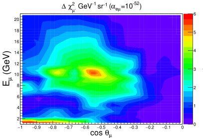
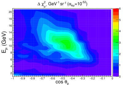
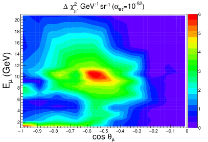
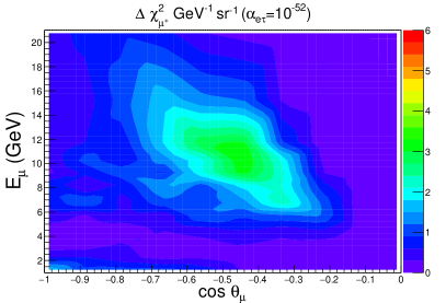
Figure 7: Distributions of $\Delta\chi^{2}_{\rm ICAL-LRF}$ (per unit area) in $E_{\mu}$ and $\cos\theta_{\mu}$ plane. The left (right) panels are for $\mu^{-}$ ($\mu^{+}$) events. In upper (lower) panels, we assume non-zero $\alpha_{e\mu}$ ($\alpha_{e\tau}$) in the fit with a strength of $10^{-52}$. In all the panels, we use 500 kt$\cdot$yr exposure and assume NH in both data and theory.

8 Results

We quantify the statistical significance of the analysis to constrain the LRF parameters in the following way

$$\Delta\chi^{2}_{\,\,{\rm ICAL-LRF}}=\chi^{2}_{\,\,{\rm ICAL}}\left({\rm SM}+\alpha_{e\mu/e\tau}\right)-\chi^{2}_{\,\,{\rm ICAL}}\left({\rm SM}\right)\,.$$ (33)

Here, $\chi^{2}_{\,\,{\rm ICAL}}({\rm SM})$ and $\chi^{2}_{\,\,{\rm ICAL}}\left({\rm SM}+\alpha_{e\mu/e\tau}\right)$ are calculated by fitting the “observed” data in the absence and presence of LRF parameters respectively. In our analysis, statistical fluctuations are suppressed, and therefore, $\chi^{2}_{\,\,{\rm ICAL}}({\rm SM})\approx 0$. Before we present the constraints on $\alpha_{e\mu/e\tau}$, we identify the regions in $E_{\mu}$ and $\cos\theta_{\mu}$ plane which give significant contributions toward $\Delta\chi^{2}_{\,\,{\rm ICAL-LRF}}$. In Fig. 7, we show the distribution of $\Delta\chi^{2}_{\mu^{-}}$ (left panels) and $\Delta\chi^{2}_{\mu^{+}}$ (right panels) in the reconstructed $E_{\mu}$ and $\cos\theta_{\mu}$ plane, where the events are further divided into four sub-bins depending on the reconstructed hadron energy (see table 2). In the upper (lower) panels of Fig. 7, we take non-zero $\alpha_{e\mu}$ ($\alpha_{e\tau}$) in the fit with a strength of $10^{-52}$. We clearly see from the left panels that for $\mu^{-}$ events, most of the contributions ($\sim 70\%$) stem from the range 6 to 15 GeV for $E_{\mu}$ and for $\cos\theta_{\mu}$, the effective range is -0.8 to -0.4. We see similar trend for both the symmetries (see upper and lower panels) and for $\mu^{+}$ events (see right panels) as well.

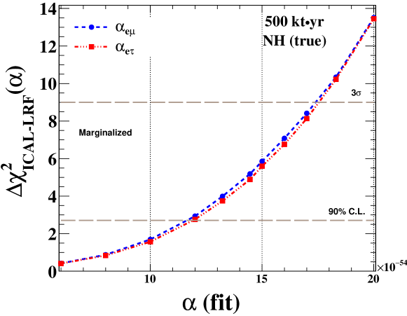
Figure 8: Sensitivity of ICAL to set upper limits on $\alpha_{e\mu}$ (blue dashed line) and $\alpha_{e\tau}$ (red dash-dotted line) using 500 kt$\cdot$yr exposure and assuming NH as true choice.

Fig. 8 shows the upper bound on $\alpha_{e\mu}$ and $\alpha_{e\tau}$ (one at-a-time) using 500 kt$\cdot$yr exposure of ICAL if there is no signal of long-range forces in the data. We set new upper limit on $\alpha_{e\mu}$ or $\alpha_{e\tau}$ by generating the data with no long-range forces and fitting it with some non-zero value of $\alpha_{e\mu/e\tau}$ by means of $\chi^{2}$ technique as outlined in previous section. The corresponding $\Delta\chi^{2}_{\,\,{\rm ICAL-LRF}}$ obtained after marginalizing over $\sin^{2}\theta_{23}$, $\Delta m^{2}_{31}$, hierarchy, and systematics parameters in the fit, is plotted in Fig. 8 as a function of $\alpha_{e\mu/e\tau}$ (test). It gives a measure of the sensitivity reach of ICAL to the effective gauge coupling of LRF. For both the symmetries, we assume NH as true hierarchy. We obtain similar constraints for both the symmetries (one at-a-time) since $\alpha_{e\mu}$ and $\alpha_{e\tau}$ affect both $P_{\mu\mu}$ and $P_{e\mu}$ oscillation channels in almost similar fashion over a wide range of energies and baselines (see Figs. 4 and 5). The expected upper limit on $\alpha_{e\mu/e\tau}$ from ICAL is $<1.2\times 10^{-53}$ ($1.75\times 10^{-53}$) at 90$\%$ (3$\sigma$) C.L. with 500 kt$\cdot$yr exposure and NH as true hierarchy. This future limit on $\alpha_{e\mu}$ from ICAL at 90$\%$ C.L. is $\sim$ 46 times better than the existing limit from the Super-Kamiokande experiment Joshipura:2003jh . For $\alpha_{e\tau}$, the limit is 53 times better at 90$\%$ confidence level. We obtain similar constraints assuming IH as true hierarchy. We see a marginal improvement in the upper limits if we keep all the oscillation parameters fixed in the fit. In this fixed parameter case, the new bound becomes $\alpha_{e\mu}<1.63\times 10^{-53}$ at $3\sigma$ confidence level. We study few interesting issues in this fixed parameter scenario which we discuss now.

• Advantage of Spectral Information: In ICAL, we can bin the atmospheric neutrino/antineutrino events in the observables $E_{\mu}$, $\cos\theta_{\mu}$, and $E^{\prime}_{had}$. It helps us immensely to achieve hierarchy measurement at around $3\sigma$ C.L. with 500 kt$\cdot$yr exposure Devi:2014yaa . We find that the ability of using the spectral information in ICAL also plays an important role to place tight constraint on LRF parameters. For an example, if we rely only on the total $\mu^{-}$ and $\mu^{+}$ event rates, the expected limit from ICAL becomes $\alpha_{e\mu}<2.2\times 10^{-52}$ at 3$\sigma$ confidence level. This limit is almost 13 times weaker as compared to what we can obtain using the full spectral informations.

• Usefulness of Hadron Energy Information: In our analysis, we use the hadron energy information ($E^{\prime}_{had}$) along with the muon momentum ($E_{\mu}$, $\cos\theta_{\mu}$). We observe that with a value of $\alpha_{e\mu}=1.63\times 10^{-53}$ in the fit, $\Delta\chi^{2}_{\rm ICAL-LRF}$ increases from 5.2 to 9 when we use $E_{\mu}$, $\cos\theta_{\mu}$, and $E^{\prime}_{had}$ as our observables instead of only $E_{\mu}$ and $\cos\theta_{\mu}$. It corresponds to about 73$\%$ improvement in the sensitivity.

• The Role of Charge Identification Capability: We also find that the charge identification capability of ICAL in distinguishing $\mu^{-}$ and $\mu^{+}$ events does not play an important role to constrain the LRF parameters unlike the mass hierarchy measurements. Since the long-range forces affect the $\mu^{-}$ and $\mu^{+}$ event rates in almost similar fashion as compared to the SM case (see Fig 6), it is not crucial to separate these events in our analysis in constraining the LRF parameters.

Before we summarize and draw our conclusions in the next section, we make few comments on how the presence of LRF parameters may affect the mass hierarchy measurement in ICAL. To perform this study, we generate the data with a given hierarchy and assuming $\alpha_{e\mu}=\alpha_{e\tau}=0$. Then, while fitting the “observed” event spectrum with the opposite hierarchy, we introduce $\alpha_{e\mu}$ or $\alpha_{e\tau}$ (one at-a-time) in the fit and marginalize over it in the range of $10^{-55}$ to $10^{-52}$ along with other oscillation parameters. During this analysis, we find that the mass hierarchy sensitivity of ICAL gets reduced very marginally by around 5%.

9 Summary and Conclusions

The main goal of the proposed ICAL experiment at INO is to measure the neutrino mass hierarchy by observing the atmospheric neutrinos and antineutrinos separately and making use of the Earth matter effects on their oscillations. Apart from this, ICAL detector can play an important role to unravel various new physics scenarios beyond the SM (see Refs. Dash:2014sza ; Dash:2014fba ; Chatterjee:2014oda ; Chatterjee:2014gxa ; Choubey:2015xha ; Behera:2016kwr ; Choubey:2017eyg ; Choubey:2017vpr ). In this paper, we have studied in detail the capabilities of ICAL to constrain the flavor-dependent long-range leptonic forces mediated by the extremely light and neutral bosons associated with gauged $L_{e}-L_{\mu}$ or $L_{e}-L_{\tau}$ symmetries. It constitutes a minimal extension of the SM preserving its renormalizibility and may alter the expected event spectrum in ICAL. As an example, the electrons inside the sun can generate a flavor-dependent long-range potential $V_{e\mu/e\tau}$ at the Earth surface, which may affect the running of oscillation parameters in presence of the Earth matter. Important point to note here is that for atmospheric neutrinos, $\Delta m^{2}/2E\sim$ 2.5$\times$ $10^{-13}$ (assuming $\Delta m^{2}\sim 2.5\times 10^{-3}$ eV² and $E$ = 5 GeV), which is comparable to $V_{e\mu/e\tau}$ even for $\alpha_{e\mu/e\tau}\sim 10^{-52}$, and can influence the atmospheric neutrino experiments significantly. Also, for a wide range of baselines accessible in atmospheric neutrino experiments, the Earth matter potentials ($V_{CC}$) are around $10^{-13}$ eV (see table 1), suggesting that $V_{CC}$ can interfere with $V_{e\mu/e\tau}$ and $\Delta m^{2}_{31}/2E$, and can modify the oscillation probability substantially. In this article, we have explored these interesting possibilities in the context of the ICAL detector.

After deriving approximate analytical expressions for the effective neutrino oscillation parameters in presence of $V_{CC}$ and $V_{e\mu/e\tau}$, we compare the oscillation probabilities obtained using our analytical expressions with those calculated numerically. Then, we have studied the impact of long-range forces by drawing the neutrino oscillograms in $E_{\nu}$ and $\cos\theta_{\nu}$ plane using the full three-flavor probability expressions with the varying Earth matter densities based on the PREM profile PREM:1981 . We have also presented the expected event spectra and total event rates in ICAL with and without long-range forces. As non-zero $\alpha_{e\mu}$ and $\alpha_{e\tau}$ can change the standard 3$\nu$ oscillation picture of ICAL significantly, we can expect to place strong limits on these parameters if ICAL do not observe a signal of LRF in oscillations. The expected upper bound on $\alpha_{e\mu/e\tau}$ from ICAL is $<1.2\times 10^{-53}$ ($1.75\times 10^{-53}$ ) at 90$\%$ (3$\sigma$) C.L. with 500 kt$\cdot$yr exposure and NH as true hierarchy. ICAL’s limit at 90$\%$ C.L. on $\alpha_{e\mu}$ ($\alpha_{e\tau}$) is $\sim 46$ (53) times better than the existing limit from the Super-Kamiokande experiment. Here, we would like to mention that if the range of LRF is equal or larger than our distance from the Galactic Center, then the collective long-range potential due to all the electrons inside the Galaxy needs to be taken into accountPhysRevD.75.093005 . In such cases, ICAL can be sensitive to even lower values of $\alpha_{e\mu/e\tau}$. We hope that our present work can be an important addition to the series of interesting physics studies which can be performed using the proposed ICAL detector at the India-based Neutrino Observatory.

10 Acknowledgment

This work is a part of the ongoing effort of INO-ICAL Collaboration to study various physics potentials of the proposed ICAL detector. Many members of the Collaboration have contributed for the completion of this work. We would like to thank A. Dighe, A.M. Srivastava, P. Agrawal, S. Goswami, P.K. Behera, D. Indumathi for their useful comments on our work. We acknowledge S.S. Chatterjee for many useful discussions during this work. We thank A. Kumar and B.S. Acharya for helping us during the INO Internal Review Process. A.K. would like to thank the Department of Atomic Energy (DAE), Government of India for financial support. S.K.A. acknowledges the support from DST/INSPIRE Research Grant No. IFA-PH-12.

Appendix A Oscillation Probability with $L_{e}-L_{\mu}$ Symmetry

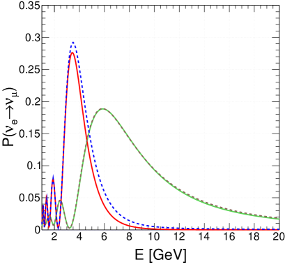
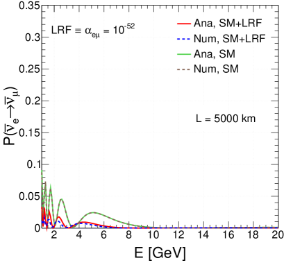
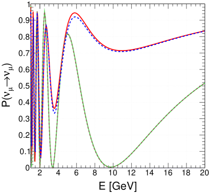
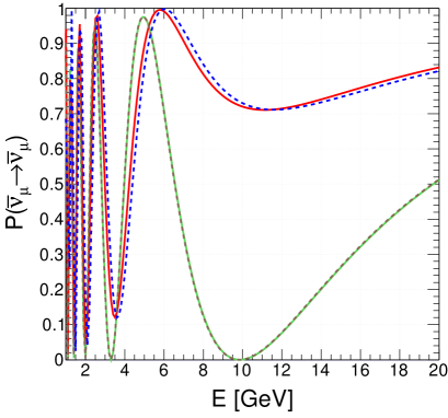
Figure 9: $\nu_{e}\rightarrow\nu_{\mu}$ ($\bar{\nu}_{e}\rightarrow\bar{\nu}_{\mu}$) transition probability for 5000 km in upper left (right) panel assuming NH. In bottom left (right) panel, we show $\nu_{\mu}\rightarrow\nu_{\mu}$ ($\bar{\nu}_{\mu}\rightarrow\bar{\nu}_{\mu}$) survival probability. In all the panels, we compare our analytical expressions (solid curves) to the exact numerical results (dashed curves) for the SM and SM + LRF cases. For LRF, we consider $\alpha_{e\mu}=10^{-52}$.

Fig. 9 shows approximate $\nu_{e}\rightarrow\nu_{\mu}$ ($\bar{\nu}_{e}\rightarrow\bar{\nu}_{\mu}$) oscillation probabilities in the top left (right) panel as a function of $E$ against the exact numerical results considering $L=5000$ km and NH. We repeat the same for $\nu_{\mu}\rightarrow\nu_{\mu}$ ($\bar{\nu}_{\mu}\rightarrow\bar{\nu}_{\mu}$) survival channels in bottom left (right) panel. We perform these comparisons among analytical (solid curves) and numerical (dashed curves) cases for both the SM and SM + LRF scenarios considering our benchmark choice of $\alpha_{e\mu}=10^{-52}$. For the SM case ($\alpha_{e\mu}=0$), the approximate results match exactly with numerically obtained probabilities. Analytical expressions also work quite well in presence of $L_{e}-L_{\mu}$ symmetry, and can produce almost accurate $L/E$ oscillation patterns.

References

- (1) Particle Data Group Collaboration, C. Patrignani et al., Review of Particle Physics, Chin. Phys. C40 (2016), no. 10 100001.
- (2) I. Esteban, M. C. Gonzalez-Garcia, M. Maltoni, I. Martinez-Soler, and T. Schwetz, Updated fit to three neutrino mixing: exploring the accelerator-reactor complementarity, JHEP 01 (2017) 087, [arXiv:1611.01514].
- (3) P. F. de Salas, D. V. Forero, C. A. Ternes, M. Tortola, and J. W. F. Valle, Status of neutrino oscillations 2017, arXiv:1708.01186.
- (4) F. Capozzi, E. Di Valentino, E. Lisi, A. Marrone, A. Melchiorri, and A. Palazzo, Global constraints on absolute neutrino masses and their ordering, arXiv:1703.04471.
- (5) NuFIT webpage, http://www.nu-fit.org/.
- (6) S. Pascoli and T. Schwetz, Prospects for neutrino oscillation physics, Adv.High Energy Phys. 2013 (2013) 503401.
- (7) S. K. Agarwalla, S. Prakash, and S. Uma Sankar, Exploring the three flavor effects with future superbeams using liquid argon detectors, JHEP 1403 (2014) 087, [arXiv:1304.3251].
- (8) S. K. Agarwalla, Physics Potential of Long-Baseline Experiments, Adv.High Energy Phys. 2014 (2014) 457803, [arXiv:1401.4705].
- (9) NOvA Collaboration, P. Adamson et al., Measurement of the neutrino mixing angle in NOvA, Phys. Rev. Lett. 118 (2017), no. 15 151802, [arXiv:1701.05891].
- (10) Super-Kamiokande Collaboration, K. Abe et al., Atmospheric neutrino oscillation analysis with external constraints in Super-Kamiokande I-IV, arXiv:1710.09126.
- (11) ICAL Collaboration, S. Ahmed et al., Physics Potential of the ICAL detector at the India-based Neutrino Observatory (INO), Pramana 88 (2017), no. 5 79, [arXiv:1505.07380].
- (12) India-based Neutrino Observatory (INO), http://www.ino.tifr.res.in/ino/.
- (13) L. Wolfenstein, Neutrino Oscillations in Matter, Phys.Rev. D17 (1978) 2369–2374.
- (14) S. Mikheev and A. Y. Smirnov, Resonance Amplification of Oscillations in Matter and Spectroscopy of Solar Neutrinos, Sov.J.Nucl.Phys. 42 (1985) 913–917.
- (15) S. Mikheev and A. Y. Smirnov, Resonant amplification of neutrino oscillations in matter and solar neutrino spectroscopy, Nuovo Cim. C9 (1986) 17–26.
- (16) A. Ghosh, T. Thakore, and S. Choubey, Determining the Neutrino Mass Hierarchy with INO, T2K, NOvA and Reactor Experiments, JHEP 1304 (2013) 009, [arXiv:1212.1305].
- (17) T. Thakore, A. Ghosh, S. Choubey, and A. Dighe, The Reach of INO for Atmospheric Neutrino Oscillation Parameters, JHEP 05 (2013) 058, [arXiv:1303.2534].
- (18) M. M. Devi, T. Thakore, S. K. Agarwalla, and A. Dighe, Enhancing sensitivity to neutrino parameters at INO combining muon and hadron information, JHEP 1410 (2014) 189, [arXiv:1406.3689].
- (19) A. Ajmi, A. Dev, M. Nizam, N. Nayak, and S. Uma Sankar, Improving the hierarchy sensitivity of ICAL using neural network, J. Phys. Conf. Ser. 888 (2017), no. 1 012151, [arXiv:1510.02350].
- (20) D. Kaur, M. Naimuddin, and S. Kumar, The sensitivity of the ICAL detector at India-based Neutrino Observatory to neutrino oscillation parameters, Eur. Phys. J. C75 (2015), no. 4 156, [arXiv:1409.2231].
- (21) L. S. Mohan and D. Indumathi, Pinning down neutrino oscillation parameters in the 2–3 sector with a magnetised atmospheric neutrino detector: a new study, Eur. Phys. J. C77 (2017), no. 1 54, [arXiv:1605.04185].
- (22) N. Dash, V. M. Datar, and G. Majumder, Sensitivity for detection of decay of dark matter particle using ICAL at INO, Pramana 86 (2016), no. 4 927–937, [arXiv:1410.5182].
- (23) N. Dash, V. M. Datar, and G. Majumder, Sensitivity of the INO-ICAL detector to magnetic monopoles, Astropart. Phys. 70 (2015) 33–38, [arXiv:1406.3938].
- (24) A. Chatterjee, R. Gandhi, and J. Singh, Probing Lorentz and CPT Violation in a Magnetized Iron Detector using Atmospheric Neutrinos, JHEP 06 (2014) 045, [arXiv:1402.6265].
- (25) A. Chatterjee, P. Mehta, D. Choudhury, and R. Gandhi, Testing nonstandard neutrino matter interactions in atmospheric neutrino propagation, Phys. Rev. D93 (2016), no. 9 093017, [arXiv:1409.8472].
- (26) S. Choubey, A. Ghosh, T. Ohlsson, and D. Tiwari, Neutrino Physics with Non-Standard Interactions at INO, JHEP 12 (2015) 126, [arXiv:1507.02211].
- (27) S. P. Behera, A. Ghosh, S. Choubey, V. M. Datar, D. K. Mishra, and A. K. Mohanty, Search for the sterile neutrino mixing with the ICAL detector at INO, arXiv:1605.08607.
- (28) S. Choubey, S. Goswami, C. Gupta, S. M. Lakshmi, and T. Thakore, Sensitivity to neutrino decay with atmospheric neutrinos at INO, arXiv:1709.10376.
- (29) S. Choubey, A. Ghosh, and D. Tiwari, Prospects of Indirect Searches for Dark Matter at INO, arXiv:1711.02546.
- (30) E. Ma, Gauged B - 3L(tau) and radiative neutrino masses, Phys. Lett. B433 (1998) 74–81, [hep-ph/9709474].
- (31) H.-S. Lee and E. Ma, Gauged origin of Parity and its implications, Phys. Lett. B688 (2010) 319–322, [arXiv:1001.0768].
- (32) P. Langacker, The Physics of Heavy Gauge Bosons, Rev. Mod. Phys. 81 (2009) 1199–1228, [arXiv:0801.1345].
- (33) R. Foot, New Physics From Electric Charge Quantization?, Mod.Phys.Lett. A6 (1991) 527–530.
- (34) R. Foot, G. C. Joshi, H. Lew, and R. R. Volkas, Charge quantization in the standard model and some of its extensions, Mod. Phys. Lett. A5 (1990) 2721–2732.
- (35) X.-G. He, G. C. Joshi, H. Lew, and R. Volkas, Simplest Z-prime model, Phys.Rev. D44 (1991) 2118–2132.
- (36) R. Foot, X. G. He, H. Lew, and R. R. Volkas, Model for a light Z-prime boson, Phys. Rev. D50 (1994) 4571–4580, [hep-ph/9401250].
- (37) A. S. Joshipura and S. Mohanty, Constraints on flavor dependent long range forces from atmospheric neutrino observations at super-Kamiokande, Phys.Lett. B584 (2004) 103–108, [hep-ph/0310210].
- (38) A. Bandyopadhyay, A. Dighe, and A. S. Joshipura, Constraints on flavor-dependent long range forces from solar neutrinos and kamland, Phys. Rev. D 75 (May, 2007) 093005.
- (39) J. Grifols and E. Masso, Neutrino oscillations in the sun probe long range leptonic forces, Phys.Lett. B579 (2004) 123–126, [hep-ph/0311141].
- (40) S. S. Chatterjee, A. Dasgupta, and S. K. Agarwalla, Exploring Flavor-Dependent Long-Range Forces in Long-Baseline Neutrino Oscillation Experiments, JHEP 12 (2015) 167, [arXiv:1509.03517].
- (41) J. Williams, X. Newhall, and J. Dickey, Relativity parameters determined from lunar laser ranging, Phys.Rev. D53 (1996) 6730–6739.
- (42) J. G. Williams, S. G. Turyshev, and D. H. Boggs, Progress in lunar laser ranging tests of relativistic gravity, Phys. Rev. Lett. 93 (2004) 261101, [gr-qc/0411113].
- (43) E. G. Adelberger, B. R. Heckel, and A. E. Nelson, Tests of the gravitational inverse square law, Ann. Rev. Nucl. Part. Sci. 53 (2003) 77–121, [hep-ph/0307284].
- (44) A. Dolgov, Long range forces in the universe, Phys.Rept. 320 (1999) 1–15.
- (45) T. Lee and C.-N. Yang, Conservation of Heavy Particles and Generalized Gauge Transformations, Phys.Rev. 98 (1955) 1501.
- (46) L. Okun, Leptons and photons, Phys. Lett. B382 (1996) 389–392, [hep-ph/9512436].
- (47) L. B. Okun, On muonic charge and muonic photons, Yad. Fiz. 10 (1969) 358–362.
- (48) J. Grifols, E. Masso, and S. Peris, Supernova neutrinos as probes of long range nongravitational interactions of dark matter, Astropart.Phys. 2 (1994) 161–165.
- (49) J. Grifols, E. Masso, and R. Toldra, Majorana neutrinos and long range forces, Phys.Lett. B389 (1996) 563–565, [hep-ph/9606377].
- (50) R. Horvat, Supernova MSW effect in the presence of leptonic long range forces, Phys.Lett. B366 (1996) 241–247.
- (51) M. Gonzalez-Garcia, P. de Holanda, E. Masso, and R. Zukanovich Funchal, Probing long-range leptonic forces with solar and reactor neutrinos, JCAP 0701 (2007) 005, [hep-ph/0609094].
- (52) A. Samanta, Long-range Forces : Atmospheric Neutrino Oscillation at a magnetized Detector, JCAP 1109 (2011) 010, [arXiv:1001.5344].
- (53) S. K. Agarwalla, Y. Kao, and T. Takeuchi, Analytical approximation of the neutrino oscillation matter effects at large , JHEP 1404 (2014) 047, [arXiv:1302.6773].
- (54) J. N. Bahcall, Neutrino Astrophysics. Cambridge University Press, Cambridge, England, 1989.
- (55) B. Pontecorvo, Neutrino Experiments and the Problem of Conservation of Leptonic Charge, Sov.Phys.JETP 26 (1968) 984–988.
- (56) B. Pontecorvo, Inverse beta processes and nonconservation of lepton charge, Sov.Phys.JETP 7 (1958) 172–173.
- (57) Z. Maki, M. Nakagawa, and S. Sakata, Remarks on the unified model of elementary particles, Prog.Theor.Phys. 28 (1962) 870–880.
- (58) A. M. Dziewonski and D. L. Anderson, Preliminary reference earth model, Physics of the Earth and Planetary Interiors 25 (1981) 297–356.
- (59) S. P. Behera, M. S. Bhatia, V. M. Datar, and A. K. Mohanty, Simulation Studies for Electromagnetic Design of INO ICAL Magnet and its Response to Muons, arXiv:1406.3965.
- (60) V. M. Datar, S. Jena, S. D. Kalmani, N. K. Mondal, P. Nagaraj, L. V. Reddy, M. Saraf, B. Satyanarayana, R. R. Shinde, and P. Verma, Development of glass resistive plate chambers for INO experiment, Nucl. Instrum. Meth. A602 (2009) 744–748.
- (61) K. Bhattacharya, A. K. Pal, G. Majumder, and N. K. Mondal, Error propagation of the track model and track fitting strategy for the Iron CALorimeter detector in India-based neutrino observatory, Comput. Phys. Commun. 185 (2014) 3259–3268, [arXiv:1510.02792].
- (62) K. Bhattacharya, K. Bhattacharya, S. Banerjee, and N. K. Mondal, Analytical computation of process noise matrix in Kalman filter for fitting curved tracks in magnetic field within dense, thick scatterers, Eur. Phys. J. C76 (2016), no. 7 382, [arXiv:1512.07836].
- (63) A. Chatterjee, K. Meghna, K. Rawat, T. Thakore, V. Bhatnagar, et al., A Simulations Study of the Muon Response of the Iron Calorimeter Detector at the India-based Neutrino Observatory, JINST 9 (2014) P07001, [arXiv:1405.7243].
- (64) M. M. Devi, A. Ghosh, D. Kaur, L. S. Mohan, S. Choubey, et al., Hadron energy response of the Iron Calorimeter detector at the India-based Neutrino Observatory, JINST 8 (2013) P11003, [arXiv:1304.5115].
- (65) L. S. Mohan, A. Ghosh, M. M. Devi, D. Kaur, S. Choubey, A. Dighe, D. Indumathi, M. V. N. Murthy, and M. Naimuddin, Simulation studies of hadron energy resolution as a function of iron plate thickness at INO-ICAL, JINST 9 (2014), no. 09 T09003, [arXiv:1401.2779].
- (66) D. Casper, The Nuance neutrino physics simulation, and the future, Nucl.Phys.Proc.Suppl. 112 (2002) 161–170, [hep-ph/0208030].
- (67) M. Sajjad Athar, M. Honda, T. Kajita, K. Kasahara, and S. Midorikawa, Atmospheric neutrino flux at INO, South Pole and Pyhásalmi, Phys.Lett. B718 (2013) 1375–1380, [arXiv:1210.5154].
- (68) M. Honda, T. Kajita, K. Kasahara, and S. Midorikawa, Improvement of low energy atmospheric neutrino flux calculation using the JAM nuclear interaction model, Phys.Rev. D83 (2011) 123001, [arXiv:1102.2688].
- (69) M. Blennow, P. Coloma, P. Huber, and T. Schwetz, Quantifying the sensitivity of oscillation experiments to the neutrino mass ordering, JHEP 1403 (2014) 028, [arXiv:1311.1822].
- (70) P. Huber, M. Lindner, and W. Winter, Superbeams versus neutrino factories, Nucl.Phys. B645 (2002) 3–48, [hep-ph/0204352].
- (71) G. Fogli, E. Lisi, A. Marrone, D. Montanino, and A. Palazzo, Getting the most from the statistical analysis of solar neutrino oscillations, Phys.Rev. D66 (2002) 053010, [hep-ph/0206162].
- (72) M. Gonzalez-Garcia and M. Maltoni, Atmospheric neutrino oscillations and new physics, Phys.Rev. D70 (2004) 033010, [hep-ph/0404085].