Time irreversibility in reversible shell models of turbulence

Abstract

Turbulent flows governed by the Navier-Stokes equations (NSE) generate an out-of-equilibrium time irreversible energy cascade from large to small scales. In the NSE, the energy transfer is due to the nonlinear terms that are formally symmetric under time reversal. As for the dissipative term: first it explicitly breaks time reversibility; second it produces a small-scale sink for the energy transfer that remains effective even in the limit of vanishing viscosity. As a result, it is not clear how to disentangle the time irreversibility originating from the non-equilibrium energy cascade from the explicit time-reversal symmetry breaking due to the viscous term. To this aim, in this paper we investigate the properties of the energy transfer in turbulent Shell models by using a reversible viscous mechanism, avoiding any explicit breaking of the $t\rightarrow-t$ symmetry. We probe time-irreversibility by studying the statistics of Lagrangian power, which is found to be asymmetric under time reversal also in the time-reversible model. This suggests that the turbulent dynamics converges to a strange attractor where time-reversibility is spontaneously broken and whose properties are robust for what concerns purely inertial degrees of freedoms, as verified by the anomalous scaling behavior of the velocity structure functions.

1 Introduction

Incompressible fluid motion is governed by the Navier-Stokes equations (NSE):

$$\partial_{t}\bm{u}+\bm{u}\cdot\bm{\nabla}\bm{u}=-\bm{\nabla}p+\nu\Delta\bm{u}+\bm{F}\,$$ (1)

where $\bm{u}(\bm{x},t)$ is the velocity field, $p$ the scalar pressure ensuring $\bm{\nabla}\cdot\bm{u}=0$, $\nu$ the viscosity and $\bm{F}$ represents an external stirring force. In the absence of viscosity ($\nu=0$), the NSE are invariant under time reversal, i.e. the simultaneous transformation $\bm{u}\to-\bm{u}$ and $t\to-t$, provided $\bm{F}$ respects this symmetry. This means that if at time $t$ we reverse the fluid velocity, the flow will trace back its evolution.

The effects of viscosity are particularly subtle for turbulent flows at high Reynolds numbers:

$$Re=\frac{U_{L}L}{\nu}$$ (2)

where $L$ is the characteristic length of the flow and $U_{L}$ the associated velocity. Fully developed turbulence corresponds to the fluid state realized in the limit $Re\to\infty$, which is equivalent to $\nu\to 0$ for fixed large scale flow configuration. As a result, one could naively think that in this limit the dynamics becomes reversible with zero mean energy flux. This is not observed: it is an empirical fact that in three dimensions turbulence dissipates energy at a finite average rate, $\langle\varepsilon\rangle$, independently of the value of viscosity, a fact known as the dissipative anomaly frish_turbulence . Thus, viscous effects play a singular role in the dynamics of turbulent flows. Moreover, it is also known that the Euler equations ($\nu=0$) can develop weak solutions de2010admissibility that do not conserve energy as already conjectured by Onsager in the 40’s. As a consequence, at least formally, there is no need of a viscous sink to absorb energy in three dimensional fluids. As a result, we still lack a fundamental understanding of time irreversibility in the strongly out-of-equilibrium energy cascade (from large to small scales) observed in 3D turbulent flows. In particular, it is not clear how to disentangle the effects due to the explicit time reversal symmetry breaking introduced by the viscous term from the breaking due to the attractor selected by the non equilibrium dynamics, similarly to what happens for macroscopic time irreversibility in the thermodynamical limit of systems with a time reversible microscopic dynamics rose1978fully ; falkovich2006 .

In this paper we further investigate this fundamental issue by studying the evolution of a family of dynamical models for the NSE equipped with a fully time-reversible viscosity, elaborating an original idea proposed by Gallavotti at the end of the ’90s gallavotti1996equivalence ; Gallavotti1997Dynamical (see also gallavotti2004lyapunov ; gallavotti2014equivalence ) and never fully checked in strongly out-of-equilibrium systems as the turbulent energy cascade. In a nutshell, the idea consists in allowing the viscosity to change such as some global quantity is exactly conserved, for example by fixing the total energy or enstrophy of the flow. In this way, we move from the original dynamics where viscosity is fixed and the total energy (or enstrophy) is chaotically changing in time around some stationary value to a system where viscosity is oscillating with fixed energy (enstrophy). Loosely speaking, we are playing a similar game when moving from canonical to microcanonical ensembles in equilibrium statistical mechanics. Here the system will be out-of-equilibrium, and it is far from trivial to prove the equivalence of the two descriptions.

In the original NSE, time-reversal symmetry breaking can be easily revealed by studying multipoint Eulerian or Lagrangian correlations, as for the case of the third order moment of the velocity increments in the configurational space frish_turbulence or the relative dispersion of two-or-more particles sawford2005comparison ; jucha2014time ; biferale2005multiparticle . Remarkably, irreversibility manifests also in the dynamics of a single fluid element as recently found in xu2014 ; xu2014b (see also cencini2017time ). Fluid elements, or tracers, evolve according to the dynamics $\dot{\bm{x}}=\bm{v}(t)\equiv\bm{u}(\bm{x},t)$. By inspecting experimental and numerical tracer trajectories it was discovered that the Lagrangian kinetic energy, $\mathcal{E}(t)=\frac{1}{2}v^{2}(t)$, is dominated by events in which it grows slower than it decreases xu2014 . As a consequence, the rate of the kinetic energy change (Lagrangian power),

$$p(t)\equiv\dot{\mathcal{E}}(t)=\bm{v}(t)\cdot\bm{a}(t)$$ (3)

where $\bm{a}$ is the particle’s acceleration, is characterized by a skewed distribution with $\langle p^{3}\rangle$ negative and scaling with a power of the Reynolds number. Such asymmetry is directly linked to time irreversibility xu2014 . These features have been found also in compressible grafke2015 and two-dimensional turbulence xu2014 ; piretto2016irreversibility . It should be emphasized that the skewness of the Lagrangian power is also relevant to more applied issues such as the stochastic modelisation of single particle transport in turbulent environmental flows sawford .

In cencini2017time , the authors have investigated the Lagrangian power statistics by means of direct numerical simulations (DNS) of the NSE (1) and of shell models of turbulence biferale2003shell ; bohr2005 . By looking at observables that are sensitive to the asymmetry of the probability distribution function (pdf), we found that both the symmetric and the time asymmetric components do scale in the same way in the DNS data and the scaling properties can be rationalized within the framework of the multifractal (MF) model of turbulence, which is blind to time-symmetry FP1985 ; benzi1984multifractal . Because the measured asymmetry is very small and the Reynolds numbers naturally limited by the numerical resolutions in three dimensions, we studied in the same paper also shell models, where a clear difference in scaling among symmetric and anti-symmetric components was observed. Not surprisingly, by applying the same multifractal theory valid for NSE it is possible to capture the symmetric part of the Lagrangian power statistics only. The latter result suggests that shell models are a good playground for asking precise questions concerning the relative importance of (time) symmetric vs asymmetric components of the Lagrangian power pdf at Reynolds numbers otherwise not achievable in the NSE case.

In the following we extend the study of time irreversibility initiated in cencini2017time by using a family of time-reversible shell models, obtained by modifying the viscosity according to Gallavotti’s idea. Besides the academic interest on such kind of models, it is important to remark that reversible dissipative terms have been also used in Large Eddy Simulations (LES) of the NSE she1993constrained ; carati2001modelling ; fang2012time ; Jimenez2015 . Therefore, investigating such reversible equations, even in the simplified framework of shell models is of interest for the more general issue of developing effective models for the small scales of turbulence (see, e.g., the discussion in fang2012time ).

Comparing vis a vis the dynamics of the irreversible shell model (ISM) with its reversible (RSM) variant offers us a unique possibility to deepen the understanding of the Lagrangian power statistics, and its connection with irreversibility. In particular, we show here that for RSM, the time reversibility is spontaneously broken due to the non-equilibrium character of the dynamics. We also show that RSM share the same statistical properties of ISM for all inertial degrees-of-freedoms, those that are not directly affected by the properties of the specific time-reversible viscous mechanisms, while dissipative statistics is different. Our results suggest that time-irreversibility is a robust property of the turbulent energy transfer, and that it is spontaneously broken on the attractor selected by the dynamics.

The paper is organized as follows. In Section 2 we briefly recall the idea behind shell models, describe the particular model considered and introduce its reversible formulation. We end the section recalling how Lagrangian statistics can be studied within the shell model framework. In Section 3 we compare the statistics of RSM and ISM, in particular we focus on the structure functions and their scaling behavior in the inertial range. We end the section discussing the small-scale properties of the RSM, where the modified dissipation acts more strongly. Section 4 is devoted to the Lagrangian power statistics. We first briefly summarize previous findings and then focus on the results of simulations of the two models. Section 5 is devoted to conclusions. In Appendix A we provide some details on the numerical simulations of the RSM, while in Appendix B we summarize the basics of the multifractal model for turbulence and its application to Lagrangian statistics.

2 Irreversible and reversible shell models

Shell models are finite dimensional, chaotic dynamical systems providing a simplified laboratory for fundamental studies of fully developed turbulence frish_turbulence ; bohr2005 ; biferale2003shell ; ditlevsen2010turbulence . These models have been introduced as drastic simplifications of the NSE and, remarkably, found to share with them many non-trivial properties encompassing the energy cascade, dissipative anomaly, and intermittency with anomalous scaling for the velocity statistics. In this section we describe the so called “Sabra” shell model Lvov_1998_improved_shellmodels and introduce a variant of it where the dissipative term is modified as proposed in gallavotti1996equivalence ; Gallavotti1997Dynamical in order to obtain formally time reversible equations. We end the section by showing how the shell model can be used to study Lagrangian power statistics.

2.1 Standard (irreversible) Sabra shell model (ISM)

The Sabra shell model Lvov_1998_improved_shellmodels is a modified version of the well known Gledzer-Ohkitani-Yamada model gledzer1973system ; ohkitani1989temporal for which anomalous scaling was first observed jensen1991intermittency . As typical for shell models, the dynamics is defined over a discrete number of shells in Fourier space arranged in a geometric progression $k_{n}=k_{0}\lambda^{n-1}$ with $n=1,\ldots,N$ (with $k_{0}=1$ and $\lambda=2$ in our simulations). A complex velocity variable $u_{n}(t)$ is considered for each shell, which can be interpreted as the velocity fluctuation (eddy) at scale $k^{-1}_{n}$. The Sabra model equation for $u_{n}$ reads:

$$\dot{u}_{n}= -\nu k_{n}^{2}u_{n}+ik_{n}(a\lambda u_{n+2}u^{*}_{n+1}+bu_{n+1}u^{*}_{n-1}$$ (4)

$$+\frac{c}{\lambda}u_{n-1}u_{n-2})+f_{n}\,,$$

where ^∗ denotes the complex conjugate.

The first term in the rhs of (4) is the dissipation with constant viscosity $\nu$. Notice that this term explicitly breaks the time reversibility, i.e. the symmetry under the transformation $t\to-t$ and $u_{n}\to-u_{n}$, of the equation, as it does in the NSE.

The second, non-linear term, preserving the time-reversal symmetry, couples velocity variables at different shells and is built in analogy with the non-linear term of the NSE in Fourier space. The coupling is restricted to neighboring shells, owing to the predominant locality of the energy cascade rose1978fully . Choosing the coefficients with the prescription $a+b-c=0$ (in our simulations $a=1$ and $b=-1/2=-c$), the nonlinear term preserves two quadratic invariants, i.e. energy $E=\sum_{n}|u_{n}|^{2}$ and helicity $H=\sum_{n}(-1)^{n}k_{n}|u_{n}|^{2}$, similarly to the NSE.

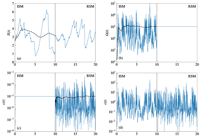
Figure 1: Temporal dynamics of different observables measured during typical runs of both the ISM (4) (left side of each panel) and the RSM with viscosity given by (7) (right side of each panel). On the x–axis of all panels time is measured in simulation units. Panels: (a) total energy $E$; (b) total enstrophy $\Omega$; (c) viscosity coefficient $\nu$; (d) energy dissipation rate $\varepsilon(t)=2\nu\Omega$. Continuous lines represent instantaneous values, dashed lines represent running averages (in time). For details on simulations, see Appendix A.1 and A.2.

Finally, the last term $f_{n}$ represents the forcing, which injects energy at an average rate $\langle\varepsilon\rangle=\langle\sum_{n}\mathcal{R}\{f_{n}u_{n}^{*}\}\rangle$, where $\mathcal{R}$ denotes the real part. In our simulations we considered a constant forcing, which preserves the time-reversal symmetry, acting only on the large scales (small wavenumbers) $f_{n}=f\delta_{n,0}$ with $f=const$.

2.2 Reversible shell model (RSM)

As discussed above the term $-\nu k_{n}^{2}u_{n}$ in Eq. (4) explicitly breaks the time reversal symmetry. In this section, we show how it can be modified by allowing the viscosity to vary depending on the velocity variables in such a way that the dynamics is (formally) time-reversible. In this way we can directly probe the irreversibility due the non-equilibrium energy cascade.

The first proposal to modify the Navier-Stokes equation in such a way to have a reversible dynamics is due to She and Jackson she1993constrained who introduced the constrained Euler equation, in order to devise a new Large Eddy Simulation (LES) scheme, by imposing a global constraint on the energy spectrum. On a more theoretical ground, Gallavotti gallavotti1996equivalence ; Gallavotti1997Dynamical proposed to modify the dissipative term by letting the viscosity depend on the velocity field in such a way to conserve a global quantity, e.g. energy or enstrophy. The value of these quantities is then determined by the initial conditions which should be taken so that the total energy or enstrophy, depending on the chosen constraint, equal the average value obtained from a long integration of the irreversible model dynamics. Gallavotti conjectured that these (formally) reversible equations should be “equivalent”, in the spirit of equivalence of ensembles in equilibrium statistical mechanics, to the (irreversible) NSE, at least in the limit of very high Reynolds number. This idea was then tested, for some aspects, in 2D NSE gallavotti2004lyapunov and, more recently, in the Lorenz 1996 model gallavotti2014equivalence , which can be thought as a single scale shell model.

Here we apply these ideas to the shell model (4). Past attempts to modify (4) imposing the energy conservation have encountered some difficulties in reproducing the dynamics of the original shell model Biferale1998 . When fixing the energy, we found similar difficulties. Briefly, the main problem is that, in the regime of energy cascade, the value of the mean energy is essentially determined at the integral (forcing) scales and is basically independent of the viscosity. Therefore, fixing the energy alone does not fix the extension of the inertial range (viz. the Reynolds number). On the other hand, fixing the enstrophy

$$\Omega=\sum_{n}k_{n}^{2}|u_{n}|^{2}\,$$ (5)

enforces a constraint on the small scales so that once its value is imposed via the initial condition the extension of the inertial range, and thus the Reynolds number, results well defined also in the reversible model. By using (4) in the request

$$\dot{\Omega}=0\,,$$ (6)

one obtains the dynamical evolution for the time-reversible viscosity

$$\nu_{R}(t) =\frac{\sum_{n}k_{n}^{2}\mathcal{R}\{f_{n}u_{n}^{*}\}}{\sum_{n}k_{n}^{4}|u_{n}|^{2}}+$$ (7)

$$+\frac{\sum_{n}\!k_{n}^{3}\!\left[a\lambda C_{3,n\!+\!1}\!+\!bC_{3,n}\!-\!\frac{c}{\lambda}C_{3,n\!-\!1}\right]}{\sum_{n}k_{n}^{4}|u_{n}|^{2}}\,,$$

where $C_{3,n}=-\mathcal{I}\{u_{n+1}u^{*}_{n}u^{*}_{n-1}\}$, and $\mathcal{I}$ stands for the imaginary part. It is worth noticing that there are two terms in the rhs of Eq. (7) because enstrophy is both injected by the forcing (first term) and produced by the nonlinear dynamics (second term). Most importantly, since $\nu_{R}$ is odd in the velocity variables, the modified dissipative term $-\nu_{R}k_{n}^{2}u_{n}$ preserves time reversal symmetry, i.e. does not change sign for $t\to-t$ and $u_{n}\to-u_{n}$.

Being $\nu_{R}$ a variable quantity, the initial condition for the $u_{n}$ becomes the only way of controlling the separation between the injection and dissipation scales in the system. Increasing the enstrophy of the initial condition increases the separation of scales and vice-versa. Further details on the simulation procedure can be found in the Appendices A.1 and A.2.

We conclude the presentation of the reversible shell model by showing, in Fig. 1, the time evolution of some global observables such as energy, enstrophy, energy dissipation and the viscosity itself measured both in the ISM and RSM. As one can see, in spite of the drastic change in the enstrophy and viscosity (Fig. 1b,c) the qualitative features of energy and energy dissipation are similar. The highly intermittent behavior of the energy dissipation, $\varepsilon(t)$, is qualitatively preserved in RSM. Notice that in the ISM the time-dependent energy dissipation reads $\varepsilon(t)=\nu\Omega(t)$ while in the RSM it takes the form $\varepsilon(t)=\nu_{R}(t)\Omega$, i.e. the quantity dependent on time is enstrophy in the former and the viscosity in the latter with the enstrophy $\Omega$ fixed at the average value obtained from the ISM. Also, the time average of the variable viscosity (7) is approximately equal to the value of $\nu$ in the corresponding irreversible simulation, which is a prerequisite to have the dynamical equivalence between the two dynamics gallavotti1996equivalence .

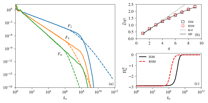
Figure 2: Comparison between the two models. (a) Structure function $F_{q}(k_{n})$ of order $q=2,4,6$ (as labeled) vs $k_{n}$, for the ISM (solid curves) and RSM (dashed curves). (b) Scaling exponents $\zeta(q)$ obtained by fitting the structure functions in the inertial range in the two models, compared with the K41 dimensional prediction ($q/3$) and the multifractal one (12), see legend. (c) Energy flux $\Pi^{E}_{n}$ as a function of the scale in both models. In all panels the error bars are smaller than the symbols. For details on the parameters of simulations see Appendix A.2 (parameter sets I1 and R1).

2.3 Lagrangian statistics in shell models

For shell models, lacking a spatial structure, there is not an obvious recipe for introducing a Lagrangian velocity. However, as observed in boffetta2002lagrangian , the quantity

$$v(t)=\sum_{n}\mathcal{R}\{u_{n}(t)\}$$ (8)

can be regarded as a sort of Lagrangian velocity. The choice of the real part is arbitrary, working with the imaginary part gives equivalent results.

The rationale for (8) is that the Lagrangian velocity is the superimposition of eddies at all scales, $u_{n}$ in the shell models. Since the shell model is not affected by sweeping bohr2005 , such a superposition is expected to reproduce the statistics of velocity along the particle path. Indeed it has been shown that $v(t)$ as defined above shares many qualitative and quantitative features of the Lagrangian velocity statistics of real 3D turbulent flows boffetta2002lagrangian . In particular, Lagrangian structure functions have been shown to display a scaling behavior with exponents deviating from the dimensional prediction and quantitatively close to those observed in experiments and simulations of the NSE mordant2001measurement ; chevillard2003lagrangian ; biferale2008lagrangian ; arneodo2008universal . Using (8) as a definition of Lagrangian velocity in the shell models, we define the Lagrangian acceleration as

$$a(t)=\dot{v}=\sum_{n}\mathcal{R}\{\dot{u}_{n}(t)\}\,,$$ (9)

and the Lagrangian power

$$p=va=\sum_{n}\mathcal{R}\{u_{n}\}\sum_{m}\mathcal{R}\{\dot{u}_{m}\}\,,$$ (10)

whose statistics can be studied in oder to explore the issue of Lagrangian time irreversibility.

We notice that the constant forcing on the first shell, which is used in our simulations, imposes a strong constraint on the phases of the first shells, leading to $\langle v(t)\rangle\neq 0$. Since, in principle, this may induce some spurious effects on the asymmetry of the power statistics, we have also tested our results with a (time-reversible) stochastic forcing for which the statistics of $v$ is symmetric around $\langle v(t)\rangle=0$, though non-Gaussian. Since the results we present are independent of the forcing choice, in the following we shall only show the constant forcing results, for a comparison with the other choice the reader may consult cencini2017time .

3 Energy cascade and anomalous scaling in the reversible shell model

The modified viscosity (7) can be interpreted within the framework of large eddy simulations as an effective model for small scale dissipation. In this respect it is worth mentioning that also for the NSE several time-reversible LES model have been proposed carati2001modelling ; fang2012time ; Jimenez2015 . It is thus important to verify whether and to what extent the RSM is able to reproduce the inertial range physics of the ISM. In particular, here, we study the scaling behavior of velocity structure functions that for shell models read jensen1991intermittency ; biferale2003shell ; bohr2005

$$F_{q}(k_{n})=\langle|u_{n}|^{q}\rangle\sim k_{n}^{-\zeta(q)}\,.$$ (11)

and the energy spectrum defined as $E_{n}\equiv F_{2}(k_{n})=\langle|u_{n}|^{2}\rangle$. For the standard Sabra shell model it has been shown Lvov_1998_improved_shellmodels that the exponents $\zeta(q)$ deviate from the dimensional (Kolmogorov 1941, K41) prediction, i.e. $\zeta(q)\neq q/3$, and are quantitatively close to the exponents of the Eulerian structure functions observed in experiments and simulations of the NSE.

In Fig. 2a, we compare the structure functions $F_{q}(k_{n})$ for $q=2,4$ and $6$ obtained from both ISM and RSM. As one can see their inertial-range scaling behavior is essentially indistinguishable. This is further confirmed in Fig. 2b where we compare the scaling exponents of the structure functions $\zeta(q)$ obtained by fitting the structure functions in both models. In Fig. 2b we also show that the scaling exponents are very well described by the multifractal formula (see Appendix B for a brief summary of the MF model for turbulence)

$$\zeta(q)=\inf_{h}\{hq+3-D(h)\}\,,$$ (12)

where for $D(h)$ we used a log-Poisson model [see Eq. (24)].

The constancy of the energy flux, $\Pi_{n}^{E}$, through the scale $k_{n}$, displayed in Fig. 2c, confirms that in both models a direct energy cascade is taking place. We remark, however, that the reversible shell model displays a slightly reduced inertial range, as inertial scaling disappears a few shells before its irreversible counterpart. A major difference between the two models is apparent in the dissipative range. Indeed the RSM shows a non trivial behavior at the scales where the ISM is exponentially damped by the fixed-viscosity dissipation.

3.1 Small scale behavior of the RSM

The reversible and irreversible shell models display different statistics at small scales, due to the different dissipative schemes. In the following we focus on this range of scales by looking at the energy and enstrophy spectra at varying the Reynolds number, i.e. the extension of the inertial range.

In the ISM, we observe an exponential suppression of turbulent fluctuations after the inertial range of scales, i.e. above the Kolmorogov wavenumber, $k_{\eta}\approx(\nu^{3}/\langle\varepsilon\rangle)^{-1/4}$. Conversely, in the RSM, we can distinguish an additional range of scales for $k>k_{\eta}$ characterized by a scaling close to a power law as clear from Fig. 3a, where we show the energy spectrum at increasing $\Omega$. At even larger wavenumbers, this power-law decay is followed by an exponential suppression, which is not visible in Fig. 3a due to the limited resolution but is clearly observed in simulations at smaller $\Omega$ (not shown).

As shown in Fig. 3b, the post-inertial range of scales shows a trend toward constancy of enstrophy at different $k_{n}$, suggesting equipartition of enstrophy and $E_{n}\sim k_{n}^{-2}$. Simulations at higher resolution (high $N$) and high values of $\Omega$ are computationally very demanding, due to the stiffness of ODE (4) and its numerical instability, so we were not able to explore higher values of $\Omega$ and determine unambiguously whether an effective equipartition of enstrophy is reached in the limit $\Omega\rightarrow\infty$. A further complication in understanding the physics of this range of scales is that both enstrophy equipartition and enstrophy cascade (constant flux) are characterized by the same energy spectrum scaling $E_{n}\sim k_{n}^{-2}$, making it difficult to predict the physical mechanism behind the observed dynamics from only looking at the spectrum. To disentangle the two possibilities, one would have to look at the enstrophy flux, however, at difference with $E$ or $H$, the enstrophy $\Omega$ is not an invariant for the non-linear term of equation (4), and its time-derivative cumulated on the first $M$ shells cannot be interpreted as a rate of transfer. In our simulations we found that the enstrophy dynamics is dominated by the balancing between the enstrophy generated by the non-linear interactions and the enstrophy dissipation.

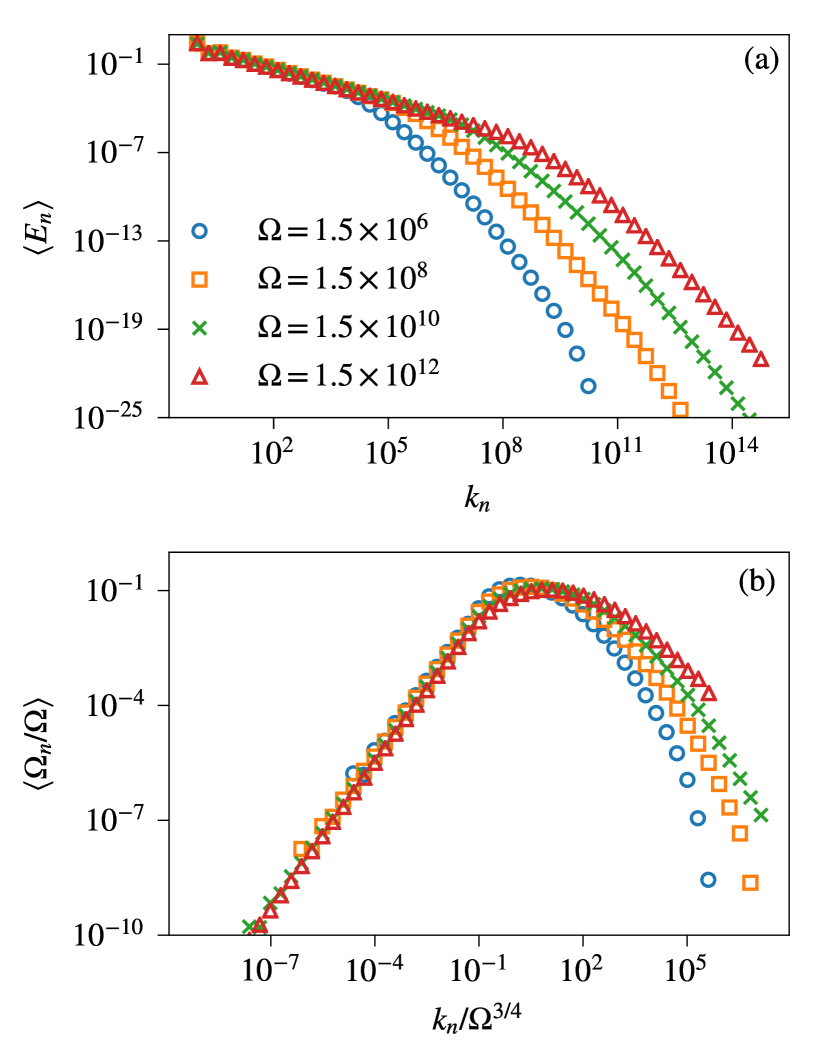
Figure 3: Energy (a) and enstrophy spectra (b) of the RSM at varying the total enstrophy $\Omega$. The enstrophy spectra in (b) have been rescaled in order to keep the Kolmogorov length-scale $O(1)$. Notice that in the RSM the Kolmogorov scale can be defined as $k_{\eta}\approx(\langle\nu\rangle^{3}/\langle\varepsilon\rangle)^{-1/4}\sim\langle\varepsilon\rangle^{-1/2}\Omega^{3/4}$, where we used that $\langle\nu\rangle=\langle\varepsilon\rangle/\Omega$. Errors, not shown, are of the same order of the symbol size or less. For details on simulations, see Appendix A (parameter sets R2-5).

Regardless of the underlying physical mechanism, the existence of a post-inertial range of scales suggests that the energy dissipation statistics of the RSM could be substantially different from that of the ISM. We thus studied the moments of the energy dissipation at varying the Reynolds number in both models. More specifically, we studied how the moments depend on the Taylor scale Reynolds number defined as $Re_{\lambda}=E/\sqrt{\nu\langle\varepsilon\rangle}$, i.e. as the ratio between the large scale time scale, $T_{L}=E/\langle\varepsilon\rangle$, and the small scale Kolmogorov time scale, $\tau_{\eta}=\sqrt{\nu/\langle\varepsilon\rangle}$. For the ISM, the moments of the energy dissipation are known to follow a power-law scaling on $Re_{\lambda}$ boffetta2000energy

$$\langle\varepsilon^{q}\rangle\sim Re_{\lambda}^{\chi(q)}$$ (13)

with the exponents $\chi(q)$ in agreement with the multifractal model as (see also Appendix B)

$$\chi(q)=\sup_{h}\left\{2\frac{D(h)-3-(3h-1)q}{1+h}\right\}\,,$$ (14)

where $D(h)$ is the same function used for the structure functions (12).

Since, in the RSM, the viscosity (7) can assume negative values, we studied the moments of the absolute value of the energy dissipation $\langle|\varepsilon|^{q}\rangle$ (we also checked that moments preserving the sign, such as $\langle|\varepsilon|^{q-1}\varepsilon\rangle$ give the same results, not shown). In Fig. 4 we show the exponents obtained by fitting the scaling behavior (13) for the moments of energy dissipation for both the RSM and ISM, together with the prediction (14). As one can see in the RSM the moments are definitely different from the ISM values, which are well predicted by (14). In particular, the exponents of the RSM are smaller, meaning that the intermittency of $\varepsilon$ is weaker in the reversible model.

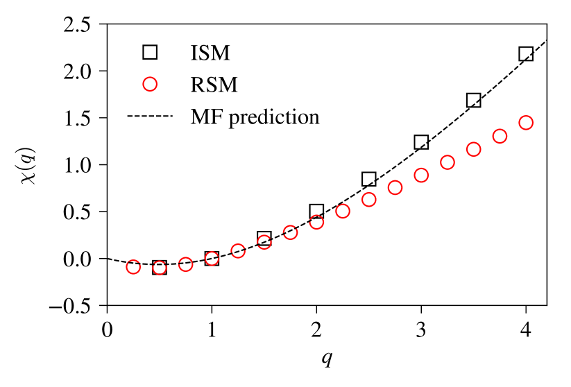
Figure 4: Scaling exponents of the moments of the energy dissipation (13) for the RSM (circles), and for the ISM (squares). The dashed line represents the MF prediction (14). Errors, not shown, are of the same order of the symbol size or less. For details on simulations, see Appendix A (parameter sets I2-9 and R6-14).

4 Lagrangian Power statistics and time irreversibility

It is useful to start this Section by briefly summarizing previous findings on Lagrangian power statistics in turbulence. As mentioned in the introduction, by inspecting both experimental and numerical trajectories of Lagrangian tracers Xu et al. xu2014 discovered that time increments of Lagrangian kinetic energy are negatively skewed and that this skewness persists for the time derivatives, i.e. for the Lagrangian power (3). Such skewness is directly linked to the time irreversibility of the tracer dynamics, as it means that the probability of gaining and losing kinetic energy is not the same, though $\langle p\rangle=0$ (by stationarity). In particular, they found that approximately:

$$\langle p^{2}\rangle\simeq\langle\varepsilon\rangle^{2}Re_{\lambda}^{4/3}\,,\quad\langle p^{3}\rangle\simeq-\langle\varepsilon\rangle^{3}Re_{\lambda}^{2}\,.$$ (15)

The above results convey two messages. First, the probability density function of $p$ is skewed, with $\langle p^{3}\rangle/\langle p^{2}\rangle^{3/2}\approx const<0$ suggesting that time-irreversibility is robust and persists in the limit $Re_{\lambda}\to\infty$. Second, the exponents $4/3$ and $2$, which approximately describe the scaling behavior of the second and third moment, strongly deviate from the dimensional prediction based on K41 theory, according to which

$$\langle p^{q}\rangle/\langle\varepsilon\rangle^{q}\propto Re_{\lambda}^{q/2}\,,$$ (16)

meaning that the Lagrangian power is strongly intermittent.

It has been shown, in cencini2017time , that the deviations from (16) can be understood within the framework of the multifractal model for turbulence (see also Appendix B). In particular, the MF model predicts that

$$\langle p^{q}\rangle\!\sim\!\langle\varepsilon\rangle^{q}Re_{\lambda}^{\alpha(q)}$$ (17)

with

$$\alpha(q)=\sup_{h}\left\{2\frac{(1-2h)q-3+D(h)}{1+h}\right\}\,.$$ (18)

In cencini2017time it is also shown that, defining the Lagrangian power as in (10), the (irreversible) shell model displays an intermittent statistics for $p$, but at variance with NS-turbulent data, deviations from the prediction (18) are present, at least in the statistical asymmetries of the power pdf. In this section, we broaden the investigation comparing Lagrangian power statistics in both the ISM and RSM.

4.1 Moments and asymmetry of Lagrangian power

For both the ISM and RSM the Lagrangian power is defined according to Eq. (10).

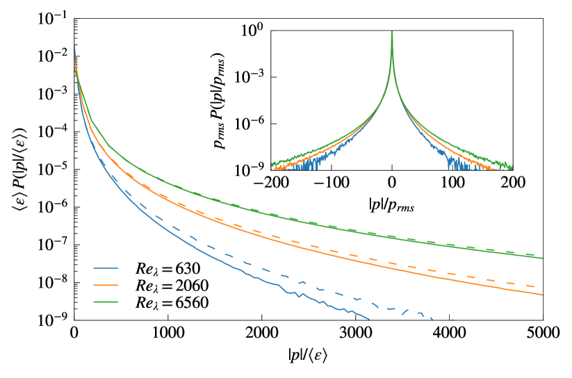
Figure 5: Probability density function of the Lagrangian power normalized by the average energy input rate, $p/\langle\varepsilon\rangle$, at three values of $Re_{\lambda}$ for the ISM. To highlight tail asymmetries, the pdf is plot against $|p|/\langle\varepsilon\rangle$, the positive/negative tail is in solid/dashed lines. Inset: the three pdfs of the main plot normalized with $p_{rms}=\langle p^{2}\rangle^{1/2}$, the curves do not overlap which is the signature of intermittency in the power statistics. For details on simulations, see Appendix A (parameter sets I4, I6, I8).

As discussed above, time irreversibility reveals itself in the odd order moments of the power that are sensitive to the asymmetries in the tails of the pdf of power. Such asymmetries are shown in Fig. 5 for different values of $Re_{\lambda}$. The absence of collapse onto a unique curve for the pdf of $p/\langle p^{2}\rangle^{1/2}$ (shown in the inset) highlights the presence of intermittency in the statistics of $p$. Here, following cencini2017time , in order to probe the scaling behavior of the symmetric and asymmetric component of the statistics we introduce two non-dimensional moments:

$$S_{q}=\frac{\langle|p|^{q}\rangle}{\langle\varepsilon\rangle^{q}};\quad A_{q}=\frac{\langle p|p|^{q-1}\rangle}{\langle\varepsilon\rangle^{q}}\,.$$ (19)

Clearly the latter vanishes for a symmetric (time-reversible) pdf.

Figure 6: Lagrangian power statistics in the ISM. Power moments $S_{q}$ and $-A_{q}$ (see legend) as a function of $Re_{\lambda}$ for (a) $q=2$ and (b) $q=3$. The curves for $-A_{q}$ have been shifted vertically to highlight the difference with respect to $S_{q}$. The black solid line shows the MF prediction (17)–(18). Panel (c): exponents for the $Re_{\lambda}$ dependence fitted from $S_{q}$ and $-A_{q}$ compared with K41 (16) and MF predictions (17)–(18). Inset: $Re_{\lambda}$-dependence of $\langle p/|p|\rangle\propto Re_{\lambda}^{-\mu}$ with $\mu\approx 0.187(7)$ as obtained by a best fit shown as a black line. Where error bars are not shown, it means that they are smaller or equal to the symbol size. For details on simulations, see Appendix A (parameter sets I2-9).

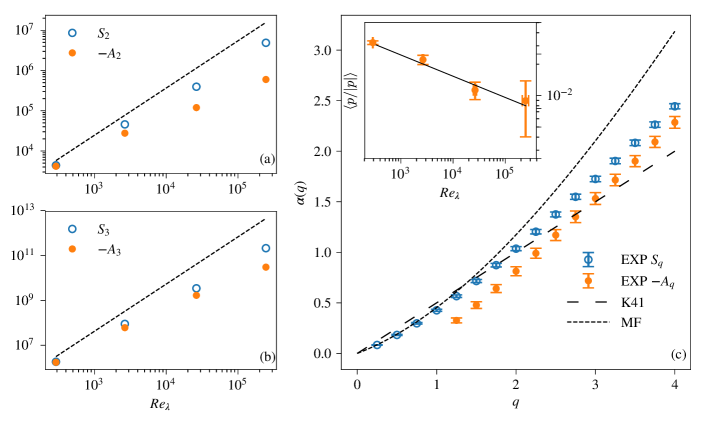
Figure 7: Lagrangian power statistics in the RSM. Panels (a), (b) and (c) present the same quantities as in Fig. 6 but for the RSM. Inset of panel (c): $Re_{\lambda}$-dependence of $\langle p/|p|\rangle\propto Re_{\lambda}^{-\mu}$ with $\mu\approx 0.20(7)$ as obtained by a best fit shown as a black line. For details on simulations, see Appendix A (parameter sets R2-5).

The main results on the Lagrangian power moments are summarized in Fig. 6 and Fig. 7 for the ISM and RSM, respectively. In Fig. 6a,b (Fig. 7a,b) we show the second and third moments for the ISM (RSM), respectively. Two observations are in order.

1. As for the ISM, the symmetric moments $S_{q}$ are in excellent agreement with the scaling behavior in $Re_{\lambda}$ predicted by the MF model obtained using (18) with the $D(h)$ given by (24) (see Fig. 2b). Conversely, deviations from the MF prediction are evident in the RSM.

2. For both models, the asymmetric moments $A_{q}$ are negative (positive) for $q>1$ ($q<1$) (we recall that $A_{1}=0$ by stationarity). The non-vanishing values of $A_{q}$ for $q\neq 0$ are the signature of time reversal symmetry breaking. In both models, the scaling behavior of $A_{q}$ is definitively different from that of $S_{q}$. In particular, the exponents are smaller and thus the asymmetry in the tails appears to be subleading with respect to the symmetric component.

The second observation implies that the generalized skewnesses $\tilde{S}_{q}=-A_{q}/S_{q}$, which measures the scaling ratio between the asymmetric and the symmetric components of the statistics at varying the order, are decreasing functions of $Re_{\lambda}$. This suggests that there is a statistical recovery of the time reversal symmetry in the limit of infinite $Re_{\lambda}$, at variance with what observed in NS turbulence xu2014 ; xu2014b ; cencini2017time . It is important to stress that the decay of the generalized skewness does not imply the decay of standard measures of skewness cencini2017time , such as e.g. $\langle p^{3}\rangle/\langle p^{2}\rangle^{1/2}$, which may be still growing with $Re_{\lambda}$ due to intermittency corrections, (see BV2001 for a similar issue in the problem of statistical recovery of isotropy).

Figure 6c (Fig. 7c) summarizes the results concerning the scaling exponents of the moments of power in the ISM (RSM). We can see the excellent agreement between the fitted exponents for $S_{q}$ of the ISM and the MF prediction. Strong deviations from the MF prediction are evident for the RSM, which is characterized by exponents smaller than predicted, denoting a less intermittent statistics. This behavior is consistent with the observation made for the energy dissipation (Fig. 4). This points to a major role played by the contribution of the dissipative terms to the Lagrangian power of shell models. To verify this, for the ISM, we decomposed the power in its contributions due to forcing, $p_{f}=v\sum_{n}\mathcal{R}\{f_{n}\}$, dissipation, $p_{d}=-v\nu\sum_{n}k_{n}^{2}\mathcal{R}\{u_{n}\}$, and nonlinear terms, $p_{nl}=v\sum\mathcal{R}\{ik_{n}(a\lambda u_{n+2}u^{*}_{n+1}+bu_{n+1}u^{*}_{n-1})\}$, where $p=p_{f}+p_{d}+p_{nl}$. We found that $\langle p_{d}^{2}\rangle/\langle p^{2}\rangle\approx 1$ and $\langle p_{nl}^{2}\rangle/\langle p^{2}\rangle\approx 2$ independently of $Re_{\lambda}$, which confirms that the dissipative and non-linear contributions scale as the total power and that they are of the same order. This is at odds with what has been observed in DNS of turbulent flows xu2014b , where the statistics is dominated by the pressure gradients, i.e. by the nonlinear terms, and the dissipative contribution was found to be subleading in terms of scaling and less intense with respect to the nonlinear one.

Figures 6c and 7c also show the exponents obtained by fitting the scaling behavior of the antisymmetric moments. For both ISM and RSM these exponents can be linked to the symmetric exponents by a rigid shift, i.e.

$$-A_{q}\sim S_{q}Re_{\lambda}^{-\mu}\,.$$ (20)

We found this relation to be consistent with the assumption that, in terms of scaling behavior, there is a decoupling between the absolute value of the power and its sign, i.e. $A_{q}\sim\langle p/|p|\rangle S_{q}$. Indeed for both models, as shown in the insets of Figs. 6c and 7c, we found

$$\langle p/|p|\rangle\sim Re_{\lambda}^{-\mu}\,,$$ (21)

with $\mu\approx 0.18$ ($0.2$) for the ISM (RSM). At present, this is just an observation of which we do not have a clear understanding. It should be remarked that the relation of (20) with (21) shows that the multifractal model is not completely failing in reproducing the asymmetries of the power statistics, and that the scaling behavior of the asymmetries is compatible, modulo the cancellation exponent $\mu$ (see also ott1992sign ), with the multifractal phenomenology. We emphasize that in DNS of the Navier-Stokes equations cencini2017time there is no evidence of a cancellation exponent different from zero, suggesting that the asymmetry persists also in the infinite Reynolds number limit.

5 Discussions and Conclusions

In this paper we have introduced a time-reversible shell model for turbulence, obtained by modifying the dissipative term of the so-called Sabra model, allowing the viscosity to vary in such a way as to maintain the total enstrophy constant. In spite of the formal time reversibility of the model we found that the dynamics spontaneously breaks the time reversal symmetry selecting an attractor onto which irreversibility manifests in the asymmetry of the Lagrangian power statistics.

A detailed quantitative comparison between the reversible and irreversible (original) shell models has shown that the dynamics of the former well reproduce the inertial range physics of the latter, indeed the structure functions of the two models are indistinguishable in the inertial range. On the contrary, the modified viscous term of the reversible model is responsible for important modifications in the physics below the Kolmogorov scale. While the irreversible model at these scales is characterized by an energy spectrum with an exponential fall-off, in the reversible model an intermediate range characterized by a close-to equipartition of enstrophy physics appears. The difference between the two models in this range of scale is responsible for a different statistics of the energy dissipation. As for the Lagrangian power statistics, we found that even though qualitatively the two models display the same features, quantitative details are different. In particular, the exponents characterizing the scaling behavior of the moments of power of the reversible model are smaller than those of the irreversible model. These differences are consistent with those observed for the energy dissipation and have, possibly, a similar origin in the non trivial physics of the reversible model below the Kolmogorov scale.

As for the irreversible shell model, consistently with our previous observations cencini2017time , we found that independently of the nature of the forcing, the (time-reversible) symmetric statistics of the power statistics are well captured by the multifractal model while deviations are present for the (time-irreversible) asymmetric component, which is characterized by smaller exponents. However, numerical evidence suggests that these deviations can be traced back to the Reynolds dependence of the sign of the power (cancellation exponent ott1992sign ). This indicates that the bulk part of the statistics is well captured by the multifractal model. Time-reversible sub-grid models for Large Eddy Simulations of the NSE might be important to better capture backscatter events where the energy is locally transferred from small to large scales in turbulence, i.e. when an inverse energy transfer is observed. The issue is particularly subtle considering that there is not a unique meaning of local energy transfer in the configuration space and that some of the inverse transfer events are probably simply due to large instantaneous fluctuations disconnected from any robust transfer mechanism chaodyn .

Authors contribution statement

All the authors conceived the study. MDP performed the simulations of RSM, MC performed simulations of the ISM. All the authors analyzed the data, discussed the results and wrote the manuscript.

Appendix A Details on simulations of RSM

A.1 General procedure for reversible simulations

In our simulations we always started by integrating equations (4) with constant viscosity over a time period long enough to guarantee stationarity of the dynamics and the convergence of the time averages of all the quantities measured.

Denoting with $\langle E_{n}\rangle|_{\nu}$ the average energy associated to the $n$-th shell of an irreversible shell-model simulation with constant viscosity $\nu$, we define the initial condition for the corresponding reversible simulation as

$$u_{n}(t=0)|_{\Omega}=[\langle E_{n}\rangle|_{\nu}]^{1/2}\,[\cos(\zeta_{n})+i\sin(\zeta_{n})]\,,$$ (22)

where the $\zeta_{n}$ are random angles. This definition guarantees that the reversible simulation will start with a total energy $E$ equal to the average energy of the corresponding irreversible run, and an enstrophy $\Omega$ (conserved in this case) equal to the average enstrophy of the corresponding irreversible run. For the irreversible simulations, the initial velocity field is chosen with random values on the first $6$ shells, and an initial energy $E(t=0)\sim 1$.

In all cases the time-integration algorithm we used is a modified fourth order Runge-Kutta scheme with explicit integration of the viscous term.

We averaged our measurements on an ensemble of $\sim 10$ simulations, differing in the choice of the initial conditions, for both the irreversible and the reversible models. In the reversible case, it is possible to build ensembles of simulations characterized by the same “Reynolds number” by picking different values for the $\zeta_{i}$ in (22), being the separation of scales effectively controlled by the ratio $\Omega/E$.

A.2 Parameters used

Here we report the sets of parameters used for the simulations presented in this paper. The I sets are for simulations of the ISM, the R sets are for simulations of the RSM. $N$ is the number of shells; $|f|$ is the magnitude of the forcing; $\nu$ is the value of the constant viscosity; $\Omega$ is the value of enstrophy; $dt$ is the integration timestep used; $T$ is the total time of integration, summed over all the simulations in the ensemble. The average energy and the big eddy turnover time are always $O(1)$.

set	$N$	$|f|$	$\nu$	$dt$	$T$
I1	$40$	$1$	$10^{-10}$	$2\times 10^{-8}$	$\sim 3000$
I2	$30$	$\sqrt{2}$	$10^{-4}$	$10^{-4}$	$\sim 10^{6}$
I3	$30$	$\sqrt{2}$	$3.16\times 10^{-5}$	$10^{-4}$	$\sim 10^{6}$
I4	$30$	$\sqrt{2}$	$10^{-5}$	$5\times 10^{-5}$	$\sim 10^{6}$
I5	$30$	$\sqrt{2}$	$3.16\times 10^{-6}$	$2.5\times 10^{-5}$	$\sim 10^{6}$
I6	$30$	$\sqrt{2}$	$10^{-6}$	$1.5\times 10^{-5}$	$\sim 10^{6}$
I7	$30$	$\sqrt{2}$	$3.16\times 10^{-7}$	$10^{-5}$	$\sim 10^{6}$
I8	$30$	$\sqrt{2}$	$10^{-7}$	$5\times 10^{-6}$	$\sim 10^{6}$
I9	$30$	$\sqrt{2}$	$3.16\times 10^{-8}$	$2.5\times 10^{-6}$	$\sim 10^{6}$

set	$N$	$|f|$	$\Omega$	$dt$	$T$
R1	$40$	$1$	$1.44\times 10^{10}$	$5\times 10^{-9}$	$\sim 720$
R2	$35$	$1$	$1.45\times 10^{6}$	$5\times 10^{-7}$	$\sim 12000$
R3	$45$	$1$	$1.44\times 10^{8}$	$5\times 10^{-8}$	$\sim 4500$
R4	$50$	$1$	$1.44\times 10^{10}$	$10^{-8}$	$\sim 720$
R5	$50$	$1$	$1.46\times 10^{12}$	$10^{-9}$	$\sim 405$
R6	$25$	$1$	$1.29\times 10^{4}$	$2\times 10^{-6}$	$\sim 130000$
R7	$25$	$1$	$4.38\times 10^{4}$	$2\times 10^{-6}$	$\sim 120000$
R8	$25$	$1$	$1.41\times 10^{5}$	$2\times 10^{-6}$	$\sim 190000$
R9	$35$	$1$	$4.29\times 10^{5}$	$5\times 10^{-7}$	$\sim 19000$
R10	$35$	$1$	$1.46\times 10^{6}$	$5\times 10^{-7}$	$\sim 10000$
R11	$35$	$1$	$4.26\times 10^{6}$	$5\times 10^{-7}$	$\sim 10000$
R12	$35$	$1$	$1.46\times 10^{7}$	$5\times 10^{-7}$	$\sim 8000$
R13	$45$	$1$	$4.30\times 10^{7}$	$5\times 10^{-8}$	$\sim 9000$
R14	$45$	$1$	$1.46\times 10^{8}$	$5\times 10^{-8}$	$\sim 3800$

Appendix B Multifractal model for Eulerian and Lagrangian statistics

Here we briefly recall the basic ideas on the multifractal model (MF) of turbulence FP1985 ; benzi1984multifractal ; frish_turbulence for the Eulerian statistics.

According to the MF model, Eulerian velocity increments at inertial scales are characterized by a local Hölder exponent $h$, i.e. $\delta_{r}u\sim U_{L}(r/L)^{h}$ ($L$ and $U_{L}$ denoting the large scale and the associated velocity, respectively), whose probability ${\cal P}(h)\sim r^{3-D(h)}$ depends on the fractal dimension $D(h)$ of the set where $h$ is observed. Thus the Eulerian structure functions can be written as

$$\langle(\delta_{r}u)^{q}\rangle\sim U_{L}^{q}\int_{h\in\mathcal{I}}dh\left(\frac{r}{L}\right)^{hq+3-D(h)}\sim U_{L}^{q}\left(\frac{r}{L}\right)^{\zeta(q)}\,,$$

where a saddle point approximation for $r\ll L$ gives

$$\zeta(q)=\inf_{h\in\mathcal{I}}\{hq+3-D(h)\}\,.$$ (23)

As for the Eulerian $D(h)$, in this paper we assume a Log-Poisson functional form she1994universal

$$D(h)=\frac{3(h-h_{0})}{\log(\beta)}\left[\log\left(\frac{3(h_{0}-h)}{d_{0}\log(\beta)}\right)-1\right]+3-d_{0}\,.$$ (24)

with $h_{0}=1/9$ and $d_{0}=(1-3h_{0})/(1-\beta)$ is fixed by imposing the exact relation $\zeta(3)=1$. For the shell model considered in this paper choosing $\beta=0.6$ one obtains an excellent fit for the scaling exponents of the structure functions (see Fig. 2).

In the MF framework, it is also possible to derive a prediction for the moments of the energy dissipation $\langle\varepsilon^{q}\rangle$ We can indeed estimate the (fluctuating) energy dissipation as $\varepsilon=(\delta_{\eta}u)^{3}/\eta$. According to the MF model $\eta=(\nu L^{h}/U_{L})^{1/(1+h)}$, and thus we have

$$\varepsilon=U_{L}^{4/(1+h)}\nu^{(3h-1)/(1+h)}L^{-4h/(1+h)}\,.$$ (25)

Then using the same procedure that led to (12) one can derive the scaling behavior of $\langle\varepsilon^{q}\rangle$ as a function of $Re_{\lambda}\sim\nu^{-1/2}$, namely

$${}\langle\varepsilon^{q}\rangle\sim Re_{\lambda}^{\chi(q)}\;\mathrm{with}\;\chi(q)=\sup_{h\in\mathcal{I}}\left\{2\frac{D(h)-3-(3h-1)q}{1+h}\right\}\,.$$ (26)

En passant notice that the $4/5$ law, namely the fact that $\zeta_{3}=1$ implies $\chi(1)=0$, i.e. the dissipative anomaly.

The multifractal model has been successfully extended to describe also several aspects of Lagrangian statistics, such as velocity borgas1993 ; boffetta2002lagrangian ; chevillard2003lagrangian ; arneodo2008universal , acceleration borgas1993 ; biferale2004 and Lagrangian power cencini2017time . Here we briefly recall the main steps.

To connect temporal velocity differences $\delta_{\tau}v$ over a time lag $\tau$, along fluid particle trajectories to equal time spatial velocity differences $\delta_{r}u$, in Refs.borgas1993 ; boffetta2002lagrangian it was noticed that $\delta_{\tau}v$ should receive the main contribution from eddies at a scale $r$ such that $\tau\sim r/\delta_{r}u$. This implies $\delta_{\tau}v\sim\delta_{r}u$ that establishes the bridge between Lagrangian and Eulerian quantities linking times and length scales:

$$\tau\sim T_{L}({r}/{L})^{1-h}$$ (27)

where $T_{L}=L/U_{L}$ is the eddy turnover time of the large scales. The bridging relation (27) provides a way to derive the expression for the scaling exponents of the Lagrangian structure function $S_{q}^{L}(\tau)=\langle(\delta_{\tau}v)^{q}\rangle\sim U_{L}^{q}(\tau/T_{L})^{\zeta_{L}(q)}$ with

$$\xi(q)=\inf_{h\in\mathcal{I}}\{[hq+3-D(h)]/(1-h)\}\,,$$ (28)

which with the same $D(h)$ used for the Eulerian statistics provides exponents in agreement with the shell model boffetta2002lagrangian and with experimental and DNS data of NS-turbulence chevillard2003 ; biferale2004 ; arneodo2008universal . In the same spirit, MF can be used to describe acceleration statistics noticing that $a\sim{\delta_{\tau_{\eta}}v}/{\tau_{\eta}}$, which yields biferale2004

$$a\sim\nu^{(2h-1)/(1+h)}U_{L}^{3/(1+h)}L^{-3h/(1+h)}\,.$$ (29)

The above expression, together with the definition of Lagrangian power, $p=av$ and recalling that $\nu\sim Re_{\lambda}^{-1/2}$, can be used to predict how the power moments $\langle p^{q}\rangle$ depend on $Re_{\lambda}$, which is cencini2017time

$$\langle p^{q}\rangle\!\sim\!\langle\varepsilon\rangle^{q}Re_{\lambda}^{\alpha(q)}$$ (30)

with

$$\alpha(q)=\sup_{h\in\mathcal{I}}\left\{2\frac{(1-2h)q-3+D(h)}{1+h}\right\}\,.$$ (31)

It is worth remarking that the scaling in $Re_{\lambda}$ is essentially carried by the acceleration, meaning that $\langle a^{q}\rangle\sim Re_{\lambda}^{\alpha(q)}$. In other terms a by product of the above analysis is that we should expect $\langle p^{q}\rangle\sim\langle a^{q}\rangle$ as far as scaling behavior is concerned.

We conclude noticing that, though asymmetries can be in principle introduced in the MF formalism (see, e.g., chevillard2012phenomenological ), the above derivations bear no information of statistical asymmetries in the statistics, therefore all the predictions should be understood as holding for the asymmetric components of the statistics, i.e. for the moments of the absolute values of the relevant quantities.

References

- (1) U. Frisch, Turbulence: The Legacy of A. N. Kolmogorov (Cambridge University Press, 1995)
- (2) C. De Lellis, L. Székelyhidi, Arch. Rat. Mech. Anal. 195(1), 225 (2010)
- (3) H. Rose, P. Sulem, J. Phys. (Paris) 39(5), 441 (1978)
- (4) G. Falkovich, K.R. Sreenivasan, Phys. Today 59(4), 43 (2006)
- (5) G. Gallavotti, Phys. Lett. A 223(1), 91 (1996)
- (6) G. Gallavotti, Physica D 105(1-3), 163 (1997)
- (7) G. Gallavotti, L. Rondoni, E. Segre, Physica D 187(1), 338 (2004)
- (8) G. Gallavotti, V. Lucarini, J. Stat. Phys. 156(6), 1027 (2014)
- (9) B. Sawford, P. Yeung, M. Borgas, Phys. Fluids 17(9), 095109 (2005)
- (10) J. Jucha, H. Xu, A. Pumir, E. Bodenschatz, Phys. Rev. Lett. 113(5), 054501 (2014)
- (11) L. Biferale, G. Boffetta, A. Celani, B. Devenish, A. Lanotte, F. Toschi, Phys. Fluids 17(11), 111701 (2005)
- (12) H. Xu, A. Pumir, G. Falkovich, E. Bodenschatz, M. Shats, H. Xia, N. Francois, G. Boffetta, Proc. Nat. Acad. Sci. 111(21), 7558 (2014)
- (13) A. Pumir, H. Xu, G. Boffetta, G. Falkovich, E. Bodenschatz, Phys. Rev. X 4(4), 041006 (2014)
- (14) M. Cencini, L. Biferale, G. Boffetta, M. De Pietro, Phys. Rev. Fluids 2(10), 104604 (2017)
- (15) T. Grafke, A. Frishman, G. Falkovich, Phys. Rev. E 91(4), 043022 (2015)
- (16) E. Piretto, S. Musacchio, F. De Lillo, G. Boffetta, Phys. Rev. E 94(5), 053116 (2016)
- (17) J. Wilson, B. Sawford, Bound.-Layer Meteor. 78(1), 191 (1996)
- (18) L. Biferale, Annu. Rev. Fluid Mech. 35(1), 441 (2003)
- (19) T. Bohr, M.H. Jensen, G. Paladin, A. Vulpiani, Dynamical systems approach to turbulence (Cambridge University Press, 2005)
- (20) U. Frisch, G. Parisi, in Turbulence and Predictability in Geophysical Fluid Dynamics and Clim ate Dynamics, ed. by U. M. Ghil (North–Holland, 1985)
- (21) R. Benzi, G. Paladin, G. Parisi, A. Vulpiani, J. Phys. A: Math. Gen. 17(18), 3521 (1984)
- (22) Z.S. She, E. Jackson, Phys. Rev. Lett. 70(9), 1255 (1993)
- (23) D. Carati, G. Winckelmans, H. Jeanmart, J. Fluid Mech. 441, 119 (2001)
- (24) L. Fang, W. Bos, L. Shao, J.P. Bertoglio, J. Turb. (13), N3 (2012)
- (25) A. Vela-Martín, J. Jiménez, (2015). Reversibility in the 3D inertial turbulent cascade, extended abstract presented at the Conference ETC15, 15th European Turbulence Conference, Delft, The Netherlands, 25-28 August,2015, http://www.etc15.nl/proceedings/proceedings/documents/403.pdf.
- (26) P. Ditlevsen, Turbulence and shell models (Cambridge University Press, 2010)
- (27) V. L’vov, E. Podivilov, A. Pomyalov, I. Procaccia, D. Vandembroucq, Phys. Rev. E 58, 1811 (1998)
- (28) E. Gledzer, Dokl. Akad. Nauk SSSR 209(5), 1046 (1973)
- (29) K. Ohkitani, M. Yamada, Prog. Theor. Phys. 81(2), 329 (1989)
- (30) M. Jensen, G. Paladin, A. Vulpiani, Phys. Rev. A 43(2), 798 (1991)
- (31) L. Biferale, D. Pierotti, A. Vulpiani, J Phys. A: Math. and Gen. 31(1), 21 (1998)
- (32) G. Boffetta, F. De Lillo, S. Musacchio, Phys. Rev. E 66(6), 066307 (2002)
- (33) N. Mordant, P. Metz, O. Michel, J.F. Pinton, Phys. Rev. Lett. 87(21), 214501 (2001)
- (34) L. Chevillard, S. Roux, E. Lévêque, N. Mordant, J.F. Pinton, A. Arnéodo, Phys. Rev. Lett. 91(21), 214502 (2003)
- (35) L. Biferale, E. Bodenschatz, M. Cencini, A. Lanotte, N. Ouellette, F. Toschi, H. Xu, Phys. Fluids 20(6), 065103 (2008)
- (36) A. Arnéodo, et al., Phys. Rev. Lett. 100(25), 254504 (2008)
- (37) G. Boffetta, A. Celani, D. Roagna, Phys. Rev. E 61, 3234 (2000)
- (38) L. Biferale, M. Vergassola, Phys. Fluids 13(8), 2139 (2001)
- (39) E. Ott, Y. Du, K. Sreenivasan, A. Juneja, A. Suri, Phys Rev. Lett. 69(18), 2654 (1992)
- (40) M. Buzzicotti, M. Linkmann, H. Aluie, L. Biferale, J. Brasseur, C. Meneveau, arXiv:1706.03219 (2017)
- (41) Z.S. She, E. Leveque, Phys. Rev. Lett. 72(3), 336 (1994)
- (42) M. Borgas, Philos. Trans. 342(1665), 379 (1993)
- (43) L. Biferale, G. Boffetta, A. Celani, B. Devenish, A. Lanotte, F. Toschi, Phys. Rev. Lett. 93(6), 064502 (2004)
- (44) L. Chevillard, S. Roux, E. Lévêque, N. Mordant, J.F. Pinton, A. Arnéodo, Phys. Rev. Lett. 91(21), 214502 (2003)
- (45) L. Chevillard, B. Castaing, A. Arneodo, E. Lévêque, J.F. Pinton, S. Roux, Comp. Rend. Phys. 13(9-10), 899 (2012)