X-Ray Observations of Magnetar SGR 0501+4516 from Outburst to Quiescence

Abstract

Magnetars are neutron stars having extreme magnetic field strengths. Study of their emission properties in quiescent state can help understand effects of a strong magnetic field on neutron stars. SGR 0501+4516 is a magnetar that was discovered in 2008 during an outburst, which has recently returned to quiescence. We report its spectral and timing properties measured with new and archival observations from the Chandra X-Ray Observatory, XMM-Newton, and Suzaku. We found that the quiescent spectrum is best fit by a power-law plus two blackbody model, with temperatures of $kT_{\rm low}\sim 0.26\,{\rm keV}$ and $kT_{\rm high}\sim 0.62\,{\rm keV}$. We interpret these two blackbody components as emission from a hotspot and the entire surface. The hotspot radius shrunk from $1.4\,{\rm km}$ to $0.49\,{\rm km}$ since the outburst, and there was a significant correlation between its area and the X-ray luminosity, which agrees well with the prediction by the twisted magnetosphere model. We applied the two-temperature spectral model to all magnetars in quiescence and found that it could be a common feature among the population. Moreover, the temperature of the cooler blackbody shows a general trend with the magnetar field strength, which supports the simple scenario of heating by magnetic field decay.

1. Introduction

Magnetars are non-accreting neutron stars with long spin periods ($P\sim 2$–$12\,{\rm s}$) and the largest spin-down rates ($\dot{P}\sim 10^{-13}$–$10^{-10}\,{\rm s}\,{\rm s}^{-1}$) among the pulsar population. Most of them have spin-down inferred magnetic field strength, $B$, up to $\sim 10^{15}\,{\rm G}$. It is generally believed that magnetars are young neutron stars and some are found inside Supernova Remnants (SNRs). Magnetars usually have persistent X-ray luminosity, $L_{\rm X}\sim 10^{34-36}\,{\rm erg}\,{\rm s}^{-1}$, much larger than their rotational energy loss rate $\dot{E}$, and they occasionally exhibits violent bursting activities (see review by Kaspi & Beloborodov, 2017). In order to explain the properties of this pulsar class, magnetar models have been developed. The most popular one is the twisted magnetosphere model (Thompson & Duncan, 1995, 2001; Beloborodov, 2009, 2011). It suggests that the toroidal magnetic field could exist in the stellar crust. If the internal magnetic field is strong enough, it could tear the crust followed by twisting the crust-anchored external field (Thompson & Duncan, 1995; Thompson et al., 2000, 2002). In addition, a starquake arising from the plastic deformation of the crust would cause magnetar bursts due to magnetic reconnection (Thompson & Duncan, 1995; Parfrey et al., 2012, 2013). Persistent X-ray emission of magnetars could be explained by the magnetic field decay (Thompson et al., 2002; Pons et al., 2007). Meanwhile, the magneto-thermal evolution theory suggests that the field decay could be enhanced due to the changes in the conductivity and the magnetic diffusivity of magnetars (Viganò et al., 2013). As a consequence, magnetars are observed to have higher surface temperature and X-ray luminosity than canonical pulsars. In general, soft X-ray spectra of magnetars can be described by an absorbed blackbody model with temperature $kT\sim 0.3$–$0.6\,{\rm keV}$ plus an additional power-law with photon index $\Gamma\sim 2$–$4$ or another blackbody component with $kT\sim 0.7\,{\rm keV}$ (see Olausen & Kaspi, 2014; Kaspi & Beloborodov, 2017). It indicates that the soft X-ray emission could be contributed by thermal emission and some non-thermal radiation processes, such as synchrotron or inverse-Compton scattering.
SGR 0501+4516 (catalog ) is a magnetar discovered with the Burst Alert Telescope (BAT) on board Swift on 2008 August 22 due to a series of short bursts (Barthelmy et al., 2008). X-ray pulsations were detected with a period of $P\sim 5.7\,{\rm s}$ (Rea et al., 2009). After the discovery, the source was subsequently identified in an archival ROSAT observation taken in 1992. The soft X-ray flux was $\sim 80$ times higher in the outburst when compared to the 1992 observation (Rea et al., 2009). The hard X-ray tail above $10\,{\rm keV}$ was first discovered with INTEGARL right after the outburst (Rea et al., 2009). It had also been detected with Suzaku observation (Enoto et al., 2010). From the spin period and spin-down rate, $B$ was estimated to be $2\times 10^{14}\,{\rm G}$ (Woods et al., 2008). The soft X-ray spectrum of SGR 0501+4516 below $10\,{\rm keV}$ could be described by an absorbed blackbody model with a power-law component, using XMM-Newton observations obtained in the first year after the outburst (Rea et al., 2009; Camero et al., 2014). The X-ray spectral properties from 2008 to 2013 were also measured with four Suzaku observations (Enoto et al., 2017), but it is interesting to note that the results are different from those reported in other literature, including a smaller hydrogen column density, lower blackbody temperature, larger radius, and softer power-law photon index (Rea et al., 2009; Göǧüş et al., 2010; Camero et al., 2014).

Table 1Observations of SGR 0501+4516 Used in Our Analysis.

Date	Observatory (Instruments)	ObsID	Mode	Net Exposure (ks)
2008 Aug 31	XMM-Newton (PN)	0552971201	SW	$10.2$
2008 Sep 02	XMM-Newton (PN)	0552971301	SW	$20.5$
2008 Sep 25	CXO (HRC-I)	9131	–	$10.1$
2008 Sep 30	XMM-Newton (PN/MOS1/MOS2)	0552971401	LW/SW/SW	$30.1/32.3/32.3$
2009 Aug 30	XMM-Newton (PN/MOS1/MOS2)	0604220101	SW/FF/SW	$53.9/52.4/53.1$
2012 Dec 09	CXO (ACIS-S)	15564	TE	$14.0$
2013 Apr 03	CXO (ACIS-S)	14811	TE	$13.7$
2013 Aug 31	Suzaku (XIS0/XIS1/XIS3)	408013010	Normal	$36.0/41.1/41.2$

Note. —

Until now, there is no accurate distance measurement for SGR 0501+4516. As magnetars are young pulsars, SGR 0501+4516 is expected to be located close to the spiral arm of the Galaxy. The line of sight intercepts the Perseus and Outer arms of the Galaxy, at distances of $\sim 2.5$ and $\sim 5\,{\rm kpc}$, respectively. In this paper, we assume the distance $d=5\,{\rm kpc}$. In addition, there exists a supernova remnant (SNR) G160.9+2.6, $\sim 80^{\prime}$ north of SGR 0501+4516 (Gaensler & Chatterjee, 2008; Göǧüş et al., 2010). The distance and age of the SNR were estimated as $800\pm 400\,{\rm pc}$ and $4000$–$7000\,{\rm years}$ (Leahy & Tian, 2007). Göǧüş et al. (2010) proposed that SGR 0501+4516 could be associated with G160.9+2.6. Leaving the distance aside, if this is the case, the magentar should have a large proper motion of $0\farcs 7$–$1\farcs 2\,{\rm yr}^{-1}$ to the south.
In this paper, we used new X-ray observations to show that SGR 0501+4516 had returned to quiescence in 2013, five years after the outburst, and we report on its spectral and timing properties during flux relaxation. We also analyzed archival observations to investigate the long-term evolution.

2. Observations and data reduction

There are eight X-ray observations used in this study (see Table 1). We obtained two new observations obtained with the Advanced CCD Imaging Spectrometer (ACIS) on board Chandra X-ray Observatory (CXO) on 2012 December 9 and 2013 April 3. Both of them were made in the Time Exposure (TE) mode for 14 ks using only one-eighth of the CCD, providing a fast frame time of 0.4 s. This allows us to obtain a crude pulse profile for this $\sim 5.67\,{\rm s}$ period pulsar. By inspecting the light curves, no bursts from the source or background flares were detected during the exposures. We checked that pile-up was negligible in both observations. In addition to these two ACIS observations, a Chandra High Resolution Camera (HRC) observation taken on 2008 September 25 was also used to measure the source position only. All Chandra data were reprocessed with chandra_repro in CIAO 4.8 with CALDB 4.7.4 before performing any analysis.
There were six XMM-Newton observations after the discovery of the source. We only analyzed the latest four from 2008 August 31 to 2009 August 30 because SGR 0501+4516 showed strong bursting activities during the two earliest observations. The source was still bright 11 days after the outburst; the pile-up effect was an issue in the MOS data obtained on 2008 August 31 and September 2 and hence only the PN data were used in these two observations. We first reprocessed all the data by the tasks epchain/emchain in XMMSAS version 1.2. In the analysis, only PATTERN $\leq 4$ events of the PN data and PATTERN $\leq 12$ events in the MOS data were used. We also used the standard screening for the MOS (FLAGS = #XMMEA_EM) and PN (FLAGS = #XMMEA_EP) data. After removal of periods with background flares, we obtained net exposures ranging from $10.2$ to $53.9\,{\rm ks}$ (see Table 1).
We also used the latest Suzaku data in the archive taken on 2013 August 31, to combine with the Chandra data to better constrain the quiescent spectral properties. In order to focus on the soft X-ray spectral properties, only the data obtained with the XIS were used (see Table 1). The XIS data were reprocessed using xisrepro in HEAsoft 6.20 with standard screening criteria. We inspected the light curves to verify that no bursts were detected throughout the observation with $\sim 40\,{\rm ks}$.

3. ANALYSIS AND RESULTS

3.1. Imaging and Astrometry

We measured the position of SGR 0501+4516 in all Chandra data using the task celldetect and obtained a consistent result of $\alpha$=5:01:06.8, $\delta$=+45:16:34 (J2000) within the uncertainty. The measurement uncertainties in the $90\%$ confidence level have radii $0\farcs 4$ (HRC) and $0\farcs 5$ (ACIS). As the ACIS images were taken in the sub-array mode with a small field of view, we did not find any background sources to align the two images. Therefore, we also need to consider the absolute astrometric accuracy of Chandra, which is $0\farcs 8$ at the $90\%$ confidence level. This gives an upper limit of the proper motion of $0\farcs 32\,{\rm yr}^{-1}$ ($90\%$ confidence level), rejecting the suggestion that SGR 0501+4516 was born at the center of SNR G160.9+2.6 (Göǧüş et al., 2010).
Finally, we simulated a model point spread function for ACIS data with ChaRT using the best-fit spectrum (see Section 3.3 below) and confirmed that the radial profile is fully consistent with that of the real data, indicating no extended emission was found near the magnetar.

3.2. Timing Analysis

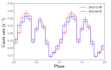
Figure 1.— Pulse profiles of SGR 0501+4516 in the energy range of $0.5$–$7\,{\rm keV}$ for the latest Chandra observations. The two profiles were aligned manually by matching the brightest bin. The uncertainties are at the $1\sigma$ level.

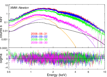
Figure 2.— XMM-Newton PN spectra of SGR 0501+4516. The solid lines indicate the best-fit 2BB+PL model on different epochs. The orange, purple, and black dashed lines indicate the low temperature BB, high temperature BB, and PL components of the 2009 August 30 spectrum, respectively.

Figure 3.— Chandra and Suzaku spectra of SGR 0501+4516. All solid lines indicate the same best-fit 2BB+PL model. The different shape is due to different responses of the instruments. The orange, purple, and black dashed lines indicate the low temperature BB, high temperature BB, and PL components, respectively, with the Suzaku XIS response.

We extracted the source photons from the two new Chandra observations by using a $2\farcs 5$ radius aperture and obtained 4149 and 4043 counts, respectively, in the $0.5$–$7\,{\rm keV}$ energy range. The estimated background photon counts in the source region are $\sim 0.6$ for both observations. We then applied a barycentric correction to the photon arrival times. We employed the $\chi^{2}$-test after epoch folding (Leahy, 1987) and found periods of $P=5.76286(8)\,{\rm s}$ and $P=5.76299(9)\,{\rm s}$ for 2012 December 9 and 2013 April 3 data, respectively. The $1\sigma$ uncertainties quoted here were estimated using the simulation results from Leahy (1987). We used the best-fit periods to generate the pulse profiles for both Chandra observations. As the frame time of our observations was $0.4\,{\rm s}$, we only divided the pulse period of $P=5.76\,{\rm s}$ into 13 phase bins. Figure 1 shows the pulse profile, which has a double-peaked shape. The pulse profile between the two observations did not show any obvious variations, suggesting that the source had already returned to quiescence in 2013.
As the dates of the two new Chandra observations were separated by too far apart, we were unable to measure the spin-down rate $\dot{P}$ by phase coherent timing analysis. Meanwhile, the uncertainties of individual timing measurements were too large so that $\dot{P}$ could not be obtained from our Chandra observations. We found that the two periods measured in 2012 and 2013 are formally consistent with each other after accounting for the uncertainties; however, they are different from the value obtained in the 2009 observation (Camero et al., 2014). Comparing our results with the spin period $P=5.7622571(2)$ measured in 2009, we obtained $\dot{P}=6(1)\times 10^{-12}\,{\rm s}\,{\rm s}^{-1}$ at the $1\sigma$ confidence level from 2009 to 2013, which is compatible with $5.94(2)\times 10^{-12}\,{\rm s}\,{\rm s}^{-1}$ reported by Camero et al. (2014).

3.3. Spectral Analysis

We extracted the source spectrum from the Chandra observations using the same $2\farcs 5$ radius apertures as in the timing analysis above. For the XMM-Newton and Suzaku XIS spectra, we used apertures of $36^{\prime\prime}$ and $1\farcm 8$ radius, respectively. We chose a larger region far from the source on the same CCD as the background region. We restricted the analysis in the energy range of $0.5$–$10\,{\rm keV}$ for XMM-Newton and Suzaku data, and $0.5$–$7\,{\rm keV}$ for Chandra data to optimize the signal-to-noise ratio. We grouped the spectra with a minimum of 30 counts per energy bin.

Table 2Best-Fit Spectral Parameters for SGR 0501+4516 with Uncertainties at the $90\%$ Confidence Level

Date	$N_{\rm H}$	$kT_{\rm low}$	$R_{\rm low}$	$F_{\rm low}$ ($10^{-11}$	$kT_{\rm high}$	$R_{\rm high}$	$F_{\rm high}$ ($10^{-11}$	$\Gamma$	$F_{\rm PL}$ ($10^{-11}$	$\chi^{2}/{\rm dof}$
	$(10^{22}\,{\rm cm}^{-2})$	(keV)	(km)	erg cm${}^{-2}\,{\rm s}^{-1}$)	(keV)	(km)	${\rm erg}\,{\rm cm}^{-2}\,{\rm s}^{-1}$)		erg cm${}^{-2}\,{\rm s}^{-1}$)
BB+PL model
2008 Aug 31	$1.34\pm 0.06$	$\cdots$	$\cdots$	$\cdots$	$0.70\pm 0.02$	$1.45_{-0.08}^{+0.09}$	$1.48\pm 0.08$	$2.9\pm 0.1$	$1.63\pm 0.08$	$764.9/741$
2008 Sep 02	$1.29_{-0.05}^{+0.04}$	$\cdots$	$\cdots$	$\cdots$	$0.68\pm 0.01$	$1.46\pm 0.06$	$1.34\pm 0.05$	$2.85\pm 0.07$	$1.46\pm 0.06$	$947.0/915$
2008 Sep 30	$1.36\pm 0.03$	$\cdots$	$\cdots$	$\cdots$	$0.66\pm 0.01$	$1.03\pm 0.04$	$0.57\pm 0.02$	$3.15_{-0.05}^{+0.06}$	$0.87\pm 0.02$	$2367.5/2169$
2009 Aug 30	$1.43\pm 0.04$	$\cdots$	$\cdots$	$\cdots$	$0.56\pm 0.02$	$0.56\pm 0.05$	$0.072_{-0.007}^{+0.008}$	$4.0\pm 0.1$	$0.21\pm 0.01$	$1308.3/1227$
2013 Jun 23	$1.43_{-0.08}^{+0.09}$	$\cdots$	$\cdots$	$\cdots$	$0.63_{-0.05}^{+0.04}$	$0.34_{-0.05}^{+0.06}$	$0.05\pm 0.01$	$3.9_{-0.2}^{+0.3}$	$0.15\pm 0.01$	$626.9/603$
2BB+PL model
2008 Aug 31	$0.90\pm 0.02$	$0.35_{-0.02}^{+0.03}$	$4.6_{-0.5}^{+0.6}$	$0.55\pm 0.09$	$0.75\pm 0.02$	$1.4\pm 0.1$	$2.14_{-0.09}^{+0.07}$	$1.33\tablenotemark{g}$	$0.42\pm 0.07$	$5911.5/5653$
2008 Sep 02	$0.90\pm 0.02$	$0.31\pm 0.02$	$5.2_{-0.6}^{+0.7}$	$0.38\pm 0.05$	$0.71_{-0.02}^{+0.01}$	$1.56_{-0.06}^{+0.10}$	$1.99_{-0.05}^{+0.04}$	$1.33\tablenotemark{g}$	$0.45\pm 0.04$	$5911.5/5653$
2008 Sep 30	$0.90\pm 0.02$	$0.31\pm 0.01$	$4.8_{-0.2}^{+0.4}$	$0.30\pm 0.02$	$0.69_{-0.01}^{+0.02}$	$1.13_{-0.06}^{+0.05}$	$0.95\pm 0.02$	$1.33\tablenotemark{g}$	$0.20\pm 0.02$	$5911.5/5653$
2009 Aug 30	$0.90\pm 0.02$	$0.25\pm 0.02$	$4.4_{-0.4}^{+0.8}$	$0.085\pm 0.008$	$0.56_{-0.02}^{+0.06}$	$0.7\pm 0.1$	$0.14\pm 0.01$	$2.6_{-2.5}^{+0.4}$	$0.06_{-0.02}^{+0.01}$	$5911.5/5653$
2013 Jun 23	$0.90\pm 0.02$	$0.26_{-0.02}^{+0.01}$	$3.7_{-0.7}^{+0.3}$	$0.07\pm 0.01$	$0.62_{-0.04}^{+0.03}$	$0.49_{-0.10}^{+0.05}$	$0.10_{-0.02}^{+0.01}$	$2.3_{-2.5}^{+0.7}$	$0.032_{-0.025}^{+0.012}$	$5911.5/5653$

Note. —

All spectral analyses were performed in the Sherpa environment. We tried an absorbed blackbody plus power-law (BB+PL) model as in previous studies (Rea et al., 2009; Göǧüş et al., 2010; Camero et al., 2014). We used the interstellar absorption model tbabs and the solar abundances were set to wilm (Wilms et al., 2000). The XMM-Newton spectra from the same epoch were fit with a single set of parameters. We found that the Chandra and Suzaku spectra share similar best-fit parameters, suggesting the quiescent property. In order to boost the signal-to-noise ratio, we fit them together with the same parameters.

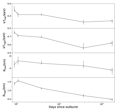
Figure 4.— Evolution trends for the best-fit parameters of SGR 0501+4516 with the 2BB+PL model since the 2008 outburst.

The best-fit spectral parameters are listed in Table 2. From 2008 to 2013, the best-fit blackbody radius shrunk significantly from $R=1.45\,{\rm km}$ to $R=0.34\,{\rm km}$ (assuming $d=5\,{\rm kpc}$) and the power-law photon index softened from $\Gamma=2.9$ to $\Gamma=3.9$. Our XMM-Newton results are consistent with those reported by Rea et al. (2009) and Camero et al. (2014) except with a slightly higher absorption column density $N_{\rm H}$ due to the different absorption model we used. While Camero et al. (2014) suggested that the source had already returned to its quiescence one year after the 2008 outburst, our new results show that the total absorbed flux was still decreasing from $2.8\times 10^{-12}\,{\rm erg}\,{\rm cm}^{-2}\,{\rm s}^{-1}$ in 2009 to $2.0\times 10^{-12}\,{\rm erg}\,{\rm cm}^{-2}\,{\rm s}^{-1}$ in 2013. Comparing with the previously reported Suzaku results, our blackbody component has a higher temperature and smaller size. This could be the result of the much lower column density ($N_{\rm H}\sim 0.4\times 10^{22}\,{\rm cm}^{-2}$) reported by Enoto et al. (2017).
We noted the best-fit PL component is soft with $\Gamma\gtrsim 3$. This could indicate the thermal nature of the emission. To verify that, we tried to narrow down the energy range to $6\,{\rm keV}$ and compared the best-fit results of the BB+PL and the double-blackbody (2BB) models. We found that the latter provided better fits to all spectra, thus, confirming our idea. When we fit the entire energy range, the 2BB fit has obvious residuals in the highest energy bins for all XMM-Newton spectra, hinting at an additional PL component. In the final model, we consider the double-blackbody plus power-law (2BB+PL) model and found that it provides the best fit. Assuming that $N_{\rm H}$ remained unchanged between epochs, we fit all spectra simultaneously with a linked absorption model. We found that the PL component dominated only above $\sim 6\,{\rm keV}$ for which our observations were not very sensitive. As the first three XMM-Newton observations were taken within $\sim 1$ month after the 2008 August 26 Suzaku observation, we believe that they should share a similar spectral property. In order to obtain a better fit, we adopted the 2BB+PL result reported by Enoto et al. (2010) and fixed $\Gamma=1.33$ in the fitting of the 2008 XMM-Newton spectra. As the photon index could have changed after 2008, we did not fix $\Gamma$ for all spectra taken after 2009. However, the PL component was poorly constrained. We list the best-fit spectral results in Table 2. The best-fit 2BB+PL model to the XMM-Newton PN spectra at different epochs are plotted in Figure 3, and the fit to the last epoch Chandra and Suzaku spectra are plotted in Figure 3. Figure 4 shows evolution trends of the two blackbody components. The temperature of the cooler blackbody component dropped from $kT_{\rm low}=0.35\,{\rm keV}$ in 2008 to $0.26\,{\rm keV}$ in 2012, while there was no significant change in the radius, with $R_{\rm low}$ stayed $\sim 4.5\,{\rm km}$ among all the observations. The best-fit parameters for the hotter blackbody component, meanwhile, are consistent with those from the BB+PL fit. Both the temperature $kT_{\rm high}$ and the radius $R_{\rm high}$ of this component dropped since the outburst. We found that adding the best-fit ${\rm BB}_{\rm high}$ component shares similar parameters as the ${\rm BB}_{\rm high}$ in the BB+PL model. Similar to the BB+PL results, Figure 4 shows that $R_{\rm high}$ was not lowest in 2009, indicating that the source was not yet in quiescence at that time.

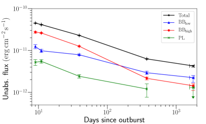
Figure 5.— Decay trends of unabsorbed fluxes of SGR 0501+4516 for all components in the 2BB+PL model.

In Figure 5, we plot the flux evolution of all components in the 2BB+PL model, we see decreasing trends since the 2008 outburst. The plot indicates a significant drop of the ${\rm BB}_{\rm high}$ flux after 2009, and we claim that the source had not yet returned to quiescence at that time. On the other hand, we found similar count rates in the 2012 and 2013 Chandra observations, which suggests that SGR 0501+4516 had reached a quiescent state five years after the outburst. Finally, we note that there is no obvious plateau in the flux evolution, contrary to what the crustal cooling model suggests (Lyubarsky et al., 2002).
In addition to the BB+PL and 2BB+PL models, we also tried the resonant cyclotron scattering (RCS) (Rea et al., 2008) and the 3D surface thermal emission and magnetospheric scattering (STEM3D) models (Weng & Göğüş, 2015) but the fits converged to the boundary of the parameter space. Therefore, we do not believe that the results are physical.

Table 3Two-Temperature Fits to the Spectra of Magnetars in Quiescence with Uncertainties or Upper Limits at the $90\%$ Confidence Level

Object	Instrument (ObsID)	Model	$N_{\rm H}$	$kT_{\rm low}$	$R_{\rm low}$	$kT_{\rm high}$	$R_{\rm high}$	$\Gamma$	$\chi^{2}_{\nu}$ (dof)
			$(10^{22}\,{\rm cm}^{-2})$	(keV)	(km)	(keV)	(km)
CXOU J010043.1–721134	XMM (see Reference 1)	2BB	$0.063^{+0.020}_{-0.016}$	$0.30\pm 0.02$	$12.1^{+2.1}_{-1.4}$	$0.68^{+0.09}_{-0.07}$	$1.7^{+0.6}_{-0.5}$	$\cdots$	$1.14\,(100)$
SGR 0526–66	CXO (10806)	2BB	$0.07_{-0.05}^{+0.06}$	$0.42_{-0.05}^{+0.04}$	$8.8_{-1.5}^{+1.7}$	$1.1_{-0.3}^{+0.8}$	$0.8_{-0.5}^{+0.9}$	$\cdots$	1.31 (117)
XTE J1810–197	XMM (see Reference2)	2BB	$0.60\pm 0.02$	$0.167\pm 0.006$	$9.3\pm 1.1$	$0.33\pm 0.02$	$0.9\pm 0.2$	$\cdots$	$1.21\,(824)$
Swift J1822.3–1606	CXO (15989-15993)	2BB	$0.62\pm 0.05$	$0.11\pm 0.01$	$6.3\pm 1.7$	$0.29\pm 0.03$	$0.24_{-0.10}^{+0.14}$	$\cdots$	1.06 (74)
4U 0142+61	XMM (see Reference 3)	2BB+PL	$0.70\pm 0.03$	$0.27\pm 0.02$	$14\pm 3$	$0.50\pm 0.02$	$2.6\pm 1.1$	$2.6\pm 0.2$	$1.11\,(2350)$
SGR 0501+4516	see Table 2	2BB+PL	$0.9\pm 0.2$	$0.26_{-0.02}^{+0.01}$	$3.7_{-0.7}^{+0.3}$	$0.62_{-0.04}^{+0.03}$	$0.49_{-0.10}^{+0.05}$	$2.3_{-2.5}^{+0.7}$	$1.05\,(5653)$
1E 2259+586	XMM (0203550701)	2BB+PL	$1.1\pm 0.2$	$0.32^{+0.04}_{-0.05}$	$5.6\pm 1.6$	$0.5^{+0.1}_{-0.2}$	$1.5^{+1.7}_{-0.7}$	$3.0^{+0.5}_{-3.2}$	1.03 (494)
1E 1048.1–5937	XMM (0723330101)	2BB+PL	$1.6^{+0.2}_{-0.6}$	$<0.18$	$<410$	$0.62\pm 0.01$	$1.7\pm 0.5$	$3.2\pm 0.1$	0.97 (909)
1RXS J170849.0–400910	CXO (4605)	2BB+PL	$2.72^{+0.04}_{-0.67}$	$<0.14$	$<450$	$0.41\pm 0.05$	$2.8^{+2.2}_{-1.1}$	$3.10^{+0.03}_{-0.64}$	1.15 (389)
1E 1547.0–5408	XMM (0402910101)	2BB	$3.8^{+0.8}_{-0.6}$	$0.39_{-0.08}^{+0.07}$	$0.9_{-0.4}^{+0.9}$	$0.8_{-0.1}^{+0.3}$	$0.11_{-0.07}^{+0.12}$	$\cdots$	1.52 (85)
SGR 1900+14	XMM (0506430101)	2BB+PL	$4.1^{+0.7}_{-0.2}$	$<0.12$	$<1080$	$0.39^{+0.01}_{-0.05}$	$5.5\pm 1.9$	$2.2^{+0.3}_{-0.1}$	1.01 (276)
1E 1841–045	XMM (0013340101)	2BB+PL	$4.2^{+1.8}_{-1.1}$	$<0.28$	$<2300$	$0.5^{+0.1}_{-0.2}$	$6^{+30}_{-4}$	$1.9^{+0.4}_{-0.7}$	1.12 (232)
CXOU J171405.7–381031	CXO (11233)	2BB+PL	$6.6^{+1.1}_{-1.5}$	$<0.28$	$<90$	$0.5\pm 0.1$	$<4.3$	$1.3^{+1.8}_{-2.1}$	1.08 (108)
CXOU J164710.2–455216	CXO (14360)	2BB+PL	$6.9^{+1.9}_{-1.7}$	$<0.18$	$<3800$	$0.47^{+0.19}_{-0.12}$	$<9$	$3.2^{+0.6}_{-1.1}$	0.91 (107)
SGR 1806–20	CXO (7612)	2BB	$9.8^{+1.0}_{-0.9}$	$0.67_{-0.09}^{+0.11}$	$1.8_{-0.5}^{+0.8}$	$2.1^{+0.7}_{-0.3}$	$0.22\pm 0.08$	$\cdots$	1.15 (268)

Note. —

References. — (1) Tiengo et al. (2008); (2) Bernardini et al. (2009); (3) Gonzalez et al. (2010)

4. DISCUSSION

4.1. Two-Temperature Spectral Model

Our study showed that the spectrum of SGR 0501+4516 is best described by a two-temperature model. This is similar to the cases of some magnetars, including CXOU J010043.1–721134, XTE J1810–197, and 4U 0142+61 (Tiengo et al., 2008; Bernardini et al., 2009; Gonzalez et al., 2010). The result motivates us to test this model on a larger sample of the magnetar population.
We identified 15 magnetars with X-ray observations taken a few years after their outbursts. The three sources mentioned above have previously been fit with two-temperature spectral models. For the rest, we reduced Chandra and XMM-Newton observations and extracted their spectra with the same procedures as for SGR 0501+4516. We tried both 2BB and 2BB+PL models on all sources and report the one with lower reduced $\chi^{2}$ value ($\chi^{2}_{\nu}$). Table 3.3 lists our results and those reported in previous studies. We found that, for most magnetars with small $N_{\rm H}\lesssim 1\times 10^{22}\,{\rm cm}^{-2}$, their spectra are generally well fit by the two-temperature spectral model. The higher temperature blackbody component always has a smaller radius $R\lesssim 3\,{\rm km}$ and vice versa. For the sources with large $N_{\rm H}$, the lower temperature blackbody component is not well constrained due to heavy absorption by the ISM below $2\,{\rm keV}$. There are three exceptional cases: SGR 0526–66, 1E 1547.0–5408, SGR 1806–20, for which $kT_{\rm high}$ seems too high to be physical. We compared the $\chi^{2}$-statistics between the 2BB and the BB+PL fits and found that they are similar. It is therefore possible that the BB+PL model provides a more physical description of their spectra.
Our results hint that the two-temperature components could be a common feature among magnetars, although not all could be detected due to interstellar absorption. The physical interpretation of the two blackbody components will be discussed below.

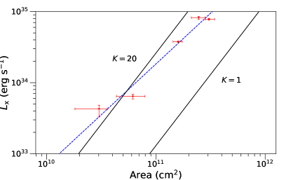
Figure 6.— Trend of the hotspot X-ray luminosity $L_{\rm X}$ in $0.5$–$10\,{\rm keV}$ against the hotspot area $4\pi R_{\rm high}^{2}$ for SGR 0501+4516. The blue dashed line shows the best-fit correlation $L_{\rm X}=1.8\times 10^{34}A_{11}^{1.42}\,{\rm erg}\,{\rm s}^{-1}$ and the black solid lines show the theoretical predicted correlation, $L_{\rm X}=1.3\times 10^{33}KA_{11}^{2}\,{\rm erg}\,{\rm s}^{-1}$, with $K=1$ and $K=20$.

Table 4Blackbody Temperature and Spin-Inferred Magnetic Field Strength of Magnetars and Young High Magnetic Field Rotation-Powered Pulsars as Plotted in Figure 7

Source	$B$ ($10^{14}\,$G)	$kT$ (keV)	Reference
Magnetars (entire surface):
Swift J1822–1606	$0.14$	$0.11\pm 0.01$	See Table 3.3
1E 2259+586	$0.59$	$0.32_{-0.05}^{+0.04}$	See Table 3.3
4U 0142+61	$1.3$	$0.27\pm 0.02$	1
SGR 0501+4516	$1.9$	$0.26_{-0.02}^{+0.01}$	See Table 3.3
XTE J1810–197	$2.1$	$0.167\pm 0.006$	2
CXOU J010043.1–721134	$3.9$	$0.30\pm 0.02$	3
1RXS J170849.0–400910	$4.7$	$0.42\pm 0.02$	4
SGR 0526–66	$5.6$	$0.44\pm 0.02$	5
SGR 1900+14	$7.0$	$0.47\pm 0.02$	6
1E 1841–045	$7.0$	$0.45\pm 0.03$	7
SGR 1806–20	$11.3$	$0.55\pm 0.07$	8
Magnetars (hotspot):
SGR 0418+5729	$0.061$	$0.32\pm 0.05$	9
Swift J1822–1606	$0.14$	$0.29\pm 0.03$	See Table 3.3
1E 2259+586	$0.59$	$0.5_{-0.2}^{+0.1}$	See Table 3.3
CXOU J164710.2–455216	$1.0$	$0.53\pm 0.03$	10
4U 0142+61	$1.3$	$0.50\pm 0.02$	1
SGR 0501+4516	$1.9$	$0.62_{-0.04}^{+0.03}$	See Table 3.3
XTE J1810–197	$2.1$	$0.33\pm 0.02$	2
SGR 1935+2154	$2.2$	$0.47\pm 0.03$	11
1E 1547.0–5408	$2.2$	$0.43\pm 0.05$	12
PSR J1622–4950	$2.7$	$0.5\pm 0.1$	13
CXOU J010043.1–721134	$3.9$	$0.68_{-0.07}^{+0.09}$	3
1E 1048.1–5937	$4.5$	$0.56\pm 0.02$	14
High-$B$ rotation-powered pulsars:
PSR B1509–58	$0.15$	$0.15\pm 0.01$	15
PSR J1119–6127	$0.41$	$0.21\pm 0.04$	16
PSR J1846–0258	$0.49$	$<0.25$	17

Note. —

References. — (1) Gonzalez et al. (2010); (2) Bernardini et al. (2009); (3) Tiengo et al. (2008); (4) Campana et al. (2007); (5) Park et al. (2012); (6) Mereghetti et al. (2006); (7) Kumar & Safi-Harb (2010); (8) Esposito et al. (2007); (9) Rea et al. (2013); (10) An et al. (2013); (11) Israel et al. (2016); (12) Bernardini et al. (2011); (13) Anderson et al. (2012); (14) Tam et al. (2008); (15) Hu et al. (2017); (16) Ng et al. (2012); (17) Livingstone et al. (2011)

4.2. Physical Interpretation of the Hotter Blackbody Component

The best-fit radius of the higher temperature component $R_{\rm high}$ of SGR 0501+4516 had shrunk to $0.49\,{\rm km}$ from 2008 to 2013, indicating that the thermal emission could come from a hotspot on surface. There were several magnetars with blackbody radii that continued to shrink for a few years after their outbursts (Beloborodov & Li, 2016). Beloborodov (2009) suggested that this could be the observational evidence supporting the $j$-bundle model. When a twisted magnetic field is implanted into the closed magnetosphere, the current ($j$-bundle) would flow along the closed magnetic field lines and return back to the stellar surface, heating up the footprints of the $j$-bundle and resulting in hotspots. After an outburst, the footprints are expected to keep shrinking and the hotspot could be observed as a blackbody component with a decreasing radius. This predicts a correlation between the X-ray luminosity and the area of a hotspot as $L_{\rm X}=1.3\times 10^{33}KA_{11}^{2}\,{\rm erg}\,{\rm s}^{-1}$, where $A_{11}$ is the blackbody area in units of $10^{11}\,{\rm cm}^{2}$ and $K$ is a constant depending on the twisting angle of the $j$-bundle, the surface magnetic field strength, and the discharge voltage (Beloborodov, 2009, 2011).
We plot in Figure 6 the hotspot luminosity of SGR 0501+4516 against its area $A=4\pi R_{\rm high}^{2}$. The distance of the source is assumed to be $d=5\,{\rm kpc}$ for calculating the luminosity. Our result broadly agrees with the theory prediction and suggests $K\sim 20$. If we fit the data points with a straight line in the log–log plot in Figure 6, the best-fit correlation is flatter, with $L_{\rm X}=1.8\times 10^{34}A_{11}^{1.42}\,{\rm erg}\,{\rm s}^{-1}$. Similar behavior was also found in several other magnetars during flux relaxation after outbursts (Beloborodov & Li, 2016). The discrepancy could be due to the time variation of the proportionality constant $K$.

4.3. Physical Interpretation of the Cooler Blackbody Component

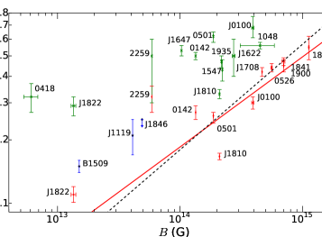
Figure 7.— Blackbody temperature against magnetic field strength of magnetars and three young high-$B$ rotation-powered pulsars, using values listed in Table 4.1. The red and green dots indicate blackbodies from the entire surface and the hotspots, respectively. The blue dots represents the high-$B$ rotation-powered pulsars. The red solid line shows the best-fit correlation $kT\propto B^{0.4}$ using the red data points only. The black dashed line represents the theoretical prediction of $kT\propto B^{0.5}$.

In the two temperature fits, the cooler blackbody always shows a larger radius $R_{\rm low}$ and some values listed in Table 3.3 are compatible with the neutron star radius. We therefore believe that this blackbody component could originate from the entire surface. An additional support is that in our case of SGR 0501+4516, $R_{\rm low}$ has been relatively stable during flux relaxation. Theories suggest that the thermal emission of magnetars could be arise from the decay of the crustal magnetic field (Thompson & Duncan, 1996; Pons et al., 2007). If this is the only energy source, one expects a correlation between the surface temperature $kT$ and the magnetic field strength $B$ (Pons et al., 2007). The conservation of energy could be expressed as

$$-A\Delta R\frac{{\rm d}E_{\rm m}}{{\rm d}t}=A\sigma T^{4},$$ (1)

where $E_{\rm m}$ is the magnetic energy density, $A$ is the emission area, $\Delta R$ is the thickness of the neutron star crust, and $\sigma$ is the Stefan-Boltzmann constant. The magnetic energy density $E_{\rm m}$ could be written as $B^{2}/8\pi$. If the decay of $B$ is in the exponential form, it implies a relation $T\propto\sqrt{B}$. Note that this ignores any age effects that are justified, as magnetars are young objects in general (see Viganò et al., 2013).
To verify the correlation above, we investigated the trend between $kT$ and $B$ for all quiescent magnetars, using the latest results reported in the literature and from our own analysis (see Table 3.3). These values are listed in Table 4.1 and plotted in Figure 7. As we mentioned, some blackbody components correspond to the hotspot and some correspond to the entire surface. We show them separately in the plot as two groups, depending on whether the blackbody radius $R$ is larger or smaller than $3\,{\rm km}$. The plot shows an increasing trend for the entire surface $kT$, with a correlation coefficient $r=0.85$. We fit the log–log plot with a straight line and obtained $kT\propto B^{0.4}$, which is a bit flatter than, but generally comparable with the theoretical prediction of $B^{0.5}$. On the other hand, the temperature of the hotspots shows no such a correlation, which suggests that they could probably be powered by $j$-bundle instead of the decay of the crustal field.

Table 5Quiescent X-Ray Luminosity in $2$–$10\,{\rm keV}$ and Spin-Inferred Magnetic Field Strength of Magnetars and High Magnetic Field Rotation-Powered Pulsars as Plotted in Figure 8

Source	$L_{\rm X}$ ($10^{35}\,{\rm erg}\,{\rm s}^{-1}$)	$B$ $(10^{14}\,{\rm G})$	Distance (kpc)	Reference
Magnetars:
SGR 0418+5729	$1.0_{-0.9}^{+1.1}\times 10^{-5}$	$0.061$	$2.0\pm 0.4$	1
Swift J1822.3–1606	$5_{-4}^{+3}\times 10^{-5}$	$0.14$	$1.6\pm 0.3$	See Table 3.3
1E 2259+586	$0.20_{-0.06}^{+0.04}$	$0.59$	$3.2\pm 0.2$	See Table 3.3
CXOU J164710.2–455216	($4.5\pm 3.8)\times 10^{-3}$	$1.0$	$3.9\pm 0.7$	2
4U 0142+61	$1.05\pm 0.33$	$1.3$	$3.6\pm 0.4$	3
SGR 0501+4516	$3.5_{-1.3}^{+1.0}\times 10^{-2}$	$1.9$	$5.0\pm 1.0$	See Table 3.3
XTE J1810–197	$1.3_{-0.9}^{+0.5}\times 10^{-3}$	$2.1$	$3.1\pm 0.5$	4
1E 1547.0–5408	$1.3_{-0.9}^{+0.5}\times 10^{-2}$	$2.2$	$4.5\pm 0.5$	5
SGR 1627–41	$2.5_{-1.3}^{+2.3}\times 10^{-2}$	$2.2$	$11.0\pm 0.3$	6
PSR J1622–4950	$4.4_{-3.6}^{+7.0}\times 10^{-3}$	$2.7$	$9.0\pm 1.8$	7
CXOU J010043.1–721134	$0.7_{-0.3}^{+1.7}$	$3.9$	$62.4\pm 1.6$	8
1E 1048.1–5937	$0.5\pm 0.3$	$4.5$	$9.0\pm 1.7$	9
1RXS J170849.0–400910	$0.42\pm 0.11$	$4.7$	$3.8\pm 0.5$	10
CXOU J171405.7–381031	$0.33\pm 0.24$	$5.0$	$10.2\pm 3.5$	11
SGR 0526–66	$1.9_{-0.4}^{+0.3}$	$5.6$	$53.6\pm 1.2$	12
SGR 1900+14	$0.7\pm 0.3$	$7.0$	$12.5\pm 1.7$	13
1E 1841–045	$1.8_{-1.0}^{+0.7}$	$7.0$	$8.5_{-1.0}^{+1.3}$	14
SGR 1806–20	$1.6_{-0.7}^{+0.8}$	$11.3$	$8.7_{-1.5}^{+1.8}$	15
High-$B$ rotation-powered pulsars:
PSR B1509–58	$0.96\pm 0.05$	$0.15$	$5.2\pm 1.4$	16
PSR J1119–6127	$2.5_{-1.3}^{+3.2}\times 10^{-3}$	$0.41$	$8.4\pm 0.4$	17
PSR J1846–0258	$0.19_{-0.03}^{+0.04}$	$0.49$	$6.0_{-0.9}^{+1.5}$	18

Note. —

References. — (1) Rea et al. (2013); (2) An et al. (2013); (3) Rea et al. (2007); (4) Bernardini et al. (2009); (5) Gelfand & Gaensler (2007); (6) Esposito et al. (2008); (7) Anderson et al. (2012); (8) Tiengo et al. (2008); (9) Tam et al. (2008); (10) Rea et al. (2007); (11) Sato et al. (2010); (12) Park et al. (2012); (13) Nakagawa et al. (2009); (14) Kumar & Safi-Harb (2010); (15) Esposito et al. (2007); (16) Hu et al. (2017); (17) Ng et al. (2012); (18) Livingstone et al. (2011)

There is recent evidence showing that both young high magnetic field rotation-powered pulsars and magnetars share similar properties, making the division between these two classes blurred (see Gavriil et al., 2008; Ng & Kaspi, 2011; Göğüş et al., 2016). This motivates us to include the three young sources with age of $\sim 10^{3}\,{\rm years}\,$, PSRs B1509–58, J1119–6127, and J1846–0258, in Table 4.1 and Figure 7 for comparison. The thermal emission of PSRs B1509–58 and J1119–6127 has blackbody radii $R=10^{+39}_{-5}\,{\rm km}$ and $3^{+4}_{-1}\,{\rm km}$, respectively, suggesting that they could be originated from the entire surface (or large area; Ng et al. 2012; Hu et al. 2017). However, for PSR B1509–58, the blackbody radius was not very well constrained due to strong non-thermal emission. On the other hand, there is no thermal emission found in PSR J1846–0258 in quiescence, with an upper limit of $0.25\,{\rm keV}$ (Livingstone et al., 2011). From the plot, it is interesting to note that all high-$B$ rotation-powered pulsars seem to follow the same $kT$–$B$ trend as magnetars. Our results suggest that the energy source, i.e. $B$-field decay, could power the entire surface thermal emission of magnetars and high-$B$ rotation-powered pulsars.
While $kT$ and $B$ appear to show a correlation that is broadly consistent with the theory, there remain some unsolved problems in this picture. The temperature of the cooler blackbody component is typically higher in outburst, then decays to a constant value a few years after. Hence, the outburst could partly contributed to the thermal emission (see Figure 4 and also Bernardini et al. 2009 and Gonzalez et al. 2010). Also, we note that some radii of the cooler blackbody are smaller than that of a neutron star. It could indicate that the emission regions are smaller than the entire surface or that the temperature distribution is inhomogeneous. It is unclear if the Equation 1 needs to be modified in this case.

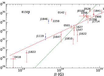
Figure 8.— X-ray luminosity $L_{\rm X}$ in $2$–$10\,{\rm keV}$ against magnetic field strength $B$, using values listed in Table 4.3. The red dots indicate magnetars in quiescence, and the blue dots indicate high-$B$ rotation-powered pulsars. The red and the green dashed lines show the theoretical predictions of $L_{\rm X}\propto B^{2}$ and $\propto B^{4.4}$, respectively.

4.4. Correlation Between X-Ray Luminosity and Magnetic Field

We revisit the correlation between the quiescent X-ray luminosity, $L_{\rm X}$, and the magnetic field, $B$, of magnetars as reported by An et al. (2012), using updated measurements listed in Table 4.3. The results are plotted in Figure 8. We compared the trend with two theoretical predictions of $L_{\rm X}\propto B^{2}$ deduced from the Equation 1 (Pons et al., 2007) and $L_{\rm X}\propto B^{4.4}$ based on the ambipolar diffusion model with neutrino cooling (Thompson & Duncan, 1996). The plot shows a general trend but with large scatter, particularly for magnetars with $B\sim 10^{14}\,{\rm G}$. Our updated plot prefers $B^{2}$, providing some support to the simple magnetic field decay model. Note that our result contradicts that reported by An et al. (2012). The main discrepancy is due to the updated measurements from two low-field magnetars, SGR 0418+5729 and Swift J1822.3–1606. If we fit the log–log plot with a straight line, we obtain a slightly flatter correlation of $L_{\rm X}\propto B^{1.7}$. From the plot, 1E 2259+586 and 4U 0142+61 are far more luminous than other magnetars with similar $B$. Excluding these two outliers gives $L_{\rm X}\propto B^{2.8}$, which again prefers $B^{2}$ to $B^{4.4}$.
Similar to the $kT$–$B$ plot, we also include three young high magnetic field rotation-powered pulsars in Figure 8. We found that only PSR J1119–6127 follows the general trend of magnetars, while the other two, PSRs B1509–58 and J1846–0258, have luminosities a few orders of magnitude higher. We believe that their X-ray emission is dominated by non-thermal radiation powered by spin-down, which could be a main difference between magnetars and high-$B$ rotation-powered pulsars. Although the correlation appears to support to the theoretical prediction, there are too few magnetar examples with $B<10^{14}\,{\rm G}$. Increasing the sample in this magnetic field range in future studies can better confirm the theory.

5. CONCLUSION

We performed spectral and timing analyses of SGR 0501+4516 using new and archival X-ray observations taken with Chandra, XMM-Newton, and Suzaku. We show that the source has returned to quiescence in 2013, five years after the outburst. Our timing results found a spin period of $\sim 5.762\,{\rm s}$ with stable pulse profiles in 2012 and 2013. The Chandra images show no detectable proper motion, with an upper limit of $0\farcs 32\,{\rm yr}^{-1}$, rejecting the idea that SGR 0501+4516 was born in SNR G160.9+2.6. We found that the soft X-ray spectrum is best described by a double blackbody plus power-law (2BB+PL) model. The quiescent spectrum has temperatures of $0.26\,{\rm keV}$ (with $R=3.7\,{\rm km}$) and $0.62\,{\rm keV}$ (with $R=0.49\,{\rm km}$). We found a correlation between the X-ray luminosity and the area of the evolving hotter blackbody component, which agrees with the prediction of the $j$-bundle model.
We further applied the two-temperature spectral model to other magnetars in quiescence and found that it provides a good fit to most sources with low column density, suggesting that this could be a common feature. We investigated the correlation between the blackbody temperature $kT$ and the spin-inferred magnetic field $B$ of all magnetars in quiescence. For blackbodies with large areas comparable to the entire stellar surface, the correlation generally agrees with the prediction from the simple magnetic field decay model. We found that this simple scenario can also explain the trend between the quiescent X-ray luminosity and magnetic field strength of magnetars.

References

- An et al. (2013) An, H., Kaspi, V. M., Archibald, R., & Cumming, A. 2013, ApJ, 763, 82
- An et al. (2012) An, H., Kaspi, V. M., Tomsick, J. A., et al. 2012, ApJ, 757, 68
- Anderson et al. (2012) Anderson, G. E., Gaensler, B. M., Slane, P. O., et al. 2012, ApJ, 751, 53
- Barthelmy et al. (2008) Barthelmy, S. D., Baumgartner, W. H., Beardmore, A. P., et al. 2008, The Astronomer’s Telegram, 1676, 1
- Beloborodov (2009) Beloborodov, A. M. 2009, ApJ, 703, 1044
- Beloborodov (2011) Beloborodov, A. M. 2011, Astrophysics and Space Science Proceedings, 21, 299
- Beloborodov & Li (2016) Beloborodov, A. M., & Li, X. 2016, ApJ, 833, 261
- Bernardini et al. (2009) Bernardini, F., Israel, G. L., Dall’Osso, S., et al. 2009, A&A, 498, 195
- Bernardini et al. (2011) Bernardini, F., Israel, G. L., Stella, L., et al. 2011, A&A, 529, A19
- Camero et al. (2014) Camero, A., Papitto, A., Rea, N., et al. 2014, MNRAS, 438, 3291
- Campana et al. (2007) Campana, S., Rea, N., Israel, G. L., Turolla, R., & Zane, S. 2007, A&A, 463, 1047
- Enoto et al. (2010) Enoto, T., Rea, N., Nakagawa, Y. E., et al. 2010, ApJ, 715, 665
- Enoto et al. (2017) Enoto, T., Shibata, S., Kitaguchi, T., et al. 2017, ApJS, 231, 8
- Esposito et al. (2007) Esposito, P., Mereghetti, S., Tiengo, A., et al. 2007, A&A, 476, 321
- Esposito et al. (2008) Esposito, P., Israel, G. L., Zane, S., et al. 2008, MNRAS, 390, L34
- Freeman et al. (2001) Freeman, P., Doe, S., & Siemiginowska, A. 2001, Proc. SPIE, 4477, 76
- Fruscione et al. (2006) Fruscione, A., McDowell, J. C., Allen, G. E., et al. 2006, Proc. SPIE, 6270, 62701V
- Gaensler & Chatterjee (2008) Gaensler, B. M., & Chatterjee, S. 2008, GRB Coordinates Network, 8149, 1
- Gavriil et al. (2008) Gavriil, F. P., Gonzalez, M. E., Gotthelf, E. V., et al. 2008, Science, 319, 1802
- Gelfand & Gaensler (2007) Gelfand, J. D., & Gaensler, B. M. 2007, ApJ, 667, 1111
- Gonzalez et al. (2010) Gonzalez, M. E., Dib, R., Kaspi, V. M., et al. 2010, ApJ, 716, 1345
- Göğüş et al. (2016) Göğüş, E., Lin, L., Kaneko, Y., et al. 2016, ApJ, 829, L25
- Göǧüş et al. (2010) Göǧüş, E., Woods, P. M., Kouveliotou, C., et al. 2010, ApJ, 722, 899
- Hu et al. (2017) Hu, C.-P., Ng, C.-Y., Takata, J., Shannon, R. M., & Johnston, S. 2017, ApJ, 838, 156
- Israel et al. (2016) Israel, G. L., Esposito, P., Rea, N., et al. 2016, MNRAS, 457, 3448
- Kaspi & Beloborodov (2017) Kaspi, V. M., & Beloborodov, A. M. 2017, ARA&A, 55, 261
- Kumar & Safi-Harb (2010) Kumar, H. S., & Safi-Harb, S. 2010, ApJ, 725, L191
- Leahy (1987) Leahy, D. A. 1987, A&A, 180, 275
- Leahy & Tian (2007) Leahy, D. A., & Tian, W. W. 2007, A&A, 461, 1013
- Livingstone et al. (2011) Livingstone, M. A., Ng, C.-Y., Kaspi, V. M., Gavriil, F. P., & Gotthelf, E. V. 2011, ApJ, 730, 66
- Lyubarsky et al. (2002) Lyubarsky, Y., Eichler, D., & Thompson, C. 2002, ApJ, 580, L69
- Mereghetti et al. (2006) Mereghetti, S., Esposito, P., Tiengo, A., et al. 2006, ApJ, 653, 1423
- Nakagawa et al. (2009) Nakagawa, Y. E., Mihara, T., Yoshida, A., et al. 2009, PASJ, 61, S387
- Ng & Kaspi (2011) Ng, C.-Y., & Kaspi, V. M. 2011, AIP Conf. Proc. 1379, Astrophysics of Neutron Stars 2010: A Conference in Honor of Ali Alpar, M., ed. Göğüş, E. and Belloni, T. and Ertan, Ü. (Melville, NY: AIP), 60
- Ng et al. (2012) Ng, C.-Y., Kaspi, V. M., Ho, W. C. G., et al. 2012, ApJ, 761, 65
- Olausen & Kaspi (2014) Olausen, S. A., & Kaspi, V. M. 2014, ApJS, 212, 6
- Parfrey et al. (2012) Parfrey, K., Beloborodov, A. M., & Hui, L. 2012, ApJ, 754, L12
- Parfrey et al. (2013) Parfrey, K., Beloborodov, A. M., & Hui, L. 2013, ApJ, 774, 92
- Park et al. (2012) Park, S., Hughes, J. P., Slane, P. O., et al. 2012, ApJ, 748, 117
- Pons et al. (2007) Pons, J. A., Link, B., Miralles, J. A., & Geppert, U. 2007, Physical Review Letters, 98, 071101
- Rea et al. (2008) Rea, N., Zane, S., Turolla, R., Lyutikov, M., & Götz, D. 2008, ApJ, 686, 1245
- Rea et al. (2007) Rea, N., Nichelli, E., Israel, G. L., et al. 2007, MNRAS, 381, 293
- Rea et al. (2007) Rea, N., Israel, G. L., Oosterbroek, T., et al. 2007, Ap&SS, 308, 505
- Rea et al. (2009) Rea, N., Israel, G. L., Turolla, R., et al. 2009, MNRAS, 396, 2419
- Rea et al. (2013) Rea, N., Israel, G. L., Pons, J. A., et al. 2013, ApJ, 770, 65
- Sato et al. (2010) Sato, T., Bamba, A., Nakamura, R., & Ishida, M. 2010, PASJ, 62, L33
- Tam et al. (2008) Tam, C. R., Gavriil, F. P., Dib, R., et al. 2008, ApJ, 677, 503-514
- Thompson & Duncan (1995) Thompson, C., & Duncan, R. C. 1995, MNRAS, 275, 255
- Thompson & Duncan (1996) Thompson, C., & Duncan, R. C. 1996, ApJ, 473, 322
- Thompson & Duncan (2001) Thompson, C., & Duncan, R. C. 2001, ApJ, 561, 980
- Thompson et al. (2000) Thompson, C., Duncan, R. C., Woods, P. M., et al. 2000, ApJ, 543, 340
- Thompson et al. (2002) Thompson, C., Lyutikov, M., & Kulkarni, S. R. 2002, ApJ, 574, 332
- Tiengo et al. (2008) Tiengo, A., Esposito, P., & Mereghetti, S. 2008, ApJ, 680, L133
- van der Horst et al. (2010) van der Horst, A. J., Connaughton, V., Kouveliotou, C., et al. 2010, ApJ, 711, L1
- Viganò et al. (2013) Viganò, D., Rea, N., Pons, J. A., et al. 2013, MNRAS, 434, 123
- Weng & Göğüş (2015) Weng, S.-S., & Göğüş, E. 2015, ApJ, 815, 15
- Wilms et al. (2000) Wilms, J., Allen, A., & McCray, R. 2000, ApJ, 542, 914
- Woods et al. (2008) Woods, P. M., Gogus, E., & Kouveliotou, C. 2008, The Astronomer’s Telegram, 1691, 1
- Zhu et al. (2008) Zhu, W., Kaspi, V. M., Dib, R., et al. 2008, ApJ, 686, 520