A discrete event traffic model explaining the traffic phases of the train dynamics in a metro line system with a junction

Abstract

This paper presents a mathematical model for the train dynamics in a mass-transit metro line system with one symmetrically operated junction. We distinguish three parts: a central part and two branches. The tracks are spatially discretized into segments (or blocks) and the train dynamics are described by a discrete event system where the variables are the $k^{th}$ departure times from each segment. The train dynamics are based on two main constraints: a travel time constraint modeling theoretic run and dwell times, and a safe separation constraint modeling the signaling system in case where the traffic gets very dense. The Max-plus algebra model allows to analytically derive the asymptotic average train frequency as a function of many parameters, including train travel times, minimum safety intervals, the total number of trains on the line and the number of trains on each branch. This derivation permits to understand the physics of traffic. In a further step, the results will be used for traffic control.

Keywords. Physics of traffic, Discrete event systems, Max-plus algebra, Traffic control, Transportation networks.

I Introduction and Literature review

Mass-transit metro lines are generally driven on their capacity limit to satisfy the high demand. Among the different network topologies for metro lines, those with a junction are much more sensible to perturbations than simple ring or linear lines. RATP, the operator of the French capital’s metro system, runs several metro and rapid transit lines with convergences.

The here presented model for a metro line with a symmetrically operated junction describes the dynamics of the system with static run and dwell times which respect lower bounds. The model permits a comprehension of the physics of traffic for this case, by an analytic derivation of the train frequency in function of the parameters of the line (number of moving trains, safe separation times, etc).

We base this work on the traffic models presented in [4, 5, 6], where the physics of traffic in a metro line system without junction are entirely described. It is a discrete event modeling approach, where we use train departure times as the main modeling variables. Two cases have been studied in [4, 5, 6].

The first case assumes that the train dwell times on platforms respect given lower bounds. It has been shown that in this case, the train dynamics can be written linearly in the Max-plus algebra. This formulation permitted to show that the traffic dynamic admits a unique asymptotic regime. Moreover, the asymptotic average train time-headway is derived analytically in function of the number of trains moving on the line and other parameters like train speed and safe separation time.

The second case proposes a real-time control of the train dwell times depending on passenger demand which will be subject to further works on the here presented traffic model.

The Max-plus theory being used here, has further been subject to recent research by Goverde [7] to analyze railway timetable stability. Black-box optimization algorithms for real-time railway rescheduling have been treated in research for a long time. Cacchiani et al. [2] give a state of the art review of these recovery models and algorithms. Schanzenbächer et al. [9] have applied such an optimal holding control for dwell optimization to a mass transit railway line in the Paris area. Li et al. [8] present an optimal control approach for train regulation and passenger flow control on high-frequency metro lines without a junction.

After a review on Max-plus algebra, we introduce the model of our plant and derive the traffic phases of the system.

II Review on linear Max-plus algebra systems

Max-plus algebra [1] is the idempotent commutative semi-ring $(\mathbb{R}\cup\{-\infty\},\oplus,\otimes)$, where the operations $\oplus$ and $\otimes$ are defined by: $a\oplus b=\max\{a,b\}$ and $a\otimes b=a+b$. The zero element is $(-\infty)$ denoted by $\varepsilon$ and the unity element is $0$ denoted by $e$. On the set of square matrices, if $A$ and $B$ are two Max-plus matrices of size $n\times n$, the addition $\oplus$ and the product $\otimes$ are defined by: $(A\oplus B)_{ij}:=A_{ij}\oplus B_{ij},\forall i,j$, and $(AB)_{i,j}=(A\otimes B)_{ij}:=\bigoplus_{k}[A_{ik}\otimes B_{kj}]$. The zero and the unity matrices are also denoted by $\varepsilon$ and $e$ respectively.

Let us now consider the dynamics of a homogeneous $p$-order Max-plus system with a family of Max-plus matrices $A_{l}$

$$x(k)=\bigoplus_{l=0}^{p}A_{l}\otimes x(k-l).$$ (1)

We define $\gamma$ as the backshift operator applied on the sequences on $\mathbb{Z}$: $\gamma^{l}x(k)=x(k-l),\forall l\in\mathbb{N}$. Then (1) can be written

$$x(k)=\bigoplus_{l=0}^{p}\gamma^{l}A_{l}x(k)=A(\gamma)x(k),$$ (2)

where $A(\gamma)=\bigoplus_{l=0}^{p}\gamma^{l}A_{l}$ is a polynomial matrix in the backshift operator $\gamma$; see [1, 7] for more details.

$\mu\in\mathbb{R}_{\max}\setminus\{\varepsilon\}$ is said to be a generalized eigenvalue [3] of $A(\gamma)$, with associated generalized eigenvector $v\in\mathbb{R}_{\max}^{n}\setminus\{\varepsilon\}$, if

$$A(\mu^{-1})\otimes v=v,$$ (3)

where $A(\mu^{-1})$ is the matrix obtained by evaluating the polynomial matrix $A(\gamma)$ at $\mu^{-1}$.

A directed graph denoted $\mathcal{G}(A(\gamma))$ can be associated to a dynamic system of type (2). For every $l,0\leq l\leq p$, an arc $(i,j,l)$ is associated to each non-null ($\neq\varepsilon$) element $(i,j)$ of Max-plus matrix $A_{l}$. A weight $W(i,j,l)$ and a duration $D(i,j,l)$ are associated to each arc $(i,j,l)$ in the graph, with $W(i,j,l)=(A_{l})_{ij}\neq\varepsilon$ and $D(i,j,l)=l$. Similarly, a weight, resp. duration of a cycle (a directed cycle) in the graph is the standard sum of the weights, resp. durations of all the arcs of the cycle. Finally, the cycle mean of a cycle $c$ with a weight $W(c)$ and a duration $D(c)$ is $W(c)/D(c)$. A polynomial matrix $A(\gamma)$ is said to be irreducible, if $\mathcal{G}(A(\gamma))$ is strongly connected.

We recall here a result that we will use in the next sections.

Theorem 1

[1, Theorem 3.28] [7, Theorem 1] Let $A(\gamma)=\oplus_{l=0}^{p}A_{l}\gamma^{l}$ be an irreducible polynomial matrix with acyclic sub-graph $\mathcal{G}(A_{0})$. Then $A(\gamma)$ has a unique generalized eigenvalue $\mu>\varepsilon$ and finite eigenvectors $v>\varepsilon$ such that $A(\mu^{-1})\otimes v=v$, and $\mu$ is equal to the maximum cycle mean of $\mathcal{G}(A(\gamma))$, given as follows: $\mu=\max_{c\in\mathcal{C}}W(c)/D(c)$, where $\mathcal{C}$ is the set of all elementary cycles in $\mathcal{G}(A(\gamma))$. Moreover, the dynamic system $x(k)=A(\gamma)x(k)$ admits an asymptotic average growth vector (also called cycle time vector here) $\chi$ whose components are all equal to $\mu$.

III Train dynamics in a metro line system with a junction

We extend the approach developed in [4, 5, 6] by modeling a metro line with a junction. Let us consider a metro line with one junction as shown in Figure 1 below. As in [4, 5, 6], the line is discretized in a number of segments (or sections, or blocks). We call node here the point separating two consecutive segments on the line. Segments and nodes are indexed as in Figure 1.

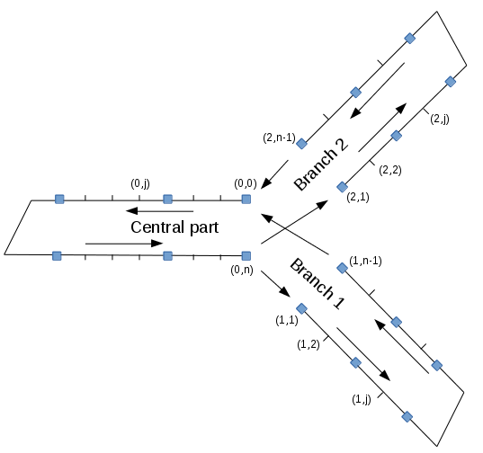
Figure 1: Schema of a metro line with one junction and the corresponding notation.

Let us consider the following notations:

$u$	$\in\mathcal{U}=\{0,1,2\}$ indexes the central part if
	$u=0$, branch 1 if $u=1$, branch 2 if $u=2$.
$n_{u}$	the number of segments on part $u$ of the line.
$m_{u}$	the number of trains being on the part $u$ of the
	line, at time zero.
$b_{(u,j)}$	$\in\{0,1\}$. It is $O$ (resp. $1$) if there is no
	train (resp. one train) at segment $j$ of part $u$.
$\bar{b}_{(u,j)}$	$=1-b_{(u,j)}$.
$d^{k}_{(u,j)}$	the $k^{\text{th}}$ departure time from node $j$, on part $u$
	of the line. Notice that $k$ does not index trains,
	but count the number of train departures.
$a^{k}_{(u,j)}$	the $k^{\text{th}}$ arrival time to node $j$, on part $u$
	of the line.
$r{(u,j)}$	the average running time of trains on segment $j$
	(between nodes $j-1$ and $j$) of part $u$.
$w^{k}_{(u,j)}$	$=d^{k}_{(u,j)}-a^{k}_{(u,j)}$ the $k^{\text{th}}$ dwell time on node $j$
	on part $u$ of the line.
$t^{k}_{(u,j)}$	$=r_{(u,j)}+w^{k}_{(u,j)}$ the $k^{\text{th}}$ travel time from node
	$j-1$ to node $j$ on part $u$ of the line.
$g^{k}_{(u,j)}$	$=a^{k}_{(u,j)}-d^{k-1}_{(u,j)}$ the $k^{\text{th}}$ safe separation time
	(or close-in time) at node $j$ on part $u$.

$h^{k}_{(u,j)}$	$=d^{k}_{(u,j)}-d^{k-1}_{(u,j)}=g^{k}_{(u,j)}+w^{k}_{(u,j)}$ the $k^{\text{th}}$
	departure time-headway at node $j$ on part $u$.
$s^{k}_{(u,j)}$	$=g^{k+b_{(u,j)}}_{(u,j)}-r_{(u,j)}$.

We also use underline notations to note the minimum bounds of the corresponding variables respectively. Then $\underline{r}_{(u,j)},\underline{t}_{(u,j)},\underline{w}_{(u,j)},\underline{g}_{(u,j)},\underline{h}_{(u,j)}$ and $\underline{s}_{(u,j)}$ denote respectively minimum running, travel, dwell, safe separation, headway and $s$ times.

The (asymptotic) averages on $j$ and on $k$ of those variables are denoted without any subscript or superscript. Then $r,t,w,g,h$ and $s$ denote the average running, travel, dwell, safe separation, headway and $s$ times, respectively.

It is easy to check the following relationships:

$$g_{u}=r_{u}+s_{u},$$ (4)

$$t_{u}=r_{u}+w_{u},$$ (5)

$$h_{u}=g_{u}+w_{u}=r_{u}+w_{u}+s_{u}=t_{u}+s_{u}.$$ (6)

We give below the train dynamics in the metro line system. We distinguish the dynamics on the tracks out of the junction, with the ones on the divergence and on the merge.

III-A Train dynamics out of the junction

We model the train dynamics here as in [4, 5, 6]. Two main constraints are considered to describe the train dynamics out of the junction.

• The $k^{\text{th}}$ train departure from node $j$ (of any part of the line) corresponds to the $k^{\text{th}}$ train departure from node $j-1$ in case where there was no train on segment $j$ at time zero; and it corresponds to the $(k-1)^{\text{th}}$ train departure from node $j-1$ in case where there was a train on segment $j$ at time zero. Between two consecutive departures, a minimum time of $\underline{t}_{(u,j)}$ is respected. We write

  $$d^{k}_{(u,j)}\geq d^{k-b_{(u,j)}}_{(u,j-1)}+\underline{t}_{(u,j)},\;\forall k\geq 0,u\in\mathcal{U},j\neq n_{u}.$$ (7)

• The $k^{\text{th}}$ train departure from node $j$ must be preceded by the $(k-1)^{\text{th}}$ train departure from node $j+1$ plus a minimum time $\underline{s}^{k}_{(u,j)}$ in case where there was no train on segment $j+1$ at time zero; and it must be preceded by the $k^{\text{th}}$ train departure from node $j+1$ plus a minimum time $\underline{s}^{k}_{(u,j)}$ in case where there was a train on segment $j+1$ at time zero. We write

  $$d^{k}_{(u,j)}\geq d^{k-\bar{b}_{(u,j+1)}}_{(u,j+1)}+\underline{s}_{(u,j+1)},\;\forall k\geq 0,u\in\mathcal{U},j\neq n_{u}.$$ (8)

We assume here that a train departs from node $j$ out of the junction, as soon as the two constraints (7) and (8) are satisfied. We get

$$d^{k}_{(u,j)}=\max\left\{d^{k-b_{(u,j)}}_{(u,j-1)}+\underline{t}_{(u,j)},d^{k-\bar{b}_{(u,j+1)}}_{(u,j+1)}+\underline{s}_{(u,j+1)}\right\}.$$ (9)

This assumption holds for all couples of constraints we will propose below. This will permit us to write the whole train dynamics as a homogeneous Max-plus system.

III-B Train dynamics on the divergence

We assume here that trains leaving the central part of the line and going to the branches respect the following rule. Odd departures go to branch 1 while even departures go to branch 2. We then have the following constraints.

The $k^{\text{th}}$ departures from the central part:

$$d^{k}_{(0,n)}\geq d^{k-b_{(0,n)}}_{(0,n-1)}+\underline{t}_{(0,n)},\;\forall k\geq 0,\\$$ (10)

$$d^{k}_{(0,n)}\geq\begin{cases}d^{(k+1)/2-\bar{b}_{(1,1)}}_{(1,1)}+\underline{s}_{(1,1)}&\text{if }k\text{ is odd}\\ ~{}~{}\\ d^{k/2-\bar{b}_{(2,1)}}_{(2,1)}+\underline{s}_{(2,1)}&\text{if }k\text{ is even}\\ \end{cases}$$ (11)

The $k^{\text{th}}$ departures from the entry of branch 1:

$$d^{k}_{(1,1)}\geq d^{(2k-1)-b_{(1,1)}}_{(0,n)}+\underline{t}_{(1,1)},\;\forall k\geq 0,$$ (12)

$$d^{k}_{(1,1)}\geq d^{k-\bar{b}_{(1,2)}}_{(1,2)}+\underline{s}_{(1,2)},\;\forall k\geq 0.$$ (13)

The $k^{\text{th}}$ departures from the entry of branch 2:

$$d^{k}_{(2,1)}\geq d^{2k-b_{(2,1)}}_{(0,n)}+\underline{t}_{(2,1)},\;\forall k\geq 0,$$ (14)

$$d^{k}_{(2,1)}\geq d^{k-\bar{b}_{(2,2)}}_{(2,2)}+\underline{s}_{(2,2)},\;\forall k\geq 0.$$ (15)

III-C Train dynamics on the merge

We assume here that trains entering to the central part of the line from the two branches respect the following rule. Odd departures at node $(0,0)$ towards the central part correspond to trains coming from branch 1 while even ones correspond to trains coming from branch 2.

The $k^{\text{th}}$ departures from the central part:

$$d^{k}_{(0,0)}\geq\begin{cases}d^{(k+1)/2-b_{(1,n)}}_{(1,n-1)}+\underline{t}_{(1,n)}&\text{if }k\text{ is odd}\\ ~{}~{}\\ d^{k/2-b_{(2,n)}}_{(2,n-1)}+\underline{t}_{(2,n)}&\text{if }k\text{ is even}\\ \end{cases}$$ (16)

$$d^{k}_{(0,0)}\geq d^{k-\bar{b}_{(0,1)}}_{(0,1)}+\underline{s}_{(0,1)},\;\forall k\geq 0,\\$$ (17)

The $k^{\text{th}}$ departures from the entry of branch 1:

$$d^{k}_{(1,n-1)}\geq d^{k-b_{(1,n-1)}}_{(1,n-2)}+\underline{t}_{(1,n-1)},\;\forall k\geq 0,$$ (18)

$$d^{k}_{(1,n-1)}\geq d^{(2k-1)-\bar{b}_{(1,n)}}_{(0,0)}+\underline{s}_{(1,n)},\;\forall k\geq 0.$$ (19)

The $k^{\text{th}}$ departures from the entry of branch 2:

$$d^{k}_{(2,n-1)}\geq d^{k-b_{(2,n-1)}}_{(2,n-2)}+\underline{t}_{(2,n-1)},\;\forall k\geq 0,$$ (20)

$$d^{k}_{(2,n-1)}\geq d^{2k-\bar{b}_{(2,n)}}_{(0,0)}+\underline{s}_{(2,n)},\;\forall k\geq 0.$$ (21)

IV Max-plus algebra modeling

In order to avoid multiplicative backshifts between the departures on the central part and the ones on the branches, we introduce a change of variables in this section. Let us look at the dynamic given by (12). $d^{k}_{(1,1)}$ is given as a function of $d^{2k-1-b_{(1,1)}}_{(0,n)}$. We see clearly that the two sequences do not have the same growth speed. Indeed, the growth rate of $d_{(0,n)}$ is about double the one of $d_{(1,1)}$. This is due to the fact that every second train moving on the central part of the line goes to branch 1.

In order to have all the sequences of the train dynamics growing with the same speed, and then be able to write the dynamics as a homogeneous Max-plus system, we introduce the following change of variables:

$$\delta^{k}_{(0,j)}=d^{k}_{(0,j)},\forall k\geq 0,\forall j$$ (22)

$$\delta^{2k}_{(1,j)}=d^{k}_{(1,j)},\forall k\geq 0,\forall j$$ (23)

$$\delta^{2k}_{(2,j)}=d^{k}_{(2,j)},\forall k\geq 0,\forall j.$$ (24)

In the following, we rewrite all the train dynamics with the change of variables defined above.

IV-A New train dynamics out of the junction

The train dynamics out of the junction are written as follows.

On the central part, it is sufficient to replace $d$ with $\delta$:

$$\delta^{k}_{(0,j)}\geq\delta^{k-b_{(0,j)}}_{(0,j-1)}+\underline{t}_{(0,j)},\;\forall k\geq 0,j\neq n_{u},$$ (25)

$$\delta^{k}_{(0,j)}\geq\delta^{k-\bar{b}_{(0,j+1)}}_{(0,j+1)}+\underline{s}_{(0,j+1)},\;\forall k\geq 0,j\neq n_{u}.$$ (26)

For the dynamics on the branches, we get

$$\delta^{k}_{(u,j)}\geq\delta^{k-2b_{(u,j)}}_{(u,j-1)}+\underline{t}_{(u,j)},\;\forall k\geq 0,u\in\{1,2\},j\neq n_{u},$$ (27)

$$\delta^{k}_{(u,j)}\geq\delta^{k-2\bar{b}_{(u,j+1)}}_{(u,j+1)}+\underline{s}_{(u,j+1)},\;\forall k\geq 0,u\in\{1,2\},j\neq n_{u}.$$ (28)

IV-B New train dynamics on the divergence

The dynamics on the divergence are rewritten as follows.

The $k^{\text{th}}$ departures from the central part:

$$\delta^{k}_{(0,n)}\geq\delta^{k-b_{(0,n)}}_{(0,n-1)}+\underline{t}_{(0,n)},\;\forall k\geq 0,\\$$ (29)

$$\delta^{k}_{(0,n)}\geq\begin{cases}\delta^{(k+1)-2\bar{b}_{(1,1)}}_{(1,1)}+\underline{s}_{(1,1)}&\text{for }k\text{ is odd}\\ ~{}~{}\\ \delta^{k-2\bar{b}_{(2,1)}}_{(2,1)}+\underline{s}_{(2,1)}&\text{for }k\text{ is even}\\ \end{cases}$$ (30)

The $k^{\text{th}}$ departures from the entry of branch 1:

$$\delta^{k}_{(1,1)}\geq\delta^{(k-1)-2b_{(1,1)}}_{(0,n)}+\underline{t}_{(1,1)},\;\forall k\geq 0,$$ (31)

$$\delta^{k}_{(1,1)}\geq\delta^{k-2\bar{b}_{(1,2)}}_{(1,2)}+\underline{s}_{(1,2)},\;\forall k\geq 0.$$ (32)

The $k^{\text{th}}$ departures from the entry of branch 2:

$$\delta^{k}_{(2,1)}\geq\delta^{k-2b_{(2,1)}}_{(0,n)}+\underline{t}_{(2,1)},\;\forall k\geq 0,$$ (33)

$$\delta^{k}_{(2,1)}\geq\delta^{k-2\bar{b}_{(2,2)}}_{(2,2)}+\underline{s}_{(2,2)},\;\forall k\geq 0.$$ (34)

IV-C New train dynamics on the merge

The dynamics on the merge are rewritten as follows.

The $k^{\text{th}}$ departures from the central part:

$$\delta^{k}_{(0,0)}\geq\begin{cases}\delta^{(k+1)-2b_{(1,n)}}_{(1,n-1)}+\underline{t}_{(1,n)}&\text{for }k\text{ is odd}\\ ~{}~{}\\ \delta^{k-2b_{(2,n)}}_{(2,n-1)}+\underline{t}_{(2,n)}&\text{for }k\text{ is even}\\ \end{cases}$$ (35)

$$\delta^{k}_{(0,0)}\geq\delta^{k-2\bar{b}_{(0,1)}}_{(0,1)}+\underline{s}_{(0,1)},\;\forall k\geq 0,\\$$ (36)

The $k^{\text{th}}$ departures from the entry of branch 1:

$$\delta^{k}_{(1,n-1)}\geq\delta^{k-2b_{(1,n-1)}}_{(1,n-2)}+\underline{t}_{(1,n-1)},\;\forall k\geq 0,$$ (37)

$$\delta^{k}_{(1,n-1)}\geq\delta^{(k-1)-2\bar{b}_{(1,n)}}_{(0,0)}+\underline{s}_{(1,n)},\;\forall k\geq 0.$$ (38)

The $k^{\text{th}}$ departures from the entry of branch 2:

$$\delta^{k}_{(2,n-1)}\geq\delta^{k-2b_{(2,n-1)}}_{(2,n-2)}+\underline{t}_{(2,n-1)},\;\forall k\geq 0,$$ (39)

$$\delta^{k}_{(2,n-1)}\geq\delta^{k-2\bar{b}_{(2,n)}}_{(0,0)}+\underline{s}_{(2,n)},\;\forall k\geq 0.$$ (40)

IV-D Train dynamics in Max-plus algebra

Let us now show how all the train dynamics given above are written in Max-plus algebra. First, as already mentioned above, we assume for every couple of constraints written on the departure from a given node, that the departure in question is realized as soon as the two associated constraints are satisfied. For example, with this assumption, constraints (25) and (26) give

$$\delta^{k}_{(0,j)}=\max\left\{\delta^{k-b_{(0,j)}}_{(0,j-1)}+\underline{t}_{(0,j)},\delta^{k-\bar{b}_{(0,j+1)}}_{(0,j+1)}+\underline{s}_{(0,j+1)}\right\}.$$ (41)

which is written in Max-plus algebra as follows:

$$\delta_{(0,j)}=\gamma^{b_{(0,j)}}\underline{t}_{(0,j)}\delta_{(0,j-1)}\oplus\gamma^{\bar{b}_{(0,j+1)}}\underline{s}_{(0,j+1)}\delta_{(0,j+1)}.$$ (42)

We can easily check that all the couples of constraints of the whole dynamics can now (with the change of variables) be written in Max-plus algebra, as done above in (42). However, because of the junction, where every $2^{nd}$ train goes in the alternative direction, we will get two different homogeneous Max-plus systems that are applied alternatively for odd and even $k^{th}$ departures. If we denote $\delta^{k}={}^{t}(\delta_{0}^{k},\delta_{1}^{k},\delta_{2}^{k})$ the column vector which concatenates the three vectors $\delta_{0}^{k},\delta_{1}^{k}$ and $\delta_{2}^{k}$ (with $\delta_{0}^{k}$ the colum vector with components $\delta^{k}_{(0,j)}$), then the whole train dynamics can be written as follows:

$$\delta^{k}=\begin{cases}A^{(1)}(\gamma)\otimes\delta^{k}&\text{ if }k\text{ is odd},\\ A^{(2)}(\gamma)\otimes\delta^{k}&\text{ if }k\text{ is even},\end{cases}$$ (43)

where

$$A^{(1)}(\gamma)=\begin{pmatrix}A^{(1)}_{00}(\gamma)&A^{(1)}_{01}(\gamma)&\varepsilon\\ A^{(1)}_{10}(\gamma)&A^{(1)}_{11}(\gamma)&\varepsilon\\ \varepsilon&\varepsilon&A^{(1)}_{22}(\gamma)\end{pmatrix},$$ (44)

$$A^{(2)}(\gamma)=\begin{pmatrix}A^{(2)}_{00}(\gamma)&\varepsilon&A^{(2)}_{02}(\gamma)\\ \varepsilon&A^{(2)}_{11}(\gamma)&\varepsilon\\ A^{(2)}_{20}(\gamma)&\varepsilon&A^{(2)}_{22}(\gamma)\end{pmatrix}.$$ (45)

The diagonal blocks of the matrices above are given as follows ($\forall u\in\{0,1,2\}$ and $p\in\{1,2\}$ and for $n_{u}=10$ as an example):

$A^{(p)}_{uu}(\gamma)=$

$$\begin{pmatrix}\varepsilon&\gamma^{\bar{b}_{(u,2)}}\underline{s}_{(u,2)}&\ldots&\varepsilon\\ \gamma^{b_{(u,2)}}\underline{t}_{(u,2)}&\varepsilon&\ddots&\varepsilon\\ \varepsilon&\ddots&\ddots&\gamma^{\bar{b}_{(u,9)}}\underline{s}_{(u,9)}\\ \varepsilon&\varepsilon&\gamma^{b_{(u,8)}}\underline{t}_{(u,8)}&\varepsilon\end{pmatrix}.$$

To have an idea of the other blocks we give here $A^{(1)}_{01}(\gamma)$:

$$A^{(1)}_{01}(\gamma)=\begin{pmatrix}\varepsilon&\varepsilon&\cdots&\gamma^{b_{1}}\underline{t}_{1}\\ \varepsilon&\varepsilon&\cdots&\varepsilon\\ \vdots&&\ddots&\vdots\\ \gamma^{\bar{b}_{1,j=6}}\underline{s}_{1,j=5}&\varepsilon&\cdots&\varepsilon\end{pmatrix}.$$

We keep in mind that by the changing of variables done above, the number of $k^{th}$ departures on the branches has been doubled. Most importantly, this means that we have one average asymptotic growth rate for the matrices $A^{(1)},A^{(2)}$.

To correctly represent the junction, we consider the composition of the train dynamics with itself, which gives us the dynamics on two steps. We get matrix B, whose average asymptotic growth rate is equal to the average time-headway between two consecutive $k^{th}$ departures (e.g. the time-headway between two trains going in different directions), and therefore represents the average time-headway on the central part.

$$\delta^{k}=B(\gamma)\otimes\delta^{k},$$ (46)

where $B(\gamma)=A^{(2)}(\gamma)\otimes A^{(1)}(\gamma)$.

V Analytical derivation of traffic phases

We will now show how the Max-plus model allows to derive the average train time-headway. We present the results of an application to a metro line with a junction in Paris, France, and compare analytical results to simulation and to the actual timetable. Let us notice that if the growth rate $h$ of system (46) exists, it represents the time-headway on the central part, and since the number of k steps on the branches has been doubled because of the changing of variables, the time-headway on the branches is $2h$. The growth rate is given by the unique generalized eigenvalue of the homogeneous Max-plus system, which can be calculated from its associated graph (Theorem 2).

We show that the asymptotic average train frequency of a metro line with a junction, depends on the total number of trains and on the difference between the number of trains on the branches. Both parameters are invariable in time (in two steps of the train dynamics), since the rule every $2^{nd}$ train is applied on the divergence and on the merge. We consider the following notations:

$m$	$=m_{0}+m_{1}+m_{2}$ the total number of trains
	on the line.
$\Delta m$	$=m_{2}-m_{1}$ the difference in the number
	of trains between branches 2 and 1.
$\bar{m}_{u}$	$=n_{u}-m_{u},\forall u\in\{0,1,2\}$.
$\bar{m}$	$=\bar{m}_{0}+\bar{m}_{1}+\bar{m}_{2}$.
$\Delta\bar{m}$	$=\bar{m}_{2}-\bar{m}_{1}$.
$\underline{T}_{u}$	$=\sum_{j}\underline{t}_{(u,j)},\forall u\in\{0,1,2\}$.
$\underline{S}_{u}$	$=\sum_{j}\underline{s}_{(u,j)},\forall u\in\{0,1,2\}$.

Theorem 2

The dynamic system (46) admits a unique asymptotic stationary regime, with a common average growth rate $h_{0}$ for all the variables, which represents the average train time-headway $h_{0}$ on the central part and $h_{1}/2=h_{2}/2$ on the branches. Moreover we have

$$h_{0}=h_{1}/2=h_{2}/2=\max\{h_{fw},h_{\min},h_{bw},h_{br}\},$$

with

$$h_{fw}=\max\left\{\frac{\underline{T}_{0}+\underline{T}_{1}}{m-\Delta m},\frac{\underline{T}_{0}+\underline{T}_{2}}{m+\Delta m}\right\},$$

$$h_{\min}=\max\begin{cases}\max_{u,j}(t_{(u,j)}+s_{(u,j)})&\forall u\in\{0\},\\ \max_{u,j}(t_{(u,j)}+s_{(u,j)})/2&\forall u\in\{1,2\},\end{cases}$$

$$h_{bw}=\max\left\{\frac{\underline{S}_{0}+\underline{S}_{1}}{\bar{m}-\Delta\bar{m}},\frac{\underline{S}_{0}+\underline{S}_{2}}{\bar{m}+\Delta\bar{m}}\right\},$$

$$h_{br}=\max\left\{\frac{\underline{T}_{1}+\underline{S}_{2}}{2(n_{2}-\Delta m)},\frac{\underline{S}_{1}+\underline{T}_{2}}{2(n_{1}+\Delta m)}\right\}.$$

Proof:

It consists in applying Theorem 1, which gives $h_{0}$ as the maximum cycle mean of $\mathcal{G}(B(\gamma))$. We give here (Figure 2) the result for $n_{0}=3$, $n_{1}=n_{2}=5$ (same type of cycles for any values of $n_{u}$).

Figure 2: $\mathcal{G}(B(\gamma))$ for $n_{0}=3$, $n_{1}=n_{2}=5$.

• The two red cycles $(0,1)-(0,3)-(1,2)-(1,4)$ and $(0,0)-(0,2)-(2,1)-(2,3)$ in the travel direction.

• $h_{fw}$ = maximum of the cycle means of these two cycles.

• The two blue cycles $(0,1)-(2,4)-(2,2)-(0,3)$ and $(0,0)-(1,3)-(1,1)-(0,2)$ against the travel direction.

• $h_{bw}$ = maximum of the cycle means of these two cycles.

• The red/blue loops on all the nodes of the graph.

• $h_{\min}$ = maximum of the cycle means of the loops.

• The cycles with two arcs $(0,0)-(0,2)$, $(0,1)-(0,3)$, $(1,1)-(1,3)$, $(1,2)-(1,4)$, $(2,1)-(2,3)$, $(2,2)-(2,4)$.

• Their cycle means are dominated by those of the loops, since their mean is the average of two neighbored loops.

• The two cycles $(0,0)-(1,3)-(1,1)-(2,1)-(2,3)$ and $(0,3)-(1,2)-(1,4)-(2,4)-(2,2)$ passing by the two branches, one in the travel direction, the other against the travel direction.

• $h_{br}$ = maximum of the cycle means of these two cycles.

∎

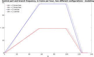
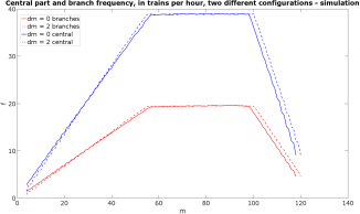
Figure 3: The asymptotic average train frequency $f$ (blue: central part, red: branches), displayed as a function of the number $m$ of moving trains, for the two cases of $\Delta m=0$ (solid line) and $\Delta m=2$ (dashed line). On the left side: analytically derived formula (Corollary 1). On the right side: simulation.

Corollary 1

The average train frequency $f_{0}$ on the central part and $f_{1}=f_{2}$ on the branches are given as follows:

$$f_{0}=2f_{1}=2f_{2}=\max\left\{0,\min\left\{\frac{1}{h_{fw}},\frac{1}{h_{\min}},\frac{1}{h_{bw}},\frac{1}{h_{br}}\right\}\right\}.$$

Proof:

Directly from Theorem 2, with $0\leq f=1/h$. ∎

Theorem 2 shows that in a metro line system with a junction and two symmetrically operated branches, the part with the longest time-headway imposes its frequency to the rest of the system (with the frequency on the branches being half the one on the central part).

We depict in Figure 4 the analytically derived traffic phases of the train dynamics. These frequencies are piecewise linear (Theorem 2 and Corollary 1). RATP, the metro operator of Paris, France, has provided the real values of the minimum running, dwell and safe separation times of a metro line with a junction. Eight traffic phases can be distinguished. The frequencies of the traffic phases in Figure 4, represent the central part of the line. A detailed explanation of the phases will be given in a further paper.

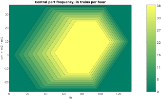
Figure 4: The asymptotic average train frequency $f_{0}$, as a function of the number $m$ of trains on the line and of the difference $\Delta m$ of the number of trains on the two branches. We recognize the eight traffic phases of Theorem 2 and Corollary 1.

We can see, that for every $m$, it exists a $\Delta m$ which maximizes the frequency (Theorem 3):

Theorem 3

$\forall m,\exists\Delta m,f(m,\Delta m)\geq f(m,\Delta m^{\prime}),\forall\Delta m^{\prime}$.

Theorem 3 is an important result and will be used in our further research for traffic control.

Figure 3 illustrates the traffic phases, derived by Theorem 2 and Corollary 1, for two different values of $\Delta m$ on the studied metro line with a junction in Paris, France. On the left side, the analytically derived results are given. On the right side, we show the results from numerical simulations, for comparison. Notice that the analytical derivation and the simulation are coherent. Furthermore, for $m=52$ and $\Delta m=2$, the time-headway (and the frequency) of our model represents precisely the timetable of the line.

To illustrate the impact of the parameter $\Delta m$ on the average asymptotic frequency, we give another configuration, $\Delta m=0$. Let us notice, that on this line, for $m=52$, $\Delta m=2$ maximizes the average asymptotic frequency accordingly to Theorem 3 (proof not given here).

VI Conclusion and future work

These first results of our Max-plus approach to model the dynamical behavior in a metro line system with a junction are encouraging. We will further develop the model towards dynamic dwell times in order to take into account the passenger demand on the platforms and in the trains, as well as dynamic running times to recover perturbations and to stabilize the system. Finally, our future work will focus on a real-time version of the model, where the system is optimized under dynamic passenger demand to guarantee stability.

References

- [1] F. Baccelli, G. Cohen, G. J. Olsder and J.-P. Quadrat, Synchronization and linearity : an algebra for discrete event systems. John Wiley and Sons, 1992.
- [2] Valentina Cacchiani, Dennis Huisman, Martin Kidd, Leo Kroon, Paolo Toth, Lucas Veelenturf, Joris Wagenaar, An Overview of Recovery Models and Algorithms for Real-time Railway Rescheduling. Transportation Research Part B. Volume 63, Pages 15-37, 2014.
- [3] J. Cochet-Terrasson, G. Cohen, S. Gaubert, M. McGettrick, J.-P. Quadrat, Numerical computation of spectral elements in maxplus algebra. In: IFAC Conference on System Structure and Control, Nantes, France, 1998.
- [4] Nadir Farhi, Cyril Nguyen Van Phu, Habib Haj-Salem, Jean-Patrick Lebacque, Traffic modeling and real-time control for metro lines. arXiv preprint arXiv:1604.04593, 2016.
- [5] Nadir Farhi, Cyril Nguyen Van Phu, Habib Haj-Salem, Jean-Patrick Lebacque, Traffic modeling and real-time control for metro lines. Part I - A Max-plus algebra model explaining the traffic phases of the train dynamics. In: Proceedings of American Control Conference, 2017.
- [6] Nadir Farhi, Cyril Nguyen Van Phu, Habib Haj-Salem, Jean-Patrick Lebacque, Traffic modeling and real-time control for metro lines. Part II - The effect of passengers demand on the traffic phases. In: Proceedings of American Control Conference, 2017.
- [7] Rob M.P. Goverde, Railway timetable stability analysis using max-plus system theory. Transportation Research Part B, Volume 41, Issue 2, Pages 179-201, 2007.
- [8] Shukai Li, Maged M. Dessouky, Lixing Yang, Ziyou Gao, Joint optimal train regulation and passenger flow control strategy for high-frequency metro lines. Transportation Research Part B: Methodological, Volume 99, Pages 113-137, 2017.
- [9] Florian Schanzenbächer, Rémy Chevrier, Nadir Farhi, Fluidification du trafic Transilien : approche prédictive et optimisation quadratique. 17th conference ROADEF. Société Française de Recherche Opérationnelle et d’Aide à la Décision, 2016.