Entropic uncertainty relations for successive generalized measurements

Abstract

We derive entropic uncertainty relations for successive generalized measurements by using general descriptions of quantum measurement within two distinctive operational scenarios. In the first scenario, by merging two successive measurements into one we consider successive measurement scheme as a method to perform an overall composite measurement. In the second scenario, on the other hand, we consider it as a method to measure a pair of jointly measurable observables by marginalizing over the distribution obtained in this scheme. In the course of this work, we identify that limits on one’s ability to measure with low uncertainty via this scheme come from intrinsic unsharpness of observables obtained in each scenario. In particular, for the Lüders instrument, disturbance caused by the first measurement to the second one gives rise to the unsharpness at least as much as incompatibility of the observables composing successive measurement.

1 Introduction

Ever since Heisenberg proposed uncertainty principle under consideration of $\gamma$-ray microscope in [1], the uncertainty principle has become one of the most central concepts in quantum physics. Till now, there have been concatenated debates to find uncertainty relations quantitatively well-formulated to reflect underlying meanings of the uncertainty principle [2]. Among the uncertainty relations, one of the most widely known forms of uncertainty relations may be Robertsons’s relation formulated in terms of statistical variances [3]. This relation was discovered by generalizing Kennard’s relation [4] for a pair of arbitrary observables, which indicates limitations on one’s ability to prepare system being well-localized in position and momentum spaces simultaneously, so-called preparation relation. However, underlying meaning of it is not equivalent to Heisenberg’s first insight that there should be a trade-off between imprecision of an instrument measuring a particle’s position and disturbance of its momentum, which is so-called error-disturbance relation. From the Heisenberg’s perspective, various forms of error-disturbance relation were derived based on state-dependent and state-independent quantifications of error and disturbance in [5, 6] and [7, 8], respectively. Here, the point to note in the course of the quantifications is that successive measurement scheme has played major roles in clarifying meaning of error and disturbance, and with increasing experimental ability to control quantum systems these relations were proved [9, 10] by applying this scheme. Nevertheless, uncertainty relations for successive measurements have received less attentions than they deserve, as discussed in [11, 12].

In the field of quantum information theory, uncertainty relations have been formulated in terms of information-theoretic quantities such as entropy, since they are well-defined as a measure of uncertainty in the sense that they are invariant under relabeling of outcomes and concave functions (refer to [13] for further discussions). This information-theoretic approach has been conducted in both preparation and error-disturbance relations. From the point of preparation relation, entropic uncertainty relations were suggested in [14] and then improved by Massen-Uffink [15]. A generalized version of it is written in the form of [16]

$$H_{\rho}(A)+H_{\rho}(B)\geq c,$$ (1)

where we measure observables $A$ and $B$ described by positive-operator-valued measures (POVM) $\{\hat{A}_{i}\}$ and $\{\hat{B}_{j}\}$ on a quantum system $\hat{\rho}$, respectively. In the relation, the Shannon entropy is denoted by $H(A)=-\sum_{i=1}^{n_{A}}p_{A}(i)\log p_{A}(i)$, where $p_{A}(i)=\text{Tr}[\hat{A}_{i}\hat{\rho}]$ is the probability to obtain $i$-th outcome of a measurement of $A$. The lower bound representing incompatibility between $A$ and $B$ is given by

$$c=-\log\max_{i,j}\|\sqrt{\hat{A}_{i}}\sqrt{\hat{B}_{j}}\|^{2},$$ (2)

where the operator norm is denoted by $\|\hat{C}\|$ meaning the maximal singular value of $\hat{C}$. Here and in the following, we will take logarithm in base 2 according to the information-theoretic convention. From the point of error-disturbance relation, there have been recent works to formulate the relation in terms of entropy in order to obtain operationally meaningful formulation, based on state-dependent [17] and state-independent quantifications [18]. (see [19],[20] for more details.)

Inspired by the Heisenberg’s first insight, entropic uncertainty relations for successive projective measurements were considered in an information-theoretic approach [11],[21]. Subsequently, this approach was developed based on Rényi’s entropies [22] and Tsallis’ entropies [23] for a pair of qubit observables. However, the concept of generalized measurements have not been considered in successive measurement scenario. Therefore, the main purpose of the present work is to generalize the entropic uncertainty relations for the case of POVMs. More specifically, we will focus on deriving entropic uncertainty relations for successive generalized measurements with respect to two scenarios. In the first scenario, we consider a statistical distribution of probabilities $p_{AB}(i,j)$ to obtain sequentially measurement outcomes $i$ and $j$ of the first and the second measurements $A$, $B$, respectively. In the second scenario, we analyze the marginal distributions $p_{A}(i)$ and $p_{B^{\prime}}(j)$ associated with jointly measurable observables $A$ and $B^{\prime}$, respectively. In particular, it was argued that the second scenario can be considered as a general method to measure any pair of jointly measurable quantum observables [24], and further it has special usefulness due to so-called universality of successive measurement [25]. In this regard, the range of its applications becomes broader (see the references in [25]). Additionally, in both scenarios, the effect of unsharpness of observables on entropic uncertainty relations will be discussed by using the quantification of unsharpness previously defined in [26].

This paper is organized in the following way. In Section 2 we will introduce a quantity defined as a measure of unsharpness and clarify explicit mathematical expressions of measuring process. Subsequently, based on these mathematical descriptions, entropic uncertainty relations in the first scenario of successive measurement scheme will be derived in Section 3 with specific examples. In Section 4, the second scenario will be considered to derive entropic uncertainty relations. Finally, we will highlight important points of the results, in Section 5.

2 Preliminaries

In this section, we introduce the basic concepts necessary to generalize the entropic uncertainty relations for the case of POVMs in successive measurement scenarios.

2.1 Measure of unsharpness

Here we introduce the measure of unsharpness which was derived based on entropy in [26]. To begin with, let us clarify notations and terminologies as follows. For a finite $d$-dimensional Hilbert space $\mathcal{H}_{d}$, we denote the vector space of all linear operators on $\mathcal{H}_{d}$ by $\mathcal{L}(\mathcal{H}_{d})$. Any observable $A$ then is generally described by POVM $\{\hat{A}_{i}\}$ which is a set of positive operators $\hat{A}_{i}\in\mathcal{L}(\mathcal{H}_{d})$ obeying the completeness relation, $\sum_{i=1}^{n_{A}}\hat{A}_{i}=\hat{I}$ with the number of outcomes of the measurement $n_{A}$. In a particular case that all POVM elements are given as projections, $A$ is a projection-valued measure (PVM). In this case, the observable $A$ is commonly considered as the description of a measurement with perfect accuracy, and thus is called a sharp observable. On the other hand, if $A$ is not a PVM, it is called an unsharp observable.

To clarify the distinction between the concepts of sharp and unsharp observables, we consider $\hat{A}_{i}$ in the form of spectral decomposition

$$\hat{A}_{i}=\sum_{k=1}^{d}a_{i}^{k}|a_{i}^{k}\rangle\langle a_{i}^{k}|,$$ (3)

where $0\leq a_{i}^{k}\leq 1$ is an eigenvalue corresponding to an eigenvector $|a_{i}^{k}\rangle$. By means of this expression, one can find that the condition for sharp observables is equivalent to the statement that all eigenvalues of $\hat{A}_{i}$ are given by either 0 or 1, i.e. $\forall a_{i}^{k}\in\{0,1\}$, as discussed in [27]. Otherwise, we can say that it is unsharp. This statement gives us the idea that the unsharpness measure should be defined as a function of $a_{i}^{k}$ vanishing only when $a_{i}^{k}$ is 0 or 1. Reflecting this idea, the function can be selected in the form of $h(a_{i}^{k})=-a_{i}^{k}\log a_{i}^{k}$, and by averaging it over all POVM elements the measure of unsharpness is defined as [26]

$$D_{\rho}(A)=\sum_{i=1}^{n_{A}}\sum_{k=1}^{d}\langle a_{i}^{k}|\hat{\rho}|a_{i}^{k}\rangle h(a_{i}^{k}),$$ (4)

which is so-called device uncertainty, where a measurement of $A$ is performed on a quantum system $\hat{\rho}$. As a measure of unsharpness, this quantity possesses essential properties such that $D_{\rho}(A)=0$ for all states if and only if $A$ is a PVM, and $D_{\rho}(A)=H_{\rho}(A)$ for all states if and only if $\hat{A}_{i}=\lambda_{i}\hat{I}$ for all $i$ with $0\leq\lambda_{i}\leq 1$ satisfying $\sum_{i=1}^{n_{A}}\lambda_{i}=1$. With additional properties, the validity of this quantity for the unsharpness measure has been verified on the lines of the previous work [28] in which the unsharpness is characterized based on statistical variance. In particular, an important point is that the device uncertainty gives us a nontrivial lower bound of entropy by itself such that

$$H_{\rho}(A)\geq D_{\rho}(A)\geq\min_{\rho}D_{\rho}(A)\geq-\log\max_{i}\|\hat{A}_{i}\|,$$ (5)

due to the concavity of entropy [29]. Moreover, the minimal device uncertainty can be obtained by diagonalizing $\sum_{i=1}^{n_{A}}\sum_{k=1}^{d}h(a_{i}^{k})|a_{i}^{k}\rangle\langle a_{i}^{k}|$ and taking the lowest eigenvalue, which is stronger than $-\log\max_{i}\|\hat{A}_{i}\|$ proposed in [16]. In other words, this method makes it available for us to generally find stronger state-independent bounds, and thus will play key roles in deriving entropic uncertainty relations for successive measurements. The detailed properties of the device uncertainty $D_{\rho}(A)$ has been studied in [26].

2.2 General description of successive measurements

In the present work, by a successive measurement, we mean a scheme where two measurements are performed one after the other successively. In particular, the second measurement is assumed to be performed immediately on an output state conditionally transformed according to an outcome of the first measurement. Thus, in order to consider successive measurement scheme, we should clarify how input state is transformed to output states conditioned on the measurement outcome. For this purpose, however, the concept of POVM is not enough to fully describe the state transformation. For general description of successive measurements, therefore, we need the concept of an instrument [30], which is a mapping $\mathcal{I}:i\rightarrow\mathcal{I}_{i}$ such that each $\mathcal{I}_{i}$ is a completely positive linear map on $\mathcal{L}(\mathcal{H}_{d})$ satisfying $\sum_{i=1}^{m}\text{tr}[\mathcal{I}_{i}(\hat{\rho})]=1$ for all states $\hat{\rho}$.

A general description of a quantum measurement is given by a pair of an observable $A$ and an instrument. However, a notable point is that for a given $A$ not all instruments are compatible with $A$. For the description to be valid, an instrument should obey the condition that each $i$-th completely positive linear map $\mathcal{I}^{A}_{i}$ satisfies

$$\text{tr}[\mathcal{I}^{A}_{i}(\hat{\rho})]=\text{tr}[\hat{A}_{i}\hat{\rho}]$$ (6)

for all states $\hat{\rho}$, and in this case we say that an instrument $\mathcal{I}^{A}$ is $A$-compatible. Accordingly, $A$-compatible instrument illustrates that a measurement outcome $i$ is obtained with the probability $p^{A}_{i}=\text{tr}[\hat{A}_{i}\hat{\rho}]$ for an input state $\hat{\rho}$, and a normalized output state $\mathcal{I}_{i}^{A}(\hat{\rho})/p_{i}^{A}$ is generated as depicted in Figure 1-(a). Among $A$-compatible instruments, the most common instruments occurring in applications may be the Lüders instrument, defined by

$$\mathcal{I}_{i}^{A_{L}}(\hat{\rho})=\sqrt{\hat{A}_{i}}\hat{\rho}\sqrt{\hat{A}_{i}}.$$ (7)

The Lüders instrument is the generalized version of projective measurements for general POVM, in the sense that for sharp observables it illustrates the same with state transformation of projective measurement.

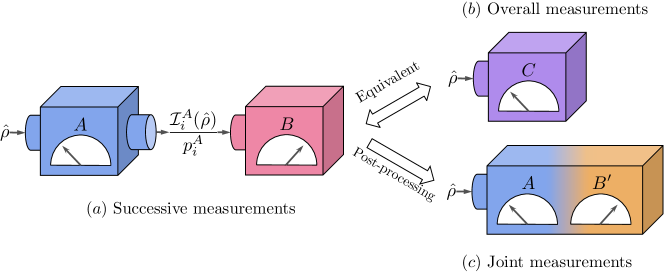
Figure 1: Relations among measurement schemes. (a) Successive measurement of observables $A$ and $B$, where the first measurement $A$ gives rise to output state $\mathcal{I}_{i}^{A}(\rho)/p_{A}(i)$ conditioned on its outcome $i$. (b) Overall measurement of $C$ obtained by performing the successive measurement of $A$ and $B$. (c) Joint measurements obtained in successive measurement scheme by considering the marginal distributions

Additionally, the concept of measuring process deserves consideration in order to describe successive measurement in a more specific way, of which a description is known to be consistent with the description of instrument [31]. A measuring process is defined to be a quadruple $(\mathcal{K},|\xi\rangle,\hat{U},F)$ consisting of a Hilbert space $\mathcal{K}$ associated with a probe system, a state vector $|\xi\rangle$ on $\mathcal{K}$, a unitary operator $\hat{U}$ on $\mathcal{H}\otimes\mathcal{K}$, and an observable $F$ on $\mathcal{K}$. The quadruple $(\mathcal{K},|\xi\rangle,\hat{U},F)$ is compatible with an observable $A$ if it satisfies

$$\text{tr}[\hat{A}_{i}\hat{\rho}]=\text{tr}[\hat{U}(\hat{\rho}\otimes|\xi\rangle\langle\xi|)\hat{U}^{\dagger}(\hat{I}\otimes\hat{D}_{i})]$$ (8)

for all $i$ and states. It means that the measuring process for $A$ gives rise to the same with a probability distribution obtained by performing a measurement of $A$ directly on the system. In this case, an instrument $\mathcal{I}^{A}$ is related to the measuring process $(\mathcal{K},|\xi\rangle,\hat{U},F)$ in the following manner

$$\mathcal{I}^{A}_{i}(\hat{\rho})=\text{tr}_{\mathcal{K}}[\hat{U}(\hat{\rho}\otimes|\xi\rangle\langle\xi|)\hat{U}^{\dagger}(\hat{I}\otimes\hat{F}_{i})]$$ (9)

for all $i$ and states. In this way, each measuring process defines a unique instrument and conversely for every instrument there exists a measuring process explicitly describing the same state transformation [31]. We refer to [32] for more details.

Based on the above mathematical descriptions, there are two scenarios to investigate statistical properties of a distribution obtained in the successive measurement scheme. Now, let us consider the first scenario in which we sequentially perform two measurements $A$ and $B$ as depicted in Figure 1-(a), where the numbers of measurement outcomes are $n_{A}$ and $n_{B}$, respectively. Then, this scenario can be seen as a method to obtain the overall observable $C$ described by POVM $\{\hat{C}_{ij}\}$ obeying

$$\text{tr}[\hat{C}_{ij}\hat{\rho}]=\text{tr}[\mathcal{I}^{A}_{i}(\hat{\rho})\hat{B}_{j}]=p_{AB}(i,j)$$ (10)

for all $i,j$ and all states $\hat{\rho}$. In the Heisenberg picture, equivalently, it can be rewritten as

$$\hat{C}_{ij}=\mathcal{I}^{A*}_{i}(\hat{B}_{j}),$$ (11)

where $\mathcal{I}^{A*}_{i}$ denotes the adjoint map of $\mathcal{I}^{A}_{i}$. As illustrated in Figure 1-(b), namely, the successive measurements $A$, $B$ are merged into $C$ having $n_{A}n_{B}$ outcomes. Consequently, a task to analyze statistical properties in the successive measurements can be accomplished by exploring the overall observable $C$ without loss of generality. In this approach, we will investigate the entropic uncertainty relation in Section 3.

On the other hand, in the second scenario we take into account the marginal distributions obtained as $\sum_{j=1}^{n_{B}}p_{AB}(i,j)=p_{A}(i)$ and $\sum_{i=1}^{n_{A}}p_{AB}(i,j)=p_{B^{\prime}}(j)$. Namely, the successive measurement scheme is considered as a strategy to perform a joint measurement of $A$ and $B^{\prime}$ as depicted in Figure 1-(c), where the observables $A$ and $B^{\prime}$ are described by

$$\hat{A}_{i}=\sum_{j=1}^{n_{B}}\hat{C}_{ij}\;\;\;\;\;\text{ and }\;\;\;\;\;\hat{B}^{\prime}_{j}=\sum_{i=1}^{n_{A}}\hat{C}_{ij}$$ (12)

for all $i$, $j$, respectively. It is worth noting that performing the second measurement $B$ is effectively equivalent to perform the measurement $B^{\prime}$ on the initial system, since the first measurement disturbs the second one. However, it has been shown that, despite of this disturbance, any jointly measurable pair of quantum observables can be measured by means of successive measurement scheme [24]. Therefore, considering the second scenario is a general way to explicitly explore the concept of jointly measurable observables. Entropic uncertainty relations in this scenario will be taken into account in Section 4.

3 Generalized version of entropic uncertainty relation for successive measurements

In the previous section, the mathematical methods have been presented, which are necessary to describe successive measurement in general. Based on the methods, we derive entropic uncertainty relations within the first scenario. As mentioned in Section 2.2, we can consider performing successive measurement of $A$ and $B$ as a method to implement the corresponding overall measurement of $C$. This fact implies that uncertainty existing in this scenario can be equivalently characterized as entropy of $C$,

$$H_{\rho}(A,B)=H_{\rho}(C),$$ (13)

since $p_{AB}(i,j)=p_{C}(i,j)$ for all $i$, $j$. In other words, our goal to analyze uncertainty existing in the first scenario can be achieved under consideration of the overall observable $C$. From this point of view, one can identify that the reason why we cannot avoid uncertainty in this scheme originates from intrinsic unsharpness of the overall observable $C$. By quantitatively formulating this fact, as described in Equation (5), we obtain entropic form of uncertainty relation lower bounded by device uncertainty characterizing unsharpness of $C$ such that

$$H_{\rho}(A,B)\geq D_{\rho}(C)\geq\min_{\rho}D_{\rho}(C)\equiv\mathcal{D}_{1},$$ (14)

where state-independent bound $\mathcal{D}_{1}$ is obtained by minimizing device uncertainty of $C$ over all states. An important point here is that sequentially measuring incompatible observables may give rise to unavoidable unsharpness as the second measurement is disturbed by performing the first one. We can clearly observe the phenomena in the following cases.

3.1 Projective measurement model

In order to examine how much unsharpness emerges due to the incompatibility in the first scenario, let us consider successive projective measurements of observables $A$ and $B$ described by orthonormal bases $\{|a_{i}\rangle\}$ and $\{|b_{j}\rangle\}$ in $\mathcal{H}_{d}$, respectively. Then, according to the state transformation $\mathcal{I}_{i}^{A}(\rho)=\langle a_{i}|\hat{\rho}|a_{i}\rangle|a_{i}\rangle\langle a_{i}|$, this successive measurement can be considered as the overall measurement of $C$, which is described by

$$\hat{C}_{ij}=|\langle a_{i}|b_{j}\rangle|^{2}|a_{i}\rangle\langle a_{i}|$$ (15)

for all $i$, $j$. In this case, by calculating the minimal value of device uncertainty defined in Equation (5) we obtain

$$H_{\rho}(A,B)\geq\min_{i}\left(-\sum_{j=1}^{d}|\langle a_{i}|b_{j}\rangle|^{2}\log|\langle a_{i}|b_{j}\rangle|^{2}\right),$$ (16)

where the lower bound was proposed in [11]. Here, it is notable that this bound is stronger than $-\log\max_{i,j}|\langle a_{i}|b_{j}\rangle|^{2}$, which is widely known as a measure of incompatibility [15]. Thus, successively performing projective measurements of incompatible sharp observables induces unavoidable unsharpness which gives limits on one’s ability to measure with arbitrarily low uncertainty.

3.2 Lüders instrument

As a generalized version of projective measurement model, let us assume that we implement the Lüders instrument for an unsharp observable $A$ at first and later a measurement of $B$ in the first scenario. In this case, each map $\mathcal{I}_{i}^{A_{L}}$ is fully determined by POVM element $\hat{A}_{i}$ as defined in Equation (7), so that by applying adjoint map of $\mathcal{I}^{A_{L}}_{i}$ to each POVM element of $B$ such as Equation (11), we obtain the explicit form of the overall observable $C$ described by

$$\hat{C}_{ij}=\sqrt{\hat{A}_{i}}B_{j}\sqrt{\hat{A}_{i}}$$ (17)

for all $i$, $j$. Then, it is straightforward to formulate relations among the concepts of uncertainty, unsharpness and incompatibility by directly using the relations in Equation (5)

$$H_{\rho}(A,B)\geq\mathcal{D}_{1}\geq-\log\max_{i,j}\|\sqrt{\hat{A}_{i}}B_{j}\sqrt{\hat{A}_{i}}\|=c.$$ (18)

Here, the last inequality in Equation (18) means that the minimal value of device uncertainty gives rise to a stronger bound than the incompatibility $c$ defined in Equation (2). Therefore, as observed in the case of projective measurement model, one can identify that measuring incompatible observables by means of the Lüders instrument imposes the unavoidable unsharpness. In the following examples, we will analyze the relationships in Equation (18).

3.3 Examples in spin $\frac{1}{2}$ system

   

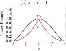
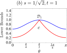
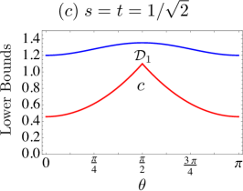
Figure 2: Graphs illustrate the lower bounds in Equation (14) for successive measurement of $Z$ and $X(\theta)$ with respect to angle $\theta$. Varying unsharpness of the observables, we present three cases. (a) At $s=t=1$, both observables are sharp. (b) At $s=1/\sqrt{2},t=1$, only the first one is unsharp. (c) At $s=t=1/\sqrt{2}$, both are unsharp.

In order to clarify the relationship between $\mathcal{D}_{1}$ and $c$ and verify the validity of $\mathcal{D}_{1}$ for lower bound of uncertainty relation (18), let us consider an example of successively measuring two spin observables $Z$ at first and $X(\theta)$ later in $\mathcal{H}_{2}$ described by

$$\hat{Z}_{\pm}=\frac{\hat{I}\pm s\hat{\sigma}_{z}}{2}\;\;\;\;\;\;\text{ and }\;\;\;\;\;\;\hat{X}_{\pm}(\theta)=\frac{\hat{I}\pm t(\sin\theta\hat{\sigma}_{x}+\cos\theta\hat{\sigma}_{z})}{2},$$ (19)

respectively, where $\hat{\sigma}_{x}$ and $\hat{\sigma}_{z}$ are the Pauli spin matrices and unsharp parameters are denoted by $0\leq s,t\leq 1$. Then the incompatibility of the observables is determined by $\theta$ which is angle between directions of measurement components. Additionally, we assume that a $Z$-compatible instrument is induced by a measuring process $(\mathcal{H}_{2},|\phi\rangle,\hat{U}_{CNOT},\sigma_{z})$, where an initial state of the probe system is $|\phi\rangle=\sqrt{(1+s)/2}|0\rangle+\sqrt{(1-s)/2}|1\rangle$ and a unitary operator $\hat{U}_{CNOT}$ gives rise to a CNOT gate controlled by eigenstates of $\hat{\sigma}_{z}$, $|0\rangle$ and $|1\rangle$. Namely, this measuring process leads to the Lüders instrument for $Z$. In this case, the successive measurement scheme is equivalent to perform the overall measurement of $S$ defined in terms of four POVM elements

$$\hat{S}_{\pm\pm}=\frac{1}{4}\Big{(}(1+st\cos\theta)\hat{I}\pm\sqrt{1-s^{2}}t\sin(\theta)\;\hat{\sigma}_{x}\pm(s+t\cos\theta)\hat{\sigma}_{z}\Big{)},$$ (20)

$$\hat{S}_{\pm\mp}=\frac{1}{4}\Big{(}(1-st\cos\theta)\hat{I}\mp\sqrt{1-s^{2}}t\sin(\theta)\;\hat{\sigma}_{x}\pm(s-t\cos\theta)\hat{\sigma}_{z}\Big{)}.$$ (21)

Calculating the device uncertainty for the overall observable $S$, we obtain state-independent lower bounds

$$\mathcal{D}_{1}=\sum_{\begin{subarray}{c}\mu=\pm 1\\ \nu=\pm 1\end{subarray}}h\left(\frac{1}{4}\left(1+\mu st\cos\theta+\nu\sqrt{s^{2}+t^{2}+\mu 2st\cos\theta+s^{2}t^{2}(\cos^{2}\theta-1)}\right)\right).$$ (22)

We plot the lower bounds $\mathcal{D}_{1}$ and

$$c=-\log\Big{(}\frac{1}{4}(1+st|\cos\theta|+\sqrt{s^{2}+t^{2}+2st|\cos\theta|+s^{2}t^{2}(\cos^{2}\theta-1)})\Big{)}$$

presented in Equation (14) versus the angle $\theta$. As a result, we can check that $\mathcal{D}_{1}$ gives rise to strictly stronger bound than $c$ except when the spin components are mutually parallel or perpendicular in Figure 2-(a). With increasing unsharpness of the observables, it becomes evident that $\mathcal{D}_{1}$ is well-formulated to reflect the effect of unsharpness as observed in Figures 2-(b), (c). In the examples, we analytically confirm the validity of $\mathcal{D}_{1}$ for a lower bound by comparing with $c$, and, as a result, observe that measuring incompatible observables gives rise to unavoidable unsharpness originating from the incompatibility on the assumption that we implement the Lüders instrument in the first scenario.

4 Entropic uncertainty relations for a jointly measurable pair of observables obtained via successive measurement scheme

In this section, we consider entropic uncertainty relations for a pair of jointly measurable observables obtained via successive measurement scheme within the second scenario. As a first step, let us clarify the concept of a joint measurement. Given observables $A$ and $B$, they are jointly measurable if and only if there exists a joint observable $M$ composed of $n_{A}n_{B}$-elements of POVM satisfying [33]

$$\sum_{j=1}^{n_{B}}\hat{M}_{ij}=\hat{A}_{i}\;\;\;\text{and}\;\;\;\sum_{i=1}^{n_{A}}\hat{M}_{ij}=\hat{B}_{j}.$$ (23)

Specifically, in the second scenario, the overall observable $C$ can be seen as a joint observable of $A$ and $B^{\prime}$ by the definitions (12). Moreover, as mentioned in Section 2.2, this scheme generally provides a method to implement joint measurements of any jointly measurable observables [24]. Hence, entropic uncertainty relations obtained within this scenario is applicable to any pair of them.

Both observables $A$ and $B^{\prime}$ obtained via the second scenario may have their own unsharpness, so that an amount of uncertainties about $A$ and $B^{\prime}$ may not vanish due to the unsharpness of them. As formulating this fact, we obtain entropic uncertainty relations within the second scenario in the form of

$$H_{\rho}(A)+H_{\rho}(B^{\prime})\geq D_{\rho}(A)+D_{\rho}(B^{\prime})\geq\min_{\rho}\left[D_{\rho}(A)+D_{\rho}(B^{\prime})\right]\equiv\mathcal{D}_{2},$$ (24)

where the sum of device uncertainties is written as

$$D_{\rho}(A)+D_{\rho}(B^{\prime})=\text{tr}\left[\hat{\rho}\left(\sum_{i=1}^{n_{A}}\sum_{k=1}^{d}h(a_{i}^{k})|a_{i}^{k}\rangle\langle a_{i}^{k}|+\sum_{j=1}^{n_{B}}\sum_{l=1}^{d}h({b^{\prime}}_{j}^{l})|{b^{\prime}}_{j}^{l}\rangle\langle{b^{\prime}}_{j}^{l}|\right)\right],$$ (25)

and thus minimizing it over all states can be accomplished by diagonalizing

$$\big{(}\sum_{i=1}^{n_{A}}\sum_{k=1}^{d}h(a_{i}^{k})|a_{i}^{k}\rangle\langle a_{i}^{k}|+\sum_{j=1}^{n_{B}}\sum_{l=1}^{d}h({b^{\prime}}_{j}^{l})|{b^{\prime}}_{j}^{l}\rangle\langle{b^{\prime}}_{j}^{l}|\big{)}$$

and taking the lowest eigenvalue. An important point, here, is that the second measurement $B$ may be perturbed to be $B^{\prime}$ because of disturbance caused by the first measurement $A$, while $A$ is preserved. This fact implies that even when both observables $A$ and $B$ applied in this scheme are sharp, it is possible for the perturbed one $B^{\prime}$ to become unsharp. In particular, this behavior is apparently observed when applying a pair of incompatible observables to this scenario, since measuring one of a pair of incompatible observables disturbs the other, according to the Heisenberg’s insight. From the point of view that the incompatibility imposes unavoidable unsharpness on the observables $A$ and $B^{\prime}$, we will discuss more details in the following specific measurement models.

4.1 Projective measurement model

In the same way in Section 3.1, let us consider projective measurements of $A$ and $B$ described in $\mathcal{H}_{d}$ by orthonormal bases $\{|a_{i}\rangle\}$ and $\{|b_{j}\rangle\}$, respectively. Then, in the second scenario, the first one $A$ remains itself, while the second one $B$ is disturbed to be $B^{\prime}$ described by

$$\hat{B}_{j}^{\prime}=\sum_{i=1}^{d}|\langle a_{i}|b_{j}\rangle|^{2}|a_{i}\rangle\langle a_{i}|$$ (26)

for all $j$. According to the Lüders theorem [34], $B$ is not disturbed if and only if all elements of $A$ and $B$ commute each other. In this case, thus, even though we perform two sharp observables sequentially, the second one involves the unavoidable unsharpness originating from the incompatibility between them. This behavior can be quantitatively formulated in the form of

$$H_{\rho}(A)+H_{\rho}(B^{\prime})\geq D_{\rho}(B^{\prime})\geq\min_{\rho}D_{\rho}(B^{\prime})=\min_{i}\left(-\sum_{j=1}^{d}|\langle a_{i}|b_{j}\rangle|^{2}\log|\langle a_{i}|b_{j}\rangle|^{2}\right),$$ (27)

where its lower bound was proposed in [11]. Generalized version of it for POVMs will be taken into account in the following.

4.2 Lüders instruments

As a next step, in the same manner as Section 3.2, let us assume we sequentially implement the Lüders instrument of an observable $A$ at first and later another one of $B$, in the second scenario. Then, according to Equation (7), it is equivalent to implement joint measurement of a pair of observables $A$ and $B^{\prime}$ described by

$$\hat{A}_{i}\;\;\;\;\;\text{ and }\;\;\;\;\;\hat{B}^{\prime}_{j}=\sum_{i=1}^{n_{A}}\sqrt{\hat{A}_{i}}\hat{B}_{j}\sqrt{\hat{A}_{i}},$$ (28)

for all $i$, $j$, respectively. In this case, likewise as discussed above, performing the Lüders instrument of $A$ gives rise to disturbance to $B$, in a way for $B$ to become $B^{\prime}$. Then, by applying the relations in Equation (5) directly, we obtain

$$H_{\rho}(A)+H_{\rho}(B^{\prime})\geq D_{\rho}(A)+D_{\rho}(B^{\prime})\geq\min_{\rho}\left[D_{\rho}(A)+D_{\rho}(B^{\prime})\right]\geq-\log\max_{j}\|\sum_{i=1}^{n_{A}}\sqrt{\hat{A}_{i}}\hat{B}_{j}\sqrt{\hat{A}_{i}}\|,$$ (29)

where the last inequality follows from applying the third inequality in Equation (5) solely to the observable $B^{\prime}$ and its bound is a new form of incompatibility larger than $-\log\max_{i,j}\|\sqrt{\hat{A}_{i}}\sqrt{\hat{B}_{j}}\|^{2}$, which was conjectured in [35] and proved later in [36]. A distinct point from projective measurement model is that there is a possibility for $A$ to be unsharp, and loosing sharpness of $A$ may decrease disturbance to $B$ caused by $A$. Namely, a trade-off between the unsharpness of $A$ and $B$ can be observed. In the following examples, this phenomenon will be examined.

4.3 Examples in spin $\frac{1}{2}$ system

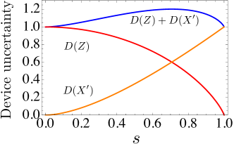
Figure 3: For a pair of jointly measurable observables $Z$ and $X^{\prime}$ obtained via successive measurement scheme, we plot device uncertainties of them and their summation denotes by $D(Z)$, $D(X^{\prime})$ and $D(Z)+D(X^{\prime})$, respectively, versus the unsharp parameter $s$. We can observe trade-off relation between $D(Z)$ and $D(X^{\prime})$ characterizing unsharpness of $Z$ and $X^{\prime}$.

As an example in the second scenario, we assume to implement the Lüders instrument of $Z$ induced by the measuring process $(\mathcal{H}_{2},|\phi\rangle,\hat{U}_{CNOT},\sigma_{z})$ and a measurement of $X$ successively in $\mathcal{H}_{2}$ described by

$$\hat{Z}_{\pm}=\frac{\hat{I}\pm s\hat{\sigma}_{z}}{2}\;\;\;\;\;\;\text{ and }\;\;\;\;\;\;\hat{X}_{\pm}=\frac{\hat{I}\pm\hat{\sigma}_{x}}{2},$$ (30)

respectively. Here we restrict ourselves for $X$ to be sharp, in order to observe more clearly unsharpness appearing due to the first measurement. In this case, we can consider it as a method to measure a pair of jointly measurable observables $Z$ and $X^{\prime}$, where the perturbed observable $X^{\prime}$ is given as [37]

$$\hat{X}^{\prime}_{\pm}=\frac{\hat{I}\pm t\hat{\sigma}_{x}}{2}$$ (31)

with the unsharp parameter $t=\sqrt{1-s^{2}}$. Consequently, this scheme provides an optimized method to jointly measure incompatible observables $\sigma_{z}$ and $\sigma_{x}$, in the sense that the unsharp parameters $s$ and $t$ saturate the inequality $s^{2}+t^{2}\leq 1$, which is a necessary and sufficient condition for $Z$ and $X^{\prime}$ to be jointly measurable [38]. However, even in the optimized method, we can not avoid unsharpness, and there is the trade-off between the unsharpness of $Z$ and $X^{\prime}$ such that the more sharpness of $Z$, the more unsharpness of $X^{\prime}$. This behavior can be examined quantitatively by considering entropic uncertainty relations (24) given in the form of

$$H_{\rho}(Z)+H_{\rho}(X^{\prime})\geq D(Z)+D(X^{\prime})=H_{bin}\left(\frac{1+s}{2}\right)+H_{bin}\left(\frac{1+\sqrt{1-s^{2}}}{2}\right),$$ (32)

where binary entropy is denoted by$H_{bin}(q)=-h(q)-h(1-q)$. The trade-off between the unsharpness of them is illustrated in Figure 3, and the total unsharpness characterized by $D(Z)+D(X^{\prime})$ is maximized when unsharpness equally distributed $s=t=1/\sqrt{2}$, while minimized at extreme points $s=1$ or $s=0$.

5 Conclusion

The main purpose of present work is to suggest entropic uncertainty relations for successive generalized measurement within two distinctive scenarios. Before deriving the relations, in Section 2, we have introduced device uncertainty as a measure of unsharpness and its mathematical properties in order to investigate the effect of unsharpness on entropic uncertainty relations in successive measurement scheme. Subsequently, we have explicitly explained general description of successive measurement scheme with respect to two scenarios. In the first scenario, we have considered this scheme as a method to implement an overall measurement, and, as a result, observed that unsharpness of the overall observable gives limits on one’s ability to measure it with arbitrarily low uncertainty as formulated in Equation (14). Assuming to perform the Lüders instrument as the first measurement in this scenario, it is clearly shown that this unsharpness comes from disturbance caused by the first measurement to the second one. The amount of unsharpness appears at least as much as the incompatibility of a pair of observables composing successive measurement, as formulated in Equation (18). In the second scenario, on the other hand, this scheme has been considered as a method to measure a pair of jointly measurable observables. Consequently, we have figured out that total unsharpness in both observables is a major factor that gives rise to unavoidable uncertainty as observed in Equation (24). Also under the assumption for the first measurement to be described by the Lüders instrument, it becomes clear that the first measurement leads to unsharpness of the second one by disturbing it at least as much as incompatibility as shown in Equation (29). It is notable that this form of uncertainty relations is applicable to any pair of jointly observables, since Heinosaari et al. have proved that we can obtain any pair of jointly measurable observables via successive measurement scheme in [24].

Abbreviations

The following abbreviations are used in this manuscript:

POVM: Positive Operator Valued Measure
PVM: Projector Valued Measure

References

- [1] Heisenberg, W. Über den anschulichen Inhalt der quantentheoretischen Kinematik und Mechanik. Z. Phys. 1927 43, 172-198.
- [2] Busch, P.; Heinosaari, T.; Lahti, P. Heisenberg’s uncertainty principle. Physics Reports 2007 452, 155-176.
- [3] Robertson, H. P. The uncertainty principle Phys. Rev. 1929 34, 163.
- [4] Kennard, E.H. Zur Quantenmechanik einfacher Bewegungstypen. Z. Phys. 1927, 44, 326-352
- [5] Ozawa, M. Universally valid reformulation of the Heisenberg uncertainty principle on noise and disturbance in measurement, Phys. Rev. A 2003, 67, 042105.
- [6] Branciard, C. Error-tradeoff and error-disturbance relations for incompatible quantum measurements Proc. Nat. Acad. Sci. 2013 110, 6742-6747.
- [7] Busch, P.; Lahti, P.; Werner, R. F. Proof of Heisenberg’s error-disturbance relation, Phy. Rev. Lett. 2013 111, 160405.
- [8] Busch, P.; Lahti, P.; Werner, R. F. Heisenberg uncertainty for qubit measurements Phy. Rev. A 2014 89, 012129.
- [9] Erhart, J.; Spona, S.; Sulyok, G.; Badurek, G.; Ozawa, M.; Yuji, H. Experimental demonstration of a universally valid error-disturbance uncertainty relation in spin measurements. Nature Phys. 2012 8, 185-189.
- [10] Rozema, L. A.; Darabi, A.; Mahler, D. H.; Hayat, A.; Soudagar, Y.; Steinberg, A. M. Violation of Heisenberg’s measurement-disturbance relationship by weak measurements. Phys. Rev. Lett. 2012 109, 100404.
- [11] Srinivas, M. D. Optimal entropic uncertainty relation for successive measurements in quantum information theory Paramana-J. Phys. 2002 60 1137-1152.
- [12] Distler, J.; Paban, S. Uncertainties in successive measurements Phy. Rev. A 2013 87, 062112.
- [13] Uffink, J.B.M. Measures of Uncertainty and the Uncertainty Principle, Ph.D. thesis, University of Utrecht, Utrecht, Netherlands,1990.
- [14] Deutsch, D. Uncertainty in Quantum Measurements Phy. Rev. Lett. 1983 50, 631.
- [15] Maasen, H.; Uffink, J.B.M. Generalized entropic uncertainty relations Phy. Rev. Lett. 1988 60, 1103-1106.
- [16] Krishna M.; Parthasarathy, K.R. An entropic uncertainty principle for quantum measurements Indian J. Stat. Ser. A 2002 64, 842
- [17] Coles, P.J.; Furrer, F. State-dependent approach to entropic measurement-disturbance relations. Physics Letters A 2015 379 105-112
- [18] Buscemi, F.; Hall, M.J.W.; Ozawa, M.; Wilde, M.M. Noise and disturbance in quantum measurements: An information-theoretic approach. Phys. Rev. Lett. 2014 112, 050401.
- [19] Wehner, S.; Winter, A. Entropic uncertainty relations-a survey New. J. Phys. 2010 12, 025009.
- [20] Coles, P.J.; Berta, M.; Tomamichel, M.; Wehner, S. Entropic uncertainty relations and their applications. Rev. Mod. Phys. 2017 89, 015002.
- [21] Baek, K.; Farrow, T.; Son, W. Optimized entropic uncertainty for successive projective measurements Phys. Rev. A 2014 89, 032108.
- [22] Zhang, L; Zhang, Y.; Yu, C. Rényi entropy uncertainty relation for successive projective measurements. Quantum Information Processing, 2015 14, 2239-2253.
- [23] Rastegin, A.E. Uncertainty and certainty relations for successive projective measurements of a qubit in terms of Tsallis’ tntropies. Commun. Theor. Phys. 2015 63, 687.
- [24] Heinosaari, T.; Wolf, M. Non-disturbing quantum measurements. J. Math. Phys. 2010 51, 092201.
- [25] Heinosaari, T.; Miyadera, T. Universality of sequential quantum measurements Phys. Rev. A 2015 91, 022110.
- [26] K. Baek, W. Son, Unsharpness of generalized measurement and its effects in entropic uncertainty relations. Sci. Rep. 2016, 6, 30228
- [27] Busch, P. On the sharpness and bias of quantum effects. Found. Phys. 2009 39, 712.
- [28] Massar, S. Uncertainty relations for positive-operator-valued measures. Phys. Rev. A 2007 76, 042114.
- [29] Cover, T.M. and Thomas, J.A. Elements of Information Theory; Wiley: New York, USA, 1991.
- [30] Davies, E.B. Quantum theory of open systems; Academic Press: London, UK, 1976.
- [31] Ozawa, M. Conditional expectation and repeated measurements of continuous quantum observables. J. Math. Phys. 1984 25, 79-87
- [32] Heinosaari, T. and Ziman, M. The mathematical language of quantum theory from uncertainty to entanglement; Cambridge University Press: Cambridge, UK, 2012.
- [33] Lahti, P.; Pulmannová, S. Coexistent observables and effects in quantum mechanics. Rep. Math. Phys. 1997 39, 339.
- [34] Lüders, G. Über die Zustandsänderung durch den Messprozess. Ann. Physik (6), 1951 8, 322–328.
- [35] Tomamichel, M. A Framework for Non-Asymptotic Quantum Information Theory, Ph.D. thesis, ETH Zurich, Zurich, Switzerland, 2012.
- [36] Coles, P.J.; Piani, M. Improved entropic uncertainty relations and information exclusion relations. Phys. Rev. A, 2014 89, 022112.
- [37] Carmeli, C.; Heinosaari, T.; Toigo, A. Informationally complete joint measurements on finite quantum systems. Phys. Rev. A 2012 85, 012109.
- [38] Busch, P. Unsharp reality and joint measurements for spin observables. Phys. Rev. D, 1986 33, 2253.