Mass, energy, and momentum capture from stellar winds by magnetized and unmagnetized planets: implications for atmospheric erosion and habitability

Abstract

The extent to which a magnetosphere protects its planetary atmosphere from stellar wind ablation depends upon how well it prevents energy and momentum exchange with the atmosphere and how well it traps otherwise escaping plasma. We focus on the former, and provide a formalism for estimating approximate upper limits on mass, energy, and momentum capture, and use them to constrain loss rates. Our approach quantifies a competition between the local deflection of incoming plasma by a planetary magnetic field and the increase in area for solar wind mass capture provided by this magnetosphere when the wind and planetary fields incur magnetic reconnection. Solar wind capture can be larger for a magnetized planet versus an unmagnetized planet with small ionosphere, even if the rate of energy transfer is less. We find this to be the case throughout Earth’s history since the lunar forming impact– the likely start of the geodynamo. Focusing of incoming charged particles near the magnetic poles can increase the local energy flux for a strong enough planetary field and weak enough wind, and we find that this may be the case for Earth’s future. The future protective role of Earth’s magnetic field would then depend on its ability to trap outgoing plasma. This competition between increased collection area and reduced inflow speed from a magnetosphere is likely essential in determining the net protective role of planetary fields and its importance in sustaining habitability, and can help explain the current ion loss rates from Mars, Venus and Earth.

1 Introduction

Traditionally, planetary habitable zones are defined as the range of distances from a star within which a planet can orbit such that stellar luminosity heats the planet to a temperature range that can sustain gravitationally bound liquid water (Huang, 1960; Kasting, Whitmire & Reynolds, 1993). However, even if liquid water is essential, the potentially catastrophic effect of stellar activity from ultraviolet and X-ray photons, and stellar winds on the planetary atmosphere must also be considered (e.g. Lammer, 2013). High energy photons can photo-dissociate molecules and/or heat atoms such that that the atmospheric constituents exceed the escape speed at the exobase and are catastrophically lost. Complementarily, a strong stellar wind can exchange momentum with the planetary atmosphere and directly or indirectly eject the essential constituents.

The overall effects of stellar activity on atmospheres are commonly (if not misleadingly) delineated as “thermal” or “non-thermal” mechanisms (e.g. Hunten, 1982; Kumar, Hunten & Pollack, 1983; Kasting & Pollack, 1983; Shizgal & Arkos, 1996; Lammer & Bauer, 1991; Hunten, 1993; Seager, 2010; Lammer, 2013). For the former, energy is primarily absorbed and converted to thermal energy. The potential for ejection amounts to a comparison between thermal velocities and escape speed. Non-thermal mechanisms refer to those in which the input energy is not thermalized by collisions and/or may involve a change of chemistry or ionization state of the influenced particles. Erosion of atmospheres by stellar winds is an important example of the latter, and the focus of the present paper. Ultimately, a realistic determination of habitability will depend on understanding the high energy coronal activity from stars and the efficacy with which planetary atmospheres are protected against the associated radiation and winds.

The magnetic field strength and X-ray activity of solar-like stars increase with rotation rate for slow rotators and then saturate for very fast rotators (Noyes et al., 1984; Schrijver & Zwaan, 2000; Pizzolato et al., 2003; Mamajek & Hillenbrand, 2008; Wright et al., 2011; Vidotto et al., 2014; Reiners, Schüssler & Passegger, 2014). Relationships between stellar activity, rotation, and magnetic field strength are all connected to the dynamo origin of these fields within the stars; it is an ongoing enterprise of research to understand these connections and make them quantitative (Karak, Kitchatinov & Choudhuri, 2014; Kitchatinov & Olemskoy, 2015; Sood, Kim & Hollerbach, 2016; Blackman & Owen, 2016). In the absence of significant cooling, the winds from solar-like stars, which also draw from the coronal magnetic and thermal energy, are also likely significantly stronger for younger stars. This too, however, is debated and a topic of active research (Wood, 2006; Wood et al., 2014; Cohen, 2011; Suzuki et al., 2013; Matt et al., 2015; Blackman & Owen, 2016).

Planetary magnetospheres produced from core dynamos are widely perceived to be protective against erosion from stellar winds. This is of topical interest in understanding the evolution of the early Earth (Tarduno et al., 2015) and well as the potential habitability of exoplanets (do Nascimento et al., 2016). The planetary magnetic field acts as a magnetic cage that tempers stripping by stellar winds, redirecting flow starting at a bow shock, and diverting it around the planet. The bow shock lies just outside the radius of the “obstacle” namely the magnetopause, where the ram pressure of the stellar wind is balanced by the magnetospheric pressure of the planetary atmosphere. For example, the difference between the current water inventory of Earth versus that of Mars has long been thought to be due to the presence of an internally generated magnetic field on the former, and the loss of water on the latter (e.g. Luhmann, Johnson & Zhang, 1992; Lundin, Lammer & Ribas, 2007).

However, some observations have also led to speculation that the magnetosphere might not be exclusively protective (Brain et al., 2013). For example, the present-day total atmospheric ion escape from Earth, Mars and Venus appears to be within similar orders of magnitude, at 10²⁴-10²⁶ ions s^-1 (Barabash, 2010; Strangeway et al., 2010; Dubinin et al., 2011; Wei et al., 2012; Jakosky et al., 2015; Strangeway et al., 2017), but here too there is debate fueled by the limitations of observations and models. Because Earth has an internal geomagnetic field and Mars and Venus do not, the role of the internal magnetic field might seem to be un-influential. Note that understanding the present kinematic loss rates and the role of the magnetic field does not by itself determine relative habitability. The latter also depends on the long term history of each planetary atmosphere that includes its chemistry and in particular, water loss (Tarduno, Blackman & Mamajek, 2014), which is crucial for life.

The competing influences of planetary magnetic fields are also manifest in their role of channeling ions. Incoming ions are channeled toward the poles in a large scale dipole configuration. In this respect, magnetic fields might exacerbate atmospheric loss rather than abate it (Brain et al., 2013). Such an effect would preferentially eject heavy ions that would otherwise be gravitationally bound at atmospheric temperatures, unlike light ions like H⁺ whose thermal speed would already exceed the escape speed. Supporting evidence comes from observations (Strangeway et al., 2005) showing an enhanced outward oxygen ion flux from auroral zones consistent with a two order-of-magnitude concentration of solar wind energy (Moore & Khazanov, 2010). On the other hand, dipole magnetic fields can also recapture at least some of this outgoing flux. For example, Seki et al. (2001) conclude that the polar outflow of O⁺ from Earth today is some 9 times greater than the net loss, considering recapture in the magnetosphere. A local outflow might therefore not always result in a catastrophic global outflow. Complementarily, the depth to which incoming ions can penetrate also depends on competing forces such as a magnetic mirror force (Cowley & Lewis, 1990).

Despite the complexities that determine the actual fate and influence of the incoming particle flux, the associated gain in energy and momentum of the atmosphere cannot exceed that supplied by the wind. This in turn leads to an approximate upper limit on the potential atmospheric mass loss (as we shall see) if the energy or momentum conversion into escaping particles were maximally efficient and the atmospheric particles were not already hovering close to the escape speed before the influence of the wind. It is both instructive, and important even, to constrain how an internally produced magnetic field affects this approximate upper limit compared to a planet without an internal magnetic field. As we will see, even this simple comparison provides some conceptual and quantitative insight.

In section 2 we estimate wind mass and energy supply rates entering planetary atmospheres for “magnetized” vs. “unmagnetized” planets (with these terms to be defined more carefully therein). We take into account magnetic reconnection when the stellar wind field is anti-aligned with the planetary field and quantify the competing effects of reduced inflow speed and increased collection area. We also include the effects of polar focusing. In section 3, we use the results of section 2 to derive approximate upper limits on the mass loss rates for magnetized vs. unmagnetized planets, and include estimates for both energy and momentum-limited loss rates. In section 4 we apply the results to Earth, Mars, and Venus. Using time-evolution models for the host stellar wind ram pressure to calculate the time-dependent magnetospheric stand-off distance, we show how the solar wind mass capture rates throughout Earth’s history are actually larger than those for an unmagnetized Earth-like planet with a small ionosophere, even though total maximum energy capture rates, and the associated atmospheric mass loss rates would be lower. This conclusion changes for Earth’s future when polar focusing is included. By consideration of momentum transfer from wind to the atmosphere– and specifically to pick-up ions for Venus and Mars– we predict $O^{+}$ loss rates of Mars, Venus and Earth from our formalism. We conclude in section 5.

2 Mass and Energy Loading With and Without A Magnetosphere

2.1 Standoff distance for planet with dipole field

For a planet with a dipole magnetic field and a stellar wind dominated by ram pressure, the standoff distance $d_{s}=r_{s}$, where the $r_{s}$ is determined by where the magnetic pressure of the planet equals the ram pressure of the impinging stellar wind, and is given by

$${r_{s}^{3}\over r_{p}^{3}}=\left({B_{p}^{2}\over 8\pi\rho_{w}v_{w}^{2}}\right)^{1/2},$$ (1)

where $r_{p}$ is the radius of the planet, $B_{p}$ is the magnetic field strength at the planetary surface, $\rho_{w}$ and $v_{w}$ are the stellar wind density and speed at $r_{s}$ respectively.

2.2 Incoming mass flux for intrinsically “unmagnetized” and “magnetized” planets

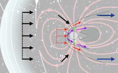
Figure 1: Schematic of both “magnetized” and “unmagnetized” cases superimposed with the same sized planet for comparison. [Adapted into a composite from Dubinin et al (2011) and public domain graphic by A. Krasse (NASA Goddard)]. Stellar wind is incoming from the left. For the ”magnetized” planet case, focus on the thick black, pink, and blue lines and arrows and ignore the thin lines: the thick pink lines are the magnetic field of the planet; the thick black arrows indicate incoming solar wind flow; the thick blue arrows indicate the outgoing flow from the atmosphere, so colored to indicate that they may also include solar wind material. The projected cross section of the magnetopause/interaction ($\sim\pi r_{s}^{2}$, where $r_{s}$ is defined in Eq. 1) is indicated by the thick vertical dotted black line at the left. The outer bubble is the bow shock and the white lines are the interplanetary field. For the ”unmagnetized” case, focus on the thin lines and arrows and ignore the aforementioned thick lines: the thin curved dotted line is the bow shock; the inner dotted line is the boundary of the induced magnetopause and the thin solid line between those two bounds the the region where pickup ions interact with the incoming flow. The red arrows indicate the incoming flow and the violet arrows indicate the pickup ion flow swept by the stellar wind. The green distance between the ionopause and the bow shock can be of order a gyro-radius away of thermal ions, and increases away from the dayside ionopause as the flux pile up decreases and the field weakens to its ambient value. The projected cross section of the magnetopause/interaction area for this ”unmagnetized” case ($\sim\pi r_{T}^{2}$, see Eq. 2), is indicated by the dotted vertical red line.

The rate of stellar wind ions entering a planet’s atmosphere depends on the product of the effective area onto which ions are captured and the speed of the inflow. We focus on comparing planets of two extremes which we delineate as “magnetized” and “unmagnetized”. The difference is shown schematically in Figure 1, where the two cases are superimposed. For present purposes, “magnetized” planets are those for which the standoff distance is determined by a magnetopause of radius $r_{s}>>r_{p}$. The thick lines of Fig. 1 correspond to this case; the incoming flow is represented by the black lines and the outgoing mixture of wind and atmosphere flow is given by thick blue lines. The cross section for interaction is given by the dotted black line. an Complementarily, our “unmagnetized” case refers to planets whose standoff distance $d_{s}$ from the incoming wind ram pressure equals the radius $r_{i}$ set by ionospheric plus induced magnetic pressure. The cross section of interaction between the stellar wind and the atmosphere is, however, determined by an interaction radius $r_{T}\geq r_{i}$ which we write as

$$r_{T}=r_{i}+r_{g}$$ (2)

where $r_{g}$ is the gyro-radius of the atmospheric ions, an upper limit of which is that for the uncompressed wind magnetic field at the planet. The thin lines of Fig. 1 capture this schematically. The incoming wind flow arrows are red and the mix of wind and outgoing atmospheric ion flow arrows are purple. The green represents $r_{g}$ at the terminator such that the cross section of interaction is given by the red dotted line. For Mars and Venus, the ionopause and magnetopause (i.e., the induced magnetopause boundary) are just a few hundred km above the surface, and not dramatically delocalized from the exobase radius (Russell, Luhmann & Strangeway, 2016). For oxygen ions, $r_{g}$ can be comparable to, or even significantly larger than the planet radius (particularly for Mars) as we discuss further in section 4.2.2. For a more compact case, it is possible that $(r_{i}+r_{g})-r_{p}<r_{p}$ such that $r_{T}\sim r_{p}$. This does not preclude the planet from still having a non-trivial atmosphere.

For our “unmagnetized” case then, the incoming mass per unit time potentially influencing the cross section determined by $r_{T}$ is given by

$${\dot{M}}_{c}\simeq\frac{\pi r_{T}^{2}}{4\pi R^{2}}{{\dot{M}}_{w}},$$ (3)

where ${\dot{M}}_{w}$ is the star’s mass loss rate per unit time of the wind, and $R$ is the planet-star distance.

In contrast, for the “magnetized” case, we consider particle capture by the magnetosphere to occur primarily during reconnection events between the stellar wind is fand the planetary magnetosphere. This is because we are considering the magnetized case to have a magnetopause so far from the exobase that the atmospheric density is too low for interacting in that region to cause significant atmospheric mass loss. The reconnection allows the wind plasma closer access to the atmosphere. Other pathways to particle capture such as Kelvin-Helmholtz mixing or impulsive penetration can also occur (Gunell et al., 2012), but we focus on magnetic reconnection as the primary facilitator.

Paschmann, Oieroset & Phan (2013) point out that about 50% of the time reconnection is favorable at the Earth’s magnetopause. This is not directly attributable to the fact that after averaging over many rotations and cycle periods over which the field periodically reverses, the shear angle between the wind field and magnetospheric field would be favorable to reconnection approximately half of the time. Rather, the favorability depends on a combination of shear angle, current sheet thickness, and variation in the plasma $\beta$ (ratio of plasma to magnetic pressure) across the magnetopause. Reconnection is still possible with small shear angles (and thus strong guide field) but requires more symmetry in $\beta$ across the magnetopause interface than the large shear angle cases. In this respect, there need not be a strict correlation between mass loading and field orientation of the solar wind.

During the reconnection phase, the effective mass capture area for stellar wind ions can approach the magnetopause cross section (on the dayside). Determining the overall efficacy of the magnetosphere at keeping incident wind particles out then requires accounting for the competing effects of the increased collection area with the reduced speed. With this in mind, the mass collected per unit time ${\dot{M}}_{c,m}$ is given by

$${\dot{M}}_{c,m}=\frac{\pi r_{s}^{2}}{4\pi R^{2}}\frac{v_{in}}{v_{w}}{{\dot{M}}_{w}\over 2},$$ (4)

where $v_{in}$ is the effective inflow speed, taken to be the reconnection speed $v_{rec}$ derived below. The factor of ${{\dot{M}}_{w}\over 2}$ accounts for the fact that the incoming wind loads into the atmosphere only when there is reconnection.

The ratio of the mass per unit time captured by a planet with a magnetosphere to that captured by the same planet without a magnetosphere is given by the ratio of Eq. (4) to Eq. (3). This is

$$Q\equiv{{\dot{M}}_{c,m}\over{\dot{M}}_{c}}={1\over 2}\left(r_{s}\over r_{T}\right)^{2}\left(v_{in}\over v_{w}\right).$$ (5)

Not all of the variables in Eq. (5) are independent, but we can simplify crudely as follows: reconnection at the standoff point is generally asymmetric across the current sheet and the incoming speed of reconnection from the wind-side toward the sheet is given by (Cassak & Shay, 2007)

$$\begin{array}[]{r}v_{in}=v_{rec}\sim 2{\tilde{\chi}}\left({B_{w}B_{2}^{3}\over 4\pi(B_{w}+B_{2})(B_{w}\rho_{2}+B_{2}\rho_{w})}\right)^{1/2},\end{array}$$ (6)

where $B_{w}$ is the field on the wind-side of the magnetopause, $B_{2}$ is the planet field on the magnetospheric side of the reconnection region, and ${\tilde{\chi}}$ is the ratio of current sheet thickness to length. For Earth at least, data suggest $B_{2}>B_{w}$ and $B_{2}\rho_{w}>B_{1}\rho_{2}$ (Sonnerup et al., 2016) so $v_{in}$ reduces to

$$\begin{array}[]{r}v_{in}=v_{rec}\sim{2B_{w}^{1/2}B_{2}^{1/2}\over(4\pi\rho_{w})^{1/2}}{\tilde{\chi}}\simeq\chi\left({B_{p}\over\sqrt{4\pi\rho_{w}}}\right)\left({r_{p}\over r_{s}}\right)^{3},\end{array}$$ (7)

where $\chi=2{\tilde{\chi}}\sqrt{B_{w}/B_{2}}$, and we use the dipole scaling $B_{2}=B_{p}({r_{p}/r_{s}})^{3}$ where $B_{p}$ is the surface field strength. Observations and simulations are roughly consistent with $\tilde{\chi}=0.1$ (Cassak & Shay, 2007) and in turn $0.5\geq\chi\geq 0.1$.

We now combine Eqs. (7) and (1) with Eq. (5) for the specific case in which $r_{T}\sim r_{p}$, the unmagnetized case with a compact atmosphere. The result is

$$v_{in}/v_{w}={\chi}{\sqrt{2}},$$ (8)

and

$$Q={\chi\over\sqrt{2}}(r_{s}^{2}/r_{p}^{2})=7.07\left({\chi\over 0.1}\right)\left({r_{s}/r_{p}\over 10}\right)^{2},$$ (9)

where we have scaled to present day Earth-like values of $\chi$ and $r_{s}/r_{p}$. That $Q$ can exceed unity highlights the important effect of the increased collecting area that the magnetosphere provides. Eq. (9) shows that the weaker the wind, the higher the rate of mass capture for a magnetized planet relative to an unmagnetized planet since $r_{s}/r_{p}$ increases for weaker stellar winds. In what follows, we assume $\chi$ to be relatively constant over the range of $r_{s}/r_{p}$ calculated. This is consistent with our assumption that the current sheet geometry is relatively constant and the fact that $\xi$ depends on the ratio of $B_{w}$ to $B_{2}$. Both of these two field strengths are likely larger for younger stars; $B_{w}$ is correlated with the surface field which is stronger for younger stars with higher coronal thermal power for the wind. The wind’s thermal energy supplies its ram pressure which, in turn, reduces $r_{s}$ and increases $B_{2}.$.

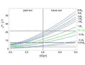
Figure 2: Standoff distance in units of Earth-like planet radius vs. age for different planet dipole moments and different wind evolution models: top (Blackman & Owen, 2016); bottom figure adapted from (Tarduno et al., 2010). Green lines of both panels represent models whose endpoint matches present day measurements. Solar wind model curves in bottom panel result from combining mass-loss to X-ray flux correlation with X-ray flux to age correlation (see text). Magnetic dipole data sources for bottom panel are as follows: Karelia (Smirnov, Tarduno & Pisakin, 2003), KVP, DP (Kaapvaal Pluton, Dalmien Pluton respectively) (Tarduno et al., 2007), and BGB, NGB (Barberton Greenstone Belt, Nondweni Greenstone Belt) (Tarduno et al., 2010). The geodynamo may have started shortly after the lunar forming event, when core chemical stratification was disrupted (e.g. Jacobson et al., 2017). In both panels: solid orange and solid black lines are thresholds of $r_{s}/r_{p}$ above which mass (Eq. (16)) and energy (Eq. (19)), respectively, per solid angle captured toward the poles are higher for a magnetized planet. Dashed orange and dashed black lines are the corresponding thresholds for total wind mass (Eq. (9)) and energy (Eq. (18)) respectively. Dashed black is absent on bottom panel due to the smaller ordinate range.

2.3 Focusing toward the polar caps

Magnetic polar caps subtend a solid angle no larger than that of a hemisphere (2$\pi$) and could be much less, as in the case of Earth. When captured particles funnel toward polar caps along the magnetic field rather than being uniformly distributed over a hemisphere, the associated local mass flux (mass per unit time per area) and energy flux within the cap solid angle is enhanced by a factor $1/f_{c}$, where

$$f_{c}=(1-cos\theta_{c})\leq 1$$ (10)

is the areal fraction of a hemisphere subtended by a polar cap of colatitude $\theta_{c}$.

If we restrict ourselves to the case when the incoming wind flow is perpendicular to the planet’s magnetic dipole axis, we can then estimate $\theta_{c}$ for a dipole from the equation for the local polar geometry of field lines, namely (Russell, Luhmann & Strangeway, 2016)

$$r{d\theta\over dr}={B_{\theta}\over B_{r}}.$$ (11)

For a vector dipole field in spherical coordinates of magnetic moment $\bf m$

$${\displaystyle\mathbf{B}({\mathbf{r}})={\frac{|\mathbf{m}|}{|\mathbf{r}|^{3}}}\left(2\cos\theta\,\mathbf{\hat{r}}+\sin\theta\,{\boldmath{\hat{\theta}}}\right)},$$ (12)

from which the ratio of the two field components is

$${B_{\theta}\over B_{r}}={tan\theta\over 2}.$$ (13)

Using Eq. (13) in Eq. (11) and integrating gives

$$r=r_{e}sin^{2}\theta,$$ (14)

where $r_{e}$ is the value of $r$ at which a particular field line crosses the equator $(\theta=\pi/2)$. The value $\theta=\theta_{c}$ is determined by setting $r_{e}=r_{s}$, the magnetopause radius, and $r=r_{p}$ because the field lines anchored on the two polar circles $\theta=\theta_{c}$ at $r=r_{p}$ represent the anchor loci of the closed field lines just at the inner edge of the magnetopause. Field lines anchored with $\theta\leq\theta_{c}$ extend into the wind-side of the magnetopause, along which wind plasma can only enter during reconnection.

Using the aforementioned substitutions in Eq. (14) along with Eq. (10) gives

$$f_{c}=1-\sqrt{1-r_{p}/r_{s}}.$$ (15)

For a fixed wind mass flux, decreasing the magnetic field increases $r_{p}/r_{s}$, thereby decreasing $f_{c}$. Correspondingly, for a fixed planetary magnetic field, $f_{c}$ decreases with increasing wind ram pressure. This implies that $f_{c}$ would generally increase with stellar age (as wind power weakens) for steady planetary field strengths.

We define $q\equiv Q/f_{c}$ as the ratio of mass capture rate per solid angle by a magnetized planet that includes polar cap channeling to that in the absence of a magnetosphere altogether. From Eq. (9) we then obtain

$$q\simeq{Q\over f_{c}}\simeq 70.7\left({{\chi}\over 0.1}\right)\left({r_{s}\over 10r_{p}}\right)^{3}\left[1+\left(1-{r_{p}\over r_{s}}\right)^{1/2}\right],$$ (16)

where the factor in square brackets ranges between 1 and 2. Note that $q/Q=1/f_{c}$, which increases with stellar youth.

Taken at face value, Eqs. (9) and (16) highlight that the mass captured by a magnetized Earth-like planet, when averaged over many wind field reversals could be greater than without a magnetic field. Our analysis here supersedes that of Tarduno, Blackman & Mamajek (2014) where we did not give explicit expressions for the reconnection speed and polar focusing or emphasize that $Q$ and $q$ can exceed unity while the analogous energy rate ratio can still be much less than unity.

2.4 Incoming energy flux with and without a magnetosphere

The ratio of energy input rates imparted to the atmosphere for magnetized vs. unmagnetized planets can be obtained by multiplying Eq. (9) and Eq. (16) by

$$\xi={\left({c_{s}^{2}\over\Gamma-1}+v_{in}^{2}\right)\over\left({c_{s}^{2}\over\Gamma-1}+v_{w}^{2}\right)}={\left({c_{s}^{2}/v_{w}^{2}\over\Gamma-1}+2{\chi}^{2}\right)\over\left({c_{s}^{2}/v_{w}^{2}\over\Gamma-1}+1\right)},$$ (17)

where $c_{s}$ is the incoming sound speed and $\Gamma$ is the adiabatic index. The energy flux includes contributions from the enthalpy and the bulk kinetic energy of the incoming material with sound speed $c_{s}$. Multiplying Eq. (9) and Eq. (16) by Eq. (17) then gives the ratios of energy capture rates of the magnetized to unmagnetized planet for unfocused and polar focused cases as

$$Q_{en}\sim 0.21\left({\xi\over 0.03}\right)\left({\chi\over 0.1}\right)\left({r_{s}/r_{p}\over 10}\right)^{2},$$ (18)

and

$$\begin{array}[]{l}q_{en}={Q_{en}\over f_{c}}\\ \simeq 2.12\left({\xi\over 0.03}\right)\left({\chi\over 0.1}\right)\left({r_{s}\over 10r_{p}}\right)^{3}\left[1+\left(1-{r_{p}\over r_{s}}\right)^{1/2}\right],\end{array}$$ (19)

respectively. The scaling of $\xi=0.03$ arises if we use fiducial values for the incoming wind of $c_{s}\simeq 3.9\times 10^{6}$cm/s (corresponding to $T\simeq 10^{5}$K), $v_{w}=400{\rm km/s}$, and $\Gamma=5/3$. Eq. (18) shows that the total energy collected by a magnetized planet scaled to present day Earth-sun-like parameters is less than that of the magnetized planet. However Eq. (19) shows that the polar energy flux concentration can be comparable, or even greater for the magnetized planet.

3 Limits on Mass Loss Rates from Energy and Momentum Conservation

The exact determination of the induced mass loss from an incoming stellar wind depends upon detailed plasma and chemical properties that determine how the incoming energy and momentum is converted to outgoing particles (Sibeck et al., 1999; Lammer, 2013; Russell, Luhmann & Strangeway, 2016). We re-emphasize here that we are considering atmospheric mass loss estimates that involve the wind and not those arising only from radiative forcing. The latter is needed to produce ions, but atmospheric mass loss direct from only radiation without the influence of the stellar wind is insufficient to explain the full history of mass loss for Earth and Venus, and even Mars (Dubinin et al., 2011; Dong et al., 2018b).

The extent to which an intrinsic planetary field can trap outgoing particles can also limit the otherwise induced loss. But regardless of how the energy and momentum inputs are subsequently converted into outgoing particles, we can compare estimates of approximate maximum atmospheric mass loss rates (“approximate” is explained below) that the wind could induce for magnetized and unmagnetized cases. The distinction between these two cases is essential when the exobase is below the magnetopause or ionopause.

The wind energy flux times the capture area for inflow speed $v_{in}$ is given by

$$\rho_{in}Av_{in}\left({c_{s}^{2}\over\Gamma-1}+v_{in}^{2}\right)={\dot{M}}_{in}\left({c_{s}^{2}\over\Gamma-1}+v_{in}^{2}\right),$$ (20)

and the wind momentum flux times the capture area is

$$\rho_{in}A\left(v_{in}^{2}+{c_{s}^{2}\over\Gamma}\right)={\dot{M}}_{in}v_{in}\left(1+{c_{s}^{2}\over\Gamma v_{in}^{2}}\right).$$ (21)

The maximum outflow induced mass loss rate corresponds to the case in which all of the incoming momentum or energy gets converted into outflow with outflowing ions moving just at the escape speed $v_{esc}$ along open field lines. For thermal, isotropically distributed ions, the relevant initial ion speed would be the most probable particle speed at the exobase $v_{p}$. If $v_{p}$ were already even as high as a fraction $\lambda=1/4$ of the escape speed $v_{esc}$ before any wind influence, then for a Maxwellian distribution $f(v)=({-mv^{2}\over 2\pi kT})^{3/2}e^{-mv^{2}\over 2kT}$, only a fraction ${\int_{v_{p}/\lambda}^{\infty}f(v)v^{2}dv\over\int_{0}^{\infty}f(v)v^{2}dv}\sim 7.4\times 10^{-9}$ would be above the escape speed, and the fraction drops exponentially with decreasing $\beta$. When this fraction times the atmospheric density at the exobase is less than that of the stellar wind, the number of particles above the escape speed would be negligible.

But even particles with speeds as high as $v_{esc}/4$, have only 1/16th of the escape energy. Therefore, assuming that particles start from zero energy does not lead to a significant difference in estimating a mass loss rate. Moreover, for cases when the particle gyro-radii are initially much smaller than the planet scale, then only motion along open field lines leads to escape. Since the escape path is locally along 1 direction, no more than 1/3 of the particles escape when the most probable speed reaches the escape speed for an isotropic distribution. To ensure that all particles escape if they were initially at $1/16$ the escape energy then requires $3-1/16\sim 3$ times the escape energy to be imparted from the incoming wind.

If the ratio of the inflow speed to the escape speed exceeds unity, then energy conservation gives a larger outflow mass loss rate limit than momentum conservation. Otherwise, momentum conservation determines the larger mass loss rate limit. For a steady state, the corresponding energy and momentum rate balance equations for inflow and outflow are given respectively by

$${\dot{M}}_{in}\left({c_{s}^{2}\over\Gamma-1}+v_{in}^{2}\right)={\dot{M}}_{out}v_{esc}^{2},$$ (22)

and

$${\dot{M}}_{in}v_{in}\left(1+{c_{s}^{2}\over\Gamma v_{in}^{2}}\right)={\dot{M}}_{out}v_{esc}.$$ (23)

By rearranging each of Eq. (22) and (23) to obtain an expression for ${\dot{M}}_{out}$, we can combine the results to express the maximum of the two upper limit estimates for the outflow mass loss. If we also allow for the polar focusing fraction $f_{c}$, the combined result is

$$\begin{array}[]{l}{{\dot{M}}_{out,max}\over{{\dot{M}}_{in}}}\\ ={1\over f_{c}}{v_{in}\over v_{esc}}\left[{{v_{in}\over v_{esc}}\left(1+{c_{s}^{2}/v_{in}^{2}\over\Gamma-1}\right)},\left(1+{c_{s}^{2}/v_{in}^{2}\over\Gamma}\right)\right],\end{array}$$ (24)

where the first term in brackets is the result from energy conservation and the second term is from momentum conservation. The former dominates when $v_{in}>v_{esc}$, and the latter when $v_{in}<v_{esc}$. If all the energy and momentum instead went into particles moving at some speed $v_{ave}>v_{esc}$, then $v_{ave}$ would replace $v_{esc}$ in Eq. (24) and the mass outflow rate estimate would be correspondingly reduced.

4 Implications for Atmosphere Protection

We now apply the formalism of the previous sections to the time evolution of magnetospheric protection for the Earth-sun system, and to the separate question of present day oxygen ion loss rates from Earth, Mars, and Venus.

4.1 Influence of stellar activity variation on protection by an Earth-like magnetosphere

The blue curves of the top panel and the red curves of the bottom panel of Fig. 2 show the time evolution of $r_{s}/r_{p}$ for different values of the planetary magnetic field (assumed to be constant for each curve) for an Earth-like planet at 1AU from a sun-like star. The top panel uses the minimalist, but holistic theoretical model of (Blackman & Owen, 2016) to compute the standoff distance from the wind ram pressure. The latter is derived from the time evolution of magnetic field, rotation, mass loss, and X-ray luminosity predicted from the physics of the model. Although the correlation between X-ray luminosity and stellar mass loss has been questioned (Cohen, 2011), this query is based on short-term observations of the Sun that may not apply to the billion year time scales of interest. The bottom panel in Fig. 2 shows curves from Tarduno et al. (2010) which utilize the empirical mass loss values for solar-like stars from (Wood, 2006) based on H I Lyman-$\alpha$ data. Those values are observed to correlate with X-ray flux, which in turn was used to empirically determine stellar ages. The magnetopause standoff distances are truncated at 700 my because the few available young stellar analogs hint at lower rates of mass loss (Wood et al., 2014), breaking the correlation. (The saturation of X-ray flux with youth also makes age determination more difficult for younger stars (Mamajek & Hillenbrand, 2008; Wright et al., 2011).)

The green curve in the top panel of Fig. 2 corresponds to the case that matches present day field measurements, as also labeled on the bottom panel. The curves of both panels show that $r_{s}/r_{p}$ decreases with youth because of the stronger ram pressure of the solar wind, while the planetary field remains nearly constant. The horizontal lines in the two panels of Fig 2 correspond to the specific thresholds calculated in Section 2. Namely, the orange solid lines show the threshold of $r_{s}/r_{p}$ above which $q\geq 1$ from Eq. (16) (assuming the lower limit of $1$ for the square bracketed quantity). The orange dashed lines show the threshold above which $Q\geq 1$ from Eq. (9). These are, respectively, the thresholds above which the polar and total atmospheric mass collection rates for the magnetized planet exceed those for the unmagnetized planet with a compact atmosphere. The solid and dashed black curves, which correspond to Eqs (19) with the square bracketed quantity equal to $1$, and (18) respectively, indicate the threshold ratio of $r_{s}/r_{p}$ above which the polar focused and total energy capture rates by the magnetized planet exceed that for an unmagnetized planet. Because energy conservation rather than momentum conservation determines the larger of the two values on the right of Eq. (24) for Earth-sun-like systems, these curves also indicate the corresponding thresholds above which the magnetized planet has higher upper limits on mass loss from stellar-wind atmosphere erosion as compared to the unmagnetized planet.

Given the fiducial parameter values used to make the horizontal lines, both panels of Fig. 2 reinforce the same implications: for most of an Earth-like planet’s history, more total mass and polar mass flux can be captured by the magnetized planet than for the correspondingly unmagnetized planet, even though less total energy is captured by the magnetized planet over its past history. As shown, this circumstance will also persist for the the long term future. Since the maximum mass outflow rate for an Earth-sun-like system is determined by energy rather than momentum in Eqn. (24), this further implies that the upper limit on the mass loss rate would be reduced by a magnetosphere throughout the Earth-like planet’s past and future.

If we include polar focusing using $f_{c}$ from Eq. (10) however, the solid black horizontal lines of Fig 2 exemplify that the polar focused energy flux (and thus the resulting upper limit on atmospheric mass outflow from Eq. (24)) can be higher in the recent past and future for the magnetized Earth compared to an unmagnetized Earth. Here the two panels differ somewhat in where the line crosses the standoff curve that best matches present day but as alluded to above, neither the data nor the models are accurate enough for this time scale to be constrained to better than a factor of 2.

Irrespective of the cross-over time discussed above, Fig. 2 shows, for an Earth-like magnetized planet, that the initial outgoing mass loss due to interaction with the wind (and ignoring return flow) can be larger with a magnetosphere than without under certain conditions because the magnetosphere can capture and focus more incoming wind energy than would otherwise have access to the atmosphere. How close the actual mass loss corresponds to the maximum limit implied by Eq. (24) depends on rate of ion return and on how incoming energy and momentum interact with specific planetary atmospheres. We touch on the latter in the next section.

4.2 Partial explanation of Oxygen ion loss from Mars, Venus, and Earth

The question of why $O^{+},O^{+}_{2}$ loss rates on Earth, Mars and Venus are apparently within a few orders of magnitude of each other is of interest. This has led some to question the traditionally assumed protective role of an internally generated magnetosphere (Strangeway et al., 2010; Wei et al., 2012; Strangeway et al., 2017) since Earth has one but Mars and Venus do not. The detailed processes and local conditions of different atmospheres are time dependent, and the measured rates depend on solar activity phase and spacecraft location, so there is a range of more than an order of magnitude even for a given planet. The complexity of the underlying systems ultimately require combining the chemistry and microphysics to obtain detailed models. The diversity of numerical simulations of this sort include M-star stellar winds interacting with habitable magnetized, and Venus-like planets, to obtain standoff distances and lower limits on mass loss (Cohen et al., 2014, 2015); studies of the Trappist exoplanet system (Dong et al., 2018a); and simulations of the time evolution of Mars’ oxygen loss (Dong et al., 2018b) that presently agrees with recent MAVEN data (Jakosky et al., 2015).

We will use our formalism to obtain approximate upper limits on oxygen ion escape rates for Earth, Mars, and Venus-like planets from interaction with the solar wind, using energy and momentum conservation separately. We will compare the results for internally magnetized (Earth-like) and non-internally magnetized (Mars and Venus-like) cases. Zendejas, Segura & Raga (2010), presented a different minimalist model of ion outflow rates, using an imposed efficiency parameter $\alpha$ to characterize how much inflow energy is converted to outflow. A value $\alpha=1$ would make their results also upper limits, but they do not address the case of a magnetized planet.

We will see that the atmospheric mass loss estimates that result from use of momentum conservation in our approach are in fact similar for Earth, Venus, and Mars to the level of an order of magnitude. Our limits that result from use of energy conservation are similar for the three planets to within two orders of magnitude.

4.2.1 Upper Limits for Earth

To obtain an atmospheric mass loss limit ${\dot{M}}_{out}\leq{\dot{M}}_{out\oplus}$ for an Earth-like magnetized planet, we consider the fluxes as integrated over solid angle and thus avoid $f_{p}$ here. We then use Eq. (8), Eq. (4), and energy conservation in Eq. (24) to obtain

$$\begin{array}[]{l}{\dot{M}}_{out\oplus}=7\times 10^{4}\left({\dot{M}_{w}\over 1.3\times 10^{12}{\rm g/s}}\right)\left({v_{w}\over 4\times 10^{7}{\rm cm/s}}\right)^{2}\left({\chi\over 0.1}\right)^{3}\\ \left({r_{s}\over 10r_{\oplus}}\right)^{2}\left({R\over 1{\rm AU}}\right)^{-2}\left({r_{ex}\over 1.2r_{\oplus}}\right)\left({M_{p}\over M_{e}}\right)^{-1}\left({{{c_{s}^{2}/[2\chi^{2}v_{w}^{2}(\Gamma-1)]}+1}\over 1.64}\right){\rm g\over s}.\end{array}$$ (25)

If instead we use momentum conservation in Eq. (24), we obtain

$$\begin{array}[]{l}{\dot{M}}_{out\oplus}=1.5\times 10^{4}\left({\dot{M}_{w}\over 1.3\times 10^{12}{\rm g/s}}\right)\left({v_{w}\over 4\times 10^{7}{\rm cm/s}}\right)\left({\chi\over 0.1}\right)^{2}\\ \left({r_{s}\over 10r_{\oplus}}\right)^{2}\left({R\over 1{\rm AU}}\right)^{-2}\left({r_{ex}\over 1.2r_{\oplus}}\right)^{1\over 2}\left({M_{p}\over M_{e}}\right)^{-{1\over 2}}\left({{{c_{s}^{2}/(2\chi^{2}v_{w}^{2}\Gamma)]}+1}\over 1.26}\right){\rm g\over s},\end{array}$$ (26)

where $M_{p}$ is the planet mass, $r_{ex}$ is the exobase radius, which, along with $r_{s}$ are scaled to Earth’s radius $r_{\oplus}$. For Earth, $r_{ex}\sim 1.2r_{\oplus}$ and $r_{s}\sim 10r_{\oplus}$, ${\chi}=0.1$. From Eq. (24), the corresponding particle loss rates limits from Eq. (25) and Eq. (26) are respectively

$$dn/dt\leq{{\dot{M}}_{out\oplus}\over\mu m_{p}}\simeq 2.62\times 10^{27}\left({\mu\over 16}\right)^{-1}{\rm s}^{-1},$$ (27)

and

$$dn/dt\leq{{\dot{M}}_{out\oplus}\over\mu m_{p}}\simeq 5.6\times 10^{26}\left({\mu\over 16}\right)^{-1}{\rm s}^{-1}.$$ (28)

This can be compared with $7.2\times 10^{25}$/s of $O^{+}$ observed with speeds above escape leaving the poles, and averaged over a solar cycle, of which 90% seems to be recaptured (Seki et al., 2001).

4.2.2 Upper Limits for Venus and Mars

For Mars and Venus, photoionization and dissociative recombination convert neutral molecules into $(O^{+}$ or $O_{2}^{+})$ and these collisionless ions can then be accelerated by the motional electromotive force (Lundin & Dubinin, 1992; Dubinin et al., 2011; Russell, Luhmann & Strangeway, 2016) near the ionopause. These ions then drift perpendicular to both the incoming wind velocity and magnetic field. Since the incoming flow has no initial net momentum perpendicular to the flow, lateral acceleration of oxygen ions is accompanied by a momentum conserving flow in the opposite direction. Electrons can play this role when ion-gyro-radii are small, but in a multi-ion-species plasma with gyro-radii comparable or larger than system scales, proton streaming in the opposite direction to the oxygen atoms is also important (Dubinin et al., 2011).

As oxygen atoms drift away from the subsolar point, their Larmor orbits take them into the wind plasma where they are picked up by the oncoming wind, accelerated and carried past the planet. For Venus, the ion production mechanisms likely do not directly accelerate ions to escape speeds so the wind-atmosphere interaction is essential but for Mars the initial energy of the ions from dissociative recombination might produce some escape ions directly. Photochemical dissociation may dominate presently, but ion-pickup could dominate for ancient Mars (Dong et al., 2018b). As discussed in section 3, even if the ions initially have speeds as high as 1/4 the escape speed before acquiring wind energy, the requirements to escape would be nearly the same as if particles started from zero energy.

Focusing first on Venus, we note that standoff is determined by the ionopause particle pressure, but the induced magnetic field piles up just outside this region to a value in near equipartition with the internal thermal pressure (Russell, Luhmann & Strangeway, 2016). The induced magnetopause boundary is of order $50$ km or so above the ionopause, and the latter is only $\sim 250$ km above the surface. Since the ionopause, magnetopause, and exobase are all only within a few $100$ km above the surface, they are relatively small distances above the planet radius $r_{p}$. However, the influence of the wind on atmospheric mass loss requires coupling of the wind and ionosphere. Once the ions are picked up by the wind, this coupling is determined by finite gyro-radii–an estimate of which will be needed to determine $r_{T}$ in the cross section for interaction between wind and atmosphere.

To quantify the atmospheric mass loss, we first apply Eq. (3) for ${\dot{M}}_{in}$ in combination with Eq. (24) and $v_{in}=v_{w}$ to obtain ${\dot{M}}_{out}\leq{\dot{M}}_{out\venus}$. Using energy conservation in Eq. (24), we obtain

$$\begin{array}[]{l}{\dot{M}}_{out\venus}={1.5\times 10^{6}}\left({\dot{M}_{w}\over 1.3\times 10^{12}{\rm g/s}}\right)\left({v_{w}\over 4\times 10^{7}{\rm cm/s}}\right)^{2}\left({R\over 0.72{\rm AU}}\right)^{-2}\\ \left({\pi r_{T}^{2}\over 8\times 10^{18}{\rm cm^{2}}}\right)\left({r_{ex}\over 0.95r_{\oplus}}\right)\left({M_{p}\over 0.81M_{e}}\right)^{-1}\left({{{c_{s}^{2}/[v_{w}^{2}(\Gamma-1)]}+1}\over 1.01}\right){\rm g/s}.\end{array}$$ (29)

If instead we use momentum conservation in Eq. (24), we obtain

$$\begin{array}[]{l}{\dot{M}}_{out\venus}=3.86\times 10^{4}\left({\dot{M}_{w}\over 1.3\times 10^{12}{\rm g/s}}\right)\left({v_{w}\over 4\times 10^{7}{\rm cm/s}}\right)\left({R\over 0.72{\rm AU}}\right)^{-2}\\ \left({\pi r_{T}^{2}\over 8\times 10^{18}{\rm cm^{2}}}\right)\left({r_{ex}\over 0.95r_{\oplus}}\right)^{1/2}\left({M_{p}\over 0.81M_{e}}\right)^{-1/2}\left({{{c_{s}^{2}/(v_{w}^{2}\Gamma)}+1}\over 1.00}\right){\rm g/s},\end{array}$$ (30)

where in both Eq. (29) and (30) we have used $r_{T}$ as defined in Eq. (2) with $r_{g}$ computed for $O^{+}$ ions at the solar wind speed using a Parker spiral field (Parker, 1958) estimate for the uncompressed wind magnetic field $B(R)=B_{\odot}(R_{\odot}^{2}/R)(\Omega_{\odot}/v_{w})$ at Venus’ distance from the sun. This provides a maximum estimate for $r_{g}$ since a larger field and smaller thermal speed lowers $r_{g}$. The result is

$$r_{g}=9.9\times 10^{8}{\rm cm}\left({\mu\over 16}\right)\left({v_{w}\over 4\times 10^{7}{\rm cm/s}}\right)\left({B\over 7\times 10^{-5}{\rm G}}\right)^{-1}.$$ (31)

For $\mu=16$, the corresponding ion loss rates are then

$$dn/dt\leq{{\dot{M}}_{out\venus}\over\mu m_{p}}\simeq 5.58\times 10^{28}{\rm s}^{-1}$$ (32)

and

$$dn/dt\leq{{\dot{M}}_{out\venus}\over\mu m_{p}}\simeq 1.44\times 10^{27}{\rm s}^{-1}.$$ (33)

This latter limit is an order of magnitude larger than the highest values reported in (Knudsen & Miller, 1992; Dubinin et al., 2011) for ions above the escape energy.

For Mars, aside from its localized magnetic features, much of the surface has too little magnetic or ionospheric pressure to steadily abate the incoming wind ram pressure (Russell, Luhmann & Strangeway, 2016). We again use Eq. (29) but now with the Martian parameters of $M_{p}=0.11M_{e}$; $r_{p}\sim r_{s}=r_{ex}=0.53r_{\oplus}$, and $R=1.5AU$ in Eqn. (24). For $r_{T}$ we use Eq. (2) but employing Mars’ radius for $r_{p}$ and $r_{g}$ is now the gyro-radius for $O_{2}^{+}$ ions moving at the solar wind speed in the uncompressed solar wind field at Mars, namely, $r_{g}=4.2\times 10^{9}\left({\mu\over 32}\right)\left({v_{w}\over 4\times 10^{7}{\rm cm/s}}\right)\left({B\over 3.3\times 10^{-5}{\rm G}}\right)^{-1}{\rm cm}$.

The resulting mass loss limit from energy conservation from Eq. (24) is then ${\dot{M}}_{out\mars}=1.3\times 10^{5}$g/s and for $\mu=32$, the corresponding ion loss rate is then

$$dn/dt\leq{{\dot{M}}_{out\mars}\over\mu m_{p}}\simeq 2.3\times 10^{29}{\rm s}^{-1}.$$ (34)

If instead we use momentum conservation in Eq. (24), then we obtain ${\dot{M}}_{out\mars}=1.6\times 10^{3}$g/s and the corresponding ion loss rate limit of

$$dn/dt\leq{{\dot{M}}_{out\mars}\over\mu m_{p}}\simeq 2.9\times 10^{27}{\rm s}^{-1}.$$ (35)

These can be compared with values up to $2\times 10^{25}/{\rm s}$ at solar max reported in Dubinin et al. (2011).

Comparing the results from Eqs. (27) & (28); (32) & (33); and and (34) & (35) we see that (i) the wind-induced mass loss limit estimates from energy conservation span 2 orders of magnitude with ${\dot{M}}_{out\mars}>{\dot{M}}_{out\venus}>{\dot{M}}_{out\oplus}$, and all exceed the respective limits from momentum conservation for each of the three cases; (ii) the mass loss limits from momentum conservation satisfy the same inequality ordering but all are within an order of magnitude of each other; (iii) the momentum limits are all appropriately larger than the largest measured values. It is a worthy pursuit to identify the basic principles that dictate how efficiently the incoming energy and momentum are redistributed among particles and on what this depends. Momentum limits may be more pertinent than energy limits for unmagnetized planets as the flow has more direct access to the atmosphere. In addition, we might speculate that the maximum efficiency with which momentum is converted to oxygen ions given the aforementioned comparisons of predicted versus measured values is of the order of 10% for Earth and Venus and 1% for Mars. The latter is perhaps consistent with the possibility emerging from at least one global model, namely that photodissociation may dominate Mars’ present ion loss, but that of ancient Mars ($\sim 4$ Ga) was two orders of magnitude larger, and dominated by ion-pickup (Dong et al., 2018b). That said, the relative role of photodissociation vs. ion-pickup is still an area of active study. However, given the current limitations on observed loss rates and incoming wind flux, these pursuits are left for future study.

In short, our formalism may help to explain aspects of the present-day loss rates of terrestrial planets with atmospheres. We reiterate that this is separate from the specific question of the role of magnetic fields in sustaining or inhibiting habitability. The present state of Venus and Mars reflects a longterm atmospheric evolution with a profound loss of the principal component defining habitability–water. Present day Venus is particularly inhabitable. As such, the present-day atmospheric erosion rates do not provide direct measures of depletion of a specifically habitable atmospheres but still offer testbeds for basic principles of atmospheric mass loss given different sources of external stellar forcing. Those principles are still important to identify even if they do not comprise a complete set of ingredients that determine habitability.

5 Conclusions

We have considered how a planetary magnetosphere influences the upper limit on stellar wind induced mass loss by focusing on how the magnetic field affects incoming flow of mass and energy into the atmosphere. The approximate maximum outflow rates are estimated separately for the constraint of energy conservation and momentum conservation assuming that (i) all of the incoming energy or momentum goes into outgoing particles just at the escape speed; and (ii) that the atmospheres have initially thermal energy distributions with most probable speeds initially less than 1/4 the escape speed. Our formalism can be used to obtain upper limit estimates for a given planetary magnetic field, planet size, mass, orbital radius and stellar wind parameters. For the parameter regimes considered, momentum conservation provides a lower upper limit than energy conservation.

The formalism may be helpful toward a better understanding of the role and extent that magnetic fields play in protecting atmospheres of both solar system and extrasolar planets. In particular, we find that the competing effects of decreased solar wind flux interacting with the atmosphere versus increased solar wind collection area predict that (i) for most of Earth’s history, more total solar wind mass may have been captured with potential to interact with the atmosphere than would have been the case without a geodynamo but that (ii) the geomagnetic field still had a net protective from the solar wind because less wind energy was input as compared to would be the case of an unmagnetized Earth. However, when polar focusing is taken into account, the future polar energy flux collected by Earth’s magnetosphere could exceed that which would be collected without a field. The latter implies that the future protective effect of the geomagnetic field will depend primarily on its ability to recapture (Seki et al., 2001) otherwise ablated plasma. We also showed how the competing effects of decreased solar wind flux interacting with the atmosphere versus increased solar wind collection area might contribute to explaining the explain present-day oxygen ion ejection rates from Earth, Mars, and Venus.

Since the retention of water, and therefore oxygen, is a key ingredient for Earth-like habitability, our results highlight that the influence of planetary magnetic fields on the survival of habitable atmospheres must ultimately depend on the relative interplay between incoming wind flux reduction, increase wind capture area, and outgoing atmosphere re-capture.

References

- Barabash (2010) Barabash S., 2010, Geophysical Research Abstracts, EGU2010-5308
- Blackman & Owen (2016) Blackman E. G., Owen J. E., 2016, MNRAS, 458, 1548
- Brain et al. (2013) Brain D., Leblanc F., Luhmann J., Moore T., Tian F., 2013, Planetary Magnetic Fields and Climate Evolution, Mackwell S. J., Simon-Miller A. A., Harder J. W., Bullock M. A., eds., Space Science Series, Univ. of Arizona Press, Tucson AZ, pp. 487–501
- Cassak & Shay (2007) Cassak P. A., Shay M. A., 2007, Physics of Plasmas, 14, 102114
- Cohen (2011) Cohen O., 2011, MNRAS, 417, 2592
- Cohen et al. (2014) Cohen O., Drake J. J., Glocer A., Garraffo C., Poppenhaeger K., Bell J. M., Ridley A. J., Gombosi T. I., 2014, ApJ, 790, 57
- Cohen et al. (2015) Cohen O., Ma Y., Drake J. J., Glocer A., Garraffo C., Bell J. M., Gombosi T. I., 2015, ApJ, 806, 41
- Cowley & Lewis (1990) Cowley S. W. H., Lewis Z. V., 1990, Planetary and Space Science, 38, 1343
- do Nascimento et al. (2016) do Nascimento, Jr. J.-D. et al., 2016, ApJL, 820, L15
- Dong et al. (2018a) Dong C., Jin M., Lingam M., Airapetian V. S., Ma Y., van der Holst B., 2018a, Proceedings of the National Academy of Science, 115, 260
- Dong et al. (2018b) Dong C. et al., 2018b, ApJL, 859, L14
- Dubinin et al. (2011) Dubinin E., Fraenz M., Fedorov A., Lundin R., Edberg N., Duru F., Vaisberg O., 2011, Space Science Reviews, 162, 173
- Gunell et al. (2012) Gunell H. et al., 2012, Physics of Plasmas, 19, 072906
- Huang (1960) Huang S.-S., 1960, PASP, 72, 106
- Hunten (1982) Hunten D. M., 1982, Planetary and Space Science, 30, 773
- Hunten (1993) Hunten D. M., 1993, Science, 259, 915
- Jacobson et al. (2017) Jacobson S. A., Rubie D. C., Hernlund J., Morbidelli A., Nakajima M., 2017, Earth and Planetary Science Letters, 474, 375
- Jakosky et al. (2015) Jakosky B. M. et al., 2015, Space Science Reviews, 195, 3
- Karak, Kitchatinov & Choudhuri (2014) Karak B. B., Kitchatinov L. L., Choudhuri A. R., 2014, ApJL, 791, 59
- Kasting & Pollack (1983) Kasting J. F., Pollack J. B., 1983, Icarus, 53, 479
- Kasting, Whitmire & Reynolds (1993) Kasting J. F., Whitmire D. P., Reynolds R. T., 1993, Icarus, 101, 108
- Kitchatinov & Olemskoy (2015) Kitchatinov L. L., Olemskoy S. V., 2015, Research in Astronomy and Astrophysics, 15, 1801
- Knudsen & Miller (1992) Knudsen W. C., Miller K. L., 1992, JGR, 97, 17
- Kumar, Hunten & Pollack (1983) Kumar S., Hunten D. M., Pollack J. B., 1983, Icarus, 55, 369
- Lammer (2013) Lammer H., 2013, Origin and Evolution of Planetary Atmospheres. Springer, New York
- Lammer & Bauer (1991) Lammer H., Bauer S. J., 1991, JGR, 96, 1819
- Luhmann, Johnson & Zhang (1992) Luhmann J. G., Johnson R. E., Zhang M. H. G., 1992, Geophys. Res. Lett., 19, 2151
- Lundin & Dubinin (1992) Lundin R., Dubinin E. M., 1992, Advances in Space Research, 12, 255
- Lundin, Lammer & Ribas (2007) Lundin R., Lammer H., Ribas I., 2007, Space Science Reviews, 129, 245
- Mamajek & Hillenbrand (2008) Mamajek E. E., Hillenbrand L. A., 2008, ApJ, 687, 1264
- Matt et al. (2015) Matt S. P., Brun A. S., Baraffe I., Bouvier J., Chabrier G., 2015, ApJL, 799, L23
- Moore & Khazanov (2010) Moore T. E., Khazanov G. V., 2010, J. Geophys. Res., 115, A00J13
- Noyes et al. (1984) Noyes R. W., Hartmann L. W., Baliunas S. L., Duncan D. K., Vaughan A. H., 1984, ApJ, 279, 763
- Parker (1958) Parker E. N., 1958, ApJ, 128, 664