Structure-Preserving $\mathrm{\Gamma}$QR and $\mathrm{\Gamma}$-Lanczos Algorithms for Bethe-Salpeter Eigenvalue Problems

Abstract

To solve the Bethe-Salpeter eigenvalue problem with distinct sizes, two efficient methods, called $\mathrm{\Gamma}$QR algorithm and $\mathrm{\Gamma}$-Lanczos algorithm, are proposed in this paper. Both algorithms preserve the special structure of the initial matrix $\mathscr{H}=\begin{bmatrix}A&B\\ -\overline{B}&-\overline{A}\end{bmatrix}$, resulting the computed eigenvalues and the associated eigenvectors still hold the properties similar to those of $\mathscr{H}$. Theorems are given to demonstrate the validity of the proposed two algorithms in theory. Numerical results are presented to illustrate the superiorities of our methods.

1 Introduction

In this paper, we consider the following structured eigenvalue problem

$${\mathscr{H}\bm{x}}\equiv\begin{bmatrix}\hphantom{-}A&\hphantom{-}B\\ -\overline{B}&-\overline{A}\end{bmatrix}\begin{bmatrix}\bm{x}_{1}\\ \bm{x}_{2}\end{bmatrix}=\lambda\,\bm{x},$$ (1)

where $A,B\in\mathbb{C}^{n\times n}$ with $A^{H}=A,\ B^{T}=B$. Here, we denote by $A^{H}$, $\overline{A}$ and $B^{T}$, respectively, the conjugate transpose of $A$, the complex conjugate of $A$, and the transpose of $B$. Such an eigenvalue problem (1) is referred to as a Bethe-Salpeter eigenvalue problem (BSEP). Any $\lambda\in\mathbb{C}$ and nonzero $\bm{x}\in\mathbb{C}^{2n}$ that satisfy (1) are called an eigenvalue and its corresponding eigenvector of $\mathscr{H}$, respectively. Accordingly, $(\lambda,\bm{x})$ is called an eigenpair.

The BSEP (1) arises from the discretization of the Bethe-Salpeter equation effectively describing the bound states of a two-body quantum field theoretical system for the response function. Essentially, the Bethe-Salpeter equation comes from the strict derivation of the problem within Green’s-function theory, which can be used in the simulation of electron-hole interaction effects (see [1]), electron-positron interaction effects (see [2]), etc.. More details about the Bethe-Salpeter equation can be found in [3, 4, 5, 6, 7, 8, 9] and the references therein. Usually, to solve the Bethe-Salpeter equation for a finite system all equations are projected onto an orthonormal spin-orbit basis, and then we obtain its corresponding discrete form (1).

Recently, the BSEP (1) is penetratively studied under the condition that $\Gamma_{0}\mathscr{H}$ is positive definite with $\Gamma_{0}=\operatorname{diag}(I_{n},-I_{n})$ (see [10, 11, 12]). In [10], the authors firstly show that the BSEP is equivalent to a real Hamiltonian eigenvalue problem, then an efficient parallel algorithm is proposed to compute all eigenpairs corresponding to those positive eigenvalues of the equivalent real Hamiltonian matrix. By projecting the initial matrix $\mathscr{H}$ in (1) onto a reduced basis set, [11, 12] apply low-rank and QTT tensor approximation to approximate the BSEP in large-scale. After that a simplified Bethe-Salpeter eigenvalue problem, with the diagonal plus low-rank structure, is solved. Though the methods proposed in [10, 11, 12] aim to solve the BSEP, they all are principally suitable for the linear response eigenvalue problem (LREP), a special case of the BSEP. Intrinsically, the LREP requires both $A$ and $B$ are real symmetric matrices, i.e., $A^{T}=A\in\mathbb{R}^{n\times n},B^{T}=B\in\mathbb{R}^{n\times n}$. A plenty of remarkable contributions have been made to solve the LREP and please refer to [13, 14, 15, 16] and references therein for more information.

People usually use the classical QR algorithm and Lanczos method to compute all eigenvalues of a general matrix and a few number of eigenvalues and their associated eigenvectors of a Hermitian matrix, respectively. One can refer to [17, 18, 19] and the references therein to find the details of the QR algorithm and the Lanczos method. For the convergence of the Lanczos method please consult [20, 21, 22]. The classical QR algorithm can be employed to solve the BSEP in modest size, however, the special structure of $\mathscr{H}$ (see the preliminary section) will not keep any longer. Also, we use $\Pi$-tridiagonal matrices to solve the BSEP in this article, similarly to the Lanczos method. Many literatures apply the tridiagonal or quasi-diagonal matrices to solve various problems, such as boundary value Poisson equations [23, 24, 25], circulant systems [26], time series analysis [27], control theory [28] and so on.

In this paper, we will study a general BSEP and the positive definite restriction on $\Gamma_{0}\mathscr{H}$ is no longer assumed. Upon the structure-preserving $\mathrm{\Gamma}$QR algorithm proposed in [16], which solves the LREP by introducing the $\mathrm{\Gamma}$-orthogonality and performing a series of $\mathrm{\Gamma}$-orthogonal transformations to the initial $\mathscr{H}\in\mathbb{R}^{2n\times 2n}$, we put forward a similar $\mathrm{\Gamma}$QR algorithm to solve the BSEP with $\mathscr{H}\in\mathbb{C}^{2n\times 2n}$ being some dense modest size matrix. Here, $\mathrm{\Gamma}$-unitary transformations are used and some implicit multishift techniques are employed. As pointed in [10], the size of the BSEP usually can be fairly large, which actually is proportional to the number of the electrons of one system. To solve a large-scale BSEP, a $\mathrm{\Gamma}$-Lanczos  algorithm will be developed, where a decomposition analogous to the classical Lanczos decomposition is constructed. Some error bounds and a convergence theorem are given to illustrate the performance of the proposed $\mathrm{\Gamma}$-Lanczos  algorithm.

The rest of this paper is organized as follows. In Section 2, we introduce some basic definitions and give some preliminaries which will be used in subsequent sections. The $\mathrm{\Gamma}$QR  algorithm to compute the BSEP with modest size is displayed in Section 3. The $\mathrm{\Gamma}$-Lanczos  algorithm to solve the large-scale BSEP is developed in Section 4. Numerical results are presented in Section 5. Some concluding remarks are finally drawn in Section 6.

Notations

Throughout this paper, we denote the $j$-th column of the identity matrix $I$ by $\bm{e}_{j}$, whose size is determined from the context. The MATLAB expression, which specifies the submatrix with the colon notation, will be used when necessary, that is, $M(k:l,s:t)$ refers to the submatrix of $M$ formed by rows $k$ to $l$ and columns $s$ to $t$. For matrices $M$ and $N$, $\operatorname{diag}(M,N)$ represents the matrix $\begin{bmatrix}M&\\ &N\end{bmatrix}$. Additional, denote $\Pi_{2k}=\begin{bmatrix}\bf 0&I_{k}\\ I_{k}&\bf 0\end{bmatrix}$ for all positive integer $k$, and $\Pi\equiv\Pi_{2n}$ for short, where $2n$ is the size of the matrix $\mathscr{H}$.

2 Definitions and Preliminaries

Some definitions and preliminaries are presented in this section, where many definitions and propositions are quoted from [16], most of which can be trivially extended to the complex matrix $\mathscr{H}$.

Definition 2.1

Let $G\in\mathbb{C}^{2n\times 2m}$, where $m\leq n$. $G$ is a $\Pi^{\pm}$-matrix if $G\Pi_{2m}=\pm\Pi_{2n}\overline{G}$, that is, $G$ is of the form

$$G=\begin{bmatrix}\hphantom{-}G_{1}&\hphantom{-}G_{2}\\ \pm\overline{G}_{2}&\pm\overline{G}_{1}\end{bmatrix}\quad\text{ with }\quad G_{1},\ G_{2}\in\mathbb{C}^{n\times m}.$$ (2)

Denote by $\bm{\Pi}_{2n\times 2m}^{\pm}$ the set of all $2n\times 2m$ $\Pi^{\pm}$-matrices. When $m=n$, we simply write $\bm{\Pi}_{2n}^{\pm}$ for $\bm{\Pi}_{2n\times 2n}^{\pm}$.

Definition 2.2

Let $G\in\bm{\Pi}_{2n}^{\pm}$ as in (2) and set

$$G_{1i}=G_{1}(1:i,1:i),\quad G_{2i}=G_{2}(1:i,1:i).$$

$\begin{bmatrix}G_{1i}&G_{2i}\\ \pm\overline{G}_{2i}&\pm\overline{G}_{1i}\end{bmatrix}$ is called the $i$-th $\Pi^{\pm}$-leading principal submatrix of $G$ and its determinant is called the $i$-th $\Pi^{\pm}$-leading principal minor of $G$.

Definition 2.3

Let $G\in\bm{\Pi}_{2n\times 2m}^{\pm}$ as in (2).

1. $G$ is $\Pi^{\pm}$-upper ($\Pi^{\pm}$-quasi-upper) triangular, if $G_{1}$ is upper (quasi-upper) triangular and $G_{2}$ is strictly upper triangular.

   Denote by $\mathbb{U}^{\pm}_{2n\times 2m}$ ($\mbox{{\rm q}$\mathbb{U}$}^{\pm}_{2n\times 2m}$) the set of all $2n\times 2m$ $\Pi^{\pm}$-upper ($\Pi^{\pm}$ quasi-upper) triangular matrices, and write, for short, $\mathbb{U}^{\pm}_{2n}=\mathbb{U}^{\pm}_{2n\times 2n}$ and $\mbox{{\rm q}$\mathbb{U}$}^{\pm}_{2n}=\mbox{{\rm q}$\mathbb{U}$}^{\pm}_{2n\times 2n}$.

2. $G$ is $\Pi^{\pm}$-diagonal ($\Pi^{\pm}$-quasi-diagonal), if $G_{1}$ is diagonal (quasi-diagonal) and $G_{2}$ is diagonal.

   Denote by $\mathbb{D}_{2n\times 2m}^{\pm}$ ($\mbox{{\rm q}$\mathbb{D}$}^{\pm}_{2n\times 2m}$) the set of all $2n\times 2m$ $\Pi^{\pm}$-diagonal ($\Pi^{\pm}$-quasi-diagonal) matrices, and write, for short, $\mathbb{D}^{\pm}_{2n}=\mathbb{D}^{\pm}_{2n\times 2n}$ and $\mbox{{\rm q}$\mathbb{D}$}^{\pm}_{2n}=\mbox{{\rm q}$\mathbb{D}$}^{\pm}_{2n\times 2n}$.

Let $\mathbb{J}_{n}$ be the set of all $n\times n$ diagonal matrices with $\pm 1$ on the main diagonal and set

$$\bm{\Gamma}_{2n}=\{\operatorname{diag}(J,-J)\,:\,J\in\mathbb{J}_{n}\}.$$

Note that $\Gamma_{0}=\operatorname{diag}(I_{n},-I_{n})\in\bm{\Gamma}_{2n}$.

Definition 2.4

1. Let $G\in\bm{\Pi}^{-}_{2n}$ as in (2). $G$ is $\Pi^{-}$-Hermitian ($\Pi^{-}$-Hermitian-tridiagonal) with respect to $\Gamma=\operatorname{diag}(J,-J)\in\bm{\Gamma}_{2n}$ if $JG_{1}$ is Hermitian (Hermitian-tridiagonal) and $JG_{2}$ is symmetric (diagonal).

2. Let $G\in\bm{\Pi}_{2n}^{+}$ as in (2). $G$ is $\Pi^{+}$-Hermitian ($\Pi^{+}$-Hermitian-tridiagonal) with respect to $\Gamma=\operatorname{diag}(J,-J)\in\bm{\Gamma}_{2n}$ if $JG_{1}$ is Hermitian (Hermitian-tridiagonal) and $JG_{2}$ is skew-symmetric (zero matrix).

Remark 1

1. Both $\Pi^{-}$-Hermitian and $\Pi^{+}$-Hermitian matrices $G$, with respect to $\Gamma\in\bm{\Gamma}_{2n}$, satisfy $(\Gamma G)^{H}=\Gamma G$.

2. $\mathscr{H}$ is $\Pi^{-}$-Hermitian with respect to $\Gamma_{0}$. And both $\mathscr{H}^{2}$ and $\mathscr{H}^{4}$ are $\Pi^{+}$-Hermitian with respect to $\Gamma_{0}$.

The following result characterizes the proposition of the eigenvalues of the matrix $G\in\bm{\Pi}_{2n}^{-}$, and then $\mathscr{H}$.

Proposition 2.5

Let $G\in\bm{\Pi}_{2n}^{-}$. Then $G$ has $2n$ eigenvalues appearing in pairs $(\lambda,-\overline{\lambda})$, which degenerates to $(\lambda,-\lambda)$ for real $\lambda$.

Proof 1

It holds that

$$\det(G-{\lambda}I)=(-1)^{n}\det(G\Pi-{\lambda}\Pi)=(-1)^{n}\det(-\Pi\overline{G}-{\lambda}\Pi)=\overline{\det(G+\overline{{\lambda}}I)},$$

then the assertion follows immediately.

Definition 2.6

$Q\in\bm{\Pi}_{2n\times 2m}^{+}$ is $\mathrm{\Gamma}$-orthonormal with respect to $\Gamma\in\bm{\Gamma}_{2n}$ if $\Gamma^{\prime}:=Q^{H}\Gamma Q\in\bm{\Gamma}_{2m}$; if also $m=n$, we say it is $\mathrm{\Gamma}$-unitary with respect to $\Gamma$.

Denote by $\mathbb{O}^{\bm{\Gamma}}_{2n\times 2m}$ the set of all $2n\times 2m$ $\mathrm{\Gamma}$-orthnormal matrices and write $\mathbb{O}^{\bm{\Gamma}}_{2n}=\mathbb{O}^{\bm{\Gamma}}_{2n\times 2n}$ for simplicity. Often, for short, we say $Q\in\mathbb{O}^{\bm{\Gamma}}_{2n\times 2m}$ is $\mathrm{\Gamma}$-orthnormal ($\mathrm{\Gamma}$-unitary), which implies that there exists some $\Gamma\in\bm{\Gamma}_{2n}$ such that $Q^{H}\Gamma Q\in\bm{\Gamma}_{2m}(\bm{\Gamma}_{2n})$. More propositions on matrices in $\mathbb{O}^{\bm{\Gamma}}_{2n}$ please refer to [16].

The following lemmas further illustrate the eigen-structure of $\mathscr{H}$.

Lemma 2.7

It holds that $\Gamma_{0}\mathscr{H}\Gamma_{0}=\mathscr{H}^{H}$.

Proof 2

It can be verified directly.

Lemma 2.8

Let $\left(\lambda,\bm{x}\right)$ be an eigenpair of $\mathscr{H}$, then $\left(-\overline{\lambda},\Pi\overline{\bm{x}}\right)$ is also an eigenpair of $\mathscr{H}$. Furthermore, if $\mbox{Im}(\lambda)\neq 0$, then $\left(-\lambda,(\Gamma_{0}\Pi\bm{x})^{T}\right)$ and $\left(\overline{\lambda},(\Gamma_{0}\bm{x})^{H}\right)$ act as the left eigenpairs of $\mathscr{H}$.

Proof 3

The results follow from Lemma 2.7 and the fact $\mathscr{H}\Pi=-\Pi{\overline{\mathscr{H}}}$.

Lemma 2.9

Let $(\lambda,\bm{x})$ and $(\mu,\bm{y})$ be two eigenpairs of $\mathscr{H}$ with $\mu\neq\overline{\lambda}$, it then holds that $x^{H}\Gamma_{0}y=0$.

Proof 4

It follows from Lemma 2.7 that $(\Gamma_{0}x)^{H}\mathscr{H}=\overline{\lambda}(\Gamma_{0}x)^{H}$, leading to $\mu x^{H}\Gamma_{0}y=x^{H}\Gamma_{0}\mathscr{H}y=\overline{\lambda}(\Gamma_{0}x)^{H}y$. Then the result holds since $\mu\neq\overline{\lambda}$.

3 $\mathrm{\Gamma}$QR Factorization and $\mathrm{\Gamma}$QR Algorithm

In this section, the $\mathrm{\Gamma}$QR factorization developed in [16] will be extended to the complex $\Pi^{\pm}$-matrix. Then a $\mathrm{\Gamma}$QR algorithm similar to that in [16] is proposed to solve the BSEP (1) with modest size.

3.1 $\mathrm{\Gamma}$QR Factorization

Definition 3.1

$G=QR$ is called a $\mathrm{\Gamma}$QR factorization of $G\in\bm{\Pi}_{2n\times 2m}^{\pm}$ with respect to $\Gamma\in\bm{\Gamma}_{2n}$ if $R\in\mathbb{U}_{2n\times 2m}^{\pm}$ and $Q\in\mathbb{O}^{\bm{\Gamma}}_{2n}$ with respect to $\Gamma$ or if $R\in\mathbb{U}_{2m}^{\pm}$ and $Q\in\mathbb{O}^{\bm{\Gamma}}_{2n\times 2m}$ with respect to $\Gamma$.

We call the case that $R\in\mathbb{U}_{2m}^{\pm}$ and $Q\in\mathbb{O}^{\bm{\Gamma}}_{2n\times 2m}$ as a skinny $\mathrm{\Gamma}$QR  factorization. Theorem 3.2 reveals that (i) for a given $\Gamma\in\bm{\Gamma}_{2n}$, almost every $G\in\bm{\Pi}_{2n\times 2m}^{\pm}$ has a $\mathrm{\Gamma}$QR factorization with respect to $\Gamma$; (ii) the $\mathrm{\Gamma}$QR  factorization is unique upon diagonal transformations, whose diagonal entries are with moduli $1$.

Theorem 3.2

Suppose that $G\in\bm{\Pi}_{2n\times 2m}^{\pm}(m\leq n)$ is of full column rank and $\Gamma\in\bm{\Gamma}_{2n}$.

1. $G$ has a $\mathrm{\Gamma}$QR factorization with respect to $\Gamma$ if and only if no $\Pi^{-}$-leading principal minor of $G^{H}\Gamma G$ vanishes; and

2. let $G=QR=\widetilde{Q}\widetilde{R}$ be two skinny $\mathrm{\Gamma}$QR factorizations of $G$ with respect to $\Gamma$, that is, $\widetilde{Q}^{H}\Gamma\widetilde{Q}=Q^{H}\Gamma Q\in\bm{\Gamma}_{2m}$, then there is a diagonal matrix $\Theta=\operatorname{diag}(D,\overline{D})$ with $D=\operatorname{diag}(\delta_{1},\ldots,\delta_{m}),|\delta_{j}|=1,j=1,\ldots,m$, such that $Q=\widetilde{Q}\Theta$ and $R=\Theta^{H}\widetilde{R}$. Particularly, when all diagonal entries in the top-left quarters of $R$ and $\widetilde{R}$ are positive, we have $\Theta=I_{2m}$, implying $Q=\widetilde{Q}$, $R=\widetilde{R}$.

Proof 5

The proof can be parallel drawn from [16].

We can obtain a $\mathrm{\Gamma}$QR factorization for a given $G\in\bm{\Pi}_{2n\times 2m}^{\pm}$ by performing a sequence of hyperbolic Householder transformations and some hyperbolic Givens transformations. Before giving both transformations, we present the Householder-like transformation introduced in [29], which is $(J_{1},J_{2})$-unitary and can simultaneously eliminate some elements of a given vector $\bm{u}\in\mathbb{C}^{k}$.

Let $\bm{a}=\begin{bmatrix}\alpha_{1}&\dots&\alpha_{k}\end{bmatrix}\in\mathbb{C}^{k}(1\leq k\leq n)$, $J=\operatorname{diag}(\jmath_{1},\cdots,\jmath_{k})\in\mathbb{J}_{k}$, which satisfy that $\bm{a}^{H}J\bm{a}\neq 0$. Choose $r$ $(2\leq r\leq k)$ so that $\jmath_{r}\bm{a}^{H}J\bm{a}>0$. Now set $P_{u}\in\mathbb{C}^{k\times k}$ be the permutation matrix which interchanges the first row and the $r$-th row. Write $\hat{\bm{a}}=P_{u}\bm{a}=\begin{bmatrix}\hat{\alpha}_{1}&\cdots&\hat{\alpha}_{k}\end{bmatrix}^{T}$ and $\widehat{J}=P_{u}JP_{u}=\operatorname{diag}(\hat{\jmath}_{1},\ldots,\hat{\jmath}_{k})$, where $\hat{\jmath}_{1}\bm{a}^{H}J\bm{a}=\hat{\jmath}_{1}\hat{\bm{a}}^{H}\widehat{J}\hat{\bm{a}}>0$. A Householder-like transformation proposed in [29] is to eliminate all elements $\alpha_{2},\dots,\alpha_{k}$ as follows. Let

$$\widehat{H}(\bm{a})^{-1}=I-\frac{\hat{\jmath}_{1}}{\beta}(\hat{\bm{a}}-\alpha\bm{e}_{1})(\hat{\bm{a}}-\alpha\bm{e}_{1})^{H}\widehat{J},\qquad H(\bm{a})^{-1}=\widehat{H}(\bm{a})^{-1}P_{u},$$ (3)

where $\alpha=-\operatorname{sign}(\hat{\alpha}_{1})\sqrt{\hat{\jmath}_{1}\hat{\bm{a}}^{H}\widehat{J}\hat{\bm{a}}}=-\operatorname{sign}(\hat{\alpha}_{1})\sqrt{\hat{\jmath}_{1}\bm{a}^{H}J\bm{a}}$ and $\beta=\overline{\alpha}(\alpha-\hat{\alpha}_{1})$. It then holds that

$$H(\bm{a})^{-1}\bm{a}=[\widehat{H}(\bm{a})^{-1}P_{u}]\bm{a}=\widehat{H}(\bm{a})^{-1}\hat{\bm{a}}=\alpha\bm{e}_{1},\ \ (H(\bm{a}))^{H}J{H}(\bm{a})=\widehat{J}.$$ (4)

Hyperbolic Householder transformation

Let $\bm{u}\in\mathbb{C}^{2n}$,

$$\Gamma=\operatorname{diag}(\gamma_{1},\cdots,\gamma_{n},-\gamma_{1},\cdots,-\gamma_{n})\in\bm{\Gamma}_{2n},$$

and $1\leq\ell<m\leq n$. We are to zero out either the $(l+1)$-th to the $m$-th elements or the $(n+l+1)$-th to the $(n+m)$-th elements of $\bm{u}$ by applying the Householder-like transformation given above. There are two cases:

$$\begin{cases}\text{Case 1:}&\bm{a}\leftarrow\bm{u}_{(\ell:m)},\ J=\operatorname{diag}(\gamma_{\ell},\ldots,\gamma_{m});\\ \text{Case 2:}&\bm{a}\leftarrow\bm{u}_{(\ell^{\prime}:m^{\prime})}\text{ with }\ell^{\prime}=\ell+n\text{ and }m^{\prime}=m+n,\ J=\operatorname{diag}(\gamma_{\ell},\ldots,\gamma_{m}).\end{cases}$$

Using (4) we can construct a hyperbolic Householder transformation $Q$ as follows:

$$Q^{-1}=\operatorname{diag}(I_{l-1},\ H^{-1}(\bm{u}),\ I_{n-m},\ I_{l-1},\ \overline{H}^{-1}(\bm{u}),\ I_{n-m}).$$

Clearly, it holds that

$$Q^{H}\Gamma_{2n}Q=\widetilde{\Gamma}_{2n}=\operatorname{diag}(\tilde{\gamma}_{1},\cdots,\tilde{\gamma}_{n},-\tilde{\gamma}_{1},\cdots,-\tilde{\gamma}_{n})\in\bm{\Gamma}_{2n}$$

with $\tilde{\gamma}_{l}=\gamma_{r},\tilde{\gamma}_{r}=\gamma_{l}$ and $\tilde{\gamma}_{j}=\gamma_{j}$ for $j\neq l,\ r$, where $r$ determines the permutation matrix $P_{u}$, i.e., the $r$-th row permute with the first row of $\bm{u}$.

The following introduced hyperbolic Givens transformation is used to zero out one element of a $2n$-length vector.

Hyperbolic Givens transformation

Let $\begin{bmatrix}\bm{a}^{T}&\bm{b}^{T}\end{bmatrix}^{T}$ with $\bm{a},\bm{b}\in\mathbb{C}^{n}$ and $\Gamma_{2n}=\operatorname{diag}(\gamma_{1},\cdots,\gamma_{n},-\gamma_{1},\cdots,-\gamma_{n})\in\bm{\Gamma}_{2n}$. We are to eliminate the $l$-th entry of $\bm{b}$ with the $l$-th one in $\bm{a}$. Denote by $\alpha=\bm{a}(l)$, $\beta=\bm{b}(l)$ and define

$$\begin{cases}&c=\dfrac{1}{\sqrt{1-r^{2}}},\ s=\dfrac{r}{\sqrt{1-r^{2}}}\ \ \text{ with }\ r=\dfrac{\beta}{\alpha},\quad\text{ if }\ |\alpha|>|\beta|;\\ &c=\dfrac{r}{\sqrt{1-r^{2}}},\ s=\dfrac{1}{\sqrt{1-r^{2}}}\ \ \text{ with }\ r=\dfrac{\alpha}{\beta},\quad\text{ if }\ |\alpha|<|\beta|.\end{cases}$$

Now we define the hyperbolic Givens transformation $Q$ through its inverse:

$$Q^{-1}=\begin{bmatrix}C&S\\ \overline{S}&\overline{C}\end{bmatrix}\,\text{with}\,C=\operatorname{diag}(1,\ldots,c,1,\ldots,1),\ S=\operatorname{diag}(0,\ldots,0,s,0,\ldots,0),$$

where $c$ and $s$, respectively, are the $l$-th diagonal elements of $C$ and $S$. It is simple to verify that

$$Q^{-1}\Gamma_{2n}Q^{-H}=\widetilde{\Gamma}_{2n}=\operatorname{diag}(\tilde{\gamma}_{1},\ldots,\tilde{\gamma}_{n},-\tilde{\gamma}_{1},\ldots,-\tilde{\gamma}_{n}),$$

where $\tilde{\gamma}_{j}=\gamma_{j}$ when $j\neq l$ $(1\leq j\leq n)$ and $\tilde{\gamma}_{l}=\gamma_{l}(c^{2}-s^{2})$, suggesting that $Q^{H}\Gamma_{2n}Q\equiv\widetilde{\Gamma}_{2n}\in\bm{\Gamma}_{2n}$.

Remark 2

The hyperbolic rotation parameters $c$ and $s$ will not exist if $|\alpha|=|\beta|$. However, as claimed in [30], such a case may occur when the matrix is artificially designed. Clearly, it would be numerical instability once $|\alpha|$ is pathologically close to $|\beta|$, where serious cancellations could occur as discussed in [29]. Nevertheless, it is possible to reorganize the computation process to successfully avoid the cancellations (see [31]).

3.2 $\mathrm{\Gamma}$QR Algorithm

Although the discussion in the last subsection is applicable to all $\Pi^{\pm}$-matrices, we only focus on the $\Pi^{-}$-Hermitian matrix $\mathscr{H}$ with respect to $\Gamma_{0}\in\bm{\Gamma}_{2n}$ in this subsection. We will extend the structure-preserving $\mathrm{\Gamma}$QR algorithm in [16] to the BSEP (1).

Generally, we shall compute a sequence of $\mathrm{\Gamma}$-unitary matrices $\{Q_{i}\}$, based on the $\mathrm{\Gamma}$QR factorizations of $\mathscr{H}_{j}$, such that

$$\mathscr{H}_{j+1}=Q^{-1}_{j}\mathscr{H}_{j}Q_{j},\quad Q^{H}_{j}\Gamma_{j}Q_{j}=\Gamma_{j+1}\quad\mbox{for $j=1,2,\ldots$},$$ (5)

where initially $\mathscr{H}_{0}\equiv\mathscr{H}$. In practical, for the sake of many numerical concerns, including structure preserving, numerical stability and the amount of calculations, as in the classical QR algorithm, we firstly reduce $\mathscr{H}$ to a $\Pi^{-}$-Hermitian-tridiagonal matrix with respect to some $\Gamma\in\bm{\Gamma}_{2n}$, by applying a series of hyperbolic Householder transformations and hyperbolic Givens transformations. Then a implicit $\mathrm{\Gamma}$QR factorization will be proceed with, where the shift technique is incorporated in the whole process to accelerate the convergence.

Here, we just give a condensed description of the implicit multishift $\mathrm{\Gamma}$QR algorithm. Readers who are interested in details please refer to [16]. Firstly, we reduce $\mathscr{H}$ to a $\Pi^{-}$-Hermitian-tridiagonal matrix $\mathscr{H}_{1}$, and then a $\mathrm{\Gamma}$-unitary transformation $Q$ is constructed to rotate the first column of $p(\mathscr{H}_{1})$ to a vector parallel to $\bm{e}_{1}$, where the filtering polynomial $p(x)$ is defined as

$$\begin{cases}p(x)=(x-{\lambda})(x+{\lambda})&\text{for real or purely imaginary ${\lambda}$};\\ p(x)=(x-{\lambda})(x+{\lambda})(x-\overline{\lambda})(x+\overline{\lambda})&\text{for complex ${\lambda}$}.\end{cases}$$ (6)

Note that $p(\mathscr{H}_{1})\in\bm{\Pi}_{2n}^{+}$. Ultimately, some hyperbolic Householder transformations and hyperbolic Givens transformations, which are $\mathrm{\Gamma}$-unitary, will be pursued to fit $Q^{-1}\mathscr{H}_{1}Q$ to a new $\Pi^{-}$-Hermitian-tridiagonal matrix.

The following part devotes to reveal the convergence of the $\mathrm{\Gamma}$QR iteration (5) without cooperating with any shift strategies.

Lemma 3.3

Assume that all eigenvalues of $\mathscr{H}$ are simple, then there exist $X\in\bm{\Pi}_{2n}^{+}$ and $\Lambda\in\mathbb{D}^{-}_{2n}$ such that $\mathscr{H}X=X\Lambda$. Furthermore, let $P=[\bm{e}_{1},\bm{e}_{n+1},\bm{e}_{2},\bm{e}_{n+2},\cdots,\bm{e}_{n},\bm{e}_{2n}]\in\mathbb{R}^{2n\times 2n}$, it then holds that

$$P^{T}\Lambda P=\operatorname{diag}(\Lambda_{1},\cdots,\Lambda_{\ell})$$

with $\lambda(\Lambda_{i})=\{\pm\lambda_{i}\}$ or $\lambda(\Lambda_{i})=\{\pm\lambda_{i},\pm\overline{\lambda}_{i}\}$.

Proof 6

Obviously, we just need to prove that for the simple eigenvalue $\imath\omega(0\neq\omega\in\mathbb{R})$, there exists $[\bm{u}\ \bm{v}]\in\bm{\Pi}_{2n\times 2}^{+}$ such that

$$\mathscr{H}[\bm{u}\ \bm{v}]=[\bm{u}\ \bm{v}]\begin{bmatrix}0&\omega\\ -\omega&0\end{bmatrix}.$$ (7)

Let $\mathscr{H}\bm{x}=\imath\omega\bm{x}$ with $\|\bm{x}\|_{2}=1$, it then holds that $\mathscr{H}(\Pi\overline{\bm{x}})=\imath\omega(\Pi\overline{\bm{x}})$, yielding $\bm{x}=\varrho^{2}(\Pi\overline{\bm{x}})$ with $0\neq\varrho\in\mathbb{C}$. Now defining $\widehat{\bm{x}}\equiv\bar{\varrho}\bm{x}$ we have $\mathscr{H}\widehat{\bm{x}}=\imath\omega\widehat{\bm{x}}$ with $\widehat{\bm{x}}=\Pi\overline{\widehat{\bm{x}}}$. Similarly, there exists $\bm{y}=\Pi\overline{\bm{y}}\in\mathbb{C}^{2n}$ such that $\mathscr{H}\bm{y}=-\imath\omega\bm{y}$. By noting that

$$\begin{bmatrix}0&\omega\\ -\omega&0\end{bmatrix}\begin{bmatrix}1&\imath\\ \imath&1\end{bmatrix}=\begin{bmatrix}1&\imath\\ \imath&1\end{bmatrix}\begin{bmatrix}\imath\omega&\\ &-\imath\omega\end{bmatrix}\mbox{ and }\begin{bmatrix}1&\imath\\ \imath&1\end{bmatrix}^{-1}=\frac{1}{2}\begin{bmatrix}1&-\imath\\ -\imath&1\end{bmatrix}\equiv S,$$

it then follows that

$$\mathscr{H}[\bm{x}\ \ \bm{y}]S=[\bm{x}\ \ \bm{y}]S\left(S^{-1}\begin{bmatrix}\imath\omega&\\ &-\imath\omega\end{bmatrix}S\right)=[\bm{x}\ \ \bm{y}]S\begin{bmatrix}0&\omega\\ -\omega&0\end{bmatrix}.$$ (8)

With defining $[\bm{u},\bm{v}]=2e^{\imath\frac{\pi}{4}}[\bm{x},\bm{y}]S$, the result (7) holds.

Theorem 3.4

Let $\mathscr{H}X=X\Lambda$ be the decomposition of $\mathscr{H}$ specified in Lemma 3.3, and suppose that $|\lambda_{1}|>\cdots>|\lambda_{\ell}|>0$. Provided that all $\mathrm{\Gamma}$QR factorizations of $\mathscr{H}_{j}$ in (5) exist, then if the $\mathrm{\Gamma}$QR  factorization of $X$ with respect to $\Gamma_{0}$ and the $\Pi^{+}$-LU factorization of $X^{-1}$ exist (see [16] for the $\Pi^{+}$-LU factorization), then the sequence $\{\mathscr{H}_{j}\}$ generated in the $\mathrm{\Gamma}$QR iteration (5) will converge to a $\Pi^{-}$-quasi-diagonal matrix with its eigenvalues emerging in the order of $\lambda_{1},\lambda_{2},\cdots,\lambda_{\ell}$, as $j\rightarrow\infty$.

Proof 7

The proof can be parallelly drawn from [16].

Remark 3

Actually, the $\mathrm{\Gamma}$QR iteration (5) can be applied to a $\Pi^{+}$-Hermitian matrix $\mathscr{W}$ (defined in 2.4) with respect to $\Gamma\in\bm{\Gamma}_{2n}$. Different from the $\Pi^{-}$-Hermitian matrix $\mathscr{H}$, when applying the $\mathrm{\Gamma}$QR algorithm to $\mathscr{W}$, it reduces $\mathscr{W}$ to a $\Pi^{+}$-Hermitian-tridiagonal matrix firstly. Then a sequence of $\Pi^{+}$-Hermitian-tridiagonal $\{\mathscr{W}_{j}\}$ are computed by the $\mathrm{\Gamma}$QR iteration. Similarly to Theorem 3.4, the generated sequence $\{\mathscr{W}_{j}\}$ will converge to a quasi-diagonal matrix $T\in\bm{\Pi}_{2n}^{+}$.

4 $\mathrm{\Gamma}$-Lanczos  Theory and $\mathrm{\Gamma}$-Lanczos  Algorithm

Inspired by the classical Lanczos method (please refer to [19, 17]), an honorable method for computing large-scale eigen-problems of Hermitian matrices, in this section we propose a Lanczos-like algorithm, named $\mathrm{\Gamma}$-Lanczos  algorithm, to solve the eigen-problem of the special matrix $\mathscr{H}$ when $n$ is fairly large. Firstly, a special subspace derived from the Krylov subspace will be introduced, which is named as the $\bm{\Pi}$- Krylov subspace.

4.1 $\mathrm{\Gamma}$-Lanczos  decomposition

Definition 4.1

The $k$-th order $\bm{\Pi}$-Krylov subspace of $\mathscr{H}$ with respect to any arbitrary given vector $\bm{q}_{1}\in\mathbb{C}^{2n}$ is defined as

$$\mathcal{K}_{2k}(\mathscr{H},\bm{q}_{1})=\operatorname{span}\left\{\bm{q}_{1},\mathscr{H}\bm{q}_{1},\ldots,\mathscr{H}^{k-1}\bm{q}_{1},\Pi\overline{\bm{q}}_{1},\Pi\overline{\mathscr{H}}\overline{\bm{q}}_{1},\ldots,\Pi\overline{\mathscr{H}}^{k-1}\overline{\bm{q}}_{1}\right\}.$$

The corresponding matrix

$$K_{2k}(\mathscr{H},\bm{q}_{1})=\begin{bmatrix}\bm{q}_{1}&\mathscr{H}\bm{q}_{1}&\cdots&\mathscr{H}^{k-1}\bm{q}_{1}&\Pi\overline{\bm{q}}_{1}&\Pi\overline{\mathscr{H}}\overline{\bm{q}}_{1}&\cdots&\Pi\overline{\mathscr{H}}^{k-1}\overline{\bm{q}}_{1}\end{bmatrix}$$ (9)

is referred to as the $k$-th order $\bm{\Pi}$-Krylov matrix with respect to $\bm{q}_{1}$.

Clearly, the definition of $\bm{\Pi}$-Krylov matrix reveals that $K_{2k}(\mathscr{H},\bm{q}_{1})$ is a $\Pi^{+}$ matrix. Additional, it apparently holds that $\Pi\overline{\mathscr{H}}\overline{\bm{p}}=-\mathscr{H}\Pi\overline{\bm{p}}$ for any arbitrary $\bm{p}\in\mathbb{C}^{2n}$, which leads to the following lemma.

Lemma 4.2

For any $\bm{p}\in\mathbb{C}^{2n}$, we have $\Pi\overline{\mathscr{H}}^{l}\overline{\bm{p}}=(-1)^{l}\mathscr{H}^{l}\Pi\overline{\bm{p}}$ for all $l\geq 0$.

Theorem 4.3

Suppose that all $\Pi^{-}$-leading principal minors of

$$K_{\Gamma_{0}}:=K_{2k+2}^{H}(\mathscr{H},\bm{q}_{1})\Gamma_{0}K_{2k+2}(\mathscr{H},\bm{q}_{1})$$

are not vanish for the given vector $\bm{q}_{1}\in\mathbb{C}^{2n}$. Let

$$K_{2k+2}(\mathscr{H},\bm{q}_{1})=Q_{2k+2}R_{2k+2}$$

be a $\mathrm{\Gamma}$QR factorization with respect to $\Gamma_{0}$, namely $Q^{H}_{2k+2}\Gamma_{0}Q_{2k+2}=\Gamma_{2k+2}$ for some $\Gamma_{2k+2}\in\bm{\Gamma}_{2k+2}$. Write

$$R_{2k+2}=\left[\begin{array}[]{c|c|c|c}R_{t}&\bm{r}_{t}&\overline{R}_{s}&\overline{\bm{r}}_{s}\\ &&&\\[-5.69054pt] \hline\cr&&&\\[-5.69054pt] \mathbf{}&\tau_{k+1}&\mathbf{}&0\\ &&&\\[-5.69054pt] \hline\cr&&&\\[-5.69054pt] R_{s}&\bm{r}_{s}&\overline{R}_{t}&\overline{\bm{r}}_{t}\\ &&&\\[-5.69054pt] \hline\cr&&&\\[-5.69054pt] \mathbf{}&0&\mathbf{}&\overline{\tau}_{k+1}\\ \end{array}\right], R_{2k}=\begin{bmatrix}R_{t}&\overline{R}_{s}\\ R_{s}&\overline{R}_{t}\end{bmatrix},$$ (20)

$$Q_{2k+2}=\begin{bmatrix}U_{k}&\bm{u}_{k+1}&\Pi\overline{U}_{k}&\Pi\overline{\bm{u}}_{k+1}\end{bmatrix}, Q_{2k}=\begin{bmatrix}U_{k}&\Pi\overline{U}_{k}\end{bmatrix},$$ (21)

$$\Gamma_{2k+2}=\operatorname{diag}(D_{k},\delta_{k+1},-D_{k},-\delta_{k+1}), \Gamma_{2k}=\operatorname{diag}(D_{k},\ -D_{k}),$$

where $R_{t}\in\mathbb{C}^{k\times k}$ and $R_{s}\in\mathbb{C}^{k\times k}$ respectively are upper triangular and strictly upper triangular, $\bm{r}_{t},\bm{r}_{s}\in\mathbb{C}^{k}$, $\tau_{k+1}\in\mathbb{C}$, $U_{k}\in\mathbb{C}^{2n\times k}$, $\bm{u}_{k+1}\in\mathbb{C}^{2n}$, $D_{k}\in\mathbb{C}^{k\times k}$, $\delta_{k+1}\in\mathbb{C}$, and denote the $(k,k)$ element of $R_{2k}^{-1}$ by $\zeta_{kk}$, it then holds that

1. $R_{2k}$ is nonsingular and

   $$R_{2k}^{-1}=\begin{bmatrix}(R_{t}-\overline{R}_{s}\overline{R}_{t}^{-1}R_{s})^{-1}&-(R_{t}-\overline{R}_{s}\overline{R}_{t}^{-1}R_{s})^{-1}\overline{R}_{s}\overline{R}_{t}^{-1}\\ -(\overline{R}_{t}-R_{s}R_{t}^{-1}\overline{R}_{s})^{-1}R_{s}R_{t}^{-1}&(\overline{R}_{t}-R_{s}R_{t}^{-1}\overline{R}_{s})^{-1}\end{bmatrix},$$

   whose $(1,1)$ and $(1,2)$ blocks are upper triangular and strictly upper triangular, respectively; and

2. $K_{2k}(\mathscr{H},\bm{q}_{1})=Q_{2k}R_{2k}$; and

3. $Q_{2k}^{H}\Gamma_{0}Q_{2k}=\Gamma_{2k}$; and

4. $\mathscr{H}Q_{2k}=Q_{2k+2}\widetilde{T}_{2k}$ and $Q_{2k}^{H}\Gamma_{0}\mathscr{H}Q_{2k}=\Gamma_{2k}\begin{bmatrix}T_{11}&-\overline{T}_{21}\\ T_{21}&-\overline{T}_{11}\end{bmatrix}$, where $\widetilde{T}_{2k}$ is of the form

   $$\widetilde{T}_{2k}=\begin{bmatrix}T_{11}&-\overline{T}_{21}\\ \zeta_{kk}\tau_{k+1}\bm{e}_{k}^{T}&0\\ T_{21}&-\overline{T}_{11}\\ 0&-\overline{\zeta}_{kk}\overline{\tau}_{k+1}\bm{e}_{k}^{T}\end{bmatrix}\in\mathbb{C}^{(2k+2)\times 2k}$$ (22)

   with $T_{11},T_{21}\in\mathbb{C}^{k\times k}$ respectively being unreduced tridiagonal and diagonal; and

5. $(D_{k}T_{11})^{H}=D_{k}T_{11}$ with $T_{11}$ being the matrix defined in (iv); and

6. $Q^{H}_{2k}\Gamma_{0}\bm{u}_{k+1}=0$ and $Q^{H}_{2k}\Gamma_{0}\Pi\overline{\bm{u}}_{k+1}=0$.

Proof 8

For the result in (i), let $P\in\mathbb{R}^{2k\times 2k}$ be the permutation matrix with

$$P=\begin{bmatrix}\bm{e}_{1}&\bm{e}_{k+1}&\bm{e}_{2}&\bm{e}_{k+2}&\cdots&\bm{e}_{k}&\bm{e}_{2k}\end{bmatrix},$$

we then have that $P^{T}R_{2k}P\in\mathbb{C}^{2k\times 2k}$ is an upper triangular matrix with its diagonal elements being $\tau_{1},\overline{\tau}_{1},\tau_{2},\overline{\tau}_{2},\ldots,\tau_{k},\overline{\tau}_{k}$, where $\tau_{j}$ are the $j$-th diagonal entries of $R_{t}$ for $j=1,\ldots,k$. Hence $R_{2k}$ is nonsingular as claimed. The second part result in (i) can be verified by some simple calculations and we skip the details.

The results in (ii), (iii) can be verified directly, and we omit the proof here.

Considering (iv), by denoting $C_{k+1,k}\in\mathbb{R}^{(k+1)\times k}$ the matrix which is strictly lower triangular with its sub-diagonal elements being $1$ and all others being $0$, it then follows from Lemma 4.2 that

$$\mathscr{H}K_{2k}(\mathscr{H},\bm{q}_{1})=K_{2k+2}(\mathscr{H},\bm{q}_{1})\operatorname{diag}(C_{k+1,k},\ -C_{k+1,k}).$$

By noting $K_{2k+2}(\mathscr{H},\bm{q}_{1})=Q_{2k+2}R_{2k+2}$ and the result in (ii) we hence have

$$\mathscr{H}Q_{2k}=Q_{2k+2}R_{2k+2}\operatorname{diag}(C_{k+1,k},\ -C_{k+1,k})R_{2k}^{-1}.$$

Denote the matrix that collects the first $k$ rows of $C_{k+1,k}$ by $\widetilde{C}$. Then by the structure of $R_{2k}^{-1}$ we get

$$M:=R_{2k}\begin{bmatrix}\widetilde{C}&\\ &-\widetilde{C}\end{bmatrix}R_{2k}^{-1}=\begin{bmatrix}M_{11}&-\overline{M}_{21}\\ &\\ M_{21}&-\overline{M}_{11}\end{bmatrix}$$

with

$$M_{11} =(R_{t}\widetilde{C}+\overline{R}_{s}\widetilde{C}\overline{R}_{t}^{-1}R_{s})(R_{t}-\overline{R}_{s}\overline{R}_{t}^{-1}R_{s})^{-1},$$

$$M_{21} =(R_{s}\widetilde{C}+\overline{R}_{t}\widetilde{C}\overline{R}_{t}^{-1}R_{s})(R_{t}-\overline{R}_{s}\overline{R}_{t}^{-1}R_{s})^{-1},$$

respectively, being unreduced upper Hessenberg and upper triangular, and

$$\begin{bmatrix}\bm{r}_{t}&\overline{\bm{r}}_{s}\\ \bm{r}_{s}&\overline{\bm{r}}_{t}\\ \tau_{k+1}&0\\ 0&\overline{\tau}_{k+1}\end{bmatrix}\begin{bmatrix}\bm{e}_{k}^{T}&\\ &-\bm{e}_{k}^{T}\end{bmatrix}R_{2k}^{-1}=\left[\begin{array}[]{cc}L_{11}&\qquad\qquad-\overline{L}_{21}\\ L_{21}&\qquad\qquad-\overline{L}_{11}\\ \zeta_{kk}\tau_{k+1}\bm{e}_{k}^{T}&\qquad\qquad\mathbf{0}\\ \mathbf{0}&\qquad\qquad-\overline{\zeta}_{kk}\overline{\tau}_{k+1}\bm{e}_{k}^{T}\end{array}\right]\in\mathbb{C}^{(2k+2)\times 2k},$$

where $L_{11}=\begin{bmatrix}\mathbf{0}&\cdots&\mathbf{0}&\zeta_{kk}\bm{r}_{t}\end{bmatrix}\in\mathbb{C}^{k\times k}$, $L_{21}=\begin{bmatrix}\mathbf{0}&\cdots&\mathbf{0}&\zeta_{kk}\bm{r}_{s}\end{bmatrix}\in\mathbb{C}^{k\times k}$. Writing

$$\widetilde{T}_{2k}=\begin{bmatrix}M_{11}&-\overline{M}_{21}\\ \mathbf{0}&\mathbf{0}\\ M_{21}&-\overline{M}_{11}\\ \mathbf{0}&\mathbf{0}\end{bmatrix}+\left[\begin{array}[]{cc}L_{11}&-\overline{L}_{21}\\ \zeta_{kk}\tau_{k+1}\bm{e}_{k}^{T}&\mathbf{0}\\ L_{21}&-\overline{L}_{11}\\ \mathbf{0}&-\overline{\zeta}_{kk}\overline{\tau}_{k+1}\bm{e}_{k}^{T}\end{array}\right],$$

then after some simple calculations it shows that $\mathscr{H}Q_{2k}=Q_{2k+2}\widetilde{T}_{2k}$ as stated in (iv). Furthermore, since

$$Q^{H}_{2k}\Gamma_{0}Q_{2k+2}=\begin{bmatrix}D_{k}&0&\mathbf{0}&0\\ \mathbf{0}&0&-D_{k}&0\end{bmatrix}\in\mathbb{C}^{2k\times(2k+2)},$$ (23)

it straightly follows that $Q_{2k}^{H}\Gamma_{0}\mathscr{H}Q_{2k}=\Gamma_{2k}(M+L)$ by defining $L:=\begin{bmatrix}L_{11}&-\overline{L}_{21}\\ L_{21}&-\overline{L}_{11}\end{bmatrix}$. On the other hand, Lemma 2.7 demonstrates that $Q_{2k}^{H}\Gamma_{0}\mathscr{H}Q_{2k}$ is Hermitian, leading to $(M^{H}+L^{H})\Gamma_{2k}=\Gamma_{2k}(M+L)$, implying that $(M_{11}+L_{11})$ is an unreduced tridiagonal matrix and $(M_{21}+L_{21})$ is diagonal. Thus, it holds that $D_{k}(M_{11}+L_{11})$ is unreduced Hermitian tridiagonal, that is the result in (v).

For the results in (vi), they directly follow from equation (23).

Theorem 4.3 illustrates the relationship between the $\mathrm{\Gamma}$QR factorization of $K_{2k}(\mathscr{H},\bm{q}_{1})$ and $K_{2k+2}(\mathscr{H},\bm{q}_{1})$ for any initial vector $\bm{q}_{1}\in\mathbb{C}^{2n}$, provided that the $\mathrm{\Gamma}$QR factorization of $K_{2k+2}(\mathscr{H},\bm{q}_{1})$ exists. In particular, we derive that $\mathscr{H}Q_{2k}=Q_{2k+2}\widetilde{T}_{2k}$ for some $\widetilde{T}_{2k}\in\mathbb{C}^{(2k+2)\times 2k}$, a formula analogous to the one for the classical Lanczos method. Theorem 4.4 in below further demonstrates that the inverse of Theorem 4.3 is also valid.

Theorem 4.4

Let $Q_{2k+2}\in\mathbb{C}^{2n\times(2k+2)}$ and $Q_{2k}\in\mathbb{C}^{2n\times 2k}$ are of the forms specified in (21) and there exists some matrix $\Gamma_{2k+2}\in\bm{\Gamma}_{2k+2}$ such that

$$Q^{H}_{2k+2}\Gamma_{0}Q_{2k+2}=\Gamma_{2k+2}.$$

If

$$\mathscr{H}Q_{2k}=Q_{2k+2}\widetilde{T}_{2k},$$ (24)

where $\widetilde{T}_{2k}\in\mathbb{C}^{(2k+2)\times 2k}$ is in the form of (22) with its sub-matrices $T_{11},T_{21}\in\mathbb{C}^{k\times k}$ respectively being unreduced tridiagonal and diagonal. Then for the first column $\bm{q}_{1}\in\mathbb{C}^{2n}$ of $Q_{2k+2}$ (also the first column of $Q_{2k}$) we have the following $\mathrm{\Gamma}$QR factorization corresponding to $K_{2k+2}(\mathscr{H},\bm{q}_{1})$:

$$K_{2k+2}(\mathscr{H},\bm{q}_{1})=Q_{2k+2}R_{2k+2},$$

where $R_{2k+2}\in\mathbb{U}^{+}_{2k+2}$ is nonsingular. Moreover, $\operatorname{rank}(K_{2k+2}(\mathscr{H},\bm{q}_{1}))=(2k+2)$.

Proof 9

Write the $j$-th column of $Q_{2k+2}$ as $\bm{q}_{j}$ for $j=1,\ldots,(k+1)$, suggesting that the $(k+1+j)$-th column of $Q_{2k+2}$ is $\Pi\overline{\bm{q}}_{j}$, and constitute $Q_{2j}\in\mathbb{C}^{2n\times 2j}$ as

$$Q_{2j}=\begin{bmatrix}\bm{q}_{1}&\bm{q}_{2}&\cdots&\bm{q}_{j}&\Pi\overline{\bm{q}}_{1}&\Pi\overline{\bm{q}}_{2}&\cdots&\Pi\overline{\bm{q}}_{j}\end{bmatrix}$$

for $j=1,2,\ldots,k$. For $j=2,\ldots,k-1$ define $S^{(j)}\in\mathbb{C}^{2(j+1)\times 2j}$ as

$$S^{(j)}=\begin{bmatrix}T_{11}(1:j+1,1:j)&-\overline{T}_{21}(1:j+1,1:j)\\ T_{21}(1:j+1,1:j)&-\overline{T}_{11}(1:j+1,1:j)\end{bmatrix},$$

it then follows from $\mathscr{H}Q_{2k}=Q_{2k+2}\widetilde{T}_{2k}$ that $\mathscr{H}Q_{4}=Q_{6}S^{(2)}$. Furthermore, by induction, it is simple to get $\mathscr{H}^{j}Q_{4}=Q_{2(j+2)}S^{(j+1)}S^{(j)}\cdots S^{(2)}$ for all $j=1,\ldots,k-1$. By Lemma 4.2 and the facts that

$$\mathscr{H}\bm{q}_{1}=Q_{4}\begin{bmatrix}\alpha_{1}&\gamma_{1}&\eta_{1}&0\end{bmatrix}^{T},\qquad\mathscr{H}\Pi\overline{\bm{q}}_{1}=Q_{4}\begin{bmatrix}-\overline{\eta}_{1}&0&-\overline{\alpha}_{1}&-\overline{\gamma}_{1}\end{bmatrix}^{T}$$

with $\alpha_{1},\gamma_{1}$ respectively being the corresponding $(1,1)$, $(2,1)$ elements of $T_{11}$ and $\eta_{1}$ being the $(1,1)$ one of $T_{21}$, we obtain

$$\begin{array}[]{l}\mathscr{H}^{j+1}\bm{q}_{1}=Q_{2(j+2)}S^{(j+1)}S^{(j)}\cdots S^{(2)}\begin{bmatrix}\alpha_{1}&\gamma_{1}&\eta_{1}&0\end{bmatrix}^{T},\\ \Pi\overline{\mathscr{H}}^{j+1}\overline{\bm{q}}_{1}=(-1)^{j+1}Q_{2(j+2)}S^{(j+1)}S^{(j)}\cdots S^{(2)}\begin{bmatrix}-\overline{\eta}_{1}&0&-\overline{\alpha}_{1}&-\overline{\gamma}_{1}\end{bmatrix}^{T}.\end{array}$$ (25)

Additional, it holds that

$$\bm{q}_{1}=Q_{2}\begin{bmatrix}1&0\end{bmatrix}^{T}, \qquad\Pi\overline{\bm{q}}_{1}=Q_{2}\begin{bmatrix}0&1\end{bmatrix}^{T},$$ (26)

and

$$\Pi\overline{\mathscr{H}}\overline{\bm{q}}_{1}=-\mathscr{H}\Pi\overline{\bm{q}}_{1}.$$ (27)

Now by (25), (26) and (27), some simple computations lead to $K_{2k+2}(\mathscr{H},\bm{q}_{1})=Q_{2k+2}R_{2k+2}$ with

$$R_{2k+2}=\begin{bmatrix}R_{t}&\overline{R}_{s}\\ R_{s}&\overline{R}_{t}\end{bmatrix},$$

where $R_{t},R_{s}\in\mathbb{R}^{(k+1)\times(k+1)}$ both are upper triangular. Moreover, being aware that the last row of $S^{(j+1)}S^{(j)}\cdots S^{(2)}$ is $\begin{bmatrix}0&0&0&\varrho\end{bmatrix}^{T}$ for some $\varrho\in\mathbb{C}$, hence $R_{s}$ actually is strictly upper triangular. Additionally, since for $j=1,\ldots,(k+1)$, the $j$-th diagonal elements of $R_{t}$ are $(\gamma_{0}\gamma_{1}\cdots\gamma_{j-1})$ with $\gamma_{0}=1$ and $\gamma_{j}$ being the $j$-th sub-diagonal entries of $T_{11}$, we have that $R_{2k+2}$ is nonsingular, which is equivalent to the result we are to prove.

The decomposition specified in (24) is named as a $\mathrm{\Gamma}$-Lanczos  decomposition. When amalgamating Theorem 4.3 and Theorem 4.4, we have the result concluded in Theorem 4.5, which explicitly illuminates that the $\mathrm{\Gamma}$-Lanczos  decomposition (24) is essentially unique for the given initial vector $\bm{q}_{1}\in\mathbb{C}^{2n}$.

Theorem 4.5 (Implicity $\mathrm{\Gamma}$-orthogonality Theorem)

Let $\mathscr{H}Q_{2k}=Q_{2k+2}\widetilde{T}_{2k}$ and $\mathscr{H}\widehat{Q}_{2k}=\widehat{Q}_{2k+2}\widehat{T}_{2k}$ be two $\mathrm{\Gamma}$-Lanczos  decompositions, where $\widetilde{T}_{2k},\widehat{T}_{2k}\in\mathbb{C}^{(2k+2)\times 2k}$ are in the form of (22), $Q_{2k+2},\widehat{Q}_{2k+2}$ are $\mathrm{\Gamma}$-orthogonal with respect to $\Gamma_{0}$, i.e., there exist two matrices $\Gamma_{2k+2},\widehat{\Gamma}_{2k+2}\in\bm{\Gamma}_{2k+2}$, such that $Q_{2k+2}^{H}\Gamma_{0}Q_{2k+2}=\Gamma_{2k+2}$ and $\widehat{Q}_{2k+2}^{H}\Gamma_{0}\widehat{Q}_{2k+2}=\widehat{\Gamma}_{2k+2}$. Provided that $Q_{2k+2}\bm{e}_{1}=\widehat{Q}_{2k+2}\bm{e}_{1}$, then it holds that $\widehat{Q}_{2k+2}=Q_{2k+2}\operatorname{diag}(\Theta,\overline{\Theta})\Gamma_{2k+2}$ and

$$\widetilde{T}_{2k}=\operatorname{diag}(\Theta,\overline{\Theta})\Gamma_{2k+2}\widehat{T}_{2k}\operatorname{diag}(\Theta(1:k,1:k),\overline{\Theta}(1:k,1:k))^{-1}\Gamma_{2k},$$ (28)

where $\Theta=\operatorname{diag}(\theta_{1},\ldots,\theta_{k+1})\in\mathbb{C}^{(k+1)\times(k+1)}$ with $|\theta_{j}|=1$ for $j=1,\cdots,k+1$ and $\Gamma_{2k}=\operatorname{diag}(\Gamma_{2k+2}(1:k,1:k),-\Gamma_{2k+2}(1:k,1:k))$.

Proof 10

It follows from Theorem 4.4 that there are two nonsingular matrices $R_{2k+2},\widehat{R}_{2k+2}\in\mathbb{C}^{(2k+2)\times(2k+2)}$ such that

$$K_{2k+2}(\mathscr{H},Q_{2k+1}\bm{e}_{1})=Q_{2k+2}R_{2k+2}=\widehat{Q}_{2k+2}\widehat{R}_{2k+2},$$

where $R_{2k+2}$ and $\widehat{R}_{2k+2}$ both are of the form specified in (20), leading to

$$(R_{2k+2}^{-1})^{H}\widehat{R}_{2k+2}^{H}\widehat{\Gamma}_{2k+2}=\Gamma_{2k+2}R_{2k+2}\widehat{R}_{2k+2}^{-1}.$$

Since $R_{2k+2}^{-1}$ and $\widehat{R}_{2k+2}^{-1}$ are of the form illustrated in (20), it then holds that $\Gamma_{2k+2}R_{2k+2}\widehat{R}_{2k+2}^{-1}=\operatorname{diag}(\Theta,\overline{\Theta})$ with $\Theta\in\mathbb{C}^{(k+1)\times(k+1)}$ being some diagonal matrix, suggesting that $\widehat{Q}_{2k+2}=Q_{2k+2}\operatorname{diag}(\Theta,\overline{\Theta})\Gamma_{2k+2}$. Furthermore, by noticing the relationship between $Q_{2k}$ and $Q_{2k+2}$ (a same one between $\widehat{Q}_{2k}$ and $\widehat{Q}_{2k+2}$), we get the result (28).

The $\mathrm{\Gamma}$-Lanczos  decomposition proposed in the subsection essentially is a biorthogonal Lanczos procedure [19]. The reason is as follows. Since the decomposition (24) is equivalent to $(Q_{2k}^{H}\Gamma_{0})\mathscr{H}=\widetilde{T}_{2k}^{H}(Q_{2k+2}^{H}\Gamma_{0})$, then pre-multiplying $\Gamma_{2k}$ and post-multiplying $Q_{2k+2}$ on both sides of the above equation yield

$$(\Gamma_{2k}Q_{2k}^{H}\Gamma_{0})\mathscr{H}Q_{2k+2} =\Gamma_{2k}\widetilde{T}_{2k}^{H}(Q_{2k+2}^{H}\Gamma_{0}Q_{2k+2})=\Gamma_{2k}\widetilde{T}_{2k}^{H}\Gamma_{2k+2}$$

$$\equiv\begin{bmatrix}T_{11}&*&-\overline{T}_{21}&\mathbf{0}\\ T_{21}&\mathbf{0}&-\overline{T}_{11}&*\end{bmatrix},$$ (29)

where $T_{11}$ and $T_{21}$ are the matrices defined in (22), leading to $(Q_{2k}^{H}\Gamma_{0})\mathscr{H}(Q_{2k}\Gamma_{2k})=T_{2k}^{H}$, which also is equivalent to

$$Q_{2k}^{H}\mathscr{H}^{H}(\Gamma_{0}Q_{2k}\Gamma_{2k})=T_{2k}^{H},$$ (30)

where $T_{2k}$ is the submatrix of $\widetilde{T}_{2k}$ constructed by the first $k$ and $(k+2)$-th, $\ldots$, $(2k+1)$-th rows of $\widetilde{T}_{2k}$. Besides, (29) gives

$$\mathscr{H}^{H}(\Gamma_{0}Q_{2k}\Gamma_{2k})=(\Gamma_{0}Q_{2k+2})\widetilde{T}_{2k}\Gamma_{2k}=(\Gamma_{0}Q_{2k+2}\Gamma_{2k+2})(\Gamma_{2k+1}\widetilde{T}_{2k}\Gamma_{2k}).$$ (31)

Additional, it holds that $Q_{2k}^{H}\Gamma_{0}Q_{2k}\Gamma_{2k}=I_{2k}$. Consequently, those equations (24), (31) and (30) together reveal that the whole $\mathrm{\Gamma}$-Lanczos  process is a biorthogonal Lanczos procedure.

4.2 $\mathrm{\Gamma}$-Lanczos  algorithm

From subsection 4.1 we know that for the given initial vector $\bm{q}_{1}\in\mathbb{C}^{2n}$ with

$$\bm{q}_{1}^{H} \Gamma_{0}\bm{q}_{1}=1,$$ (32)

which obviously satisfies $\bm{q}_{1}^{H}\Gamma_{0}\Pi\overline{\bm{q}}_{1}=0$, once one $Q$-factor $Q_{2k}$ of $K_{2k}(\mathscr{H},\bm{q}_{1})$, which corresponds to a $\mathrm{\Gamma}$QR factorization of $K_{2k}(\mathscr{H},\bm{q}_{1})$, is acquired by computing a factorization specified in (24), we then can obtain a $\mathrm{\Gamma}$-orthogonal basis for the $\Pi$-Krylov subspace $\mathcal{K}_{2k}(\mathscr{H},\bm{q}_{1})$. In this subsection, we will show how to get the decomposition (24) for the given initial vector $\bm{q}_{1}\in\mathbb{C}^{2n}$ satisfying the initial condition (32).

Write the $j$-th column of $Q_{2k+2}$ as $\bm{q}_{j}$, implying the $(k+1+j)$-th column of $Q_{2k+2}$ is $\Pi\overline{\bm{q}}_{j}$, and collect the first $k$ and the $(k+2)$-th, $\ldots$, $(2k+1)$-th columns of $Q_{2k+2}$ in $Q_{2k}$, i.e.,

$$Q_{2k+2} =\begin{bmatrix}\bm{q}_{1}&\cdots&\bm{q}_{k+1}&\Pi\overline{\bm{q}}_{1}&\cdots&\Pi\overline{\bm{q}}_{k+1}\end{bmatrix},$$

$$Q_{2k} =\begin{bmatrix}\bm{q}_{1}&\cdots&\bm{q}_{k}&\Pi\overline{\bm{q}}_{1}&\cdots&\Pi\overline{\bm{q}}_{k}\end{bmatrix}.$$

Let $\Gamma_{2k+2}=\operatorname{diag}(D_{\Gamma},-D_{\Gamma})\in\mathbb{C}^{(2k+2)\times(2k+2)}$ be the diagonal matrix satisfying

$$Q_{2k+2}^{H}\Gamma_{0}Q_{2k+2}=\Gamma_{2k+2}$$ (33)

and denote its diagonal entries by $\delta_{1},\delta_{2},\ldots,\delta_{k+1},-\delta_{1},-\delta_{2},\ldots,-\delta_{k+1}$. Obviously, $\delta_{1}=1$ due to the initial condition (32). Since theorem 4.3 illustrates that $\operatorname{diag}(\delta_{1},\ldots,\delta_{k})\widetilde{T}_{2k}(1:k,1:k)$ is a Hermitian matrix, we consequently can write the submatrices $\widetilde{T}_{2k}(1:k+1,1:k)$ and $\widetilde{T}_{2k}(k+2:2(k+1),1:k)$ as

$$\widetilde{T}_{2k}(1:k+1,1:k)=\left[\begin{array}[]{cccccc}\alpha_{1}&\frac{\delta_{2}}{\delta_{1}}\overline{\beta}_{1}&&&\\ \beta_{1}&\alpha_{2}&\frac{\delta_{3}}{\delta_{2}}\overline{\beta}_{2}&&&\\ &\beta_{2}&\alpha_{3}&\frac{\delta_{4}}{\delta_{3}}\overline{\beta}_{3}&&\\ &&\ddots&\ddots&\ddots&\\ &&&\beta_{k-2}&\alpha_{k-1}&\frac{\delta_{k}}{\delta_{k-1}}\overline{\beta}_{k-1}\\ &&&&\beta_{k-1}&\alpha_{k}\\ &&&&&\beta_{k}\end{array}\right]\in\mathbb{C}^{(k+1)\times k},$$ (41)

$$\widetilde{T}_{2k}(k+2:2(k+1),1:k)=\left[\begin{array}[]{cccc}\gamma_{1}&&&\\ &\gamma_{2}&&\\ &&\ddots&\\ &&&\gamma_{k}\\ &&&0\end{array}\right]\in\mathbb{C}^{(k+1)\times k},$$ (47)

respectively, where $\alpha_{j}\in\mathbb{R}$ and $\beta_{j},\gamma_{j}\in\mathbb{C}$ for $j=1,\ldots,k$.

Apparently, to get the decomposition (24) for the given vector $\bm{q}_{1}\in\mathbb{C}^{2n}$, we just need to compute $Q_{2k+2}$ and those $\alpha_{j},\beta_{j},\gamma_{j},\delta_{j}$. Analogously to the classical Lanczos method, we can compute $Q_{2k+2}$ and $\widetilde{T}_{2k}$ column by column. The details are as follows.

Now regarding the first column of (24), which is

$$\mathscr{H}\bm{q}_{1}=\alpha_{1}\bm{q}_{1}+\beta_{1}\bm{q}_{2}+\gamma_{1}\Pi\overline{\bm{q}}_{1},$$ (48)

by sequentially pre-multiplying $\bm{q}_{1}^{H}\Gamma_{0}$ and $(\Pi\overline{\bm{q}}_{1})^{H}\Gamma_{0}$ on both sides of (48) and noting the orthogonal prerequisite (33) we should set

$$\alpha_{1}=\bm{q}_{1}^{H}\Gamma_{0}\mathscr{H}\bm{q}_{1}\in\mathbb{R}, \qquad\gamma_{1}=-(\Pi\overline{\bm{q}}_{1})^{H}\Gamma_{0}\mathscr{H}\bm{q}_{1}.$$ (49)

Moreover, by defining

$$\bm{z}_{2}=\mathscr{H}\bm{q}_{1}-\alpha_{1}\bm{q}_{1}-\gamma_{1}\Pi\overline{\bm{q}}_{1},$$ (50)

it is easy to check that $\bm{z}_{2}^{H}\Gamma_{0}\bm{q}_{1}=0$, $\bm{z}_{2}^{H}\Gamma_{0}(\Pi\overline{\bm{q}}_{1})=0$ and $\bm{z}_{2}^{H}\Gamma_{0}\bm{z}_{2}$ is a real number. Additional, $\bm{z}_{2}^{H}\Gamma_{0}\Pi_{n}\overline{\bm{z}}_{2}=0$ is trivial. Clearly, by setting $\bm{z}_{2}=\beta_{1}\bm{q}_{2}$ (satisfying $\bm{q}_{2}^{H}\Gamma_{0}(\Pi\overline{\bm{q}}_{2})=0$), since $\bm{q}_{2}\in\mathbb{C}^{2n}$ should satisfy $\bm{q}_{2}^{H}\Gamma_{0}\bm{q}_{2}=\delta_{2}$ and $\bm{z}_{2}^{H}\Gamma_{0}\bm{z}_{2}=|\beta_{1}|^{2}\delta_{2}$, we get

$$\delta_{2}=\operatorname{sign}(\bm{z}_{2}^{H}\Gamma_{0}\bm{z}_{2}).$$ (51)

Consequently, we can take

$$\beta_{1}=\sqrt{|\bm{z}_{2}^{H}\Gamma_{0}\bm{z}_{2}|},\qquad\bm{q}_{2}=\frac{1}{\beta_{1}}\bm{z}_{2}.$$ (52)

Provided that we have acquired the first $j$ columns of $\widetilde{T}_{2k}$, the first $(j+1)$ columns of $Q_{2k}$, and $\delta_{1},\ldots,\delta_{j+1}$ with $j\geq 1$, implicating that the $(k+1)$-th, $\ldots$, $(k+j+1)$-th columns of $Q_{2k}$ have already been computed, then we are to calculate the $(j+1)$-th column of $\widetilde{T}_{2k}$, the $(j+2)$-th column of $Q_{2k}$ and also the scalar $\delta_{j+2}$.

Upon comparing the $(j+1)$-th column of (24), it holds that

$$\mathscr{H}\bm{q}_{j+1}=\frac{\delta_{j+1}}{\delta_{j}}\overline{\beta}_{j}\bm{q}_{j}+\alpha_{j+1}\bm{q}_{j+1}+\beta_{j+1}\bm{q}_{j+2}+\gamma_{j+1}(\Pi\overline{\bm{q}}_{j+1}).$$ (53)

Similarly to the process to get the first column of $\widetilde{T}_{2k}$ and the second column of $Q_{2k}$, it is necessary to take

$$\left\{\begin{array}[]{l}\alpha_{j+1}=\delta_{j+1}\bm{q}_{j+1}^{H}\Gamma_{0}\mathscr{H}\bm{q}_{j+1},\\ \gamma_{j+1}=-\delta_{j+1}(\Pi\overline{\bm{q}}_{j+1})^{H}\Gamma_{0}\mathscr{H}\bm{q}_{j+1},\end{array}\right.$$ (56)

due to the $\mathrm{\Gamma}$-orthogonal postulation $Q_{2k}^{H}\Gamma_{0}Q_{2k}=\Gamma_{2k}$. For $\alpha_{j+1}$ in (56), it holds that $\alpha_{j+1}\in\mathbb{R}$. Additional, let

$$\bm{z}_{j+2}=\mathscr{H}\bm{q}_{j+1}-\frac{\delta_{j+1}}{\delta_{j}}\overline{\beta}_{j}\bm{q}_{j}-\alpha_{j+1}\bm{q}_{j+1}-\gamma_{j+1}(\Pi\overline{\bm{q}}_{j+1}),$$ (57)

then analogously to the vector $\bm{z}_{2}$, $\bm{z}_{j+2}$ enjoys some properties listed in Lemma 4.6.

Lemma 4.6

For $\bm{z}_{j+2}\in\mathbb{C}^{2n}$ it holds that

1. $\bm{z}_{j+2}^{H}\Gamma_{0}\bm{q}_{l}=0$ and $\bm{z}_{j+2}^{H}\Gamma_{0}(\Pi\overline{\bm{q}}_{l})=0$ for all $l=1,\ldots,(j+1)$; and

2. $\bm{z}_{j+2}^{H}\Gamma_{0}\bm{z}_{j+2}$ is a real number.

Proof 11

Firstly, some directly calculations show that

$$\bm{z}_{j+2}^{H}\Gamma_{0}\bm{q}_{l}=\begin{cases}\bm{q}_{j+1}^{H}\mathscr{H}^{H}\Gamma_{0}\bm{q}_{l},&\qquad l=1,\ldots,(j-1);\\ \bm{q}_{j+1}^{H}\mathscr{H}^{H}\Gamma_{0}\bm{q}_{j}-\delta_{j+1}\overline{\beta}_{j},&\qquad l=j;\\ \bm{q}_{j+1}^{H}\mathscr{H}^{H}\Gamma_{0}\bm{q}_{j+1}-\delta_{j+1}\alpha_{j+1},&\qquad l=j+1.\end{cases}$$

Moreover, Lemma 2.7, the decomposition (24) and the definition $\alpha_{j+1}$ specified in (56) will cooperatively certificate that

$$\bm{q}_{j+1}^{H}\mathscr{H}^{H}\Gamma_{0}\bm{q}_{l}=0\qquad\text{for}\qquad l=1,\ldots,(j-1),$$

$$\bm{q}_{j+1}^{H}\mathscr{H}^{H}\Gamma_{0}\bm{q}_{j}=\delta_{j+1}\overline{\beta}_{j},\qquad\bm{q}_{j+1}^{H}\mathscr{H}^{H}\Gamma_{0}\bm{q}_{j+1}=\delta_{j+1}\alpha_{j+1},$$

leading to the result we are to prove. And for the second result in (i), it can be proved in the same way, we hence omit the details here. For the result in (ii), it holds that $\bm{z}_{j+2}^{H}\Gamma_{0}\bm{z}_{j+2}=\bm{z}_{j+2}^{H}\Gamma_{0}\mathscr{H}\bm{q}_{j+1}=\bm{q}_{j+1}^{H}\mathscr{H}^{H}\Gamma_{0}\mathscr{H}\bm{q}_{j+1}-\frac{1}{\delta_{j}}|\beta_{j}|^{2}-\frac{1}{\delta_{j+1}}|\alpha_{j+1}|^{2}+\frac{1}{\delta_{j+1}}|\gamma_{j+1}|^{2}$, which is a real scalar.

Lemma 4.6 fundamentally guarantees no interruptions of the computing procedure for the $(j+2)$-th column $\bm{q}_{j+2}$ in $Q_{2k}$ and the $(j+1)$-th subdiagonal entry $\beta_{j+1}$ in $\widetilde{T}_{2k}$. To this end, we set $\beta_{j+1}\bm{q}_{j+2}=\bm{z}_{j+2}$. On the other hand, $\bm{q}_{j+2}^{H}\Gamma_{0}\bm{q}_{j+2}=\delta_{j+2}$ gives $\bm{z}_{j+2}^{H}\Gamma_{0}\bm{z}_{j+2}=|\beta_{j+1}|^{2}\delta_{j+2}$, suggesting

$$\delta_{j+2}=\operatorname{sign}(\bm{z}_{j+2}^{H}\Gamma_{0}\bm{z}_{j+2}).$$ (58)

Furthermore, $\beta_{j+1}$ can be arranged as a real scalar, that is,

$$\beta_{j+1}=\sqrt{|\bm{z}_{j+2}^{H}\Gamma_{0}\bm{z}_{j+2}|},$$ (59)

and $\bm{q}_{j+2}$ can be obtained as

$$\bm{q}_{j+2}=\frac{1}{\beta_{j+1}}\bm{z}_{j+2}.$$ (60)

It is worthwhile to point out that the computing process of the $\mathrm{\Gamma}$-Lanczos  decomposition (24) can proceed without hindrance only when no subdiagonal elements $\beta_{j}$ equal to zero. Otherwise, breakdown will happen. Without loss of generality, we assume that $|\bm{z}_{j+1}^{H}\Gamma_{0}\bm{z}_{j+1}|=0$ with $\bm{z}_{j+1}=\mathscr{H}\bm{q}_{j}-\frac{\delta_{j}}{\delta_{j-1}}\overline{\beta}_{j-1}\bm{q}_{j-1}-\alpha_{j}\bm{q}_{j}-\gamma_{j}(\Pi\overline{\bm{q}}_{j})$, leading to $\beta_{j}=0$, then

$$\mathscr{H}Q_{2j}=Q_{2j}T_{2j},\qquad T_{2j}=\begin{bmatrix}T_{11}&-\overline{T}_{21}\\ T_{21}&-\overline{T}_{11}\end{bmatrix},$$

where $T_{11}\in\mathbb{C}^{j\times j}$ is some tridiagonal matrix and $T_{21}\in\mathbb{C}^{j\times j}$ is some diagonal matrix. By noting that $Q_{2j}^{H}\Gamma_{0}Q_{2j}=\Gamma_{2j}$ for some matrix $\Gamma_{2j}\in\bm{\Gamma}_{2j}$, it then holds that

$$(\Gamma_{2j}Q_{2j}^{H}\Gamma_{0})\mathscr{H}Q_{2j}=T_{2j}.$$

Lemma 4.7 in the subsequent subsection demonstrates that $Q_{2j}$ can be expanded to a nonsingular matrix $Q\in\mathbb{C}^{2n\times 2n}$ with $Q=\begin{bmatrix}Q_{2j}&Q_{u}\end{bmatrix}$, such that $Q^{H}\Gamma_{0}Q=\operatorname{diag}(\Gamma_{2j},\Gamma_{2n-2j})$ for some $\Gamma_{2n-2j}\in\bm{\Gamma}_{2n-2j}$. Accordingly, we have $Q^{-1}=\operatorname{diag}(\Gamma_{2j},\Gamma_{2n-2j})Q^{H}\Gamma_{0}$ and

$$Q^{-1}\mathscr{H}Q=\begin{bmatrix}T_{2j}&\Gamma_{2j}Q_{2j}^{H}\Gamma_{0}\mathscr{H}Q_{u}\\ 0&\Gamma_{2n-2j}Q_{u}^{H}\Gamma_{0}\mathscr{H}Q_{u}\end{bmatrix},$$

implying that $\lambda(T_{2j})\subseteq\lambda(\mathscr{H})$. Consequently, we can acquire some eigenvalues of $\mathscr{H}$ by computing all eigenvalues of $T_{2j}$, which is of small size.

We synthesize the procedure of computing the $\mathrm{\Gamma}$-Lanczos  decomposition (24) in algorithm 1.

Algorithm 1 $\mathrm{\Gamma}$-Lanczos  Algorithm

0:  $\mathscr{H}$, $\Gamma_{0}$, initial vector $q_{1}\in\mathbb{C}^{2n}$ satisfying (32) and $k$;

0:  $Q_{2k}\in\mathbb{O}^{\bm{\Gamma}}_{2n\times 2k}$ with respect to $\Gamma_{0}$, $\Gamma_{2k}=Q_{2k}^{H}\Gamma_{0}Q_{2k}\in\bm{\Gamma}_{2k}$, $\widetilde{T}_{2k}\in\mathbb{C}^{(2k+2)\times 2k}$ being the form specified in (LABEL:eq-T11) and (47).  

1:  Set $\Gamma_{2k}(1,1)=1$ and $\Gamma_{2k}(k+1,k+1)=-1$.

2:  Compute $\alpha_{1}$ and $\gamma_{1}$ by (49).

3:  Compute $\delta_{2}$, $\beta_{1}$ and $\bm{q}_{2}$ by (51) and (52), respectively.

4:  Set j=2;

5:  for $j=2:1:k-1$ do

6:     Compute $\alpha_{j}$ and $\gamma_{j}$ by (56).

7:     Compute $\delta_{j+1}$, $\beta_{j}$ and $\bm{q}_{j+1}$ by (58), (59) and (60), respectively.

8:  end for

9:  Compute $\bm{z}_{k+1}\in\mathbb{C}^{2n}$ by (57).

10:  Compute $\alpha_{k}$, $\gamma_{k}$ and $\beta_{k}$ by (56) and (59), respectively.

Remark 4

Here, $\mathrm{\Gamma}$-Lanczos Algorithm 1 focuses on computing some extreme eigenpais of $\mathscr{H}$, i.e., those eigenvalues with maximum and minimum moduli and their associated eigenvectors. However, if some eigenvalues around $\sigma\in\mathbb{C}$ are needed, the double-shift-invert technique and the $\mathrm{\Gamma}$-Lanczos algorithm will cooperate to catch them and also their associated eigenvectors. In detail, define

$$\mathscr{W}=(\mathscr{H}-\sigma I_{2n})(\mathscr{H}+\sigma I_{2n})\equiv\mathscr{H}^{2}-\sigma^{2}I_{2n},$$

and

$$\mathscr{W}=(\mathscr{H}-\sigma I_{2n})(\mathscr{H}+\sigma I_{2n})(\mathscr{H}-\bar{\sigma}I_{2n})(\mathscr{H}+\bar{\sigma}I_{2n})\equiv\mathscr{H}^{4}-(\sigma^{2}+\overline{\sigma}^{2})\mathscr{H}+|\sigma|^{4}I_{2n},$$

when $\sigma$ is real / purely imaginary and complex. It is easily checked that $\mathscr{W}$ is a $\Pi^{+}$-Hermitian matrix with respect to $\Gamma_{0}\in\bm{\Gamma}_{2n}$. According to Remark 3, there exists a $\Gamma$-unitary matrix $Q$ such that $Q^{-1}\mathscr{W}Q$ is a $\Pi^{+}$-Hermitian-tridiagonal matrix with respect to some $\Gamma_{2n}\in\bm{\Gamma}_{2n}$. As a result, the proposed $\mathrm{\Gamma}$-Lanczos algorithm can be applied to $\mathscr{W}^{-1}$ implicitly for the computation of any designed eigenpairs.

4.3 Error bounds

Lemma 4.7

For any arbitrary $Q_{1}\in\mathbb{O}^{\bm{\Gamma}}_{2n\times 2k}$, if $Q_{1}^{H}\Gamma_{2n}Q_{1}=\Gamma_{2k}$ for $\Gamma_{2n}\in\bm{\Gamma}_{2n}$, $\Gamma_{2k}\in\bm{\Gamma}_{2k}$ and write $\Gamma_{2k}=\operatorname{diag}(D_{\Gamma_{2k}},-D_{\Gamma_{2k}})$, then there exists some matrix $Q_{2}\in\mathbb{O}^{\bm{\Gamma}}_{2n\times(2n-2k)}$ such that $Q=\begin{bmatrix}Q_{1}&Q_{2}\end{bmatrix}\in\mathbb{C}^{2n\times 2n}$ is nonsingular and satisfies $Q^{H}\Gamma_{2n}Q=\operatorname{diag}(\Gamma_{2k},\Gamma_{2n-2k})$ with $\Gamma_{2n-2k}\in\bm{\Gamma}_{2n-2k}$.

Proof 12

Since for the two given matrices $Q_{1}$ and $\Gamma_{2n}$ there exists a $\mathrm{\Gamma}$QR factorization of $Q_{1}$ with respect to $\Gamma_{2n}$, which is written as $Q_{1}=PR$ with $P\in\mathbb{O}^{\bm{\Gamma}}_{2n}$, $R\in\mathbb{U}^{+}_{2n\times 2k}$, $P^{H}\Gamma_{2n}P=\widetilde{\Gamma}_{2n}$ for $\widetilde{\Gamma}_{2n}\in\bm{\Gamma}_{2n}$, it then holds that $R^{H}\widetilde{\Gamma}_{2n}R=\Gamma_{2k}$, which is equivalent to

$$R_{1}^{H}D_{\widetilde{\Gamma}_{2n}}R_{1}-R_{2}^{H}D_{\widetilde{\Gamma}_{2n}}R_{2}=D_{\Gamma_{2k}},\qquad R_{2}^{T}D_{\widetilde{\Gamma}_{2n}}R_{1}=R_{1}^{T}D_{\widetilde{\Gamma}_{2n}}R_{2},$$ (61)

where $R=\begin{bmatrix}R_{1}&\overline{R}_{2}\\ R_{2}&\overline{R}_{1}\end{bmatrix}$, $R_{1},R_{2}\in\mathbb{C}^{n\times k}$ and $\widetilde{\Gamma}_{2n}=\operatorname{diag}(D_{\widetilde{\Gamma}_{2n}},-D_{\widetilde{\Gamma}_{2n}})$. By noticing the structures of $R_{1}$ and $R_{2}$, which are upper triangular and strictly upper triangular, respectively, we get that $R_{1}$ is diagonal and $R_{2}=0$ upon comparing each entry of both sides of the two equations in (61). Furthermore, $D_{\widetilde{\Gamma}_{2n}}(1:k,1:k)=D_{{\Gamma}_{2k}}$ and the modulus of all diagonal elements of $R_{1}$ equal to $1$, yielding that $Q_{1}=\begin{bmatrix}P(:,1:k)\Theta&P(:,n+1:n+k)\overline{\Theta}\end{bmatrix}$ with $\Theta=\operatorname{diag}(\theta_{1},\ldots,\theta_{k})$, $|\theta_{j}|=1$ for $j=1,\ldots,k$. Hence by taking

$$Q_{2}=\begin{bmatrix}P(:,k+1:n)&P(:,n+k+1:2n)\end{bmatrix},$$

the result follows directly.

Now applying Lemma 4.7 to the matrix $Q_{2k+2}\in\mathbb{C}^{2n\times(2k+2)}$ in (24), which is obtained via pursuing the $\mathrm{\Gamma}$-Lanczos  algorithm in the previous subsection, we then get there exists $Q_{u}\in\mathbb{O}^{\bm{\Gamma}}_{2n\times(2n-2k-2)}$ with $Q_{u}^{H}\Gamma_{0}Q_{u}=\Gamma_{2n-2k-2}$ for some $\Gamma_{2n-2k-2}\in\bm{\Gamma}_{2n-2k-2}$, such that $Q:=\begin{bmatrix}Q_{2k+2}&Q_{u}\end{bmatrix}\in\mathbb{C}^{2n\times 2n}$ is nonsingular with $Q^{-1}=\operatorname{diag}(\Gamma_{2k+2},\Gamma_{2n-2k-2})Q^{H}\Gamma_{0}$ and satisfies $Q^{H}\Gamma_{0}Q=\operatorname{diag}(\Gamma_{2k+2},\Gamma_{2n-2k-2})$. Pre-multiplying $Q^{-1}$ on both sides of (24) gives $Q^{-1}\mathscr{H}Q_{2k}=\begin{bmatrix}\widetilde{T}_{2k}^{T}&0\end{bmatrix}^{T}$. Furthermore, let $P\in\mathbb{R}^{2n\times 2n}$ be the permutation matrix with

$$P=[\begin{array}[]{ccccccccccc}\bm{e}_{1}&\cdots&\bm{e}_{k}&\bm{e}_{k+2}&\cdots&\bm{e}_{2k+1}&\bm{e}_{k+1}&\bm{e}_{2k+2}&\bm{e}_{2k+3}&\cdots&\bm{e}_{2n}\end{array}],$$

we then have

$$P^{T}Q^{-1}\mathscr{H}QP=\left[\begin{array}[]{c|c|c}\mathbf{H}_{11}&\begin{array}[]{cc}\delta_{k}\delta_{k+1}\overline{\beta}_{k}\bm{e}_{k}&-\delta_{k}\delta_{k+1}\beta_{k}\bm{e}_{2k}\end{array}&\mathbf{0}\\ &\\[-5.69054pt] \hline\cr&\\[-5.69054pt] \begin{array}[]{c}\beta_{k}\bm{e}_{k}^{T}\\ -\overline{\beta}_{k}\bm{e}_{2k}^{T}\\ \end{array}&\mathbf{H}_{22}&\mathbf{H}_{23}\\ &\\[-5.69054pt] \hline\cr&\\[-5.69054pt] \mathbf{0}&\mathbf{H}_{32}&\mathbf{H}_{33}\end{array}\right]$$ (72)

with

$$\mathbf{H}_{11}=\begin{bmatrix}\widetilde{T}_{2k}(1:k,1:k)&-\overline{\widetilde{T}}_{2k}(k+2:2k+1,1:k)\\ \widetilde{T}_{2k}(k+2:2k+1,1:k)&-\overline{\widetilde{T}}_{2k}(1:k,1:k)\end{bmatrix},$$

$$\mathbf{H}_{22}=\begin{bmatrix}\delta_{k+1}&\\ &-\delta_{k+1}\end{bmatrix}\begin{bmatrix}\bm{q}_{k+1}&\Pi\overline{\bm{q}}_{k+1}\end{bmatrix}^{H}\Gamma_{0}H\begin{bmatrix}\bm{q}_{k+1}&\Pi\overline{\bm{q}}_{k+1}\end{bmatrix},$$

$$\mathbf{H}_{23}=\begin{bmatrix}\delta_{k+1}&\\ &-\delta_{k+1}\end{bmatrix}\begin{bmatrix}\bm{q}_{k+1}&\Pi\overline{\bm{q}}_{k+1}\end{bmatrix}^{H}\Gamma_{0}HQ_{u},$$

$$\mathbf{H}_{32}=\Gamma_{2n-2k-2}Q_{u}^{H}\Gamma_{0}H\begin{bmatrix}\bm{q}_{k+1}&\Pi\overline{\bm{q}}_{k+1}\end{bmatrix},\qquad\mathbf{H}_{33}=\Gamma_{2n-2k-2}Q_{u}^{H}\Gamma_{0}HQ_{u},$$

where $\delta_{k}$ and $\delta_{k+1}$, respectively, are the $k$-th and $(k+1)$-th diagonal entries of $\Gamma_{2k+2}$, and $\bm{q}_{k+1}$ and $\Pi\overline{\bm{q}}_{k+1}$ are the $(k+1)$-th and $(2k+2)$-th columns of $Q_{2k+2}$. Hence accordingly, in case that $\beta_{k}=0$, it will holds that we can obtain some eigenvalues of $\mathscr{H}$ by computing those of $\mathbf{H}_{11}$. More specifically, we will have the following theorem.

Theorem 4.8

For those matrices defined above, if $\mathbf{H}_{11}\bm{x}=\nu\bm{x}$ with $0\neq\bm{x}\in\mathbb{C}^{2k}$ and $\nu\in\mathbb{C}$, it then holds that

1. $\|Q^{-1}(\mathscr{H}Q_{2k}-Q_{2k}\mathbf{H}_{11})\|_{2}=\min\{\|Q^{-1}(\mathscr{H}Q_{2k}-Q_{2k}S)\|_{2}:\forall S\in\mathbb{C}^{2k\times 2k}\}\equiv|\beta_{k+1}|$; and

2. $\mathscr{H}Q_{2k}\bm{x}-\nu Q_{2k}\bm{x}=\beta_{k}\xi_{k}\bm{q}_{k+1}-\xi_{2k}\overline{\beta}_{k}\Pi\overline{\bm{q}}_{k+1}$, where $\xi_{k}$ and $\xi_{2k}$ respectively are the $k$-th and $2k$-th elements of $\bm{x}$.

Proof 13

Since $Q^{-1}\mathscr{H}Q_{2k}=PP^{T}Q^{-1}\mathscr{H}Q_{2k}=P\begin{bmatrix}\mathbf{H}_{11}^{T}&\beta_{k}\bm{e}_{k}&-\overline{\beta}_{k}\bm{e}_{2k}&\bf 0\end{bmatrix}^{T}$ due to (72), where $\bm{e}_{k},\bm{e}_{2k}\in\mathbb{C}^{2k}$ here, it holds that

$$Q^{-1}(\mathscr{H}Q_{2k}-Q_{2k}S)$$

$$= P\begin{bmatrix}\mathbf{H}_{11}^{T}&\beta_{k}\bm{e}_{k}&-\overline{\beta}_{k}\bm{e}_{2k}&\bf 0\end{bmatrix}^{T}-Q^{-1}QP\begin{bmatrix}\bm{e}_{1}&\cdots&\bm{e}_{2k}\end{bmatrix}S$$

$$= P\begin{bmatrix}(\mathbf{H}_{11}-S)^{T}&\beta_{k}\bm{e}_{k}&-\overline{\beta}_{k}\bm{e}_{2k}&\bf 0\end{bmatrix}^{T},$$

leading to

$$\|Q^{-1}(\mathscr{H}Q_{2k}-Q_{2k}S)\|_{2}=\|\begin{bmatrix}(\mathbf{H}_{11}-S)^{T}&\beta_{k}\bm{e}_{k}&-\overline{\beta}_{k}\bm{e}_{2k}&0\end{bmatrix}^{T}\|_{2}\geq|\beta_{k}|,$$

which obviously achieves its minimum when $S=\mathbf{H}_{11}$.

For the result in (ii), it follows from the decomposition (24) and the equation (72) that

$$\mathscr{H}Q_{2k}\bm{x}=Q_{2k}\mathbf{H}_{11}\bm{x}+\begin{bmatrix}\bm{q}_{k+1}&\Pi\overline{\bm{q}}_{k+1}\end{bmatrix}\begin{bmatrix}\beta_{k}\bm{e}_{k}^{T}\\ -\overline{\beta}_{k}\bm{e}_{2k}^{T}\end{bmatrix}\bm{x},$$

indicating that $\mathscr{H}Q_{2k}\bm{x}-\nu Q_{2k}\bm{x}=\beta_{k}(\bm{e}_{k}^{T}\bm{x})\bm{q}_{k+1}-\overline{\beta}_{k}(\bm{e}_{2k}^{T}\bm{x})\Pi\overline{\bm{q}}_{k+1}$. Hence the result follows immediately.

Theorem 4.8 demonstrates that for the given matrix $Q\in\mathbb{C}^{2n\times 2n}$, whose first $(2k+2)$ columns are computed by the $\mathrm{\Gamma}$-Lanczos  algorithm, $\mathbf{H}_{11}$ will be the best candidate, in some norm minimizing sense, with its eigenvalues to approximate those of $\mathscr{H}$. Actually, $\mathbf{H}_{11}$ acts as the Rayleigh quotient for the matrix $\mathscr{H}$, similarly to that for Hermitian matrices. In addition, the result in (ii) reveals that $\|\mathscr{H}Q_{2k}\bm{x}-\nu Q_{2k}\bm{x}\|_{2}\leq(|\beta_{k}\xi_{k}|+|\beta_{k}\xi_{2k}|)\|\bm{q}_{k+1}\|_{2}$ and $\|Q^{-1}(\mathscr{H}Q_{2k}\bm{x}-\nu Q_{2k}\bm{x})\|_{2}\leq|\beta_{k}|\sqrt{|\xi_{k}|^{2}+|\xi_{2k}|^{2}}$, illustrating in theory how good it is when we use $(\nu,Q_{2k}x)$ to approximate one eigenpair of $\mathscr{H}$.

4.4 Convergence theorem

In this subsection, we will analyze the convergence rate of the $\bm{\Pi}$-Krylov subspace in Definition 4.1 to the eigenspace of $\mathscr{H}$ corresponding to the largest eigenvalues in absolute value.

Firstly, we introduce a definition for measuring the distance between two subspaces.

Definition 4.9

([32]) Let $\mathcal{U}$ and $\mathcal{V}$ be two subspaces of $\mathbb{C}^{n}$ with dimensions $p$ and $l$, respectively, and $p\leq l$. We call the value

$$\text{dist}(\mathcal{U},\mathcal{V})=\max_{\begin{subarray}{c}\scriptscriptstyle\bm{u}\in\mathcal{U}\\ \scriptscriptstyle\|\bm{u}\|_{2}=1\end{subarray}}\min_{\scriptscriptstyle\bm{v}\in\mathcal{V}}\|\bm{u}-\bm{v}\|_{2}$$

as the distance between $\mathcal{U}$ and $\mathcal{V}$.

For simplicity, in what follows we always assume that all eigenvalues of $\mathscr{H}$ are semi-simple, and ${\lambda}_{1}=\rho e^{\imath\theta}$ is neither real nor purely imaginary with

$$|\lambda_{1}|=|{\lambda}_{2}|=|{\lambda}_{3}|=|{\lambda}_{4}|>|{\lambda}_{5}|\geq\cdots\geq|{\lambda}_{2n}|.$$ (73)

Let $\bm{x}_{1},\cdots,\bm{x}_{2n}$ be the eigenvectors of $\mathscr{H}$ corresponding to $\lambda_{1},\ldots,\lambda_{2n}$, respectively, where $\|\bm{x}_{j}\|_{2}=1$ for $j=1,\cdots,2n$. According to Lemma 2.8, we can rearrange the eigenvalues in (73) as

$$\lambda_{2}=-{\lambda}_{1},\ {\lambda}_{3}=\overline{{\lambda}}_{1},\ {\lambda}_{4}=-\overline{{\lambda}}_{1}\ \text{ and }\ \bm{x}_{4}=\Pi\overline{\bm{x}}_{1},\ \bm{x}_{3}=\Pi\overline{\bm{x}}_{2}.$$ (74)

From the above assumption, it follows that $\bm{x}_{1},\cdots,\bm{x}_{2n}$ are linearly independent, suggesting that the vector $\bm{q}_{1}$ in (9) can be written as a linear combination of all eigenvectors of $\mathscr{H}$:

$$\bm{q}_{1}=\sum_{j=1}^{2n}a_{j}\bm{x}_{j}.$$ (75)

Define

$$X_{1}=[\bm{x}_{1},\bm{x}_{2},\bm{x}_{3},\bm{x}_{4}]\quad\text{ and}\quad\mathcal{X}_{1}=\text{span}\{\bm{x}_{1},\bm{x}_{2},\bm{x}_{3},\bm{x}_{4}\}.$$ (76)

Let $p_{k}$ and $\widehat{p}_{k}$ be two polynomials of degree $k$ in the following form (for convenience, we suppose $k$ is even):

$$p_{k}(z)=\zeta_{1}\left(\frac{z}{{\lambda}_{1}}\right)^{k}+\zeta_{2}\left(\frac{z}{{\lambda}_{1}}\right)^{k-1},\quad\widehat{p}_{k}(z)=\widehat{\zeta}_{1}\left(\frac{z}{{\lambda}_{1}}\right)^{k}+\widehat{\zeta}_{2}\left(\frac{z}{{\lambda}_{1}}\right)^{k-1}$$ (77)

with $\bm{z}\equiv\begin{bmatrix}\zeta_{1}&\zeta_{2}&\widehat{\zeta}_{1}&\widehat{\zeta}_{2}\end{bmatrix}^{T}\in\mathbb{C}^{4}$. By (75) and Lemma 2.8, we have

$$\bm{g} \equiv p_{k}(\mathscr{H})\bm{q}_{1}+\widehat{p}_{k}(\mathscr{H})\Pi\overline{\bm{q}}_{1}$$

$$=\sum_{j=1}^{2n}a_{j}p_{k}(\mathscr{H})\bm{x}_{j}+\sum_{j=1}^{2n}\overline{a}_{j}\widehat{p}_{k}(\mathscr{H})\Pi\overline{\bm{x}}_{j}\in\mathcal{K}_{2k+2}(\mathscr{H},\bm{q}_{1}).$$ (78)

Extract the first four terms of (78) from $\bm{g}$ as

$$\widehat{\bm{g}} =\sum_{j=1}^{4}a_{j}(p_{k}(\mathscr{H})\bm{x}_{j}+\sum_{j=1}^{4}\overline{a}_{j}\widehat{p}_{k}(\mathscr{H})\Pi\overline{\bm{x}}_{j})=\sum_{j=1}^{4}a_{j}p_{k}({\lambda}_{j})\bm{x}_{j}+\sum_{j=1}^{4}\overline{a}_{j}\widehat{p}_{k}(-\overline{{\lambda}}_{j})\Pi\overline{\bm{x}}_{j}$$

$$=X_{1}\begin{bmatrix}a_{1}p_{k}({\lambda}_{1})+\overline{a}_{4}\widehat{p}_{k}({\lambda}_{1})\\ a_{2}p_{k}(-{\lambda}_{1})+\overline{a}_{3}\widehat{p}_{k}(-{\lambda}_{1})\\ a_{3}p_{k}(\overline{{\lambda}}_{1})+\overline{a}_{2}\widehat{p}_{k}(\overline{{\lambda}}_{1})\\ a_{4}p_{k}(-\overline{{\lambda}}_{1})+\overline{a}_{1}\widehat{p}_{k}(-\overline{{\lambda}}_{1})\end{bmatrix}$$

$$=X_{1}\begin{bmatrix}a_{1}&a_{1}&\overline{a}_{4}&\overline{a}_{4}\\ a_{2}&-a_{2}&\overline{a}_{3}&-\overline{a}_{3}\\ a_{3}e^{-\imath 2k\theta}&a_{3}e^{-\imath 2(k-1)\theta}&\overline{a}_{2}e^{-\imath 2k\theta}&\overline{a}_{2}e^{-\imath 2(k-1)\theta}\\ a_{4}e^{-\imath 2k\theta}&-a_{4}e^{-\imath 2(k-1)\theta}&\overline{a}_{1}e^{-\imath 2k\theta}&-\overline{a}_{1}e^{-\imath 2(k-1)\theta}\end{bmatrix}\bm{z}$$

$$\equiv X_{1}\Phi\bm{z}\in\mathcal{X}_{1}.$$ (79)

By denoting

$$E=\begin{bmatrix}1&1\\ 1&-1\end{bmatrix},\ F=\begin{bmatrix}1&\\ &\tau\end{bmatrix}\text{ with }\tau=e^{\imath 2\theta},$$ (80)

the matrix $\Phi$ in (79) can be rewritten as

$$\Phi=\begin{bmatrix}\begin{bmatrix}a_{1}\oplus a_{2}\end{bmatrix}E&\begin{bmatrix}\overline{a}_{4}\oplus\overline{a}_{3}\end{bmatrix}E\\ e^{-\imath 2k\theta}\begin{bmatrix}a_{3}\oplus a_{4}\end{bmatrix}EF&e^{-\imath 2k\theta}\begin{bmatrix}\overline{a}_{2}\oplus\overline{a}_{1}\end{bmatrix}EF\end{bmatrix}.$$ (81)

If $a_{1}a_{2}\neq 0$, then $\Phi$ can be further decomposed into

$$\Phi=\begin{bmatrix}I_{2}&\\ &e^{-\imath 2k\theta}\begin{bmatrix}\overline{a}_{2}\oplus\overline{a}_{1}\end{bmatrix}\end{bmatrix}\begin{bmatrix}\begin{bmatrix}a_{1}\oplus a_{2}\end{bmatrix}&\bf{0}\\ \begin{bmatrix}\frac{a_{3}}{\overline{a}_{2}}\oplus\frac{a_{4}}{\overline{a}_{1}}\end{bmatrix}EFE^{-1}&\widehat{\Phi}\end{bmatrix}\begin{bmatrix}E&\begin{bmatrix}\frac{\overline{a}_{4}}{a_{1}}\oplus\frac{\overline{a}_{3}}{a_{2}}\end{bmatrix}E\\ \bf{0}&E\end{bmatrix},$$ (82)

where

$$\widehat{\Phi} =EFE^{-1}-\begin{bmatrix}\frac{a_{3}}{\overline{a}_{2}}\oplus\frac{a_{4}}{\overline{a}_{1}}\end{bmatrix}EFE^{-1}\begin{bmatrix}\frac{\overline{a}_{4}}{a_{1}}\oplus\frac{\overline{a}_{3}}{a_{2}}\end{bmatrix}$$

$$=\frac{1}{2}\begin{bmatrix}(1+\tau)(1-\frac{a_{3}\overline{a}_{4}}{a_{1}\overline{a}_{2}})&(1-\tau)(1-\frac{|a_{3}|^{2}}{|a_{2}|^{2}})\\ (1-\tau)(1-\frac{|a_{4}|^{2}}{|a_{1}|^{2}})&(1+\tau)(1-\frac{\overline{a}_{3}a_{4}}{\overline{a}_{1}a_{2}})\end{bmatrix}.$$ (83)

Consequently, $\Phi$ is invertible if and only if $\widehat{\Phi}$ is nonsingular with the assumption $a_{1}a_{2}\neq 0$. Actually, based on the above analysis, we can get the same conclusion when $a_{3}a_{4}\neq 0$. Thus, without loss of generality, we can always require $a_{1}a_{2}\neq 0$ in (75).

Theorem 4.10

Let $\mathscr{H}$ have semi-simple eigenvalues in the order of (73) and (74). Suppose $k$ (be even) steps of $\mathrm{\Gamma}$-Lanczos algorithm are performed with $\bm{q}_{1}$ in the form of (75). If $a_{1}a_{2}\neq 0$ and the matrix $\widehat{\Phi}$ in (83) is nonsingular, then we have

$$\text{dist}(\mathcal{X}_{1},\mathcal{K}_{2k+2}(\mathscr{H},\bm{q}_{1}))\leq\sqrt{2}\|\Phi^{-1}\|_{2}\|(X_{1}^{H}X_{1})^{-\frac{1}{2}}\|_{2}\sum_{j=5}^{2n}|a_{j}|\left|\frac{{\lambda}_{j}}{{\lambda}_{1}}\right|^{k-1},$$ (84)

where $\Phi$ is defined in (79), and $\mathcal{X}_{1}$ and $X_{1}$ in (76).

Proof 14

For any given $\bm{x}\in\mathcal{X}_{1}$ with $\|\bm{x}\|_{2}=1$, there exists a vector $\bm{b}\in\mathbb{C}^{4}$ such that $\bm{x}=X_{1}\bm{b}$. Then we have

$$\|\bm{x}\|_{2}^{2}=\|X_{1}\bm{b}\|_{2}^{2}=\bm{b}^{H}X_{1}^{H}X_{1}\bm{b}=\|(X_{1}^{H}X_{1})^{\frac{1}{2}}\bm{b}\|_{2}^{2}=1,$$

leading to

$$\|\bm{b}\|_{2}=\|(X_{1}^{H}X_{1})^{-\frac{1}{2}}(X_{1}^{H}X_{1})^{\frac{1}{2}}\bm{b}\|_{2}\leq\|(X_{1}^{H}X_{1})^{-\frac{1}{2}}\|_{2}\|(X_{1}^{H}X_{1})^{\frac{1}{2}}\bm{b}\|_{2}=\|(X_{1}^{H}X_{1})^{-\frac{1}{2}}\|_{2}.$$ (85)

Since $a_{1}a_{2}\neq 0$ and $\widehat{\Phi}$ is nonsingular, we can take the coefficients of $p_{k}$ and $\widehat{p}_{k}$ in (77) to be

$$\bm{z}=\begin{bmatrix}\zeta_{1}&\zeta_{2}&\widehat{\zeta}_{1}&\widehat{\zeta}_{2}\end{bmatrix}^{T}=\Phi^{-1}\bm{b}.$$ (86)

Let $\bm{g}(\bm{x})=p_{k}(\mathscr{H})\bm{q}_{1}+\widehat{p}_{k}(\mathscr{H})\Pi\overline{\bm{q}}_{1}\in\mathcal{K}_{2k+2}(\mathscr{H},\bm{q}_{1})$. Based on the above analysis, we get

$$\|\bm{x}-\bm{g}(\bm{x})\|_{2}=\|\bm{x}-(p_{k}(\mathscr{H})\bm{q}_{1}+\widehat{p}_{k}(\mathscr{H})\Pi\overline{\bm{q}}_{1})\|_{2}$$

$$= \left\|X_{1}\bm{b}-X_{1}\Phi\bm{z}-\sum_{j=5}^{2n}a_{j}p_{k}({\lambda}_{j})\bm{x}_{j}-\sum_{j=5}^{2n}\overline{a}_{j}\widehat{p}_{k}(-\overline{{\lambda}}_{j})\Pi\overline{\bm{x}}_{j}\right\|_{2}$$

$$= \left\|\sum_{j=5}^{2n}a_{j}p_{k}({\lambda}_{j})\bm{x}_{j}+\sum_{j=5}^{2n}\overline{a}_{j}\widehat{p}_{k}(-\overline{{\lambda}}_{j})\Pi\overline{\bm{x}}_{j}\right\|_{2}$$

$$\leq \sum_{j=5}^{2n}|a_{j}|\left[\left\|\left(\zeta_{1}\left(\frac{{\lambda}_{j}}{{\lambda}_{1}}\right)^{k}+\zeta_{2}\left(\frac{{\lambda}_{j}}{{\lambda}_{1}}\right)^{k-1}\right)\bm{x}_{j}\right\|_{2}+\left\|\left(\widehat{\zeta}_{1}\left(\frac{\overline{{\lambda}}_{j}}{{\lambda}_{1}}\right)^{k}+\widehat{\zeta}_{2}\left(\frac{\overline{{\lambda}_{j}}}{{\lambda}_{1}}\right)^{k-1}\right)\Pi\overline{\bm{x}}_{j}\right\|_{2}\right]$$

$$\leq \sum_{j=5}^{2n}|a_{j}|\left(|\zeta_{1}|\left|\frac{{\lambda}_{j}}{{\lambda}_{1}}\right|^{k}+|\zeta_{2}|\left|\frac{{\lambda}_{j}}{{\lambda}_{1}}\right|^{k-1}+|\widehat{\zeta}_{1}|\left|\frac{{\lambda}_{j}}{{\lambda}_{1}}\right|^{k}+|\widehat{\zeta}_{2}|\left|\frac{{\lambda}_{j}}{{\lambda}_{1}}\right|^{k-1}\right)$$

$$\leq \sum_{j=5}^{2n}|a_{j}|\left|\frac{{\lambda}_{j}}{{\lambda}_{1}}\right|^{k-1}\|\bm{z}\|_{1}\leq\sqrt{2}\sum_{j=5}^{2n}|a_{j}|\left|\frac{{\lambda}_{j}}{{\lambda}_{1}}\right|^{k-1}\|\bm{z}\|_{2}\leq\sqrt{2}\|\Phi^{-1}\|_{2}\sum_{j=5}^{2n}|a_{j}|\left|\frac{{\lambda}_{j}}{{\lambda}_{1}}\right|^{k-1}\|\bm{b}\|_{2}$$

$$\leq \sqrt{2}\|\Phi^{-1}\|_{2}\|(X_{1}^{H}X_{1})^{-\frac{1}{2}}\|_{2}\sum_{j=5}^{2n}|a_{j}|\left|\frac{{\lambda}_{j}}{{\lambda}_{1}}\right|^{k-1}.$$

By Definition 4.9, we obtain

$$\text{dist}(\mathcal{X}_{1},\mathcal{K}_{2k+2}(\mathscr{H},\bm{q}_{1}))\leq\max_{\begin{subarray}{c}\scriptscriptstyle\bm{x}\in\mathcal{X}_{1}\\ \scriptscriptstyle\|\bm{x}\|_{2}=1\end{subarray}}\|\bm{x}-\bm{g}(\bm{x})\|_{2}\leq\sqrt{2}\|\Phi^{-1}\|_{2}\|(X_{1}^{H}X_{1})^{-\frac{1}{2}}\|_{2}\sum_{j=5}^{2n}|a_{j}|\left|\frac{{\lambda}_{j}}{{\lambda}_{1}}\right|^{k-1},$$

the result to be proved.

Provided that all eigenvalues of $\mathscr{H}$ are semi-simple, Theorem 4.10 illustrates the distance between the $\bm{\Pi}$-Krylov subspace $\mathcal{K}_{2k+2}(\mathscr{H},\bm{q}_{1})$ and the invariant subspace $\mathcal{X}_{1}$ associated with the eigenvalues $\{\lambda_{1},-\lambda,\overline{\lambda}_{1},-\overline{\lambda}_{1}\}$, whose moduli are the greatest. The inequality (84) reveals that such distance $\text{dist}(\mathcal{X}_{1},\mathcal{K}_{2k+2}(\mathscr{H},\bm{q}_{1}))$ relies upon the gap between $|\lambda_{1}|$ and absolute values of the rest eigenvalues, bearing a strong resemblance to the power method (please refer to [18]).

5 Numerical Results

In this section, we will solve two Bethe-Salpeter eigenvalue problems to test the efficiency of our $\mathrm{\Gamma}$QR algorithm and $\mathrm{\Gamma}$-Lanczos algorithm. Let the corresponding matrix be $\mathscr{H}$. To show the relative accuracy of those computed eigenvalues by both methods, we use the shift-and-invert technique to refine those approximate eigenvalues, and then use them as the exact eigenvalues of $\mathscr{H}$. Specifically, let $\lambda_{j}$, $j=1,2,\ldots$ be the $j$-th “exact” eigenvalue of $\mathscr{H}$ and let $(\mu_{j},\boldsymbol{z}_{j})$, $j=1,2,\ldots$ be the corresponding approximate eigenpairs. The relative errors $e(\mu_{j})$ of $\mu_{j}$ is

$$e(\mu_{j})=\frac{|\mu_{j}-\lambda_{j}|}{|\lambda_{j}|},\qquad j=1,2\ldots.$$

Besides, in the following numerical results the norm of the residual $r(\mu_{j},\boldsymbol{z}_{j})$ of $(\mu_{j},\boldsymbol{z}_{j})$ will be given, i.e.,

$$r(\mu_{j},\boldsymbol{z}_{j})=\frac{\|\mathscr{H}\boldsymbol{z}_{j}-\mu_{j}\boldsymbol{z}_{j}\|_{1}}{(\|\mathscr{H}\|_{1}+|\mu_{j}|)\|\boldsymbol{z}_{j}\|_{1}},\quad j=1,2\ldots.$$

For the sake of fairness we code all programs. All numerical computations are carried out by running MATLAB Version 2016b, on a Lenovo Pro with a 2.60GHz Intel Core i5-3230M CPU and 4GB RAM, with machine epsilon $eps=2.22\times 10^{-16}$.

Example 5.1

In this example, $A$ and $B$, respectively, come from 3Dspectralwave2 and dielFilterV3clx:

https://www.cise.ufl.edu/research/sparse/matrices/list_by_type.html.

We select the last $500$ rows and columns of 3Dspectralwave2 and dielFilterV3clx, respectively, to construct $A$ with $A^{H}=A\in\mathbb{C}^{500\times 500}$ and $B$ with $B^{T}=B\in\mathbb{C}^{500\times 500}$, leading to $\mathscr{H}\in\mathbb{C}^{1000\times 1000}$. Here both A and B are dense matrices. We use our $\mathrm{\Gamma}$QR agorithm and the classical QR method to compute all eigenvalues of $\mathscr{H}$.

When applying the $\mathrm{\Gamma}$QR algorithm to compute approximate eigenpairs $(\mu_{j},\bm{z}_{j})$, two steps are needed:

1. Pursuing the inverse iteration to the $\bm{\Pi}^{-}$-Hermitian-tridiagonal matrix $\mathscr{G}$, where $\mathscr{G}$ is obtained by performing a serious $\Gamma$-unitaty transformations to the initial $\mathscr{H}$, with $\mu_{j}^{(0)}$ (the computed eigenvalues of $\mathscr{G}$) being the shifts to acquire approximate eigenpais $(\widetilde{\mu}_{j},\widetilde{\bm{u}}_{j})$ of $\mathscr{G}$. Note that with $(\widetilde{\mu}_{j},\widetilde{\bm{u}}_{j})$ and all $\Gamma$-orthogonal transformations we can obtain the corresponding approximate eigenpais $(\widetilde{\mu}_{j},\widetilde{\bm{z}}_{j})$.

2. For $(\widetilde{\mu}_{j},\widetilde{\bm{z}}_{j})$ we perform inverse iterations on $\mathscr{H}$ to get the refined eigenpairs $(\mu_{j},\bm{z}_{j})$.

It is worthwhile to point that although we can obtain the approximate eigenpais $(\mu_{j}^{(0)},\bm{u}_{j}^{(0)})$ by accumulating all $\Gamma$-orthogonal transformations, such approximations are fairly poor since $\Gamma$-orthogonal transformations lose orthogonality. So we need employ inverse iterations as stated in step (Si), which is very cheap due to the special structure of $\mathscr{G}$, to refine $(\mu_{j}^{(0)},\bm{u}_{j}^{(0)})$. Besides, step (Sii) is more expensive then the refinement in step (Si) and one may apply it when necessary.

Tables 1 and 2 respectively display the flops and the executing times taken by the $\mathrm{\Gamma}$QR algorithm and the QR method, which show that our $\mathrm{\Gamma}$QR algorithm takes much less computation cost than the classical QR method. Such superiority of the $\mathrm{\Gamma}$QR algorithm dues to the structure-preserving property, that is, all matrices produced by the implicit multishift $\mathrm{\Gamma}$QR iteration keep the $\Pi^{-}$-Hermitian-tridiagonal structure.

Table 1: The flop counts of the $\mathrm{\Gamma}$QR algorithm and the QR method

Method	Phase		Flop
$\mathrm{\Gamma}$QR	i	$\Pi^{-}$-Hermitian-tridiagonalization on $\mathscr{H}$	$48n^{3}$
	ii	One step of implicit multishift $\mathrm{\Gamma}$QR iteration	$720n$
QR	i	Hessenberg reduction by Householder transformations on $\mathscr{H}$	$160n^{3}$
	ii	One step of implicit double-shift QR iteration	$480n^{2}$

Table 2: The executing time of the $\mathrm{\Gamma}$QR algorithm and the QR method

Method	Phase		Time (secs.)
$\mathrm{\Gamma}$QR	i	$\Pi^{-}$-Hermitian-tridiagonalization on $\mathscr{H}$	$51.8$
	ii	Implicit multishift $\mathrm{\Gamma}$QR iterations	$4730.4$
QR	i	Hessenberg reduction by Householder transformations on $\mathscr{H}$	$165.1$
	ii	Implicit double-shift QR iterations	$18095.2$

The left figure in Figure 1 plots the normalized residual norms $r(\widetilde{\mu}_{j})$ for $(\tilde{\mu}_{j},\widetilde{Q}\tilde{\bm{z}}_{j})$ and $r(\mu_{j})$ for $(\mu_{j},\bm{z}_{j})$, which respectively are obtained in step (Si) and step (Sii) in $\mathrm{\Gamma}$QR algorithm. While the right one gives the normalized residual norms $r(\mu_{j})$ corresponding to the QR method. The $x$-axis represents the moduli of all approximate eigenvalues $\mu_{j}$ satisfying $\Re(\mu_{j})\geq 0$ and $\Im(\mu_{j})\geq 0$, which include $128$ real, $136$ purely imaginary, and $118$ complex eigenvalues. It shows in Figure 1 that the normalized residual norms from step (Si) is decent and the corresponding eigenpairs could be good enough for many applications. If refinement is necessary, then the inverse iterations in step (Sii) is efficient.

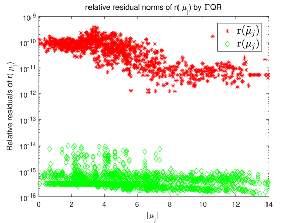
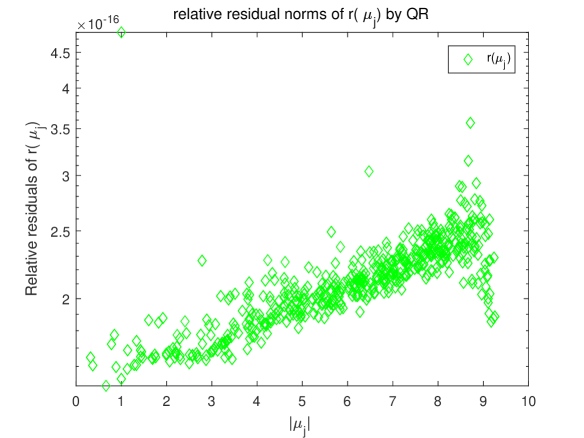
Figure 1: Normalize residual norms for approximate eigenpairs by $\mathrm{\Gamma}$QR (left) and by QR (right)

Example 5.2

In this example, we borrow the first $10000$ rows and columns of 3Dspectralwave2, which is Hermitian, to construct $A$, and the first $10000$ of dielFilterV3clx, which is complex symmetric, to form $B$, leading to $\mathscr{H}\in\mathbb{C}^{20000\times 20000}$. Here, both A and B are sparse matrices. We apply the $\mathrm{\Gamma}$-Lanczos algorithm and the classical Arnoldi method to compute the largest two eigenvalues of $\mathscr{H}^{-1}$ in absolute value, or equivalently, the smallest two eigenvalues of $\mathscr{H}$ in absolute value. In practice, we solve a linear system to calculate $\mathscr{H}^{-1}q$.

Table 3 gives the executing time for both methods, showing that the $\mathrm{\Gamma}$-Lanczos decomposition takes much less time than the Arnoldi decomposition. Table 4 gives the eigenvalues computed by our $\mathrm{\Gamma}$-Lanczos algorithm and the Arnoldi method, where those obtained by the $\mathrm{\Gamma}$-Lanczos algorithm preserve the special structure of the eigenvalues of the initial matrix $\mathscr{H}$, that is, complex eigenvalues appear in quadruples. Besides, the Arnoldi method needs to compute all eight eigenvalues, while our $\mathrm{\Gamma}$-Lanczos algorithm just needs compute two eigenvalues for it.

Table 3: The executing time by the $\mathrm{\Gamma}$-Lanczos algorithm and the Arnoldi method

Method	Phase		Time (secs.)
$\mathrm{\Gamma}$-Lanczos	i	$\mathrm{\Gamma}$-Lanczos decomposition of $\mathscr{H}$	899.9
	ii	Implicit $\mathrm{\Gamma}$QR algorithm	0.9648
Arnoldi	i	Arnoldi decomposition of $\mathscr{H}$	1484.8
	ii	QR method	1.6170

Table 4: The minimum eigenvalues in absolute value

		The smallest two eigenvalues in moduli
$\mathrm{\Gamma}$-Lanczos	$\mu_{1}$	0.0064+0.0117i	0.0064-0.0117i	-0.0064+0.0117i	-0.0064-0.0117i
	$\mu_{2}$	0.0065+0.0202i	0.0065-0.0202i	-0.0065+0.0202i	-0.0065-0.0202i
Arnoldi	$\mu_{1}$	-0.0064-0.0117i	0.0063-0.0118i	-0.0063+0.0107i	0.0064+0.0207i
	$\mu_{2}$	0.0066+0.0117i	-0.0068+0.0203i	0.0065-0.0203i	-0.0068-0.0026i

Figures 2 and 3 display the numerical results of $e(\mu_{j})$ and $r(\mu_{j},\boldsymbol{z}_{j})$, respectively, for $j=1,2$, where the $x$-axis denotes the steps of iteration (writing as $k$), and the $y$-axes, respectively, denote the values of $e(\mu_{j})$ and $r(\mu_{j},\boldsymbol{z}_{j})$. Clearly, $e(\mu_{j})$ and $r(\mu_{j},\boldsymbol{z}_{j})$ from the $\mathrm{\Gamma}$-Lanczos algorithm decrease much faster than those from the Arnoldi method, even $r(\mu_{j},\boldsymbol{z}_{j})$ acquired by our algorithm is square smaller than that by the Arnoldi method. Besides, it is worthwhile to point that when using $r(\mu_{j},\boldsymbol{z}_{j})$ as the stop criterion and setting the tolerance as $r(\mu_{j},\boldsymbol{z}_{j})\leq 10^{-12}$, our $\mathrm{\Gamma}$-Lanczos  algorithm and the Arnoldi method, respectively, require $15$ and $30$ iterations for $\mu_{1}$, and $17$ and $42$ for $\mu_{2}$.

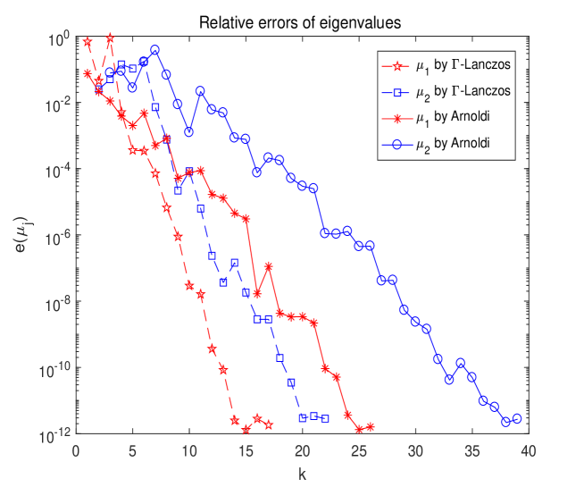
Figure 2: Relative error of eigenvalues for $\mathrm{\Gamma}$-Lanczos and Arnoldi

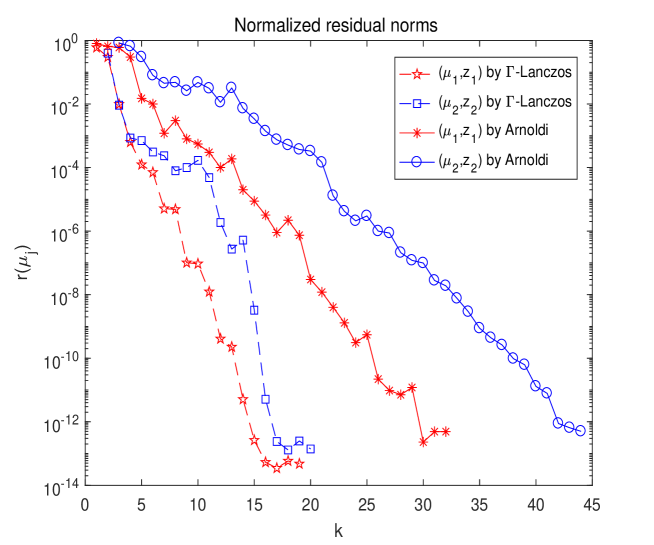
Figure 3: Normalized residual norms for $\mathrm{\Gamma}$-Lanczos and Arnoldi

6 Conclusions

Based on the $\mathrm{\Gamma}$QR  algorithm in [16] for solving the linear response eigenvalue problem, an efficient implicit multishift $\mathrm{\Gamma}$QR  algorithm is extended to solve the Bethe-Salpeter eigenvalue problem with modest size, which preserves the $\Pi^{-}$-Hermitian structure of the initial $\mathscr{H}$. Considering the large-scale Bethe-Salpeter eigenvalue problem, a $\mathrm{\Gamma}$-Lanczos  algorithm is developed, where the adopted special projection gives arise a small size matrix of the $\Pi^{-}$-Hermitian type, which actually is similar to the Rayleigh Quotient in the classical Lanczos method. By computing the eigenvalues of the resulted small size matrix, good approximations of the eigenpairs of $\mathscr{H}$ can be obtained. Essentially, the key of both proposed algorithms is to construct some $\mathrm{\Gamma}$-unitary transformations which preserve the special structure of the eigenpairs of $\mathscr{H}$, guaranteeing the computed eigenpairs appear pairwise as $\{(\lambda,\bm{x}),(-\overline{\lambda},\Pi\overline{\bm{x}})\}$. Numerical experiments show that our $\mathrm{\Gamma}$QR algorithm and $\mathrm{\Gamma}$-Lanczos algorithm respectively take much less executing time than the QR method and the Arnoldi method, to achieve the same relative accuracy of the approximate eigenvalue and also the same relative error of the approximate eigenpair.

References

• [1] M. S. Dresselhaus, G. Dresselhaus, R. Saito, A. Jorio, Exciton photophysics of carbon nanotubes, Annual Review of Physical Chemistry 58 (2007) 719–747.
• [2] R. Barbieri, E. Remiddi, Solving the Bethe-Salpeter equation for positronium, Nuclear Physics B 141 (4) (1978) 413–422.
• [3] G. Onida, L. Reining, A. Rubio, Electronic excitations: density-functional versus many-body green’s-function approaches, Rev. Mod. Phys. 74 (2002) 601–659.
• [4] M. E. Casida, Time-dependent density-functional theory for molecules and molecular solids, J. Molecular Struct.: THEOCHEM 914 (2009) 3–18.
• [5] R. M. Parrish, E. G. Hohenstein, N. Schunck, C. Sherrill, T. J. Martinez, Exact tensor hypercontraction: a universal technique for the resolution of matrix elements of local finite-range N-body potentials in many-body quantum problems, Phys. Rev. Lett. 111 (13) (2013) 132505.
• [6] E. Rebolini, J. Toulouse, A. Savin, Electronic excitation energies of molecular systems from the Bethe-Salpeter equation: Example of the H2 molecule, arXiv e-prints (arXiv:1304.1314).
• [7] Y. Saad, J. R. Chelikowsky, S. M. Shontz, Numerical methods for electronic structure calculations of materials, SIAM Rev. 52 (2010) 3–54.
• [8] D. Rocca, D. Lu, G. Galli, Ab initio calculations of optical absorpation spectra: solution of the Bethe-Salpeter equation within density matrix perturbation theory, J. Chem. Phys. 133 (16) (2010) 164109.
• [9] M. E. Casida, Time-dependent density-functional response theory for molecules, in: D. P. Chong (Ed.), Recent advances in Density Functional Methods, World Scientific, Singapore, 1995, pp. 155–189.
• [10] M. Shao, F. H. D. Jornada, C. Yang, J. Deslippe, S. G. Louie, Structure preserving parallel algorithms for solving the Bethe-Salpeter eigenvalue problem, Linear Algebra Appl. 488 (2016) 148–167.
• [11] P. Benner, V. Khoromskaia, B. N. Khoromskij, A reduced basis approach for calculation of the Bethe-Salpeter excitation energies using low-rank tensor factorizations, Mol. Phys. 114 (7-8) (2016) 1148–1161.
• [12] P. Benner, S. Dolgov, V. Khoromskaia, B. N. Khoromskij, Fast iterative solution of the Bethe-Salpeter eigenvalue problem using low-rank and QTT tensor approximation, J. Comput. Phys. 334 (2017) 221–239.
• [13] Z. Bai, R.-C. Li, Minimization principle for linear response eigenvalue problem, I: Theory, SIAM J. Matrix Anal. Appl. 33 (4) (2012) 1075–1100.
• [14] Z. Bai, R.-C. Li, Minimization principles for the linear response eigenvalue problem II: Computation, SIAM J. Matrix Anal. Appl. 34 (2) (2013) 392–416.
• [15] Z. Teng, R.-C. Li, Convergence analysis of Lanczos-type methods for the linear response eigenvalue problem, J. Comput. Appl. Math. 247 (2013) 17–33.
• [16] T. Li, R.-C. Li, W.-W. Lin, A symmetric structure-preserving $\Gamma$QR algorithm for linear response eigenvalue problems, Linear Algebra Appl. 520 (2017) 191–214.
• [17] J. Demmel, Applied Numerical Linear Algebra, SIAM, Philadelphia, PA, 1997.
• [18] G. H. Golub, C. F. Van Loan, Matrix Computations, 3rd Edition, Johns Hopkins University Press, Baltimore, Maryland, 1996.
• [19] Y. Saad, Numerical methods for large eigenvalue problems, revised version Edition, no. 66 in Classics in Applied Mathematics, SIAM, 2011.
• [20] S. Kaniel, Estimates for some computational techniques in linear algebra, Math. Comp. 20 (95) (1966) 369–378.
• [21] C. C. Paige, The computation of eigenvalues and eigenvectors of very large sparse matirces, Ph.D. thesis, London University, London, England (1971).
• [22] Y. Saad, On the rates of convergence of the Lanczos and the block-Lanczos method, SIAM J. Numer. Anal. 15 (5) (1980) 687–706.
• [23] P. N. Swarztrauber, A direct mehtod for the discrete solution of separable elliptic equations, SIAM J. Nomer. Anal. 11 (1974) 1136–1150.
• [24] G. D. Smith, Numerical Solution of Partial Differential Equations, 2nd Edition, Clarendon Press, Oxford, 1978.
• [25] R. Sweet, Direct methods for the solution of poisson’s equation on a staggered grid, J. Comput. Phys. 12 (1973) 422–428.
• [26] P. N. Swarztrauber, The methods of cyclic reduction, Fourier analysis and cyclic reduction Fourier analysis for the discrete solution of poisson’s equation on a rectangle, SIAM Rev. 19 (1977) 490–501.
• [27] A. Luati, T. Proietti, On the spectral properties of matrices associated with trend filters, Econometric Theory 26 (2010) 1247–1261.
• [28] J. S. Respondek, Numerical simulation in the partial differential equation controllability analysis with physically meaningful constraints, Math. Comput. Simulation 81 (1) (2010) 120–132.
• [29] A. Bunse-Gerstner, An analysis of the HR algorithm for computing the eigenvalues of a matrix, Linear Algebra Appl. 35 (1981) 155–173.
• [30] U. Flaschka, W.-W. Lin, J.-L. Wu, A KQZ algorithm for solving linear-response eigenvalue equations, Linear Algebra Appl. 165 (1992) 93–123.
• [31] S. T. Alexander, C.-T. Pan, R. J. Plemmons, Analysis of a recursive least squares hyperbolic rotation algorithm for signal processing, Linear Algebra Appl. 98 (1988) 3–40.
• [32] G. W. Stewart, J.-G. Sun, Matrix Perturbation Theory, Academic Press, Boston, 1990.