Optimal Bayesian Transfer Learning

Abstract

Transfer learning has recently attracted significant research attention, as it simultaneously learns from different source domains, which have plenty of labeled data, and transfers the relevant knowledge to the target domain with limited labeled data to improve the prediction performance. We propose a Bayesian transfer learning framework, in the homogeneous transfer learning scenario, where the source and target domains are related through the joint prior density of the model parameters. The modeling of joint prior densities enables better understanding of the “transferability” between domains. We define a joint Wishart distribution for the precision matrices of the Gaussian feature-label distributions in the source and target domains to act like a bridge that transfers the useful information of the source domain to help classification in the target domain by improving the target posteriors. Using several theorems in multivariate statistics, the posteriors and posterior predictive densities are derived in closed forms with hypergeometric functions of matrix argument, leading to our novel closed-form and fast Optimal Bayesian Transfer Learning (OBTL) classifier. Experimental results on both synthetic and real-world benchmark data confirm the superb performance of the OBTL compared to the other state-of-the-art transfer learning and domain adaptation methods.

I Introduction

A basic assumption of traditional machine learning is that data in the training and test sets are independently sampled in one domain with the identical underlying distribution. However, with the growing amount of heterogeneity in modern data, the assumption of having only one domain may not be reasonable. Transfer learning (TL) is a learning strategy that enables us to learn from a source domain with plenty of labeled data as well as a target domain with no or very few labeled data in order to design a better classifier in the target domain than the ones trained by target-only data for its generalization performance. This can reduce the effort of collecting labeled data for the target domain, which might be very costly, if not impossible. Due to its importance, there has been ongoing research on the topic of transfer learning and many surveys in the recent years covering transfer learning and domain adaptation methods from different perspectives [1, 2, 3, 4, 5].

If we train a model in one domain and directly apply it in another, the trained model may not generalize well, but if the domains are related, appropriate transfer learning and domain adaptation methods can borrow information from all the data across the domains to develop better generalizable models in the target domain. Transfer learning in medical genomics is desirable, since the number of labeled data samples is often very limited due to the difficulty of having disease samples and the prohibitive costs of human clinical trials. However, it is relatively easier to obtain gene-expression data for cell lines or other model species like mice or dogs. If these different life systems share the same underlying disease cellular mechanisms, we may utilize data in cell lines or model species as our source domain to develop transfer learning methods for more accurate human disease prognosis in the target domain [6, 7].

I-A Related Works

Domain adaptation (DA) is a specific case of transfer learning where the source and target domains have the same classes or categories [2, 3, 5]. DA methods either adapt the model learned in the source domain to be applied in the target domain or adapt the source data so that the distribution can be close to the one of the target data. Depending on the availability of labeled target data, the DA methods are categorized as unsupervised and semi-supervised algorithms. Unsupervised DA problems applies to the cases where there are no labeled target data and the algorithm uses only unlabeled data in the target domain along with source labeled data [8]. Semi-supervised DA methods use both the unlabeled and a few labeled target data to learn a classifier in the target domain with the help of source labeled data [9, 10, 11, 12].

Depending on whether the source and target domains have the same feature space with the same feature dimension, there are homogeneous and heterogeneous DA methods. The first direction in homogeneous DA is instance re-weighting, for which the most popular measure to re-weight the data is Maximum Mean Discrepancy (MMD) [13] between the two domains. Transfer Adaptive Boosting (TrAdaBoost) [14] is another method that adaptively sets the weights for the source and target samples during each iteration based on the relevance of source and target data to help train the target classifier. Another direction is model or parameter adaptation. There are several efforts to adapt the SVM classifier designed in the source domain for the target domain, for example, based on residual error [15, 16]. Feature augmentation methods, such as Geodesic Flow Sampling (GFS) and Geodesic Flow Kernel (GFK) [8], derive intermediate subspaces using Geodesic flows, which interpolate between the source and target domains. Finding an invariant latent domain in which the distance between the empirical distributions of the source and target data is minimized is another direction to tackle the problem of domain adaptation, such as Invariant Latent Space (ILS) in [17]. Authors in [17] proposed to learn an invariant latent Hilbert space to address both the unsupervised and semi-supervised DA problems, where a notion of domain variance is simultaneously minimized while maximizing a measure of discriminatory power using Riemannian optimization techniques. Max-Margin Domain Transform (MMDT) [10] is a semi-supervised feature transformation DA method which uses a cost function based on the misclassification loss and jointly optimizes both the transformation and classifier parameters. Another domain-invariant representation method [18] matches the distributions in the source and target domains via a regularized optimal transportation model. Heterogeneous Feature Augmentation (HFA) [9] is a heterogeneous DA method which typically embeds the source and target data into a common latent space prior to data augmentation.

Domain adaption has been recently studied in deep learning frameworks like deep adaptation network (DAN) [19], residual transfer networks (RTN) [20], and models based on generative adversarial networks (GAN) such as domain adversarial neural network (DaNN) [21] and coupled GAN (CoGAN) [22]. Although deep DA methods have shown promising results, they require a fairly large amount of labeled data.

I-B Main Contributions

This paper treats homogeneous transfer learning and domain adaptation from Bayesian perspectives, a key aim being better theoretical understanding when data in the source domain are “transferrable” to help learning in the target domain. When learning complex systems with limited data, Bayesian learning can integrate prior knowledge to compensate for the generalization performance loss due to the lack of data. Rooted in Optimal Bayesian Classifiers (OBC) [23, 24], which gives the classifiers having Bayesian minimum mean squared error (MMSE) over uncertainty classes of feature-label distributions, we propose a Bayesian transfer learning framework and the corresponding Optimal Bayesian Transfer Learning (OBTL) classifier to formulate the OBC in the target domain by taking advantage of both the available data and the joint prior knowledge in source and target domains. In this Bayesian learning framework, transfer learning from the source to target domain is through a joint prior probability density function for the model parameters of the feature-label distributions of the two domains. By explicitly modeling the dependency of the model parameters of the feature-label distribution, the posterior of the target model parameters can be updated via the joint prior probability distribution function in conjunction with the source and target data. Based on that, we derive the effective class-conditional densities of the target domain, by which the OBTL classifier is constructed.

Our problem definition is the same as the aforementioned domain adaptation methods, where there are plenty of labeled source data and few labeled target data. The source and target data follow different multivariate Gaussian distributions with arbitrary mean vectors and precision (inverse of covariance) matrices. For the OBTL, we define a joint Gaussian-Wishart prior distribution, where the two precision matrices in the two domains are jointly connected. This joint prior distribution for the two precision matrices of the two domains acts like a bridge through which the useful knowledge of the source domain can be transferred to the target domain, making the posterior of the target parameters tighter with less uncertainty.

With such a Bayesian transfer learning framework and several theorems from multivariate statistics, we define an appropriate joint prior for the precision matrices using hypergeometric functions of matrix argument, whose marginal distributions are Wishart as well. The corresponding closed-form posterior distributions for the target model parameters are derived by integrating out all the source model parameters. Having closed-form posteriors facilitates closed-form effective class-conditional densities. Hence, the OBTL classifier can be derived based on the corresponding hypergeometric functions and does not need iterative and costly techniques like MCMC sampling. Although the OBTL classifier has a closed form, computing these hypergeometric functions involves the computation of series of zonal polynomials, which is time-consuming and not scalable to high dimension. To resolve this issue, we use the Laplace approximations of these functions, which preserves the good prediction performance of the OBTL while making it efficient and scalable. The performance of the OBTL is tested on both synthetic data and real-world benchmark image datasets to show its superior performance over state-of-the-art domain adaption methods.

The paper is organized as follows. Section II introduces the Bayesian transfer learning framework. Section III derives the closed-form posteriors of target parameters, via which Section IV obtains the effective class-conditional densities in the target domain. Section V derives the OBTL classifier, and Section VI presents the OBC in the target domain and shows that the OBTL classifier converts to the target-only OBC when there is no interaction between the domains. Section VII presents experimental results using both synthetic and real-world benchmark data. Section VIII concludes the paper. Appendix A states some useful theorems for the generalized hypergeometric functions of matrix argument. Appendices B and C provide the proofs of our main theorems. Finally, Appendix D presents the Laplace approximation of Gauss hypergeometric functions of matrix argument.

II Bayesian Transfer Learning Framework

We consider a supervised transfer learning problem in which there are $L$ common classes (labels) in each domain. Let $\mathcal{D}_{s}$ and $\mathcal{D}_{t}$ denote the labeled datasets of the source and target domains with the sizes of $N_{s}$ and $N_{t}$, respectively, where $N_{t}\ll N_{s}$. Let $\mathcal{D}_{s}^{l}=\left\{\mathbf{x}_{s,1}^{l},\mathbf{x}_{s,2}^{l},\cdots,\mathbf{x}_{s,n_{s}^{l}}^{l}\right\}$, $l\in\{1,\cdots,L\}$, where $n_{s}^{l}$ denotes the size of data in the source domain for the label $l$. Similarly, let $\mathcal{D}_{t}^{l}=\left\{\mathbf{x}_{t,1}^{l},\mathbf{x}_{t,2}^{l},\cdots,\mathbf{x}_{t,n_{t}^{l}}^{l}\right\}$, $l\in\{1,\cdots,L\}$, where $n_{t}^{l}$ denotes the size of data in the target domain for the label $l$. There is no intersection between $\mathcal{D}_{t}^{i}$ and $\mathcal{D}_{t}^{j}$ and also between $\mathcal{D}_{s}^{i}$ and $\mathcal{D}_{s}^{j}$ for any $i,j\in\{1,\cdots,L\}$. Obviously, we have $\mathcal{D}_{s}=\cup_{l=1}^{L}\mathcal{D}_{s}^{l}$, $\mathcal{D}_{t}=\cup_{l=1}^{L}\mathcal{D}_{t}^{l}$, $N_{s}=\sum_{l=1}^{L}n_{s}^{l}$, and $N_{t}=\sum_{l=1}^{L}n_{t}^{l}$. Since we consider the homogeneous transfer learning scenario, where the feature spaces are the same in both the source and target domains, $\mathbf{x}_{s}^{l}$ and $\mathbf{x}_{t}^{l}$ are $d\times 1$ vectors for $d$ features of the source and target domains, respectively.

Letting $\mathbf{x}^{l}=\left[{\mathbf{x}_{t}^{l^{\prime}}},{\mathbf{x}_{s}^{l^{\prime}}}\right]^{\prime}$ be a $2d\times 1$ augmented feature vector, $\mathbf{A}^{{}^{\prime}}$ denoting the transpose of matrix $\mathbf{A}$, a general joint sampling model would take the Gaussian form

$$\mathbf{x}^{l}\sim\mathcal{N}\left(\mathbf{\mu}^{l},\left(\mathbf{\Lambda}^{l}\right)^{-1}\right),\leavevmode\nobreak\ \leavevmode\nobreak\ \leavevmode\nobreak\ l\in\{1,\cdots,L\},$$ (1)

with

$$\mathbf{\mu}^{l}=\begin{bmatrix}\mathbf{\mu}_{t}^{l}\\ \mathbf{\mu}_{s}^{l}\end{bmatrix},\leavevmode\nobreak\ \leavevmode\nobreak\ \leavevmode\nobreak\ \leavevmode\nobreak\ \mathbf{\Lambda}^{l}=\begin{bmatrix}\mathbf{\Lambda}_{t}^{l}&\mathbf{\Lambda}_{ts}^{l}\\ {\mathbf{\Lambda}_{ts}^{l}}^{{}^{\prime}}&\mathbf{\Lambda}_{s}^{l}\end{bmatrix},$$ (2)

where $\mathbf{\mu}^{l}$ is the $2d\times 1$ mean vector, and $\mathbf{\Lambda}^{l}$ is the $2d\times 2d$ precision matrix. In this model, $\mathbf{\Lambda}_{t}^{l}$ and $\mathbf{\Lambda}_{s}^{l}$ account for the interactions of features within the source and target domains, respectively, and $\mathbf{\Lambda}_{ts}^{l}$ accounts for the interactions of the features across the source and target domains, for any class $l\in\{1,\cdots,L\}$. In this Gaussian setting, it is common to use a Wishart distribution as a prior for the precision matrix $\mathbf{\Lambda}^{l}$, since it is a conjugate prior.

In transfer learning, it is not realistic to assume joint sampling of the source and target domains. Therefore we cannot use the general joint sampling model. Instead, we assume that there are two datasets separately sampled from the source and target domains. Thus, we define a joint prior distribution for $\mathbf{\Lambda}_{s}^{l}$ and $\mathbf{\Lambda}_{t}^{l}$ by marginalizing out the term $\mathbf{\Lambda}_{ts}^{l}$. This joint prior distribution of the parameters of the source and target domains accounts for the dependency (or “relatedness”) between the domains.

Given this adjustment to account for transfer learning, we utilize a Gaussian model for the feature-label distribution in each domain:

$$\mathbf{x}_{z}^{l}\sim\mathcal{N}\left(\mathbf{\mu}_{z}^{l},{\left(\mathbf{\Lambda}_{z}^{l}\right)}^{-1}\right),\leavevmode\nobreak\ \leavevmode\nobreak\ \leavevmode\nobreak\ l\in\{1,\cdots,L\},$$ (3)

where subscript $z\in\{s,t\}$ denotes the source $s$ or target $t$ domain, $\mathbf{\mu}_{s}^{l}$ and $\mathbf{\mu}_{t}^{l}$ are $d\times 1$ mean vectors in the source and target domains for label $l$, respectively, $\mathbf{\Lambda}_{s}^{l}$ and $\mathbf{\Lambda}_{t}^{l}$ are the $d\times d$ precision matrices in the source and target domains for label $l$, respectively, and a joint Gaussian-Wishart distribution is employed as a prior for mean and precision matrices of the Gaussian models. Under these assumptions, the joint prior distribution for $\mathbf{\mu}_{s}^{l}$, $\mathbf{\mu}_{t}^{l}$, $\mathbf{\Lambda}_{s}^{l}$, and $\mathbf{\Lambda}_{s}^{l}$ takes the form

$$p\left(\mathbf{\mu}_{s}^{l},\mathbf{\mu}_{t}^{l},\mathbf{\Lambda}_{s}^{l},\mathbf{\Lambda}_{t}^{l}\right)=p\left(\mathbf{\mu}_{s}^{l},\mathbf{\mu}_{t}^{l}|\mathbf{\Lambda}_{s}^{l},\mathbf{\Lambda}_{t}^{l}\right)p\left(\mathbf{\Lambda}_{s}^{l},\mathbf{\Lambda}_{t}^{l}\right).$$ (4)

To facilitate conjugate priors, we assume that, for any class $l\in\{1,\cdots,L\}$, $\mathbf{\mu}_{s}^{l}$ and $\mathbf{\mu}_{t}^{l}$ are conditionally independent given $\mathbf{\Lambda}_{s}^{l}$ and $\mathbf{\Lambda}_{t}^{l}$, so that

$$p\left(\mathbf{\mu}_{s}^{l},\mathbf{\mu}_{t}^{l},\mathbf{\Lambda}_{s}^{l},\mathbf{\Lambda}_{t}^{l}\right)=p\left(\mathbf{\mu}_{s}^{l}|\mathbf{\Lambda}_{s}^{l}\right)p\left(\mathbf{\mu}_{t}^{l}|\mathbf{\Lambda}_{t}^{l}\right)p\left(\mathbf{\Lambda}_{s}^{l},\mathbf{\Lambda}_{t}^{l}\right),$$ (5)

and that both $p\left(\mathbf{\mu}_{s}^{l}|\mathbf{\Lambda}_{s}^{l}\right)$ and $p\left(\mathbf{\mu}_{t}^{l}|\mathbf{\Lambda}_{t}^{l}\right)$ are Gaussian,

$$\mathbf{\mu}_{z}^{l}|\mathbf{\Lambda}_{z}^{l}\sim\mathcal{N}\left(\mathbf{m}_{z}^{l},\left(\kappa_{z}^{l}\mathbf{\Lambda}_{z}^{l}\right)^{-1}\right),$$ (6)

where $\mathbf{m}_{z}^{l}$ is the $d\times 1$ mean vector of $\mathbf{\mu}_{z}^{l}$, and $\kappa_{z}^{l}$ is a positive scalar hyperparameter. We need to define a joint distribution for $\mathbf{\Lambda}_{s}^{l}$ and $\mathbf{\Lambda}_{t}^{l}$. In the case of a prior for either $\mathbf{\Lambda}_{s}^{l}$ or $\mathbf{\Lambda}_{t}^{l}$, we use a Wishart distribution as the conjugate prior. Here we desire a joint distribution for $\mathbf{\Lambda}_{s}^{l}$ and $\mathbf{\Lambda}_{t}^{l}$, whose marginal distributions for both $\mathbf{\Lambda}_{s}^{l}$ and $\mathbf{\Lambda}_{t}^{l}$ are Wishart.

We present some definitions and theorems that will be used in deriving the OBTL classifier.

Definition 1.

A random $d\times d$ symmetric positive-definite matrix $\mathbf{\Lambda}$ has a nonsingular Wishart distribution with $\nu$ degrees of freedom, $W_{d}(\mathbf{M},\nu)$, if $\nu\geq d$ and $\mathbf{M}$ is a $d\times d$ positive-definite matrix ($\mathbf{M}>0$) and the density is

$$p(\mathbf{\Lambda})=\left[2^{\frac{\nu d}{2}}\Gamma_{d}\left(\frac{\nu}{2}\right)|\mathbf{M}|^{\frac{\nu}{2}}\right]^{-1}|\mathbf{\Lambda}|^{\frac{\nu-d-1}{2}}\mathrm{etr}\left(-\frac{1}{2}\mathbf{M}^{-1}\mathbf{\Lambda}\right),$$ (7)

where $|\mathbf{A}|$ is the determinant of $\mathbf{A}$, $\mathrm{etr}(\mathbf{A})=\exp\left(\mathrm{tr}(\mathbf{A})\right)$ and $\Gamma_{d}(\alpha)$ is the multivariate gamma function given by

$$\Gamma_{d}(\alpha)=\pi^{\frac{d(d-1)}{4}}\prod_{i=1}^{d}\Gamma\left(\alpha-\frac{i-1}{2}\right).$$ (8)

Proposition 1.

[25]: If $\mathbf{\Lambda}\sim W_{d}(\mathbf{M},\nu)$, and $\mathbf{A}$ is an $r\times d$ matrix of rank $r$, where $r\leq d$, then $\mathbf{A}\mathbf{\Lambda}\mathbf{A}^{{}^{\prime}}\sim W_{r}(\mathbf{A}\mathbf{M}\mathbf{A}^{{}^{\prime}},\nu)$.

Corollary 1.

If $\mathbf{\Lambda}\sim W_{d}(\mathbf{M},\nu)$ and $\mathbf{\Lambda}=\begin{pmatrix}\mathbf{\Lambda}_{11}&\mathbf{\Lambda}_{12}\\ \mathbf{\Lambda}_{12}^{{}^{\prime}}&\mathbf{\Lambda}_{22}\end{pmatrix}$, where $\mathbf{\Lambda}_{11}$ and $\mathbf{\Lambda}_{22}$ are $d_{1}\times d_{1}$ and $d_{2}\times d_{2}$ submatrices, respectively, and if $\mathbf{M}=\begin{pmatrix}\mathbf{M}_{11}&\mathbf{M}_{12}\\ \mathbf{M}_{12}^{{}^{\prime}}&\mathbf{M}_{22}\end{pmatrix}$ is the corresponding partition of $\mathbf{M}$ with $\mathbf{M}_{11}$ and $\mathbf{M}_{22}$ being two $d_{1}\times d_{1}$ and $d_{2}\times d_{2}$ submatrices, respectively, then $\mathbf{\Lambda}_{11}\sim W_{d_{1}}(\mathbf{M}_{11},\nu)$ and $\mathbf{\Lambda}_{22}\sim W_{d_{2}}(\mathbf{M}_{22},\nu)$.

Using Corollary 1, we can ensure that using the Wishart distribution for the precision matrix $\mathbf{\Lambda}^{l}$ (2) of the joint model in (1) will lead to the Wishart marginal distributions for $\mathbf{\Lambda}_{s}^{l}$ and $\mathbf{\Lambda}_{t}^{l}$ in the source and target domains separately, which is a desired property. Now we introduce a theorem, proposed in [26], which gives the form of the joint distribution of the two submatrices of a partitioned Wishart matrix.

Theorem 1.

[26]: Let $\mathbf{\Lambda}=\begin{pmatrix}\mathbf{\Lambda}_{11}&\mathbf{\Lambda}_{12}\\ \mathbf{\Lambda}_{12}^{{}^{\prime}}&\mathbf{\Lambda}_{22}\end{pmatrix}$ be a $(d_{1}+d_{2})\times(d_{1}+d_{2})$ partitioned Wishart random matrix, where the diagonal partitions are of sizes $d_{1}\times d_{1}$ and $d_{2}\times d_{2}$, respectively. The Wishart distribution of $\mathbf{\Lambda}$ has $\nu\geq d_{1}+d_{2}$ degrees of freedom and positive-definite scale matrix $\mathbf{M}=\begin{pmatrix}\mathbf{M}_{11}&\mathbf{M}_{12}\\ \mathbf{M}_{12}^{{}^{\prime}}&\mathbf{M}_{22}\end{pmatrix}$ partitioned in the same way as $\mathbf{\Lambda}$. The joint distribution of the two diagonal partitions $\mathbf{\Lambda}_{11}$ and $\mathbf{\Lambda}_{22}$ have the density function given by

$$p(\mathbf{\Lambda}_{11},\mathbf{\Lambda}_{22})=$$ (9)

$$K\leavevmode\nobreak\ \mathrm{etr}\left(-\frac{1}{2}\left(\mathbf{M}_{11}^{-1}+\mathbf{F}^{{}^{\prime}}\mathbf{C}_{2}\mathbf{F}\right)\mathbf{\Lambda}_{11}\right)\mathrm{etr}\left(-\frac{1}{2}\mathbf{C}_{2}^{-1}\mathbf{\Lambda}_{22}\right)$$

$$\times|\mathbf{\Lambda}_{11}|^{\frac{\nu-d_{2}-1}{2}}\leavevmode\nobreak\ |\mathbf{\Lambda}_{22}|^{\frac{\nu-d_{1}-1}{2}}\leavevmode\nobreak\ \leavevmode\nobreak\ _{0}F_{1}\left(\frac{\nu}{2};\frac{1}{4}\mathbf{G}\right),$$

where $\mathbf{C}_{2}=\mathbf{M}_{22}-\mathbf{M}_{12}^{{}^{\prime}}\mathbf{M}_{11}^{-1}\mathbf{M}_{12}$, $\mathbf{F}=\mathbf{C}_{2}^{-1}\mathbf{M}_{12}^{{}^{\prime}}\mathbf{M}_{11}^{-1}$, $\mathbf{G}=\mathbf{\Lambda}_{22}^{\frac{1}{2}}\mathbf{F}\mathbf{\Lambda}_{11}\mathbf{F}^{{}^{\prime}}\mathbf{\Lambda}_{22}^{\frac{1}{2}}$, $K^{-1}=2^{\frac{(d_{1}+d_{2})\nu}{2}}\Gamma_{d_{1}}\left(\frac{\nu}{2}\right)\Gamma_{d_{2}}\left(\frac{\nu}{2}\right)|\mathbf{M}|^{\frac{\nu}{2}}$, and$\leavevmode\nobreak\ {}_{0}F_{1}$ is the generalized matrix-variate hypergeometric function.

Definition 2.

[27]: The generalized hypergeometric function of one matrix argument is defined by

$$\leavevmode\nobreak\ {}_{p}F_{q}(a_{1},\cdots,a_{p};b_{1},\cdots,b_{q};\mathbf{X})\hskip 56.9055pt$$

$$=\sum_{k=0}^{\infty}\sum_{\kappa\vdash k}\frac{(a_{1})_{\kappa}\cdots(a_{p})_{\kappa}}{(b_{1})_{\kappa}\cdots(b_{q})_{\kappa}}\frac{C_{\kappa}(\mathbf{X})}{k!},$$ (10)

where $a_{i}$, $i=1,\cdots,p$, and $b_{j}$, $j=1,\cdots,q$, are arbitrary complex (real in our case) numbers, $C_{\kappa}(\mathbf{X})$ is the zonal polynomial of $d\times d$ symmetric matrix $\mathbf{X}$ corresponding to the ordered partition $\kappa=(k_{1},\cdots,k_{d})$, $k_{1}\geq\cdots\geq k_{d}\geq 0$, $k_{1}+\cdots k_{d}=k$ and $\sum_{\kappa\vdash k}$ denotes summation over all partitions $\kappa$ of $k$. The generalized hypergeometric coefficient $(a)_{\kappa}$ is defined by

$$(a)_{\kappa}=\prod_{i=1}^{d}\left(a-\frac{i-1}{2}\right)_{k_{i}},$$ (11)

where $(a)_{r}=a(a+1)\cdots(a+r-1)$, $r=1,2,\cdots$, with $(a)_{0}=1$.

Conditions for convergence of the series in (2) are available in the literature [28]. From (2) it follows

$$\leavevmode\nobreak\ {}_{0}F_{0}(\mathbf{X})=\sum_{k=0}^{\infty}\sum_{\kappa\vdash k}\frac{C_{\kappa}(\mathbf{X})}{k!}=\sum_{k=0}^{\infty}\frac{(\mathrm{tr}(\mathbf{X}))^{k}}{k!}=\mathrm{etr}(\mathbf{X}),$$ (12)

$$\leavevmode\nobreak\ {}_{1}F_{0}(a;\mathbf{X})=\sum_{k=0}^{\infty}\sum_{\kappa\vdash k}\frac{(a)_{\kappa}C_{\kappa}(\mathbf{X})}{k!}=|\mathbf{I}_{m}-\mathbf{X}|^{-a},\leavevmode\nobreak\ \leavevmode\nobreak\ ||\mathbf{X}||<1,$$

$$\leavevmode\nobreak\ {}_{0}F_{1}(b;\mathbf{X})=\sum_{k=0}^{\infty}\sum_{\kappa\vdash k}\frac{C_{\kappa}(\mathbf{X})}{(b)_{\kappa}k!},$$

$$\leavevmode\nobreak\ {}_{1}F_{1}(a;b;\mathbf{X})=\sum_{k=0}^{\infty}\sum_{\kappa\vdash k}\frac{(a)_{\kappa}}{(b)_{\kappa}}\frac{C_{\kappa}(\mathbf{X})}{k!},$$

$$\leavevmode\nobreak\ {}_{2}F_{1}(a,b;c;\mathbf{X})=\sum_{k=0}^{\infty}\sum_{\kappa\vdash k}\frac{(a)_{\kappa}(b)_{\kappa}}{(c)_{\kappa}}\frac{C_{\kappa}(\mathbf{X})}{k!},\leavevmode\nobreak\ \leavevmode\nobreak\ \leavevmode\nobreak\ ||\mathbf{X}||<1,$$

where $||\mathbf{X}||<1$ means that the maximum of the absolute values of the eigenvalues of $\mathbf{X}$ is less than $1$. ${}_{1}F_{1}(a;b;\mathbf{X})$ and ${}_{2}F_{1}(a,b;c;\mathbf{X})$ are respectively called Confluent and Gauss hypergeometric functions of matrix argument. See Appendix A for some useful theorems on zonal polynomials and generalized hypergeometric functions of matrix arguments. We use those theorems to derive the posterior densities and posterior predictive densities of the target parameters in closed forms in terms of Confluent and Gauss hypergeometric functions of matrix argument in Sections III and IV, respectively.

Now, using Theorem 1, we define the joint prior distribution, $p(\mathbf{\Lambda}_{s}^{l},\mathbf{\Lambda}_{t}^{l})$ in (5), of the precision matrices of the source and target domains for class $l\in\{1,\cdots,L\}$ as follows:

$$p(\mathbf{\Lambda}_{t}^{l},\mathbf{\Lambda}_{s}^{l})=K^{l}\mathrm{etr}\left(-\frac{1}{2}\left({\left(\mathbf{M}_{t}^{l}\right)}^{-1}+{\mathbf{F}^{l}}^{{}^{\prime}}\mathbf{C}^{l}\mathbf{F}^{l}\right)\mathbf{\Lambda}_{t}^{l}\right)$$ (13)

$$\times\mathrm{etr}\left(-\frac{1}{2}{\left(\mathbf{C}^{l}\right)}^{-1}\mathbf{\Lambda}_{s}^{l}\right)$$

$$\times\left|\mathbf{\Lambda}_{t}^{l}\right|^{\frac{\nu^{l}-d-1}{2}}\left|\mathbf{\Lambda}_{s}^{l}\right|^{\frac{\nu^{l}-d-1}{2}}\leavevmode\nobreak\ _{0}F_{1}\left(\frac{\nu^{l}}{2};\frac{1}{4}\mathbf{G}^{l}\right),$$

where $\mathbf{M}=\begin{pmatrix}\mathbf{M}_{t}^{l}&\mathbf{M}_{ts}^{l}\\ {\mathbf{M}_{ts}^{l}}^{{}^{\prime}}&\mathbf{M}_{s}^{l}\end{pmatrix}$ is a $2d\times 2d$ positive definite scale matrix, $\nu^{l}\geq 2d$ denotes degrees of freedom, and

$$\mathbf{C}^{l} = \mathbf{M}_{s}^{l}-{\mathbf{M}_{ts}^{l}}^{{}^{\prime}}{\left(\mathbf{M}_{t}^{l}\right)}^{-1}\mathbf{M}_{ts}^{l},$$ (14)

$$\mathbf{F}^{l} = {\left(\mathbf{C}^{l}\right)}^{-1}{\mathbf{M}_{ts}^{l}}^{{}^{\prime}}{\left(\mathbf{M}_{t}^{l}\right)}^{-1},$$

$$\mathbf{G}^{l} = {\mathbf{\Lambda}_{s}^{l}}^{\frac{1}{2}}\mathbf{F}^{l}\mathbf{\Lambda}_{t}^{l}{\mathbf{F}^{l}}^{{}^{\prime}}{\mathbf{\Lambda}_{s}^{l}}^{\frac{1}{2}},$$

$${(K^{l})}^{-1} = 2^{d\nu^{l}}\Gamma_{d}^{2}\left(\frac{\nu^{l}}{2}\right)|\mathbf{M}^{l}|^{\frac{\nu^{l}}{2}}.$$

Using Corollary 1, $\mathbf{\Lambda}_{t}^{l}$ and $\mathbf{\Lambda}_{s}^{l}$ have the following Wishart marginal distributions:

$$\mathbf{\Lambda}_{z}^{l}\sim W_{d}(\mathbf{M}_{z}^{l},\nu^{l}),\leavevmode\nobreak\ \leavevmode\nobreak\ \leavevmode\nobreak\ l\in\{1,\cdots,L\},\leavevmode\nobreak\ \leavevmode\nobreak\ \leavevmode\nobreak\ z\in\{s,t\}.$$ (15)

III Posteriors of Target Parameters

Figure 1: Dependency of the source and target domains through their precision matrices for any class $l\in\{1,\cdots,L\}$.

Having defined the prior distributions in the previous section, we aim to derive the posterior distribution of the parameters of the target domain upon observing the training source $\mathcal{D}_{s}$ and target $\mathcal{D}_{t}$ datasets. The likelihood of the datasets $\mathcal{D}_{t}$ and $\mathcal{D}_{s}$ is conditionally independent given the parameters of the target and source domains. The dependence between the two domains is due to the dependence of the prior distributions of the precision matrices, as shown in Fig 1. Within each domain, source or target, the likelihoods of the different classes are also conditionally independent given the parameters of the classes. As such, the joint likelihood of the datasets $\mathcal{D}_{t}$ and $\mathcal{D}_{s}$ can be written as

$$p(\mathcal{D}_{t}, \mathcal{D}_{s}|\mathbf{\mu}_{t},\mathbf{\mu}_{s},\mathbf{\Lambda}_{t},\mathbf{\Lambda}_{s})=p(\mathcal{D}_{t}|\mathbf{\mu}_{t},\mathbf{\Lambda}_{t})p(\mathcal{D}_{s}|\mathbf{\mu}_{s},\mathbf{\Lambda}_{s})$$ (16)

$$=p(\mathcal{D}_{t}^{1},\cdots,\mathcal{D}_{t}^{L}|\mathbf{\mu}_{t}^{1},\cdots,\mathbf{\mu}_{t}^{L},\mathbf{\Lambda}_{t}^{1},\cdots,\mathbf{\Lambda}_{t}^{L})$$

$$\leavevmode\nobreak\ \leavevmode\nobreak\ \leavevmode\nobreak\ \leavevmode\nobreak\ \times p(\mathcal{D}_{s}^{1},\cdots,\mathcal{D}_{s}^{L}|\mathbf{\mu}_{s}^{1},\cdots,\mathbf{\mu}_{s}^{L},\mathbf{\Lambda}_{s}^{1},\cdots,\mathbf{\Lambda}_{s}^{L})$$

$$=\prod_{l=1}^{L}p(\mathcal{D}_{t}^{l}|\mathbf{\mu}_{t}^{l},\mathbf{\Lambda}_{t}^{l})\prod_{l=1}^{L}p(\mathcal{D}_{s}^{l}|\mathbf{\mu}_{s}^{l},\mathbf{\Lambda}_{s}^{l}).$$

The posterior of the parameters given $\mathcal{D}_{t}$ and $\mathcal{D}_{s}$ satisfies

$$p(\mathbf{\mu}_{t},\mathbf{\mu}_{s},\mathbf{\Lambda}_{t},\mathbf{\Lambda}_{s}|\mathcal{D}_{t},\mathcal{D}_{s})$$ (17)

$$\propto p(\mathcal{D}_{t},\mathcal{D}_{s}|\mathbf{\mu}_{t},\mathbf{\mu}_{s},\mathbf{\Lambda}_{t},\mathbf{\Lambda}_{s})p(\mathbf{\mu}_{t},\mathbf{\mu}_{s},\mathbf{\Lambda}_{t},\mathbf{\Lambda}_{s})$$

$$\propto\prod_{l=1}^{L}p(\mathcal{D}_{t}^{l}|\mathbf{\mu}_{t}^{l},\mathbf{\Lambda}_{t}^{l})\prod_{l=1}^{L}p(\mathcal{D}_{s}^{l}|\mathbf{\mu}_{s}^{l},\mathbf{\Lambda}_{s}^{l})\prod_{l=1}^{L}p(\mathbf{\mu}_{t}^{l},\mathbf{\mu}_{s}^{l},\mathbf{\Lambda}_{t}^{l},\mathbf{\Lambda}_{s}^{l}),$$

where we assume that the priors of the parameters in different classes are independent, $p(\mathbf{\mu}_{t},\mathbf{\mu}_{s},\mathbf{\Lambda}_{t},\mathbf{\Lambda}_{s})=\prod_{l=1}^{L}p(\mathbf{\mu}_{t}^{l},\mathbf{\mu}_{s}^{l},\mathbf{\Lambda}_{t}^{l},\mathbf{\Lambda}_{s}^{l})$. From (5) and (17),

$$p(\mu_{t},\mu_{s},\mathbf{\Lambda}_{t},\mathbf{\Lambda}_{s}|\mathcal{D}_{t},\mathcal{D}_{s})\propto\prod_{l=1}^{L}p(\mathcal{D}_{t}^{l}|\mathbf{\mu}_{t}^{l},\mathbf{\Lambda}_{t}^{l})p(\mathcal{D}_{s}^{l}|\mathbf{\mu}_{s}^{l},\mathbf{\Lambda}_{s}^{l})$$ (18)

$$\hskip 28.45274pt\times p\left(\mathbf{\mu}_{s}^{l}|\mathbf{\Lambda}_{s}^{l}\right)p\left(\mathbf{\mu}_{t}^{l}|\mathbf{\Lambda}_{t}^{l}\right)p\left(\mathbf{\Lambda}_{s}^{l},\mathbf{\Lambda}_{t}^{l}\right).$$

We can see that the posterior of the parameters is equal to the product of the posteriors of the parameters of each class:

$$p(\mu_{t},\mu_{s},\mathbf{\Lambda}_{t},\mathbf{\Lambda}_{s}|\mathcal{D}_{t},\mathcal{D}_{s})=\prod_{l=1}^{L}p(\mathbf{\mu}_{t}^{l},\mathbf{\mu}_{s}^{l},\mathbf{\Lambda}_{t}^{l},\mathbf{\Lambda}_{s}^{l}|\mathcal{D}_{t}^{l},\mathcal{D}_{s}^{l}),$$ (19)

where

$$p(\mathbf{\mu}_{t}^{l},\mathbf{\mu}_{s}^{l},\mathbf{\Lambda}_{t}^{l},\mathbf{\Lambda}_{s}^{l}|\mathcal{D}_{t}^{l},\mathcal{D}_{s}^{l})\propto p(\mathcal{D}_{t}^{l}|\mathbf{\mu}_{t}^{l},\mathbf{\Lambda}_{t}^{l})p(\mathcal{D}_{s}^{l}|\mathbf{\mu}_{s}^{l},\mathbf{\Lambda}_{s}^{l})$$

$$\times p\left(\mathbf{\mu}_{s}^{l}|\mathbf{\Lambda}_{s}^{l}\right)p\left(\mathbf{\mu}_{t}^{l}|\mathbf{\Lambda}_{t}^{l}\right)p\left(\mathbf{\Lambda}_{s}^{l},\mathbf{\Lambda}_{t}^{l}\right).$$ (20)

Since we are interested in the posterior of the parameters of the target domain, we integrate out the parameters of the source domain in (19):

$$p(\mathbf{\mu}_{t},\mathbf{\Lambda}_{t} |\mathcal{D}_{t},\mathcal{D}_{s})=\int_{\mathbf{\mu}_{s},\mathbf{\Lambda}_{s}}p(\mathbf{\mu}_{t},\mathbf{\mu}_{s},\mathbf{\Lambda}_{t},\mathbf{\Lambda}_{s}|\mathcal{D}_{t},\mathcal{D}_{s})d\mathbf{\mu}_{s}d\mathbf{\Lambda}_{s}$$

$$=\prod_{l=1}^{L}\int_{\mathbf{\mu}_{s}^{l},\mathbf{\Lambda}_{s}^{l}}p(\mathbf{\mu}_{t}^{l},\mathbf{\mu}_{s}^{l},\mathbf{\Lambda}_{t}^{l},\mathbf{\Lambda}_{s}^{l}|\mathcal{D}_{t}^{l},\mathcal{D}_{s}^{l})d\mathbf{\mu}_{s}^{l}d\mathbf{\Lambda}_{s}^{l}$$

$$=\prod_{l=1}^{L}p(\mathbf{\mu}_{t}^{l},\mathbf{\Lambda}_{t}^{l}|\mathcal{D}_{t}^{l},\mathcal{D}_{s}^{l}),$$

where

$$p(\mathbf{\mu}_{t}^{l},\mathbf{\Lambda}_{t}^{l}|\mathcal{D}_{t}^{l},\mathcal{D}_{s}^{l})$$ (21)

$$=\int_{\mathbf{\mu}_{s}^{l},\mathbf{\Lambda}_{s}^{l}}p(\mathbf{\mu}_{t}^{l},\mathbf{\mu}_{s}^{l},\mathbf{\Lambda}_{t}^{l},\mathbf{\Lambda}_{s}^{l}|\mathcal{D}_{t}^{l},\mathcal{D}_{s}^{l})d\mathbf{\mu}_{s}^{l}d\mathbf{\Lambda}_{s}^{l}$$

$$\propto p(\mathcal{D}_{t}^{l}|\mathbf{\mu}_{t}^{l},\mathbf{\Lambda}_{t}^{l})p\left(\mathbf{\mu}_{t}^{l}|\mathbf{\Lambda}_{t}^{l}\right)$$

$$\times\int_{\mathbf{\mu}_{s}^{l},\mathbf{\Lambda}_{s}^{l}}p(\mathcal{D}_{s}^{l}|\mathbf{\mu}_{s}^{l},\mathbf{\Lambda}_{s}^{l})p\left(\mathbf{\mu}_{s}^{l}|\mathbf{\Lambda}_{s}^{l}\right)p\left(\mathbf{\Lambda}_{s}^{l},\mathbf{\Lambda}_{t}^{l}\right)d\mathbf{\mu}_{s}^{l}d\mathbf{\Lambda}_{s}^{l}.$$

Theorem 2.

Given the target $\mathcal{D}_{t}$ and source $\mathcal{D}_{s}$ data, the posterior distribution of target mean $\mu_{t}^{l}$ and target precision matrix $\mathbf{\Lambda}_{t}^{l}$ for the class $l\in\{1,\cdots,L\}$ has Gaussian-hypergeometric-function distribution

$$p(\mathbf{\mu}_{t}^{l},\mathbf{\Lambda}_{t}^{l}|\mathcal{D}_{t}^{l},\mathcal{D}_{s}^{l})=$$ (22)

$$A^{l}\left|\mathbf{\Lambda}_{t}^{l}\right|^{\frac{1}{2}}\exp\left(-\frac{\kappa_{t,n}^{l}}{2}\left(\mathbf{\mu}_{t}^{l}-\mathbf{m}_{t,n}^{l}\right)^{{}^{\prime}}\mathbf{\Lambda}_{t}^{l}\left(\mathbf{\mu}_{t}^{l}-\mathbf{m}_{t,n}^{l}\right)\right)$$

$$\times\left|\mathbf{\Lambda}_{t}^{l}\right|^{\frac{\nu^{l}+n_{t}^{l}-d-1}{2}}\mathrm{etr}\left(-\frac{1}{2}{\left(\mathbf{T}_{t}^{l}\right)}^{-1}\mathbf{\Lambda}_{t}^{l}\right)$$

$$\times\leavevmode\nobreak\ _{1}F_{1}\left(\frac{\nu^{l}+n_{s}^{l}}{2};\frac{\nu^{l}}{2};\frac{1}{2}\mathbf{F}^{l}\mathbf{\Lambda}_{t}^{l}{\mathbf{F}^{l}}^{{}^{\prime}}\mathbf{T}_{s}^{l}\right),$$

where $A^{l}$ is the constant of proportionality

$${\left(A^{l}\right)}^{-1}=\left(\frac{2\pi}{\kappa_{t,n}^{l}}\right)^{\frac{d}{2}}2^{\frac{d\left(\nu^{l}+n_{t}^{l}\right)}{2}}\Gamma_{d}\left(\frac{\nu^{l}+n_{t}^{l}}{2}\right)\left|\mathbf{T}_{t}^{l}\right|^{\frac{\nu^{l}+n_{t}^{l}}{2}}$$ (23)

$$\leavevmode\nobreak\ \leavevmode\nobreak\ \leavevmode\nobreak\ \leavevmode\nobreak\ \leavevmode\nobreak\ \leavevmode\nobreak\ \times\leavevmode\nobreak\ _{2}F_{1}\left(\frac{\nu^{l}+n_{s}^{l}}{2},\frac{\nu^{l}+n_{t}^{l}}{2};\frac{\nu^{l}}{2};\mathbf{T}_{s}^{l}\mathbf{F}^{l}\mathbf{T}_{t}^{l}{\mathbf{F}^{l}}^{{}^{\prime}}\right),$$

and

$$\kappa_{t,n}^{l}=\kappa_{t}^{l}+n_{t}^{l},$$ (24)

$$\mathbf{m}_{t,n}^{l}=\frac{\kappa_{t}^{l}\mathbf{m}_{t}^{l}+n_{t}^{l}\bar{\mathbf{x}}_{t}^{l}}{\kappa_{t}^{l}+n_{t}^{l}},$$

$${\left(\mathbf{T}_{t}^{l}\right)}^{-1}={\left(\mathbf{M}_{t}^{l}\right)}^{-1}+{\mathbf{F}^{l}}^{{}^{\prime}}\mathbf{C}^{l}\mathbf{F}^{l}+\mathbf{S}_{t}^{l}$$

$$\hskip 56.9055pt+\frac{\kappa_{t}^{l}n_{t}^{l}}{\kappa_{t}^{l}+n_{t}^{l}}(\mathbf{m}_{t}^{l}-\bar{\mathbf{x}}_{t}^{l})(\mathbf{m}_{t}^{l}-\bar{\mathbf{x}}_{t}^{l})^{{}^{\prime}},$$

$${\left(\mathbf{T}_{s}^{l}\right)}^{-1}={\left(\mathbf{C}^{l}\right)}^{-1}+\mathbf{S}_{s}^{l}+\frac{\kappa_{s}^{l}n_{s}^{l}}{\kappa_{s}^{l}+n_{s}^{l}}(\mathbf{m}_{s}^{l}-\bar{\mathbf{x}}_{s}^{l})(\mathbf{m}_{s}^{l}-\bar{\mathbf{x}}_{s}^{l})^{{}^{\prime}},$$

with sample means and covariances for $z\in\{s,t\}$ as

$$\bar{\mathbf{x}}_{z}^{l}=\frac{1}{n_{z}^{l}}\sum_{i=1}^{n_{z}^{l}}\mathbf{x}_{z,i}^{l},\leavevmode\nobreak\ \leavevmode\nobreak\ \leavevmode\nobreak\ \mathbf{S}_{z}^{l}=\sum_{i=1}^{n_{z}^{l}}\left(\mathbf{x}_{z,i}^{l}-\bar{\mathbf{x}}_{z}^{l}\right)\left(\mathbf{x}_{z,i}^{l}-\bar{\mathbf{x}}_{z}^{l}\right)^{{}^{\prime}}.$$

Proof.

See Appendix B. ∎

IV Effective Class-Conditional Densities

In classification, the feature-label distributions are written in terms of class-conditional densities and prior class probabilities, and the posterior probabilities of the classes upon observation of data are proportional to the product of class-conditional densities and prior class probabilities, according to the Bayes rule. This also holds in the Bayesian setting except we use effective class-conditional densities, as shown in [23, 24]. For optimal Bayesian classifier [23, 24], using the posterior predictive densities of the classes, called “effective class-conditional densities”, leads to the optimal choices for classifiers in order to minimize the Bayesian error estimates of the classifiers. Similarly, we can derive the effective class-conditional densities for defining the OBTL classifier in the target domain, albeit with the posterior of the target parameters derived from both the target and source datasets.

Suppose that $\mathbf{x}$ denotes a $d\times 1$ new observed data point in the target domain that we aim to optimally classify into one of the classes $l\in\{1,\cdots,L\}$. In the context of the optimal Bayesian classifier, we need the effective class-conditional densities for the $L$ classes, defined as

$$p(\mathbf{x}|l)=\int_{\mathbf{\mu}_{t}^{l},\mathbf{\Lambda}_{t}^{l}}p(\mathbf{x}|\mathbf{\mu}_{t}^{l},\mathbf{\Lambda}_{t}^{l})\pi^{\star}(\mathbf{\mu}_{t}^{l},\mathbf{\Lambda}_{t}^{l})d\mathbf{\mu}_{t}^{l}d\mathbf{\Lambda}_{t}^{l},$$ (25)

for $l\in\{1,\cdots,L\}$, where $\pi^{\star}(\mathbf{\mu}_{t}^{l},\mathbf{\Lambda}_{t}^{l})=p(\mathbf{\mu}_{t}^{l},\mathbf{\Lambda}_{t}^{l}|\mathcal{D}_{t}^{l},\mathcal{D}_{s}^{l})$ is the posterior of $(\mathbf{\mu}_{t}^{l},\mathbf{\Lambda}_{t}^{l})$ upon observation of $\mathcal{D}_{t}^{l}$ and $\mathcal{D}_{s}^{l}$.

Theorem 3.

The effective class-conditional density, denoted by $p(\mathbf{x}|l)=O_{\mathrm{OBTL}}(\mathbf{x}|l)$, in the target domain is given by

$$O_{\mathrm{OBTL}}(\mathbf{x}|l)=\pi^{-\frac{d}{2}}\left(\frac{\kappa_{t,n}^{l}}{\kappa_{\mathbf{x}}^{l}}\right)^{\frac{d}{2}}\Gamma_{d}\left(\frac{\nu^{l}+n_{t}^{l}+1}{2}\right)$$ (26)

$$\times\Gamma_{d}^{-1}\left(\frac{\nu^{l}+n_{t}^{l}}{2}\right)\left|\mathbf{T}_{\mathbf{x}}^{l}\right|^{\frac{\nu^{l}+n_{t}^{l}+1}{2}}\left|\mathbf{T}_{t}^{l}\right|^{-\frac{\nu^{l}+n_{t}^{l}}{2}}$$

$$\times\leavevmode\nobreak\ _{2}F_{1}\left(\frac{\nu^{l}+n_{s}^{l}}{2},\frac{\nu^{l}+n_{t}^{l}+1}{2};\frac{\nu^{l}}{2};\mathbf{T}_{s}^{l}\mathbf{F}^{l}\mathbf{T}_{\mathbf{x}}^{l}{\mathbf{F}^{l}}^{{}^{\prime}}\right)$$

$$\times\leavevmode\nobreak\ _{2}F_{1}^{-1}\left(\frac{\nu^{l}+n_{s}^{l}}{2},\frac{\nu^{l}+n_{t}^{l}}{2};\frac{\nu^{l}}{2};\mathbf{T}_{s}^{l}\mathbf{F}^{l}\mathbf{T}_{t}^{l}{\mathbf{F}^{l}}^{{}^{\prime}}\right),$$

where

$$\kappa_{\mathbf{x}}^{l}=\kappa_{t,n}^{l}+1=\kappa_{t}^{l}+n_{t}^{l}+1,$$ (27)

$${\left(\mathbf{T}_{\mathbf{x}}^{l}\right)}^{-1}={\left(\mathbf{T}_{t}^{l}\right)}^{-1}+\frac{\kappa_{t,n}^{l}}{\kappa_{t,n}^{l}+1}\left(\mathbf{m}_{t,n}^{l}-\mathbf{x}\right)\left(\mathbf{m}_{t,n}^{l}-\mathbf{x}\right)^{{}^{\prime}}.$$

Proof.

See Appendix C. ∎

V Optimal Bayesian Transfer Learning Classifier

Let $c_{t}^{l}$ be the prior probability that the target sample $\mathbf{x}$ belongs to the class $l\in\{1,\cdots,L\}$. Since $0<c_{t}^{l}<1$ and $\sum_{l=1}^{L}c_{t}^{l}=1$, a Dirichlet prior is assumed:

$$(c_{t}^{1},\cdots,c_{t}^{L})\sim\mathrm{Dir}(L,\mathbf{\xi}_{t}),$$ (28)

where $\mathbf{\xi}_{t}=(\xi_{t}^{1},\cdots,\xi_{t}^{L})$ are the concentration parameters, and $\xi_{t}^{l}>0$ for $l\in\{1,\cdots,L\}$. As the Dirichlet distribution is a conjugate prior for the categorical distribution, upon observing $\mathbf{n}=(n_{t}^{1},\cdots,n_{t}^{L})$ data for class $l$ in the target domain, the posterior has a Dirichlet distribution:

$$\pi^{\star}=(c_{t}^{1},\cdots,c_{t}^{L}|\mathbf{n}) \sim\mathrm{Dir}(L,\mathbf{\xi}_{t}+\mathbf{n})$$ (29)

$$=\mathrm{Dir}(L,\xi_{t}^{1}+n_{t}^{1},\cdots,\xi_{t}^{L}+n_{t}^{L}),$$

with the posterior mean of $c_{t}^{l}$ as

$$\mathrm{E}_{\pi^{\star}}(c_{t}^{l})=\frac{\xi_{t}^{l}+n_{t}^{l}}{N_{t}+\xi_{t}^{0}},$$ (30)

where $N_{t}=\sum_{l=1}^{L}n_{t}^{l}$ and $\xi_{t}^{0}=\sum_{l=1}^{L}\xi_{t}^{l}$. As such, the optimal Bayesian transfer learning (OBTL) classifier for any new unlabeled sample $\mathbf{x}$ in the target domain is defined as

$$\Psi_{\mathrm{OBTL}}(\mathbf{x})=\arg\!\max_{l\in\{1,\cdots,L\}}\mathrm{E}_{\pi^{\star}}(c_{t}^{l})O_{\mathrm{OBTL}}(\mathbf{x}|l),$$ (31)

which minimizes the expected error of the classifier in the target domain, that is, $\mathrm{E}_{\pi^{\star}}[\varepsilon(\Theta_{t},\Psi_{\mathrm{OBTL}})]\leq\mathrm{E}_{\pi^{\star}}[\varepsilon(\Theta_{t},\Psi)]$, where $\varepsilon(\Theta_{t},\Psi)$ is the error of any arbitrary classifier $\Psi$ assuming the parameters $\Theta_{t}=\{c_{t}^{l},\mu_{t}^{l},\mathbf{\Lambda}_{t}^{l}\}_{l=1}^{L}$ of the feature-label distribution in the target domain, and the expectation is over the posterior $\pi^{\star}$ of $\Theta_{t}$ upon observation of data. If we do not have any prior knowledge for the selection of classes, we use the same concentration parameter for all the classes: $\mathbf{\xi}_{t}=(\xi,\cdots,\xi)$. Hence, if the number of samples in each class is the same, $n_{t}^{1}=\cdots=n_{t}^{L}$, the first term $\mathrm{E}_{\pi^{\star}}(c_{t}^{l})$ is the same for all the classes and (31) is reduced to:

$$\Psi_{\mathrm{OBTL}}(\mathbf{x})=\arg\!\max_{l\in\{1,\cdots,L\}}O_{\mathrm{OBTL}}(\mathbf{x}|l).$$ (32)

We have derived the effective class-conditional densities in closed forms (26). However, deriving the OBTL classifier (31) requires computing the Gauss hypergeometric function of matrix argument. Computing the exact values of hypergeometirc functions of matrix argument using the series of zonal polynomials, as in (12), is time-consuming and is not scalable to high dimension. To facilitate computation, we propose to use the Laplace approximation of this function, as in [29], which is computationally efficient and scalable. See Appendix D for the detailed description of the Laplace approximation of Gauss hypergeometric functions of matrix argument.

VI OBC in Target Domain

To see how the source data can help improve the performance, we compare the OBTL classifier with the OBC based on the training data only from the target domain. Using exactly the same modeling and parameters as the previous sections, the priors for $\mathbf{\mu}_{t}^{l}$ and $\mathbf{\Lambda}_{t}^{l}$, from (6) and (15), are given by

$$\mathbf{\mu}_{t}^{l}|\mathbf{\Lambda}_{t}^{l} \sim\mathcal{N}\left(\mathbf{m}_{t}^{l},\left(\kappa_{t}^{l}\mathbf{\Lambda}_{t}^{l}\right)^{-1}\right),$$ (33)

$$\mathbf{\Lambda}_{t}^{l} \sim W_{d}(\mathbf{M}_{t}^{l},\nu^{l}).$$

Using Lemma 1 in Appendix B, upon observing the dataset $\mathcal{D}_{t}^{l}$, the posteriors of $\mathbf{\mu}_{t}^{l}$ and $\mathbf{\Lambda}_{t}^{l}$ will be

$$\mathbf{\mu}_{t}^{l}|\mathbf{\Lambda}_{t}^{l},\mathcal{D}_{t}^{l} \sim\mathcal{N}\left(\mathbf{m}_{t,n}^{l},\left(\kappa_{t,n}^{l}\mathbf{\Lambda}_{t}^{l}\right)^{-1}\right),$$ (34)

$$\mathbf{\Lambda}_{t}^{l}|\mathcal{D}_{t}^{l} \sim W_{d}(\mathbf{M}_{t,n}^{l},\nu_{t,n}^{l}),$$

where

$$\kappa_{t,n}^{l}=\kappa_{t}^{l}+n_{t}^{l},\leavevmode\nobreak\ \leavevmode\nobreak\ \leavevmode\nobreak\ \nu_{t,n}^{l}=\nu^{l}+n_{t}^{l},\leavevmode\nobreak\ \leavevmode\nobreak\ \leavevmode\nobreak\ \mathbf{m}_{t,n}^{l}=\frac{\kappa_{t}^{l}\mathbf{m}_{t}^{l}+n_{t}^{l}\bar{\mathbf{x}}_{t}^{l}}{\kappa_{t}^{l}+n_{t}^{l}},$$ (35)

$${\left(\mathbf{M}_{t,n}^{l}\right)}^{-1}={\left(\mathbf{M}_{t}^{l}\right)}^{-1}+\mathbf{S}_{t}^{l}+\frac{\kappa_{t}^{l}n_{t}^{l}}{\kappa_{t}^{l}+n_{t}^{l}}(\mathbf{m}_{t}^{l}-\bar{\mathbf{x}}_{t}^{l})(\mathbf{m}_{t}^{l}-\bar{\mathbf{x}}_{t}^{l})^{{}^{\prime}},$$

with the corresponding sample mean and covariance:

$$\vspace{-.2cm}\bar{\mathbf{x}}_{t}^{l}=\frac{1}{n_{t}^{l}}\sum_{i=1}^{n_{t}^{l}}\mathbf{x}_{t,i}^{l},\leavevmode\nobreak\ \leavevmode\nobreak\ \leavevmode\nobreak\ \leavevmode\nobreak\ \mathbf{S}_{t}^{l}=\sum_{i=1}^{n_{t}^{l}}\left(\mathbf{x}_{t,i}^{l}-\bar{\mathbf{x}}_{t}^{l}\right)\left(\mathbf{x}_{t,i}^{l}-\bar{\mathbf{x}}_{t}^{l}\right)^{{}^{\prime}}.$$ (36)

By (25) and similar integral steps, the effective class-conditional densities $p(\mathbf{x}|l)=O_{\mathrm{OBC}}(\mathbf{x}|l)$ for the OBC are derived as [23]

$$O_{\mathrm{OBC}}(\mathbf{x}|l)=\pi^{-\frac{d}{2}}\left(\frac{\kappa_{t,n}^{l}}{\kappa_{t,n}^{l}+1}\right)^{\frac{d}{2}}\Gamma_{d}\left(\frac{\nu^{l}+n_{t}^{l}+1}{2}\right)$$ (37)

$$\times\leavevmode\nobreak\ \Gamma_{d}^{-1}\left(\frac{\nu^{l}+n_{t}^{l}}{2}\right)\left|\mathbf{M}_{\mathbf{x}}^{l}\right|^{\frac{\nu^{l}+n_{t}^{l}+1}{2}}\left|\mathbf{M}_{t,n}^{l}\right|^{-\frac{\nu^{l}+n_{t}^{l}}{2}},$$

where

$${\left(\mathbf{M}_{\mathbf{x}}^{l}\right)}^{-1}={\left(\mathbf{M}_{t,n}^{l}\right)}^{-1}+\frac{\kappa_{t,n}^{l}}{\kappa_{t,n}^{l}+1}(\mathbf{m}_{t,n}^{l}-\mathbf{x})(\mathbf{m}_{t,n}^{l}-\mathbf{x})^{{}^{\prime}}.$$ (38)

The multi-class OBC [30], under a zero-one loss function, can be defined as

$$\Psi_{\mathrm{OBC}}(\mathbf{x})=\arg\!\max_{l\in\{1,\cdots,L\}}\mathrm{E}_{\pi^{\star}}(c_{t}^{l})O_{\mathrm{OBC}}(\mathbf{x}|l).$$ (39)

Similar to the OBTL, in the case of equal prior probabilities for the classes,

$$\Psi_{\mathrm{OBC}}(\mathbf{x})=\arg\!\max_{l\in\{1,\cdots,L\}}O_{\mathrm{OBC}}(\mathbf{x}|l).$$ (40)

For binary classification, the definition of the OBC in (39) is equivalent to the definition in [23], where it is defined to be the binary classifier possessing the minimum Bayesian mean square error estimate [31] relative to the posterior distribution.

Theorem 4.

If $\mathbf{M}_{ts}^{l}=\mathbf{0}$ for all $l\in\{1,\cdots,L\}$, then

$$\Psi_{\mathrm{OBTL}}(\mathbf{x})=\Psi_{\mathrm{OBC}}(\mathbf{x}),$$ (41)

meaning that if there is no interaction between the source and target domains in all the classes a priori, then the OBTL classifier turns to the OBC classifier in the target domain.

Proof.

If $\mathbf{M}_{ts}^{l}=\mathbf{0}$ for all $l\in\{1,\cdots,L\}$, then $\mathbf{F}^{l}=\mathbf{0}$. Since ${}_{2}F_{1}(a,b;c;\mathbf{0})=1$ for any values of $a$, $b$, and $c$, the Gauss hypergeometric functions will disappear in (26). From (24) and (35), $\mathbf{T}_{t}^{l}=\mathbf{M}_{t,n}^{l}$. From (27) and (38), $\mathbf{T}_{\mathbf{x}}^{l}=\mathbf{M}_{\mathbf{x}}^{l}$. As a result, $O_{\mathrm{OBTL}}(\mathbf{x}|l)=O_{\mathrm{OBC}}(\mathbf{x}|l)$, and consequently, $\Psi_{\mathrm{OBTL}}(\mathbf{x})=\Psi_{\mathrm{OBC}}(\mathbf{x})$. ∎

VII Experiments

VII-A Synthetic datasets

We have considered a simulation setup and evaluated the OBTL classifiers by the average classification error with different joint prior densities modeling the relatedness of the source and target domains. The setup is as follows. Unless mentioned, the feature dimension is $d=10$, the number of classes in each domain is $L=2$, the number of source training data per class is $n_{s}=n_{s}^{l}=200$, the number of target training data per class is $n_{t}=n_{t}^{l}=10$, $\nu=\nu^{l}=25$, $\kappa_{t}=\kappa_{t}^{l}=100$, $\kappa_{s}=\kappa_{s}^{l}=100$, for both the classes $l=1,2$, $\mathbf{m}_{t}^{1}=\mathbf{0}_{d}$, $\mathbf{m}_{t}^{2}=0.05\times\mathbf{1}_{d}$, $\mathbf{m}_{s}^{1}=\mathbf{m}_{t}^{1}+\mathbf{1}_{d}$, and $\mathbf{m}_{s}^{2}=\mathbf{m}_{t}^{2}+\mathbf{1}_{d}$, where $\mathbf{0}_{d}$ and $\mathbf{1}_{d}$ are $d\times 1$ all-zero and all-one vectors, respectively. For the scale matrices, we choose $\mathbf{M}_{t}^{l}=k_{t}\mathbf{I}_{d}$, $\mathbf{M}_{s}^{l}=k_{s}\mathbf{I}_{d}$, and $\mathbf{M}_{ts}^{l}=k_{ts}\mathbf{I}_{d}$ for two classes $l=1,2$, where $\mathbf{I}_{d}$ is the $d\times d$ identity matrix. Note that choosing an identity matrix for $\mathbf{M}_{ts}^{l}$ makes sense when the order of the features in the two domains is the same. We have the constraint that the scale matrix $\mathbf{M}^{l}=\begin{pmatrix}\mathbf{M}_{t}^{l}&\mathbf{M}_{ts}^{l}\\ {\mathbf{M}_{ts}^{l}}^{{}^{\prime}}&\mathbf{M}_{s}^{l}\end{pmatrix}$ should be positive definite for any class $l$. It is easy to check the following corresponding constraints on $k_{t}$, $k_{s}$, and $k_{ts}$: $k_{t}>0$, $k_{s}>0$, and $|k_{ts}|<\sqrt{k_{t}k_{s}}$. We define $k_{ts}=\alpha\sqrt{k_{t}k_{s}}$, where $|\alpha|<1$. In this particular example, the value of $|\alpha|$ shows the amount of relatedness between the source and target domains. If $|\alpha|=0$, the two domains are not related and if $|\alpha|$ is close to one, we have greater relatedness. We set $k_{t}=k_{s}=1$ and plot the average classification error curves for different values of $|\alpha|$. All the simulations assume equal prior probabilities for the classes, so we use (32) and (40) for the OBTL classifier and OBC, respectively.

We evaluate the prediction performance according to the common evaluation procedure of Bayesian learning by average classification errors. To sample from the prior (5) we first sample from a Wishart distribution $W_{2d}(\mathbf{M}^{l},\nu^{l})$ to get a sample for $\mathbf{\Lambda}^{l}=\begin{pmatrix}\mathbf{\Lambda}_{t}^{l}&\mathbf{\Lambda}_{ts}^{l}\\ {\mathbf{\Lambda}_{ts}^{l}}^{{}^{\prime}}&\mathbf{\Lambda}_{s}^{l}\end{pmatrix}$, for each class $l=1,2$, and then pick $(\mathbf{\Lambda}_{t}^{l},\mathbf{\Lambda}_{s}^{l})$, which is a joint sample from $p(\mathbf{\Lambda}_{t}^{l},\mathbf{\Lambda}_{s}^{l})$ in (13). Then given $\mathbf{\Lambda}_{t}^{l}$ and $\mathbf{\Lambda}_{s}^{l}$, we sample from (6) to get samples of $\mathbf{\mu}_{t}^{l}$ and $\mathbf{\mu}_{s}^{l}$ for $l=1,2$. Once we have $\mathbf{\mu}_{t}^{l}$, $\mathbf{\mu}_{s}^{l}$, $\mathbf{\Lambda}_{t}^{l}$, and $\mathbf{\Lambda}_{s}^{l}$, we generate $100$ different training and test sets from (3). Training sets contain samples from both the target and source domains, but the test set contains only samples from the target domain. As the numbers of source and target training data per class are $n_{s}$ and $n_{t}$, there are $Ln_{s}$ and $Ln_{t}$ source and target training data in total, respectively. We assume the size of the test set per class is $1000$ in the simulations, so $2000$ in total. For each training and test set, we use the OBTL classifier and its target-only version, OBC, and calculate the error. Then we average all the errors for $100$ different training and test sets. We further repeat this whole process $1000$ times for different realizations of $\mathbf{\Lambda}_{t}^{l}$ and $\mathbf{\Lambda}_{s}^{l}$, $\mathbf{\mu}_{t}^{l}$, and $\mathbf{\mu}_{s}^{l}$ for $l=1,2$, and finally average all the errors and return the average classification error. Note that in all figures, the hyperparameters used in the OBTL classifier are the same as the ones used for simulating data, except for the figures showing the sensitivity of the performance with respect to different hyperparameters, in which case we assume that true values of the hyperparameters used for simulating data are unknown.

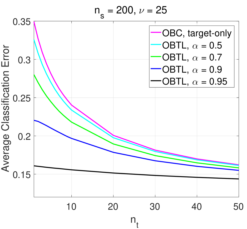
(a)

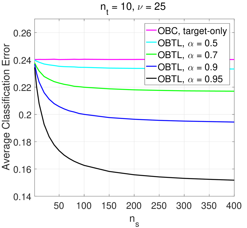
(b)

Figure 2: (a) Average classification error versus the number of target training data per class, $n_{t}$, (b) Average classification error versus the number of source training data per class, $n_{s}$.

To examine how the source data improves the classifier in target domain, we compare the performance of the OBTL classifier with the OBC designed in the target domain alone. The average classification error versus $n_{t}$ is depicted in Fig. 2a for the OBC and OBTL with different values of $\alpha$. When $\alpha$ is close to one, the performance of the OBTL classifier is much better than that of the OBC, this due to the greater relatedness between the two domains and appropriate use of the source data. This performance improvement is especially noticeable when $n_{t}$ is small, which reflects the real-world scenario. In Fig. 2a, we also observe that the errors of the OBTL classifier and OBC are converging to a similar value when $n_{t}$ gets very large, meaning that the source data are redundant when there is a large amount of target data. When $\alpha$ is larger, the error curves converge faster to the optimal error, which is the average Bayes error of the target classifier. The corresponding Bayes error averaged over $1000$ randomly generated distributions is equal to $0.122$ in this simulation setup. Recall that when $\alpha=0$, the OBTL classifier reduces to the OBC. In this particular example, the sign of $\alpha$ does not matter in the performance of the OBTL, which can be verified by (26). Hence, we can use $|\alpha|$ in all the cases.

Figure 2b depicts average classification error versus $n_{s}$ for the OBC and OBTL with different values of $\alpha$. The error of the OBC is constant for all $n_{s}$ as it does not employ the source data. The error of the OBTL classifier equals that of the OBC when $n_{s}=0$ and starts to decrease as $n_{s}$ increases. In Fig. 2b when $\alpha$ is larger, the amount of improvement is greater since the two domains are more related. Another important point in Fig. 2b is that having very large source data when the two domains are highly related can compensate the lack of target data and lead to a target classification error as small as the Bayes error in the target domain.

Figure 3 illustrates the box plots of the simulated classification errors corresponding to the $1000$ distributions randomly drawn from the prior distributions for both the OBC and OBTL with $\alpha=0.9$, which show the variability for different numbers $n_{t}$ of target data per class.

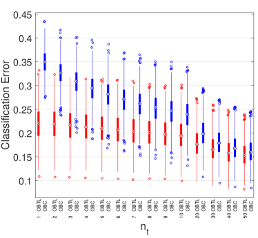
Figure 3: Box plots of $1000$ simulated classification errors for different $n_{t}$. Blue denotes the OBC and red denotes the OBTL with $\alpha=0.9$.

We investigate the sensitivity of the OBTL with respect to the hyperparameters. Fig. 4 represents the average classification error of the OBTL with respect to $|\alpha|$, where we assume that we do not know the true value $\alpha_{true}$ of the amount of relatedness between source and target domains. In Figs. 4a-4d we plot the error curves when $\alpha_{true}=0.3,0.5,0.7,0.9$, respectively. We observe several important trends in these figures. First of all, the performance gain of the OBTL towards the OBC depends heavily on the relatedness (value of $\alpha_{true}$) of source and target and the value of $\alpha$ used in the classifier. Generally speaking, there exists an $\alpha_{max}$ in $(0,1)$ such that for $|\alpha|<\alpha_{max}$, the OBTL has a performance gain towards the OBC, where the maximum gain is achieved at $|\alpha|=\alpha_{true}$ (it might not be exactly at $\alpha_{true}$ due to the Laplace approximation of the Gauss hypergeometric function). Second, the performance gain is higher when the two domains are highly related (Fig. 4d). Third, when the two domains are very related, for example, $\alpha_{true}=0.9$ in Fig. 4d, $\alpha_{max}=1$, meaning that for any $|\alpha|$, the OBTL has performance gain towards the target-only OBC. However, when the source and target domains are not related much, like Figs. 4a and 4b, $\alpha_{max}<1$, and choosing $|\alpha|$ greater than $\alpha_{max}$ leads to performance loss compared to the OBC. This means that exaggeration in the amount of relatedness between the two domains can hurt the transfer learning classifier when the two domains are not actually related, which refers to the concept of negative transfer.

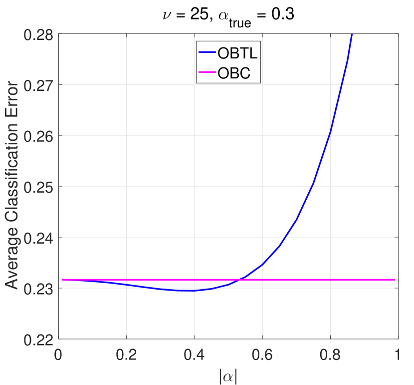
(a)

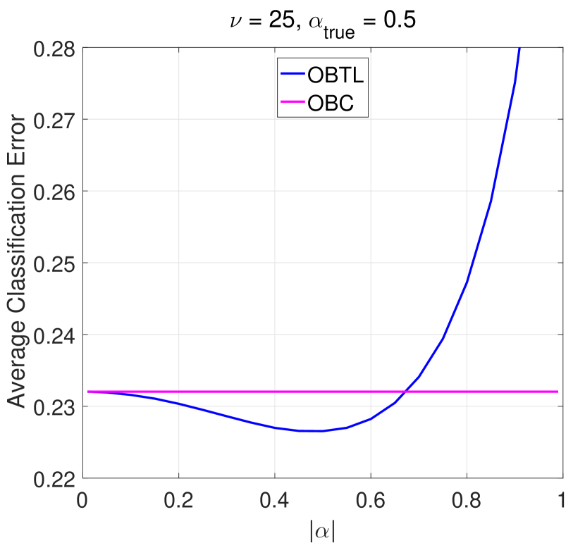
(b)

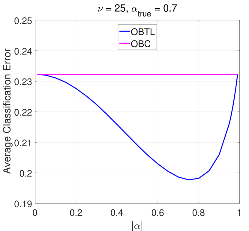
(c)

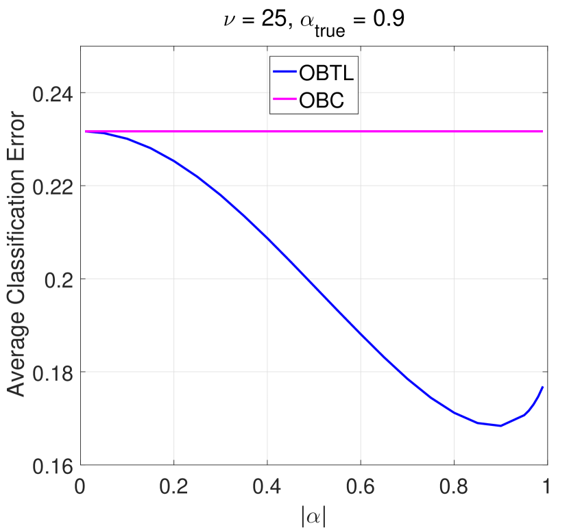
(d)

Figure 4: Average classification error vs $|\alpha|$

Figure 5 shows the errors versus $\nu$, assuming unknown true value $\nu_{true}$, for different values of $\alpha$ ($0.5$ and $0.9$) and $\nu_{true}$ ($25$ and $50$). The salient point here is that the performance of the OBTL classifier is not so sensitive to $\nu$ if it is chosen in its allowable range, that is, $\nu\geq 2d$. In Fig. 5, the error of the OBTL does not change much for $\nu\geq 2d=20$. As a result, we can choose any arbitrary $\nu\geq 2d$ in real datasets without worrying about critical performance deterioration.

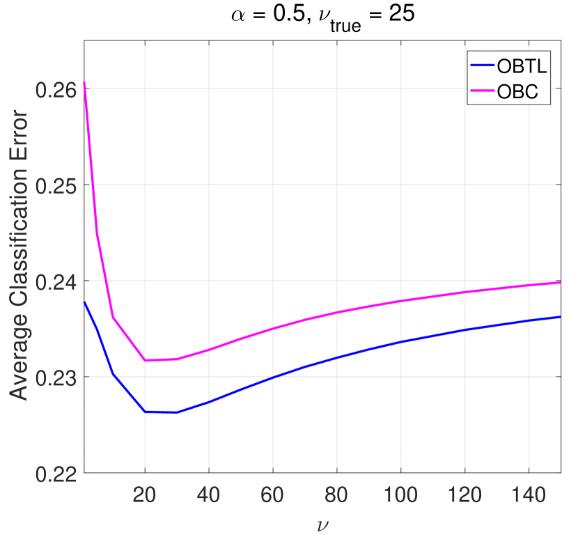
(a)

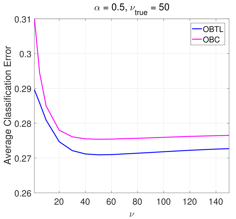
(b)

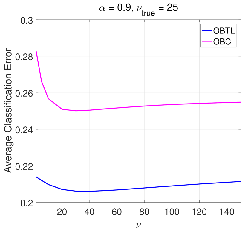
(c)

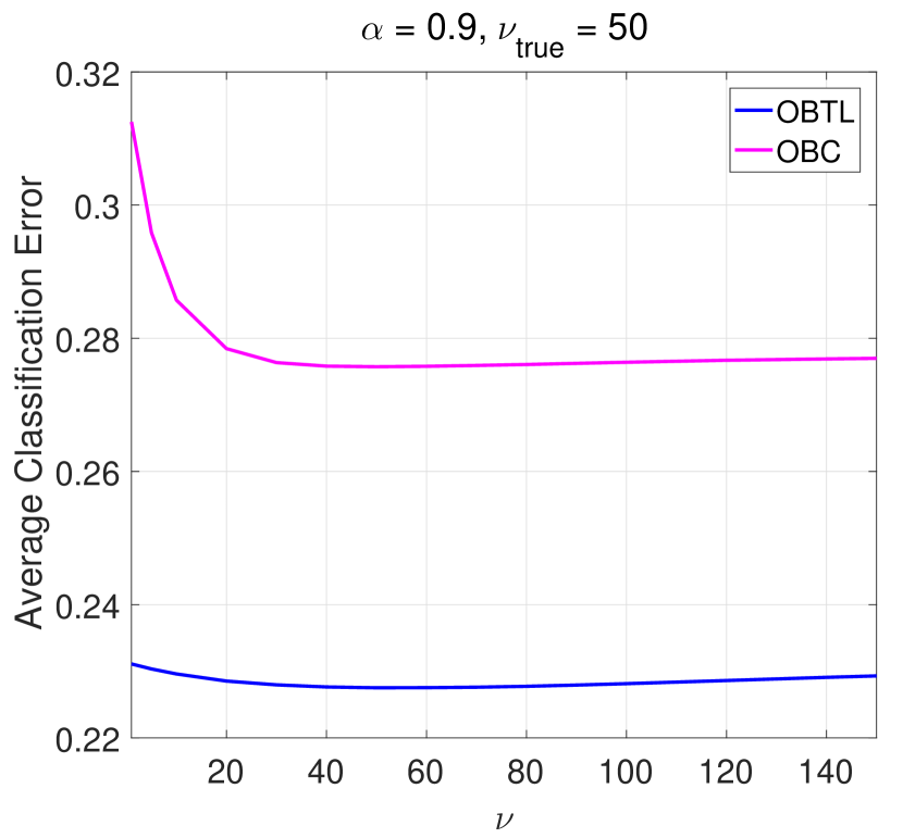
(d)

Figure 5: Average classification error vs $\nu$

Figure 6 depicts average classification error versus $\kappa_{t}$ for two different values of $\alpha$ ($0.5$ and $0.9$), where the true value of $\kappa_{t}$ is $\kappa_{true}=50$. Similar to $\nu$, if $\kappa_{t}$ is greater than a value ($20$ in Fig. 6), the performance does not change much. According to (24), it is better to choose $\kappa_{t}^{l}$ and $\kappa_{s}^{l}$ to be proportional to $n_{t}$ and $n_{s}$, respectively, since the values of updated means $\mathbf{m}_{t,n}^{l}$ and $\mathbf{m}_{s,n}^{l}$ are weighted averages of our prior knowledge about means, $\mathbf{m}_{t}^{l}$ and $\mathbf{m}_{s}^{l}$, and the sample means $\bar{\mathbf{x}}_{t}^{l}$ and $\bar{\mathbf{x}}_{s}^{l}$. Assuming that $\kappa_{t}=\beta_{t}n_{t}$ and $\kappa_{s}=\beta_{s}n_{s}$, for some $\beta_{t},\beta_{s}>0$, if we have higher confidence on our priors on means, we pick higher $\beta_{t}$ and $\beta_{s}$ (as in Fig. 6); but for the untrustworthy priors, we choose lower values for $\beta_{t}$ and $\beta_{s}$.

Sensitivity results in Figs. 4, 5, and 6 reveal that in our simulation setup the performance improvement of the OBTL depends on the value of $\alpha$ and true relatedness ($\alpha_{true}$ in this example) between the two domains and is not affected that much by the choices of other hyperparameters like $\nu$, $\kappa_{t}$, and $\kappa_{s}$. We could have a reasonable range of $\alpha$ to get improved performance but the correct estimates of relatedness or transferability are critical, which is an important future research direction (see Conclusions in Section VIII).

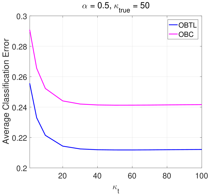
(a)

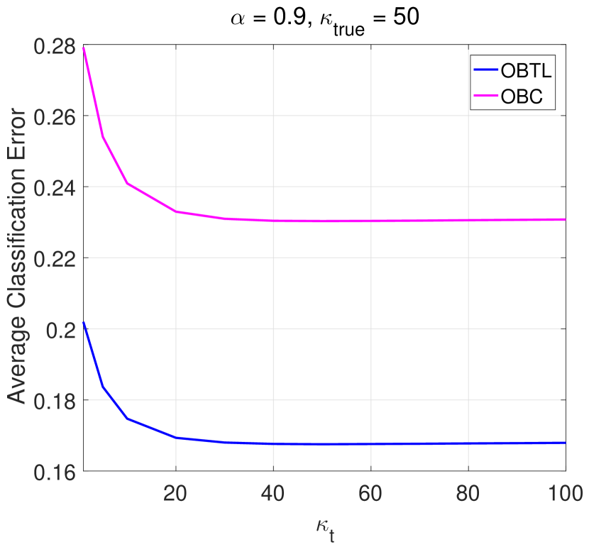
(b)

Figure 6: Average classification error vs $\kappa_{t}$

VII-B Real-world benchmark datasets

We test the OBTL classifier on Office [32] and Caltech256 [33] image datasets, which have been adopted to help benchmark different transfer learning algorithms in the literature. We have used exactly the same evaluation setup and data splits of MMDT (Max-Margin Domain Transform) [10].

Table I: Semi-supervised accuracy for different source and target domains in the Office+Caltech256 dataset using SURF features. Domain names are denoted as a: amazon, w: webcam, d: dslr, c: Caltech256. The numbers in red show the best accuracy and the numbers in blue show the second best accuracy in each column. The results of the first six methods have been adopted from [17]. Similar to [17], we have also used the evaluation setup of [10] for the OBTL.

	a $\rightarrow$ w	a $\rightarrow$ d	a $\rightarrow$ c	w $\rightarrow$ a	w $\rightarrow$ d	w $\rightarrow$ c	d $\rightarrow$ a	d $\rightarrow$ w	d $\rightarrow$ c	c $\rightarrow$ a	c $\rightarrow$ w	c $\rightarrow$ d	Mean
1-NN-t	34.5	33.6	19.7	29.5	35.9	18.9	27.1	33.4	18.6	29.2	33.5	34.1	29.0
SVM-t	63.7	57.2	32.2	46.0	56.5	29.7	45.3	62.1	32.0	45.1	60.2	56.3	48.9
HFA [9]	57.4	55.1	31.0	56.5	56.5	29.0	42.9	60.5	30.9	43.8	58.1	55.6	48.1
MMDT [10]	64.6	56. 7	36.4	47.7	67.0	32.2	46.9	74.1	34.1	49.4	63.8	56.5	52.5
CDLS [12]	68.7	60.4	35.3	51.8	60.7	33.5	50.7	68.5	34.9	50.9	66.3	59.8	53.5
ILS (1-NN) [17]	59.7	49.8	43.6	54.3	70.8	38.6	55.0	80.1	41.0	55.1	62.9	56.2	55.6
OBTL	72.4	60.2	41.5	55.0	75.0	37.4	54.4	83.2	40.3	54.8	71.1	61.5	58.9

Table II: The values of hyperparameter $\alpha$ of the OBTL used in each experiment. $n_{t}$ and $n_{s}$ are based on the data splits provided by [10].

	a $\rightarrow$ w	a $\rightarrow$ d	a $\rightarrow$ c	w $\rightarrow$ a	w $\rightarrow$ d	w $\rightarrow$ c	d $\rightarrow$ a	d $\rightarrow$ w	d $\rightarrow$ c	c $\rightarrow$ a	c $\rightarrow$ w	c $\rightarrow$ d
$n_{t}$	3	3	3	3	3	3	3	3	3	3	3	3
$n_{s}$	20	20	20	8	8	8	8	8	8	8	8	8
$\alpha$	0.6	0.75	0.99	0.9	0.99	0.99	0.9	0.99	0.99	0.85	0.5	0.75

$\bullet$ Office dataset: This dataset has images in three different domains: amazon, webcam, and dslr. The dataset contains 31 classes including the office stuff like backpack, chair, keyboard, etc. The three domains amazon, webcam, and dslr contain images from Amazon’s website, a webcam, and a digital single-lens reflex (dslr) camera, respectively, with different lighting and backgrounds. SURF [34] image features are used in all the domains, which are of dimension 800.

$\bullet$ Office + Caltech256 dataset: This dataset has $L=10$ common classes of both Office and Caltech256 datasets with the same feature dimension $d=800$. According to the data splits of [10], the numbers of training data per class in the source domain are $n_{s}=20$ for amazon and $n_{s}=8$ for the other three domains, and in the target domain $n_{t}=3$ for all the four domains. For this four-domain dataset, 20 random train-test splits have been created by [10]. We run the OBTL classifier on that 20 provided train-test splits and report the average accuracy. Note that the test data are solely from the target domains. Authors of MMDT [10] reduce the dimension to $d=20$ using PCA. We follow the same procedure for the OBTL classifier.

Following the comparison framework of [17], which used the same evaluation setup of [10], we compare the OBTL’s performance in terms of accuracy (10-class) in Table 1 with two target-only classifiers and four state-of-the-art semi-supervised transfer learning algorithms (including [17] itself). The evaluation setup is exactly the same for the OBTL and all the other six methods. As a result, we use the results of [17] for the first six methods in Table 1 and compare them with the OBTL classifier. The six methods are as follows.

$\bullet$ 1-NN-t and SVM-t: The Nearest Neighbor (1-NN) and linear SVM classifiers designed using only the target data.

$\bullet$ HFA [9]: This Heterogeneous Feature Augmentation (HFA) method learns a common latent space between source and target domains using the max-margin approach and designs a classifier in that common space.

$\bullet$ MMDT [10]: This Max-Margin Domain Transform (MMDT) method learns a transformation between the source and target domains and employs the weighted SVM for classification.

$\bullet$ CDLS [12]: This Cross-Domain Landmark Selection (CDLS) is a semi-supervised heterogeneous domain adaptation method, which derives a domain-invariant feature space for improved classification performance.

$\bullet$ ILS (1-NN) [17]: This is a recent method that learns an Invariant Latent Space (ILS) to reduce the discrepancy between the source and target domains and uses Riemannian optimization techniques to match statistical properties between samples projected into the latent space from different domains.

In Table I, we have calculated the accuracy of the OBTL classifier in 12 distinct experiments, where the source-target pairs are different (source $\rightarrow$ target) in each experiment. We have marked the best accuracy in each column with red and the second best accuracy with blue. We see that the OBTL classifier has either the best or second best accuracy in all the 12 experiments. We have written the mean accuracy of each method in the last column, which has been averaged over all the 12 different experiments. The OBTL classifier has the best mean accuracy and the ILS [17] has the second best accuracy among all the methods. We have assumed equal prior probabilities for all the classes and used (32) for the OBTL classifier.

$\bullet$ Hyperparameters of the OBTL: We assume the same values of hyperparameters for all the 10 classes in each domain, so we can drop the superscript $l$ denoting the class label. We set $\nu=10d=200$ for all the experiments. We choose $\alpha$ separately in each experiment since the relatedness between distinct pairs of domains are different. For $\mathbf{m}_{t}$ and $\mathbf{m}_{s}$, we pool all the target and source data in all the 10 classes, respectively, and use the sample means of the datasets. We fix $\beta_{t}=\beta_{s}=1$ (meaning that $\kappa_{t}=n_{t}$ and $\kappa_{s}=n_{s}$) and $k_{t}=k_{s}=1/\nu=1/200=0.005$. The mean of the Wishart precision matrix $\mathbf{\Lambda}_{z}$, for $z\in\{s,t\}$, with scale matrix $\mathbf{M}_{z}$ and $\nu$ degrees of freedom is $\nu\mathbf{M}_{z}$. Consequently, $E(\mathbf{\Lambda}_{t})=E(\mathbf{\Lambda}_{s})=I_{d}$, which is a reasonable choice, since the provided datasets of [10] have been normally standardized. Therefore, the only hyperparameter and the most important one is $\alpha$ ($\in(0,1)$), which shows the relatedness between the two domains. Figs. 7a and 7b demonstrate that the accuracy is robust for $k_{t}\in(0.005,0.02)$ and $k_{s}\in(0.005,0.02)$, respectively. Figs. 7a and 7b are corresponding to two experiments: $a\rightarrow w,\alpha=0.6$ and $w\rightarrow d,\alpha=0.99$. Figs. 7c and 7d show interesting results. We have already seen similar behavior in the synthetic data as well. In the case of $a\rightarrow w$, accuracy grows smoothly by increasing $\alpha$, reaches the maximum at $\alpha=0.6$, and decreases afterwards. This verifies the fact that the source domain $a$ cannot help the target domain $w$ that much. On the contrary, accuracy increases monotonically in Fig. 7d, in the case of $w\rightarrow d$, and the difference between accuracy for $\alpha=0.01$ and $\alpha=0.99$ is huge. This confirms that the source domain $w$ is very related to the target domain $d$ and helps it a lot. Interestingly, this coincides with the findings from the literature that the two domains $w$ and $d$ are highly related. We choose the values of $\alpha$ in each experiment which give the best accuracy. They are shown in Table II. The values of $\alpha$ in Table II also reveal the amount of relatedness between any pairs of source and target domains. For example, both $w\rightarrow d$ and $d\rightarrow w$ have high relatedness with $\alpha=0.99$, which has already been verified by other papers as well [8].

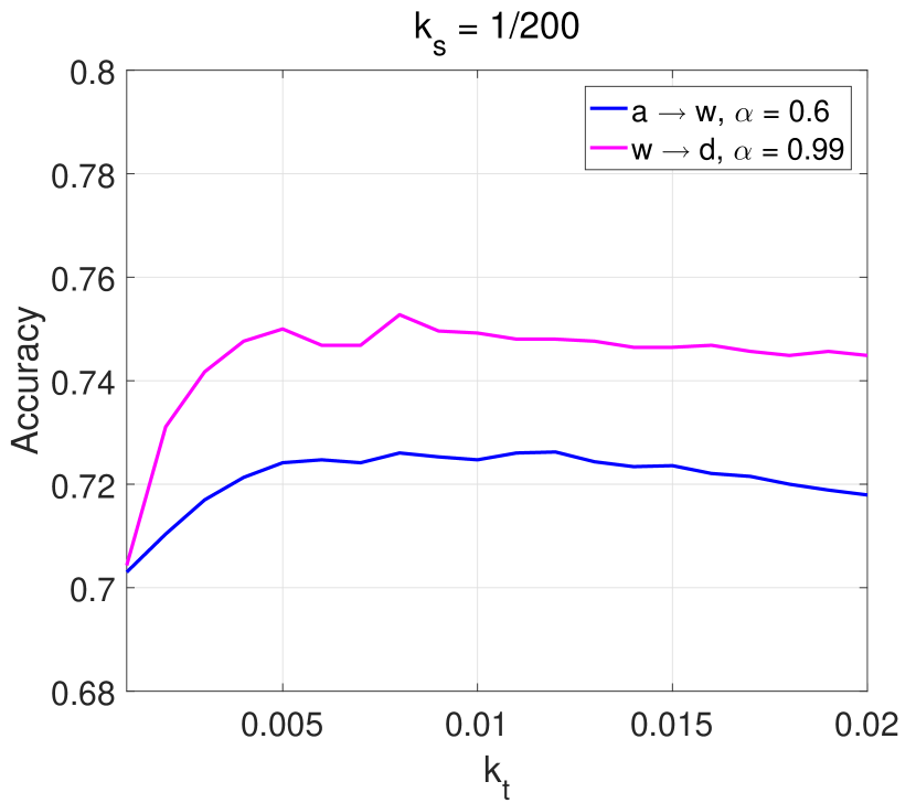
(a)

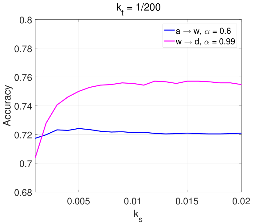
(b)

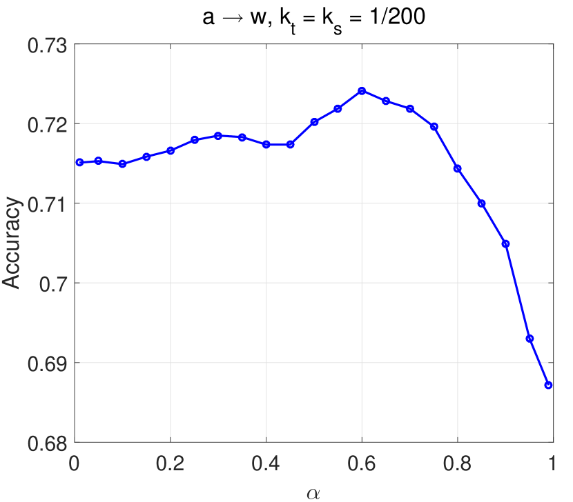
(c)

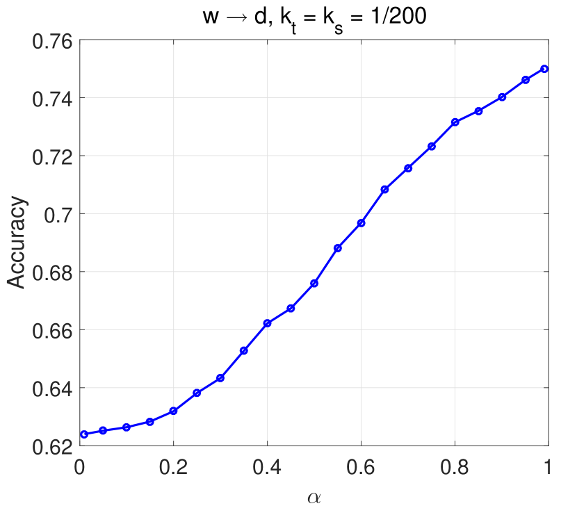
(d)

Figure 7: Accuracy in the Office+Caltech256 dataset versus: (a) $k_{t}$ when $k_{s}=1/200$ and for two experiments $a\rightarrow w,\alpha=0.6$ and $w\rightarrow d,\alpha=0.99$, (b) $k_{s}$ when $k_{t}=1/200$ and for two experiments $a\rightarrow w,\alpha=0.6$ and $w\rightarrow d,\alpha=0.99$, (c) $\alpha$ when $k_{t}=k_{s}=1/200$ and for the experiment $a\rightarrow w$, (d) $\alpha$ when $k_{t}=k_{s}=1/200$ and for the experiment $w\rightarrow d$.

VIII Conclusions And Future Work

We have constructed a Bayesian transfer learning framework to tackle the supervised transfer learning problem. The proposed Optimal Bayesian Transfer Learning (OBTL) classifier can deal with the lack of labeled data in the target domain and is optimal in this new Bayesian framework since it minimizes the expected classification error. We have obtained the closed-form posterior distribution of the target parameters and accordingly the closed-form effective class-conditional densities in the target domain to define the OBTL classifier. As the OBTL’s objective function consists of hypergeometric functions of matrix argument, we use the Laplace approximations of those functions to derive a computationally efficient and scalable OBTL classifier, while preserving its superior performance. We have compared the performance of the OBTL with its target-only version, OBC, to see how transferring from source to target domain can help. We have tested the OBTL classifier with real-world benchmark image datasets and demonstrated its excellent performance compared to other state-of-the-art domain adaption methods.

This paper considers a Gaussian model, in which we can derive closed-form solutions, as the case with the OBC. Since many practical problems cannot be approximated by a Gaussian model, an important aspect of OBC development has been the utilization of MCMC methods [35, 36]. In a forthcoming paper, we extend the OBTL setting to count data with a Negative Binomial model, in which the inference of parameters is done by MCMC. We will also apply the OBTL in dynamical systems and time series scenarios [37, 38, 39, 40].

We have only considered two domains in this paper, assuming there is only one source domain. Having seen the good performance of the OBTL classifier in two domains, in future work, we are going to apply it to the multi-source transfer learning problems, where we can benefit from the knowledge of different related sources in order to further improve the target classifier.

As in the case of the OBC, a basic engineering aspect of the OBTL is prior construction. This has been studied under different conditions in the context of the OBC: using the data from unused features to infer a prior distribution [41], deriving the prior distribution from models of the data-generating technology [35], and applying constraints based on prior knowledge to map the prior knowledge into a prior distribution via optimization [42, 43, 44]. The methods in [42, 43] are very general and have been placed into a formal mathematical structure in [44], where the prior results from an optimization involving the Kullback-Leibler (KL) divergence constrained by conditional probability statements characterizing physical knowledge, such as genetic pathways in genomic medicine. A key focus of our future work will be to extend this general framework to the OBTL, which will require a formulation that incorporates knowledge relating the source and target domains. It should be emphasized that with optimal Bayesian classification, as well as with optimal Bayesian filtering [45, 46, 47], the prior distribution is not on the operator to be designed (classifier or filter) but on the underlying scientific model (feature-label distribution, covariance matrix, or observation model) for which the operator is optimized. It is for this reason that uncertainty in the scientific model can be mapped into a prior distribution based on physical laws.

Appendix A Theorems for Zonal Polynomials and Generalized Hypergeometric Functions of Matrix Argument

Theorem 5.

[25]: Let $\mathbf{Z}$ be a complex symmetric matrix whose real part is positive-definite, and let $\mathbf{X}$ be an arbitrary complex symmetric matrix. Then

$$\int_{\mathbf{R}>0}\mathrm{etr}(-\mathbf{Z}\mathbf{R})|\mathbf{R}|^{\alpha-\frac{d+1}{2}}C_{\kappa}(\mathbf{R}\mathbf{X})d\mathbf{R}$$ (42)

$$=\Gamma_{d}(\alpha)(\alpha)_{\kappa}|\mathbf{Z}|^{-\alpha}C_{\kappa}(\mathbf{X}\mathbf{Z}^{-1}),$$

the integration being over the space of positive-definite $d\times d$ matrices, and valid for all complex numbers $\alpha$ satisfying $\mathrm{Re}(\alpha)>\frac{d-1}{2}$. $\Gamma_{d}(\alpha)$ is the multivariate gamma function defined in (8).

Theorem 6.

[48]: The zonal polynomials are invariant under orthogonal transformation. That is, for a $d\times d$ symmetric matrix $\mathbf{X}$,

$$C_{\kappa}(\mathbf{X})=C_{\kappa}(\mathbf{H}\mathbf{X}\mathbf{H}^{{}^{\prime}}),$$ (43)

where $\mathbf{H}$ is an orthogonal matrix of order $d$. If $\mathbf{R}$ is a symmetric positive-definite matrix of order $d$, then

$$C_{\kappa}(\mathbf{RX})=C_{\kappa}(\mathbf{R}^{1/2}\mathbf{X}\mathbf{R}^{1/2}).$$ (44)

As a result, if $\mathbf{R}$ is a symmetric positive-definite matrix, the hypergeometric function has the following property:

$$\leavevmode\nobreak\ {}_{p}F_{q}(a_{1},\cdots,a_{p};b_{1},\cdots,b_{q};\mathbf{RX})$$ (45)

$$=\leavevmode\nobreak\ _{p}F_{q}(a_{1},\cdots,a_{p};b_{1},\cdots,b_{q};\mathbf{R}^{1/2}\mathbf{X}\mathbf{R}^{1/2}).$$

Theorem 7.

[49]: If $\mathbf{Z}>0$ and $\mathrm{Re}(\alpha)>\frac{d-1}{2}$, and $\mathbf{X}$ is a $d\times d$ symmetric matrix, we have

$$\int_{\mathbf{R}>0}\mathrm{etr}(-\mathbf{ZR})|\mathbf{R}|^{\alpha-\frac{d+1}{2}}$$

$$\hskip 56.9055pt\times\leavevmode\nobreak\ _{p}F_{q}(a_{1},\cdots,a_{p};b_{1},\cdots,b_{q};\mathbf{RX})d\mathbf{R}$$

$$=\int_{\mathbf{R}>0}\mathrm{etr}(-\mathbf{ZR})|\mathbf{R}|^{\alpha-\frac{d+1}{2}}$$

$$\hskip 42.67912pt\times\leavevmode\nobreak\ _{p}F_{q}(a_{1},\cdots,a_{p};b_{1},\cdots,b_{q};\mathbf{R}^{1/2}\mathbf{X}\mathbf{R}^{1/2})d\mathbf{R}$$

$$=\Gamma_{d}(\alpha)|\mathbf{Z}|^{-\alpha}\leavevmode\nobreak\ _{p+1}F_{q}(a_{1},\cdots,a_{p},\alpha;b_{1},\cdots,b_{q};\mathbf{X}\mathbf{Z}^{-1}).$$

Appendix B Proof of Theorem 2

We require the following lemma.

Lemma 1.

[25] If $\mathcal{D}=\{\mathbf{x}_{1},\cdots,\mathbf{x}_{n}\}$ where $\mathbf{x}_{i}$ is a $d\times 1$ vector and $\mathbf{x}_{i}\sim\mathcal{N}(\mathbf{\mu},(\mathbf{\Lambda})^{-1})$, for $i=1,\cdots,n$, and $(\mathbf{\mu},\mathbf{\Lambda})$ has a Gaussian-Wishart prior, such that, $\mathbf{\mu}|\mathbf{\Lambda}\sim\mathcal{N}(\mathbf{m},(\kappa\mathbf{\Lambda})^{-1})$ and $\mathbf{\Lambda}\sim W_{d}(\mathbf{M},\nu)$, then the posterior of $(\mathbf{\mu},\mathbf{\Lambda})$ upon observing $\mathcal{D}$ is also a Gaussian-Wishart distribution:

$$\mathbf{\mu}|\mathbf{\Lambda},\mathcal{D} \sim\mathcal{N}(\mathbf{m}_{n},(\kappa_{n}\mathbf{\Lambda})^{-1}),$$ (46)

$$\mathbf{\Lambda}|\mathcal{D} \sim W_{d}(\mathbf{M}_{n},\nu_{n}),$$

where

$$\kappa_{n}=\kappa+n,$$ (47)

$$\nu_{n}=\nu+n,$$

$$\mathbf{m}_{n}=\frac{\kappa\mathbf{m}+n\bar{\mathbf{x}}}{\kappa+n},$$

$$\mathbf{M}_{n}^{-1}=\mathbf{M}^{-1}+\mathbf{S}+\frac{\kappa n}{\kappa+n}(\mathbf{m}-\bar{\mathbf{x}})(\mathbf{m}-\bar{\mathbf{x}})^{{}^{\prime}},$$

depending on the sample mean and covariance matrix

$$\bar{\mathbf{x}}=\frac{1}{n}\sum_{i=1}^{n}\mathbf{x}_{i},$$ (48)

$$\mathbf{S}=\sum_{i=1}^{n}(\mathbf{x}_{i}-\bar{\mathbf{x}})(\mathbf{x}_{i}-\bar{\mathbf{x}})^{{}^{\prime}}.$$

We now provide the proof. From (3), for each domain $z\in\{s,t\}$,

$$p(\mathcal{D}_{z}^{l}|\mathbf{\mu}_{z}^{l},\mathbf{\Lambda}_{z}^{l})=(2\pi)^{-\frac{dn_{z}^{l}}{2}}\leavevmode\nobreak\ \left|\mathbf{\Lambda}_{z}^{l}\right|^{\frac{n_{z}^{l}}{2}}\exp\left(-\frac{1}{2}\mathbf{Q}_{z}^{l}\right),$$ (49)

where $\mathbf{Q}_{z}^{l}=\sum_{i=1}^{n_{z}^{l}}\left(\mathbf{x}_{z,i}^{l}-\mathbf{\mu}_{z}^{l}\right)^{{}^{\prime}}\mathbf{\Lambda}_{z}^{l}\left(\mathbf{x}_{z,i}^{l}-\mathbf{\mu}_{z}^{l}\right)$. Moreover, from (6), for each domain $z\in\{s,t\}$,

$$p\left(\mathbf{\mu}_{z}^{l}|\mathbf{\Lambda}_{z}^{l}\right)=(2\pi)^{-\frac{d}{2}}\left(\kappa_{z}^{l}\right)^{\frac{d}{2}}\left|\mathbf{\Lambda}_{z}^{l}\right|^{\frac{1}{2}}\hskip 56.9055pt$$

$$\times\exp\left(-\frac{\kappa_{z}^{l}}{2}\left(\mathbf{\mu}_{z}^{l}-\mathbf{m}_{z}^{l}\right)^{{}^{\prime}}\mathbf{\Lambda}_{z}^{l}\left(\mathbf{\mu}_{z}^{l}-\mathbf{m}_{z}^{l}\right)\right).$$ (50)

From (13), (21), (49), and (50),

$$p(\mathbf{\mu}_{t}^{l},\mathbf{\Lambda}_{t}^{l}|\mathcal{D}_{t}^{l},\mathcal{D}_{s}^{l})\propto\left|\mathbf{\Lambda}_{t}^{l}\right|^{\frac{n_{t}^{l}}{2}}\exp\left(-\frac{1}{2}\mathbf{Q}_{t}^{l}\right)\left|\mathbf{\Lambda}_{t}^{l}\right|^{\frac{1}{2}}$$ (51)

$$\times\exp\left(-\frac{\kappa_{t}^{l}}{2}\left(\mathbf{\mu}_{t}^{l}-\mathbf{m}_{t}^{l}\right)^{{}^{\prime}}\mathbf{\Lambda}_{t}^{l}\left(\mathbf{\mu}_{t}^{l}-\mathbf{m}_{t}^{l}\right)\right)$$

$$\times\left|\mathbf{\Lambda}_{t}^{l}\right|^{\frac{\nu^{l}-d-1}{2}}\mathrm{etr}\left(-\frac{1}{2}\left({\left(\mathbf{M}_{t}^{l}\right)}^{-1}+{\mathbf{F}^{l}}^{{}^{\prime}}\mathbf{C}^{l}\mathbf{F}^{l}\right)\mathbf{\Lambda}_{t}^{l}\right)$$

$$\times\int_{\mathbf{\mu}_{s}^{l},\mathbf{\Lambda}_{s}^{l}}\left\{\left|\mathbf{\Lambda}_{s}^{l}\right|^{\frac{n_{s}^{l}}{2}}\exp\left(-\frac{1}{2}\mathbf{Q}_{s}^{l}\right)\left|\mathbf{\Lambda}_{s}^{l}\right|^{\frac{1}{2}}\right.$$

$$\times\exp\left(-\frac{\kappa_{s}^{l}}{2}\left(\mathbf{\mu}_{s}^{l}-\mathbf{m}_{s}^{l}\right)^{{}^{\prime}}\mathbf{\Lambda}_{s}^{l}\left(\mu_{s}^{l}-\mathbf{m}_{s}^{l}\right)\right)$$

$$\times\left|\mathbf{\Lambda}_{s}^{l}\right|^{\frac{\nu^{l}-d-1}{2}}\mathrm{etr}\left(-\frac{1}{2}{\left(\mathbf{C}^{l}\right)}^{-1}\mathbf{\Lambda}_{s}^{l}\right)$$

$$\left.\times\leavevmode\nobreak\ _{0}F_{1}\left(\frac{\nu^{l}}{2};\frac{1}{4}{\mathbf{\Lambda}_{s}^{l}}^{\frac{1}{2}}\mathbf{F}^{l}\mathbf{\Lambda}_{t}^{l}{\mathbf{F}^{l}}^{{}^{\prime}}{\mathbf{\Lambda}_{s}^{l}}^{\frac{1}{2}}\right)\right\}d\mathbf{\mu}_{s}^{l}d\mathbf{\Lambda}_{s}^{l}.$$

Using Lemma 1 we can simplify (51) as

$$p(\mathbf{\mu}_{t}^{l},\mathbf{\Lambda}_{t}^{l}|\mathcal{D}_{t}^{l},\mathcal{D}_{s}^{l})$$ (52)

$$\propto\left|\mathbf{\Lambda}_{t}^{l}\right|^{\frac{1}{2}}\exp\left(-\frac{\kappa_{t,n}^{l}}{2}\left(\mathbf{\mu}_{t}^{l}-\mathbf{m}_{t,n}^{l}\right)^{{}^{\prime}}\mathbf{\Lambda}_{t}^{l}\left(\mathbf{\mu}_{t}^{l}-\mathbf{m}_{t,n}^{l}\right)\right)$$

$$\times\left|\mathbf{\Lambda}_{t}^{l}\right|^{\frac{\nu^{l}+n_{t}^{l}-d-1}{2}}\mathrm{etr}\left(-\frac{1}{2}{\left(\mathbf{T}_{t}^{l}\right)}^{-1}\mathbf{\Lambda}_{t}^{l}\right)$$

$$\int_{\mathbf{\mu}_{s}^{l},\mathbf{\Lambda}_{s}^{l}}\left\{\left|\mathbf{\Lambda}_{s}^{l}\right|^{\frac{1}{2}}\exp\left(-\frac{\kappa_{s,n}^{l}}{2}\left(\mathbf{\mu}_{s}^{l}-\mathbf{m}_{s,n}^{l}\right)^{{}^{\prime}}\mathbf{\Lambda}_{s}^{l}\left(\mathbf{\mu}_{s}^{l}-\mathbf{m}_{s,n}^{l}\right)\right)\right.$$

$$\times\left|\mathbf{\Lambda}_{s}^{l}\right|^{\frac{\nu^{l}+n_{s}^{l}-d-1}{2}}\mathrm{etr}\left(-\frac{1}{2}{\left(\mathbf{T}_{s}^{l}\right)}^{-1}\mathbf{\Lambda}_{s}^{l}\right)$$

$$\left.\times\leavevmode\nobreak\ _{0}F_{1}\left(\frac{\nu^{l}}{2};\frac{1}{4}{\mathbf{\Lambda}_{s}^{l}}^{\frac{1}{2}}\mathbf{F}^{l}\mathbf{\Lambda}_{t}^{l}{\mathbf{F}^{l}}^{{}^{\prime}}{\mathbf{\Lambda}_{s}^{l}}^{\frac{1}{2}}\right)\right\}d\mathbf{\mu}_{s}^{l}d\mathbf{\Lambda}_{s}^{l},$$

where

$$\kappa_{t,n}^{l}=\kappa_{t}^{l}+n_{t}^{l},\hskip 42.67912pt\kappa_{s,n}^{l}=\kappa_{s}^{l}+n_{s}^{l},$$ (53)

$$\mathbf{m}_{t,n}^{l}=\frac{\kappa_{t}^{l}\mathbf{m}_{t}^{l}+n_{t}^{l}\bar{\mathbf{x}}_{t}^{l}}{\kappa_{t}^{l}+n_{t}^{l}},\leavevmode\nobreak\ \leavevmode\nobreak\ \leavevmode\nobreak\ \leavevmode\nobreak\ \leavevmode\nobreak\ \mathbf{m}_{s,n}^{l}=\frac{\kappa_{s}^{l}\mathbf{m}_{s}^{l}+n_{s}^{l}\bar{\mathbf{x}}_{s}^{l}}{\kappa_{s}^{l}+n_{s}^{l}},$$

$${\left(\mathbf{T}_{t}^{l}\right)}^{-1}={\left(\mathbf{M}_{t}^{l}\right)}^{-1}+{\mathbf{F}^{l}}^{{}^{\prime}}\mathbf{C}^{l}\mathbf{F}^{l}+\mathbf{S}_{t}^{l}$$

$$\hskip 56.9055pt+\frac{\kappa_{t}^{l}n_{t}^{l}}{\kappa_{t}^{l}+n_{t}^{l}}(\mathbf{m}_{t}^{l}-\bar{\mathbf{x}}_{t}^{l})(\mathbf{m}_{t}^{l}-\bar{\mathbf{x}}_{t}^{l})^{{}^{\prime}},$$

$${\left(\mathbf{T}_{s}^{l}\right)}^{-1}={\left(\mathbf{C}^{l}\right)}^{-1}+\mathbf{S}_{s}^{l}+\frac{\kappa_{s}^{l}n_{s}^{l}}{\kappa_{s}^{l}+n_{s}^{l}}(\mathbf{m}_{s}^{l}-\bar{\mathbf{x}}_{s}^{l})(\mathbf{m}_{s}^{l}-\bar{\mathbf{x}}_{s}^{l})^{{}^{\prime}},$$

with sample means and covariances for $z\in\{s,t\}$ as

$$\bar{\mathbf{x}}_{z}^{l}=\frac{1}{n_{z}^{l}}\sum_{i=1}^{n_{z}^{l}}\mathbf{x}_{z,i}^{l},\leavevmode\nobreak\ \leavevmode\nobreak\ \leavevmode\nobreak\ \mathbf{S}_{z}^{l}=\sum_{i=1}^{n_{z}^{l}}\left(\mathbf{x}_{z,i}^{l}-\bar{\mathbf{x}}_{z}^{l}\right)\left(\mathbf{x}_{z,i}^{l}-\bar{\mathbf{x}}_{z}^{l}\right)^{{}^{\prime}}.$$

Using the equation

$$\int_{\mathbf{x}}\exp\left(-\frac{1}{2}(\mathbf{x}-\mathbf{\mu})^{{}^{\prime}}\mathbf{\Lambda}(\mathbf{x}-\mathbf{\mu})\right)d\mathbf{x}=(2\pi)^{\frac{d}{2}}|\mathbf{\Lambda}|^{-\frac{1}{2}},$$ (54)

and integrating out $\mathbf{\mu}_{s}^{l}$ in (52) yields

$$p(\mathbf{\mu}_{t}^{l},\mathbf{\Lambda}_{t}^{l}|\mathcal{D}_{t}^{l},\mathcal{D}_{s}^{l})$$ (55)

$$\propto\left|\mathbf{\Lambda}_{t}^{l}\right|^{\frac{1}{2}}\exp\left(-\frac{\kappa_{t,n}^{l}}{2}\left(\mathbf{\mu}_{t}^{l}-\mathbf{m}_{t,n}^{l}\right)^{{}^{\prime}}\mathbf{\Lambda}_{t}^{l}\left(\mathbf{\mu}_{t}^{l}-\mathbf{m}_{t,n}^{l}\right)\right)$$

$$\times\left|\mathbf{\Lambda}_{t}^{l}\right|^{\frac{\nu^{l}+n_{t}^{l}-d-1}{2}}\mathrm{etr}\left(-\frac{1}{2}{\left(\mathbf{T}_{t}^{l}\right)}^{-1}\mathbf{\Lambda}_{t}^{l}\right)$$

$$\times\int_{\mathbf{\Lambda}_{s}^{l}}\left\{\left|\mathbf{\Lambda}_{s}^{l}\right|^{\frac{\nu^{l}+n_{s}^{l}-d-1}{2}}\mathrm{etr}\left(-\frac{1}{2}{\left(\mathbf{T}_{s}^{l}\right)}^{-1}\mathbf{\Lambda}_{s}^{l}\right)\right.$$

$$\hskip 42.67912pt\times\left.{}_{0}F_{1}\left(\frac{\nu^{l}}{2};\frac{1}{4}{\mathbf{\Lambda}_{s}^{l}}^{\frac{1}{2}}\mathbf{F}^{l}\mathbf{\Lambda}_{t}^{l}{\mathbf{F}^{l}}^{{}^{\prime}}{\mathbf{\Lambda}_{s}^{l}}^{\frac{1}{2}}\right)\right\}d\mathbf{\Lambda}_{s}^{l}.$$

The integral, $I$, in (55) can be done using Theorem 7 as

$$I=\Gamma_{d}\left(\frac{\nu^{l}+n_{s}^{l}}{2}\right)$$ (56)

$$\times\left|2\mathbf{T}_{s}^{l}\right|^{\frac{\nu^{l}+n_{s}^{l}}{2}}\leavevmode\nobreak\ _{1}F_{1}\left(\frac{\nu^{l}+n_{s}^{l}}{2};\frac{\nu^{l}}{2};\frac{1}{2}\mathbf{F}^{l}\mathbf{\Lambda}_{t}^{l}{\mathbf{F}^{l}}^{{}^{\prime}}\mathbf{T}_{s}^{l}\right),$$

where ${}_{1}F_{1}(a;b;\mathbf{X})$ is the Confluent hypergeometric function with the matrix argument $\mathbf{X}$. As a result, (55) becomes

$$p(\mathbf{\mu}_{t}^{l},\mathbf{\Lambda}_{t}^{l}|\mathcal{D}_{t}^{l},\mathcal{D}_{s}^{l})=$$ (57)

$$A^{l}\left|\mathbf{\Lambda}_{t}^{l}\right|^{\frac{1}{2}}\exp\left(-\frac{\kappa_{t,n}^{l}}{2}\left(\mathbf{\mu}_{t}^{l}-\mathbf{m}_{t,n}^{l}\right)^{{}^{\prime}}\mathbf{\Lambda}_{t}^{l}\left(\mathbf{\mu}_{t}^{l}-\mathbf{m}_{t,n}^{l}\right)\right)$$

$$\times\left|\mathbf{\Lambda}_{t}^{l}\right|^{\frac{\nu^{l}+n_{t}^{l}-d-1}{2}}\mathrm{etr}\left(-\frac{1}{2}{\left(\mathbf{T}_{t}^{l}\right)}^{-1}\mathbf{\Lambda}_{t}^{l}\right)$$

$$\times\leavevmode\nobreak\ _{1}F_{1}\left(\frac{\nu^{l}+n_{s}^{l}}{2};\frac{\nu^{l}}{2};\frac{1}{2}\mathbf{F}^{l}\mathbf{\Lambda}_{t}^{l}{\mathbf{F}^{l}}^{{}^{\prime}}\mathbf{T}_{s}^{l}\right),$$

where the constant of proportionality, $A^{l}$, makes the integration of the posterior $p(\mathbf{\mu}_{t}^{l},\mathbf{\Lambda}_{t}^{l}|\mathcal{D}_{t}^{l},\mathcal{D}_{s}^{l})$ with respect to $\mathbf{\mu}_{t}^{l}$ and $\mathbf{\Lambda}_{t}^{l}$ equal to one. Hence,

$${\left(A^{l}\right)}^{-1}=\int_{\mathbf{\Lambda}_{t}^{l}}\left|\mathbf{\Lambda}_{t}^{l}\right|^{\frac{\nu^{l}+n_{t}^{l}-d-1}{2}}\mathrm{etr}\left(-\frac{1}{2}{\left(\mathbf{T}_{t}^{l}\right)}^{-1}\mathbf{\Lambda}_{t}^{l}\right)\left|\mathbf{\Lambda}_{t}^{l}\right|^{\frac{1}{2}}$$ (58)

$$\times\int_{\mathbf{\mu}_{t}^{l}}\exp\left(-\frac{\kappa_{t,n}^{l}}{2}\left(\mathbf{\mu}_{t}^{l}-\mathbf{m}_{t,n}^{l}\right)^{{}^{\prime}}\mathbf{\Lambda}_{t}^{l}\left(\mathbf{\mu}_{t}^{l}-\mathbf{m}_{t,n}^{l}\right)\right)d\mathbf{\mu}_{t}^{l}$$

$$\times_{1}F_{1}\left(\frac{\nu^{l}+n_{s}^{l}}{2};\frac{\nu^{l}}{2};\frac{1}{2}\mathbf{F}^{l}\mathbf{\Lambda}_{t}^{l}{\mathbf{F}^{l}}^{{}^{\prime}}\mathbf{T}_{s}^{l}\right)d\mathbf{\Lambda}_{t}^{l}.$$

Using (54), the inner integral equals to $(2\pi)^{\frac{d}{2}}|\kappa_{t,n}^{l}\mathbf{\Lambda}_{t}^{l}|^{-\frac{1}{2}}=\left(\frac{2\pi}{\kappa_{t,n}^{l}}\right)^{\frac{d}{2}}|\mathbf{\Lambda}_{t}^{l}|^{-\frac{1}{2}}$. Hence,

$${\left(A^{l}\right)}^{-1}=\left(\frac{2\pi}{\kappa_{t,n}^{l}}\right)^{\frac{d}{2}}\int_{\mathbf{\Lambda}_{t}^{l}}\left|\mathbf{\Lambda}_{t}^{l}\right|^{\frac{\nu^{l}+n_{t}^{l}-d-1}{2}}\mathrm{etr}\left(-\frac{1}{2}{\left(\mathbf{T}_{t}^{l}\right)}^{-1}\mathbf{\Lambda}_{t}^{l}\right)$$ (59)

$$\times\leavevmode\nobreak\ _{1}F_{1}\left(\frac{\nu^{l}+n_{s}^{l}}{2};\frac{\nu^{l}}{2};\frac{1}{2}\mathbf{F}^{l}\mathbf{\Lambda}_{t}^{l}{\mathbf{F}^{l}}^{{}^{\prime}}\mathbf{T}_{s}^{l}\right)d\mathbf{\Lambda}_{t}^{l}.$$

With the variable change $\Omega=\mathbf{F}^{l}\mathbf{\Lambda}_{t}^{l}{\mathbf{F}^{l}}^{{}^{\prime}}$, we have $d\Omega=|\mathbf{F}^{l}|^{d+1}d\mathbf{\Lambda}_{t}^{l}$ and $\mathbf{\Lambda}_{t}^{l}={\left(\mathbf{F}^{l}\right)}^{-1}\Omega\left({\mathbf{F}^{l}}^{{}^{\prime}}\right)^{-1}$. Since $\mathrm{tr}(\mathbf{ABCD})=\mathrm{tr}(\mathbf{BCDA})=\mathrm{tr}(\mathbf{CDAB})=\mathrm{tr}(\mathbf{DABC})$ and $|\mathbf{ABC}|=|\mathbf{A}||\mathbf{B}||\mathbf{C}|$, $A^{l}$ can be derived as

$${\left(A^{l}\right)}^{-1}=\left(\frac{2\pi}{\kappa_{t,n}^{l}}\right)^{\frac{d}{2}}|\mathbf{F}^{l}|^{-\left(\nu^{l}+n_{t}^{l}\right)}\int_{\Omega}\left\{|\Omega|^{\frac{\nu^{l}+n_{t}^{l}-d-1}{2}}\right.$$ (60)

$$\hskip 14.22636pt\times\mathrm{etr}\left(-\frac{1}{2}{\left({\mathbf{F}^{l}}^{{}^{\prime}}\right)}^{-1}{\left(\mathbf{T}_{t}^{l}\right)}^{-1}{\mathbf{F}^{l}}^{-1}\Omega\right)$$

$$\left.\hskip 14.22636pt\times\leavevmode\nobreak\ _{1}F_{1}\left(\frac{\nu^{l}+n_{s}^{l}}{2};\frac{\nu^{l}}{2};\frac{1}{2}\Omega\mathbf{T}_{s}^{l}\right)\right\}d\Omega$$

$$=\left(\frac{2\pi}{\kappa_{t,n}^{l}}\right)^{\frac{d}{2}}2^{\frac{d\left(\nu^{l}+n_{t}^{l}\right)}{2}}\Gamma_{d}\left(\frac{\nu^{l}+n_{t}^{l}}{2}\right)\left|\mathbf{T}_{t}^{l}\right|^{\frac{\nu^{l}+n_{t}^{l}}{2}}$$

$$\leavevmode\nobreak\ \leavevmode\nobreak\ \leavevmode\nobreak\ \leavevmode\nobreak\ \leavevmode\nobreak\ \leavevmode\nobreak\ \times\leavevmode\nobreak\ _{2}F_{1}\left(\frac{\nu^{l}+n_{s}^{l}}{2},\frac{\nu^{l}+n_{t}^{l}}{2};\frac{\nu^{l}}{2};\mathbf{T}_{s}^{l}\mathbf{F}^{l}\mathbf{T}_{t}^{l}{\mathbf{F}^{l}}^{{}^{\prime}}\right),$$

where the second equality follows from Theorem 7, and ${}_{2}F_{1}(a,b;c;\mathbf{X})$ is the Gauss hypergeometric function with the matrix argument $\mathbf{X}$. As such, we have derived the closed-form posterior distribution of the target parameters $(\mathbf{\mu}_{t}^{l},\mathbf{\Lambda}_{t}^{l})$ in (22), where ${A^{l}}$ is given by (23).

Appendix C Proof of Theorem 3

The likelihood $p(\mathbf{x}|\mathbf{\mu}_{t}^{l},\mathbf{\Lambda}_{t}^{l})$ and posterior $p(\mathbf{\mu}_{t}^{l},\mathbf{\Lambda}_{t}^{l}|\mathcal{D}_{t}^{l},\mathcal{D}_{s}^{l})$ are given in (3) and (22), respectively. Hence,

$$p(\mathbf{x}|l)=(2\pi)^{-\frac{d}{2}}A^{l}\int_{\mathbf{\mu}_{t}^{l},\mathbf{\Lambda}_{t}^{l}}\left\{|\mathbf{\Lambda}_{t}^{l}|^{\frac{1}{2}}\right.$$ (61)

$$\times\exp\left(-\frac{1}{2}\left(\mathbf{x}-\mathbf{\mu}_{t}^{l}\right)^{{}^{\prime}}\mathbf{\Lambda}_{t}^{l}\left(\mathbf{x}-\mathbf{\mu}_{t}^{l}\right)\right)$$

$$\times\left|\mathbf{\Lambda}_{t}^{l}\right|^{\frac{1}{2}}\exp\left(-\frac{\kappa_{t,n}^{l}}{2}\left(\mathbf{\mu}_{t}^{l}-\mathbf{m}_{t,n}^{l}\right)^{{}^{\prime}}\mathbf{\Lambda}_{t}^{l}\left(\mathbf{\mu}_{t}^{l}-\mathbf{m}_{t,n}^{l}\right)\right)$$

$$\times\left|\mathbf{\Lambda}_{t}^{l}\right|^{\frac{\nu^{l}+n_{t}^{l}-d-1}{2}}\mathrm{etr}\left(-\frac{1}{2}{\left(\mathbf{T}_{t}^{l}\right)}^{-1}\mathbf{\Lambda}_{t}^{l}\right)$$

$$\left.\times\leavevmode\nobreak\ _{1}F_{1}\left(\frac{\nu^{l}+n_{s}^{l}}{2};\frac{\nu^{l}}{2};\frac{1}{2}\mathbf{F}^{l}\mathbf{\Lambda}_{t}^{l}{\mathbf{F}^{l}}^{{}^{\prime}}\mathbf{T}_{s}^{l}\right)\right\}d\mathbf{\mu}_{t}^{l}d\mathbf{\Lambda}_{t}^{l}.$$

Similarly, we can simplify (61) as

$$p(\mathbf{x}|l)=(2\pi)^{-\frac{d}{2}}A^{l}\int_{\mathbf{\mu}_{t}^{l},\mathbf{\Lambda}_{t}^{l}}\left\{|\mathbf{\Lambda}_{t}^{l}|^{\frac{1}{2}}\right.$$ (62)

$$\times\exp\left(-\frac{\kappa_{\mathbf{x}}^{l}}{2}\left(\mathbf{\mu}_{t}^{l}-\mathbf{m}_{\mathbf{x}}^{l}\right)^{{}^{\prime}}\mathbf{\Lambda}_{t}^{l}\left(\mathbf{\mu}_{t}^{l}-\mathbf{m}_{\mathbf{x}}^{l}\right)\right)$$

$$\times\left|\mathbf{\Lambda}_{t}^{l}\right|^{\frac{\nu^{l}+n_{t}^{l}+1-d-1}{2}}\mathrm{etr}\left(-\frac{1}{2}{\left(\mathbf{T}_{\mathbf{x}}^{l}\right)}^{-1}\mathbf{\Lambda}_{t}^{l}\right)$$

$$\left.\times\leavevmode\nobreak\ _{1}F_{1}\left(\frac{\nu^{l}+n_{s}^{l}}{2};\frac{\nu^{l}}{2};\frac{1}{2}\mathbf{F}^{l}\mathbf{\Lambda}_{t}^{l}{\mathbf{F}^{l}}^{{}^{\prime}}\mathbf{T}_{s}^{l}\right)\right\}d\mathbf{\mu}_{t}^{l}d\mathbf{\Lambda}_{t}^{l},$$

where

$$\kappa_{\mathbf{x}}^{l}=\kappa_{t,n}^{l}+1=\kappa_{t}^{l}+n_{t}^{l}+1,\leavevmode\nobreak\ \leavevmode\nobreak\ \leavevmode\nobreak\ \leavevmode\nobreak\ \leavevmode\nobreak\ \mathbf{m}_{\mathbf{x}}^{l}=\frac{\kappa_{t,n}^{l}\mathbf{m}_{t,n}^{l}+\mathbf{x}}{\kappa_{t,n}+1},$$ (63)

$${\left(\mathbf{T}_{\mathbf{x}}^{l}\right)}^{-1}={\left(\mathbf{T}_{t}^{l}\right)}^{-1}+\frac{\kappa_{t,n}^{l}}{\kappa_{t,n}^{l}+1}\left(\mathbf{m}_{t,n}^{l}-\mathbf{x}\right)\left(\mathbf{m}_{t,n}^{l}-\mathbf{x}\right)^{{}^{\prime}}.$$

The integration in (62) is similar to the one in (58). As a result, using (23),

$$p(\mathbf{x}|l)=(2\pi)^{-\frac{d}{2}}A^{l}\left(\frac{2\pi}{\kappa_{\mathbf{x}}^{l}}\right)^{\frac{d}{2}}2^{\frac{d\left(\nu^{l}+n_{t}^{l}+1\right)}{2}}\Gamma_{d}\left(\frac{\nu^{l}+n_{t}^{l}+1}{2}\right)$$ (64)

$$\left|\mathbf{T}_{\mathbf{x}}^{l}\right|^{\frac{\nu^{l}+n_{t}^{l}+1}{2}}\leavevmode\nobreak\ _{2}F_{1}\left(\frac{\nu^{l}+n_{s}^{l}}{2},\frac{\nu^{l}+n_{t}^{l}+1}{2};\frac{\nu^{l}}{2};\mathbf{T}_{s}^{l}\mathbf{F}^{l}\mathbf{T}_{\mathbf{x}}^{l}{\mathbf{F}^{l}}^{{}^{\prime}}\right).$$

By replacing the value of $A^{l}$, we have the effective class-conditional density. We denote $O_{\mathrm{OBTL}}(\mathbf{x}|l)=p(\mathbf{x}|l)$, since it is the objective function for the OBTL classifier. As such,

$$O_{\mathrm{OBTL}}(\mathbf{x}|l)=\pi^{-\frac{d}{2}}\left(\frac{\kappa_{t,n}^{l}}{\kappa_{\mathbf{x}}^{l}}\right)^{\frac{d}{2}}\Gamma_{d}\left(\frac{\nu^{l}+n_{t}^{l}+1}{2}\right)$$ (65)

$$\times\Gamma_{d}^{-1}\left(\frac{\nu^{l}+n_{t}^{l}}{2}\right)\left|\mathbf{T}_{\mathbf{x}}^{l}\right|^{\frac{\nu^{l}+n_{t}^{l}+1}{2}}\left|\mathbf{T}_{t}^{l}\right|^{-\frac{\nu^{l}+n_{t}^{l}}{2}}$$

$$\times\leavevmode\nobreak\ _{2}F_{1}\left(\frac{\nu^{l}+n_{s}^{l}}{2},\frac{\nu^{l}+n_{t}^{l}+1}{2};\frac{\nu^{l}}{2};\mathbf{T}_{s}^{l}\mathbf{F}^{l}\mathbf{T}_{\mathbf{x}}^{l}{\mathbf{F}^{l}}^{{}^{\prime}}\right)$$

$$\times\leavevmode\nobreak\ _{2}F_{1}^{-1}\left(\frac{\nu^{l}+n_{s}^{l}}{2},\frac{\nu^{l}+n_{t}^{l}}{2};\frac{\nu^{l}}{2};\mathbf{T}_{s}^{l}\mathbf{F}^{l}\mathbf{T}_{t}^{l}{\mathbf{F}^{l}}^{{}^{\prime}}\right).$$

Appendix D Laplace Approximation of the Gauss Hypergeometric Function of Matrix Argument

The Gauss hypergeomeric function has the following integral representation:

$$\leavevmode\nobreak\ {}_{2}F_{1}(a,b;c;\mathbf{X})=B_{d}^{-1}(a,c-a)$$ (66)

$$\times\int_{0_{d}<\mathbf{Y}<\mathbf{I}_{d}}|\mathbf{Y}|^{a-\frac{d+1}{2}}|\mathbf{I}_{d}-\mathbf{Y}|^{c-a-\frac{d+1}{2}}|\mathbf{I}_{d}-\mathbf{X}\mathbf{Y}|^{-b}d\mathbf{Y},$$

which is valid under the following conditions: $\mathbf{X}\in\mathbf{C}^{d\times d}$ is symmetric and satisfies $\mathrm{Re}(\mathbf{X})<\mathbf{I}_{d}$, $\mathrm{Re}(a)>\frac{d-1}{2}$, and $\mathrm{Re}(c-a)>\frac{d-1}{2}$. $B_{d}(\alpha,\beta)$ is the multivariate beta function

$$B_{d}(\alpha,\beta)=\frac{\Gamma_{d}(\alpha)\Gamma_{d}(\beta)}{\Gamma_{d}(\alpha+\beta)},$$ (67)

where $\Gamma_{d}(\alpha)$ is the multivariate gamma function defined in (8). The Laplace approximation is one common solution to approximate the integral

$$I=\int_{y\in D}h(y)\exp(-\lambda g(y))dy,$$ (68)

where $D\subseteq\mathbf{R}^{d}$ is an open set and $\lambda$ is a real parameter. If $g(\lambda)$ has a unique minimum over $D$ at point $\hat{y}\in D$, then the Laplace approximation to $I$ is given by

$$\tilde{I}=(2\pi)^{\frac{d}{2}}\lambda^{-\frac{d}{2}}|g^{{}^{\prime\prime}}(\hat{y})|^{-\frac{1}{2}}h(\hat{y})\exp(-\lambda g(\hat{y})),$$ (69)

where $g^{{}^{\prime\prime}}(y)=\frac{\partial^{2}g(y)}{\partial y\partial y^{T}}$ is the Hessian of $g(y)$. The hypergeometric function $\leavevmode\nobreak\ {}_{2}F_{1}(a,b;c;\mathbf{X})$ depends only on the eigenvalues of the symmetric matrix $\mathbf{X}$. Hence, without loss of generality, it is assumed that $\mathbf{X}=\mathrm{diag}\{x_{1},\cdots,x_{d}\}$. The following $g$ and $h$ functions are used for (66):

$$g(\mathbf{Y})=-a\log|\mathbf{Y}|-(c-a)\log|\mathbf{I}_{d}-\mathbf{Y}|+\log|\mathbf{I}_{d}-\mathbf{X}\mathbf{Y}|,$$ (70)

$$h(\mathbf{Y})=B_{d}^{-1}(a,c-a)|\mathbf{Y}|^{-\frac{d+1}{2}}|\mathbf{I}_{d}-\mathbf{Y}|^{-\frac{d+1}{2}}.$$

Using (69) and (70), the Laplace approximation to $\leavevmode\nobreak\ {}_{2}F_{1}(a,b;c;\mathbf{X})$ is given by [29]

$$\leavevmode\nobreak\ {}_{2}\tilde{F}_{1}(a,b;c;\mathbf{X})=\frac{2^{\frac{d}{2}}\pi^{\frac{d(d+1)}{4}}}{B_{d}(a,c-a)}J_{2,1}^{-\frac{1}{2}}$$ (71)

$$\hskip 28.45274pt\times\prod_{i=1}^{d}\{\hat{y}_{i}^{a}(1-\hat{y}_{i})^{c-a}(1-x_{i}\hat{y}_{i})^{-b}\},$$

where $\hat{y}_{i}$ is defined as

$$\hat{y}_{i}=\frac{2a}{\sqrt{\tau^{2}-4ax_{i}(c-b)}-\tau},$$ (72)

with $\tau=x_{i}(b-a)-c$, and

$$J_{2,1}=\prod_{i=1}^{d}\prod_{j=i}^{d}\{a(1-\hat{y}_{i})(1-\hat{y}_{j})+(c-a)\hat{y}_{i}\hat{y}_{j}-bL_{i}L_{j}\},$$ (73)

with

$$L_{i}=\frac{x_{i}\hat{y}_{i}(1-\hat{y}_{i})}{1-x_{i}\hat{y}_{i}}.$$ (74)

The value of ${}_{2}F_{1}(a,b;c;\mathbf{X})$ at $\mathbf{X}=\mathbf{0}$ is 1, that is, $\leavevmode\nobreak\ {}_{2}F_{1}(a,b;c;\mathbf{0})=1$. As a result, the Laplace approximation in (71) is calibrated at $\mathbf{X}=\mathbf{0}$ to give the calibrated Laplace approximation [29]:

$$\leavevmode\nobreak\ {}_{2}\hat{F}_{1}(a,b;c;\mathbf{X})=\frac{\leavevmode\nobreak\ {}_{2}\tilde{F}_{1}(a,b;c;\mathbf{X})}{\leavevmode\nobreak\ {}_{2}\tilde{F}_{1}(a,b;c;\mathbf{0})}=c^{cd-\frac{d(d+1)}{4}}R_{2,1}^{-\frac{1}{2}}$$ (75)

$$\hskip 28.45274pt\times\prod_{i=1}^{d}\left\{\left(\frac{\hat{y}_{i}}{a}\right)^{a}\left(\frac{1-\hat{y}_{i}}{c-a}\right)^{c-a}(1-x_{i}\hat{y}_{i})^{-b}\right\},$$

where

$$R_{2,1}=\prod_{i=1}^{d}\prod_{j=i}^{d}\left\{\frac{\hat{y}_{i}\hat{y}_{j}}{a}+\frac{(1-\hat{y}_{i})(1-\hat{y}_{j})}{c-a}\right.$$ (76)

$$\hskip 56.9055pt\left.-\frac{bx_{i}x_{j}\hat{y}_{i}\hat{y}_{j}(1-\hat{y}_{i})(1-\hat{y}_{j})}{(1-x_{i}\hat{y}_{i})(1-x_{j}\hat{y}_{j})a(c-a)}\right\}.$$

According to [29], the relative error of the approximation remains uniformly bounded:

$$\sup|\log\leavevmode\nobreak\ _{2}\hat{F}_{1}(a,b;c;\mathbf{X})-\log\leavevmode\nobreak\ _{2}F_{1}(a,b;c;\mathbf{X})|<\infty,$$ (77)

supremum being over $c\geq c_{0}>\frac{d-1}{2}$, $a,b\in R$, and $0_{d}\leq\mathbf{X}<(1-\epsilon)I_{d}$ for any $\epsilon\in(0,1)$. Authors provide in [29] some numerical examples to show how well this approximation works. We also follow the same way and show two plots in Fig. 8, which demonstrate a very good numerical accuracy for several different setups. As mentioned, the hypergeometric function $\leavevmode\nobreak\ {}_{2}F_{1}(a,b;c;\mathbf{X})$ of matrix argument is only a function of the eigenvalues of $\mathbf{X}$. So, we fix $\mathbf{X}=\tau I_{d}$ and draw the exact and approximate values of $\leavevmode\nobreak\ {}_{2}F_{1}(a,b;c;\tau I_{d})$ versus $\tau$ (note $0<\tau<1$ for convergence as mentioned in the definition of $\leavevmode\nobreak\ {}_{2}F_{1}(a,b;c;\mathbf{X})$ in (12)) in Fig. 8a for $d=5$, $a=3$, $b=4$, and $c=6$. Fig. 8b shows the exact and approximate values of $\leavevmode\nobreak\ {}_{2}F_{1}(a,b;c;\tau I_{d})$ versus $c$ for $d=10$, $a=30$, $b=50$, and $\tau=0.01$. The authors stated in [29] that when the integral representation is not valid, that is, when $c-a<\frac{d-1}{2}$, this Laplace approximation still gives good accuracy. We also see that approximation in Fig. 8b is accurate for all range of $c$, even though the integral representation is not valid for $c<a+\frac{d-1}{2}=34.5$. We also note that this approximation is more accurate in the smaller function values.

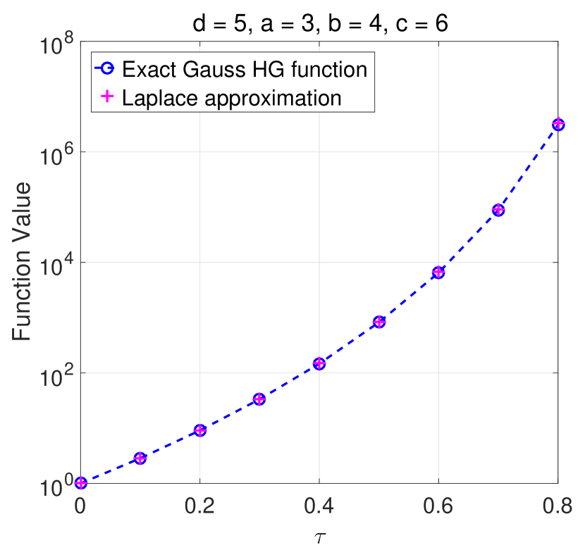
(a)

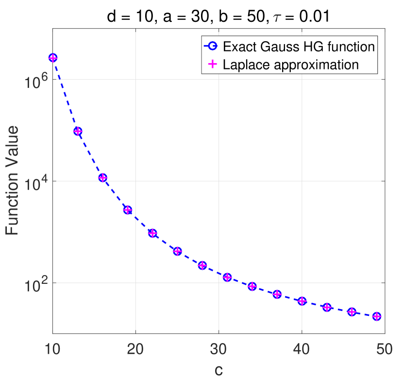
(b)

Figure 8: Exact values of function $\leavevmode\nobreak\ {}_{2}F_{1}(a,b;c;\tau I_{d})$ and its corresponding Laplace approximation $\leavevmode\nobreak\ {}_{2}\hat{F}_{1}(a,b;c;\tau I_{d})$ versus: (a) $\tau$, for $d=5$, $a=3$, $b=4$, and $c=6$, (b) $c$, for $d=10$, $a=30$, $b=50$, and $\tau=0.01$.

References

- [1] S. J. Pan and Q. Yang, “A survey on transfer learning,” IEEE Transactions on knowledge and data engineering, vol. 22, no. 10, pp. 1345–1359, 2010.
- [2] H. Venkateswara, S. Chakraborty, and S. Panchanathan, “Deep-learning systems for domain adaptation in computer vision: Learning transferable feature representations,” IEEE Signal Processing Magazine, vol. 34, no. 6, pp. 117–129, 2017.
- [3] V. M. Patel, R. Gopalan, R. Li, and R. Chellappa, “Visual domain adaptation: A survey of recent advances,” IEEE signal processing magazine, vol. 32, no. 3, pp. 53–69, 2015.
- [4] K. Weiss, T. M. Khoshgoftaar, and D. Wang, “A survey of transfer learning,” Journal of Big Data, vol. 3, no. 1, p. 9, 2016.
- [5] G. Csurka, “Domain adaptation for visual applications: A comprehensive survey,” arXiv preprint arXiv:1702.05374, 2017.
- [6] N. Zou, Y. Zhu, J. Zhu, M. Baydogan, W. Wang, and J. Li, “A transfer learning approach for predictive modeling of degenerate biological systems,” Technometrics, vol. 57, no. 3, pp. 362–373, 2015.
- [7] P. Ganchev, D. Malehorn, W. L. Bigbee, and V. Gopalakrishnan, “Transfer learning of classification rules for biomarker discovery and verification from molecular profiling studies,” Journal of biomedical informatics, vol. 44, pp. S17–S23, 2011.
- [8] B. Gong, Y. Shi, F. Sha, and K. Grauman, “Geodesic flow kernel for unsupervised domain adaptation,” in Computer Vision and Pattern Recognition (CVPR), 2012 IEEE Conference on. IEEE, 2012, pp. 2066–2073.
- [9] L. Duan, D. Xu, and I. Tsang, “Learning with augmented features for heterogeneous domain adaptation,” ICML, 2012.
- [10] J. Hoffman, E. Rodner, T. Darrell, J. Donahue, and K. Saenko, “Efficient learning of domain-invariant image representations,” in International Conference on Learning Representations (ICLR), 2013.
- [11] J. Hoffman, E. Rodner, J. Donahue, B. Kulis, and K. Saenko, “Asymmetric and category invariant feature transformations for domain adaptation,” International journal of computer vision, vol. 109, no. 1-2, pp. 28–41, 2014.
- [12] Y.-H. Hubert Tsai, Y.-R. Yeh, and Y.-C. Frank Wang, “Learning cross-domain landmarks for heterogeneous domain adaptation,” in Proceedings of the IEEE Conference on Computer Vision and Pattern Recognition, 2016, pp. 5081–5090.
- [13] K. M. Borgwardt, A. Gretton, M. J. Rasch, H.-P. Kriegel, B. Schölkopf, and A. J. Smola, “Integrating structured biological data by kernel maximum mean discrepancy,” Bioinformatics, vol. 22, no. 14, pp. e49–e57, 2006.
- [14] W. Dai, Q. Yang, G.-R. Xue, and Y. Yu, “Boosting for transfer learning,” in Proceedings of the 24th international conference on Machine learning. ACM, 2007, pp. 193–200.
- [15] L. Duan, I. W. Tsang, D. Xu, and S. J. Maybank, “Domain transfer svm for video concept detection,” in Computer Vision and Pattern Recognition, 2009. CVPR 2009. IEEE Conference on. IEEE, 2009, pp. 1375–1381.
- [16] L. Bruzzone and M. Marconcini, “Domain adaptation problems: A dasvm classification technique and a circular validation strategy,” IEEE transactions on pattern analysis and machine intelligence, vol. 32, no. 5, pp. 770–787, 2010.
- [17] S. Herath, M. Harandi, and F. Porikli, “Learning an invariant hilbert space for domain adaptation,” in 2017 IEEE Conference on Computer Vision and Pattern Recognition (CVPR), July 2017, pp. 3956–3965.
- [18] N. Courty, R. Flamary, D. Tuia, and A. Rakotomamonjy, “Optimal transport for domain adaptation,” IEEE Transactions on Pattern Analysis and Machine Intelligence, vol. 39, no. 9, pp. 1853–1865, Sept 2017.
- [19] M. Long, Y. Cao, J. Wang, and M. Jordan, “Learning transferable features with deep adaptation networks,” in International Conference on Machine Learning, 2015, pp. 97–105.
- [20] M. Long, H. Zhu, J. Wang, and M. I. Jordan, “Unsupervised domain adaptation with residual transfer networks,” in Advances in Neural Information Processing Systems, 2016, pp. 136–144.
- [21] Y. Ganin, E. Ustinova, H. Ajakan, P. Germain, H. Larochelle, F. Laviolette, M. Marchand, and V. Lempitsky, “Domain-adversarial training of neural networks,” Journal of Machine Learning Research, vol. 17, no. 59, pp. 1–35, 2016.
- [22] M.-Y. Liu and O. Tuzel, “Coupled generative adversarial networks,” in Advances in neural information processing systems, 2016, pp. 469–477.
- [23] L. A. Dalton and E. R. Dougherty, “Optimal classifiers with minimum expected error within a Bayesian framework—Part I: Discrete and gaussian models,” Pattern Recognition, vol. 46, no. 5, pp. 1288 – 1300, 2013.
- [24] ——, “Optimal classifiers with minimum expected error within a Bayesian framework — Part II: Properties and performance analysis,” Pattern Recognition, vol. 46, no. 5, pp. 1301 – 1314, 2013.
- [25] R. J. Muirhead, Aspects of multivariate statistical theory. John Wiley & Sons, 2009.
- [26] K. Halvorsen, V. Ayala, and E. Fierro, “On the marginal distribution of the diagonal blocks in a blocked Wishart random matrix,” International Journal of Analysis, vol. 2016, pp. 1–5, 2016.
- [27] D. K. Nagar and J. C. Mosquera-Benıtez, “Properties of matrix variate hypergeometric function distribution,” Applied Mathematical Sciences, vol. 11, no. 14, pp. 677–692, 2017.
- [28] A. G. Constantine, “Some non-central distribution problems in multivariate analysis,” Ann. Math. Statist., vol. 34, no. 4, pp. 1270–1285, 12 1963.
- [29] R. W. Butler and A. T. A. Wood, “Laplace approximations for hypergeometric functions with matrix argument,” The Annals of Statistics, vol. 30, no. 4, pp. 1155–1177, 2002.
- [30] L. A. Dalton and M. R. Yousefi, “On optimal Bayesian classification and risk estimation under multiple classes,” EURASIP Journal on Bioinformatics and Systems Biology, vol. 2015, no. 1, p. 8, 2015.
- [31] L. A. Dalton and E. R. Dougherty, “Bayesian minimum mean-square error estimation for classification error-Part I: Definition and the Bayesian MMSE error estimator for discrete classification,” IEEE Transactions on Signal Processing, vol. 59, no. 1, pp. 115–129, Jan 2011.
- [32] K. Saenko, B. Kulis, M. Fritz, and T. Darrell, “Adapting visual category models to new domains,” in Proceedings of the 11th European Conference on Computer Vision: Part IV, ser. ECCV’10. Berlin, Heidelberg: Springer-Verlag, 2010, pp. 213–226.
- [33] G. Griffin, A. Holub, and P. Perona, “Caltech-256 object category dataset,” Technical Report 7694, California Institute of Technology, 2007.
- [34] H. Bay, T. Tuytelaars, and L. Van Gool, “SURF: Speeded up robust features,” Computer vision–ECCV 2006, pp. 404–417, 2006.
- [35] J. M. Knight, I. Ivanov, and E. R. Dougherty, “MCMC implementation of the optimal Bayesian classifier for non-Gaussian models: Model-based RNA-seq classification,” BMC bioinformatics, vol. 15, no. 1, p. 401, 2014.
- [36] J. M. Knight, I. Ivanov, K. Triff, R. S. Chapkin, and E. R. Dougherty, “Detecting multivariate gene interactions in RNA-seq data using optimal Bayesian classification,” IEEE/ACM transactions on computational biology and bioinformatics, 2015.
- [37] A. Karbalayghareh, U. Braga-Neto, J. Hua, and E. R. Dougherty, “Classification of state trajectories in gene regulatory networks,” IEEE/ACM Transactions on Computational Biology and Bioinformatics, vol. 15, no. 1, pp. 68–82, Jan 2018.
- [38] A. Karbalayghareh, U. Braga-Neto, and E. R. Dougherty, “Classification of single-cell gene expression trajectories from incomplete and noisy data,” IEEE/ACM Transactions on Computational Biology and Bioinformatics, vol. PP, no. 99, pp. 1–1, 2018.
- [39] ——, “Classification of gaussian trajectories with missing data in boolean gene regulatory networks,” in 2017 IEEE International Conference on Acoustics, Speech and Signal Processing (ICASSP), March 2017, pp. 1078–1082.
- [40] ——, “Intrinsically bayesian robust classifier for single-cell gene expression trajectories in gene regulatory networks,” BMC Systems Biology, vol. 12, no. 3, p. 23, Mar 2018.
- [41] L. A. Dalton and E. R. Dougherty, “Application of the Bayesian MMSE estimator for classification error to gene expression microarray data,” Bioinformatics, vol. 27, no. 13, pp. 1822–1831, 2011.
- [42] M. S. Esfahani and E. R. Dougherty, “Incorporation of biological pathway knowledge in the construction of priors for optimal Bayesian classification,” IEEE/ACM Transactions on Computational Biology and Bioinformatics, vol. 11, no. 1, pp. 202–218, Jan 2014.
- [43] ——, “An optimization-based framework for the transformation of incomplete biological knowledge into a probabilistic structure and its application to the utilization of gene/protein signaling pathways in discrete phenotype classification,” IEEE/ACM Transactions on Computational Biology and Bioinformatics, vol. 12, no. 6, pp. 1304–1321, Nov 2015.
- [44] S. Boluki, M. S. Esfahani, X. Qian, and E. R. Dougherty, “Incorporating biological prior knowledge for bayesian learning via maximal knowledge-driven information priors,” BMC Bioinformatics, vol. 18, no. 14, p. 552, Dec 2017.
- [45] L. A. Dalton and E. R. Dougherty, “Intrinsically optimal Bayesian robust filtering,” IEEE Transactions on Signal Processing, vol. 62, no. 3, pp. 657–670, Feb 2014.
- [46] X. Qian and E. R. Dougherty, “Bayesian regression with network prior: Optimal Bayesian filtering perspective,” IEEE Transactions on Signal Processing, vol. 64, no. 23, pp. 6243–6253, Dec 2016.
- [47] R. Dehghannasiri, M. S. Esfahani, and E. R. Dougherty, “Intrinsically Bayesian robust Kalman filter: An innovation process approach,” IEEE Transactions on Signal Processing, vol. 65, no. 10, pp. 2531–2546, May 2017.
- [48] D. K. Nagar and S. Nadarajah, “Appell’s hypergeometric functions of matrix arguments,” Integral Transforms and Special Functions, vol. 28, no. 2, pp. 91–112, 2017.
- [49] A. K. Gupta, D. K. Nagar, and L. E. Sánchez, “Properties of matrix variate confluent hypergeometric function distribution,” Journal of Probability and Statistics, vol. 2016, 2016.