Direct Measurement of Astrophysically Important Resonances in ${}^{38}\mathrm{K}(p,\gamma){}^{39}\mathrm{Ca}$

Abstract

Background

Classical novae are cataclysmic nuclear explosions occurring when a white dwarf in a binary system accretes hydrogen-rich material from its companion star. Novae are partially responsible for the galactic synthesis of a variety of nuclides up to the calcium ($A\sim 40$) region of the nuclear chart. Although the structure and dynamics of novae are thought to be relatively well understood, the predicted abundances of elements near the nucleosynthesis endpoint, in particular Ar and Ca, appear to sometimes be in disagreement with astronomical observations of the spectra of nova ejecta.

Purpose

One possible source of the discrepancies between model predictions and astronomical observations is nuclear reaction data. Most reaction rates near the nova endpoint are estimated only from statistical model calculations, which carry large uncertainties. For certain key reactions, these rate uncertainties translate into large uncertainties in nucleosynthesis predictions. In particular, the ${}^{38}\mathrm{K}\left(p,\gamma\right){}^{39}\mathrm{Ca}$ reaction has been identified as having a significant influence on Ar, K, and Ca production. In order to constrain the rate of this reaction, we have performed a direct measurement of the strengths of three candidate $\ell=0$ resonances within the Gamow window for nova burning, at $386\pm 10$ keV, $515\pm 10$ keV, and $689\pm 10$ keV.

Method

The experiment was performed in inverse kinematics using a beam of unstable ${}^{38}\mathrm{K}$ impinged on a windowless hydrogen gas target. The ${}^{39}\mathrm{Ca}$ recoils and prompt $\gamma$ rays from ${}^{38}\mathrm{K}\left(p,\gamma\right){}^{39}\mathrm{Ca}$ reactions were detected in coincidence using a recoil mass separator and a bismuth-germanate scintillator array, respectively.

Results

For the $689$ keV resonance, we observed a clear recoil-$\gamma$ coincidence signal and extracted resonance strength and energy values of $120^{+50}_{-30}~{}\mathrm{(stat.)}^{+20}_{-60}~{}\mathrm{(sys.)}~{}\mathrm{meV}$ and $679^{+2}_{-1}~{}\mathrm{(stat.)}\pm 1~{}\mathrm{(sys.)}~{}\mathrm{keV}$, respectively. We also performed a singles analysis of the recoil data alone, extracting a resonance strength of $120\pm 20~{}\mathrm{(stat.)}\pm 15~{}\mathrm{(sys.)}$ meV, consistent with the coincidence result. For the $386$ keV and $515$ keV resonances, we extract $90\%$ confidence level upper limits of $2.54$ meV and $18.4$ meV, respectively.

Conclusions

We have established a new recommended ${}^{38}\mathrm{K}(p,\gamma){}^{39}\mathrm{Ca}$ rate based on experimental information, which reduces overall uncertainties near the peak temperatures of nova burning by a factor of $\sim 250$. Using the rate obtained in this work in model calculations of the hottest oxygen-neon novae reduces overall uncertainties on Ar, K, and Ca synthesis to factors of $15$ or less in all cases.

I Introduction

Classical novae are some of the most common explosive stellar events to occur in our galaxy, with an estimated frequency of $35\pm 11$ per year Shafter (1997). Novae happen when a white dwarf in a binary system accretes hydrogen-rich material from its main-sequence companion, igniting thermonuclear runaway. Observations of the spectra of ejected material indicate that two main classes of nova exist, depending on the initial composition of the underlying white dwarf: carbon-oxygen (CO) and oxygen-neon (ONe). Model calculations indicate that ONe novae, which occur on more massive white dwarves, can reach peak temperatures around $0.4$ GK and synthesize nuclei up to the calcium region ($A\sim 40$). At present, there are a number of outstanding discrepancies between astronomical observations of the spectra of nova ejecta Pottasch (1959); Andrea et al. (1994); Arkhipova et al. (2000); Evans et al. (2003) and nova model predictions José et al. (2006); Starrfield et al. (2009). In particular, the model predictions of Ref. Starrfield et al. (2009) indicate Ar and Ca abundances at roughly the solar level, while in contrast the observations of Ref. Andrea et al. (1994) point towards nova ejecta with Ar and Ca abundances around an order of magnitude greater than solar. Resolution of such discrepancies requires that nova models be capable of making detailed predictions regarding the synthesis of nuclides in the Ar–Ca region. In turn, this requires improved constraints on the rates of key nuclear reactions involved in nova nucleosynthesisis, in particular for reactions near the nucleosynthesis endpoint.

In 2002, Iliadis et al. published a seminal paper investigating the influence of nuclear reaction rate variations on nucleosynthesis in classical novae Iliadis et al. (2002). In this study, the authors varied the rates of $64$ nuclear reactions within their recommended uncertainties and examined the effect of these variations on the nucleosynthesis predictions of seven different nova models. For the hottest model included in the study, reaching a peak temperature of $0.418$ GK, the authors identified the ³⁸K$(p,\gamma)^{39}$Ca reaction as having a significant influence on the production of Ar, K, and Ca. Qualitatively, the predicted abundances of these elements were found to vary by respective factors of $24$, $58$, and $57$ when the ³⁸K$(p,\gamma)^{39}$Ca rate was varied within its existing uncertainties. When Ref. Iliadis et al. (2002) was published, the ³⁸K$(p,\gamma)^{39}$Ca rate was estimated entirely from statistical model predictions with no experimental nuclear physics input Iliadis et al. (2001). This rate estimate was assigned an overall uncertainty of $10^{4}$, i.e. the upper and lower limits were established at $100$ and $0.01$ times the central value, respectively. The importance of this reaction for nova nucleosynthesis, along with the paucity of experimental input regarding the accepted rate, prompted an attempt by the present authors to measure the strengths of the three $\ell=0$ resonances lying within the Gamow window for ONe novae ($T_{\mathrm{peak}}\simeq 0.2$–$0.4$ GK). The first results of this study were published in a review article Brune and Davids (2015) and a recent Letter, which recommends a new, experimentally-based rate with uncertainties over two orders of magnitude smaller than before Lotay et al. (2016). In the present Article, we expand upon Ref. Lotay et al. (2016), providing significantly more detail concerning the experiment and data analysis. We also report the results of a new sensitivity study investigating the effect of our measurement on the synthesis of Ar, K, and Ca in classical novae. The results presented here supersede those published previously.

II Experiment

The experiment was performed in the ISAC-I Laxdal (2003) hall at Triumf, Canada’s national laboratory for particle and nuclear physics. A beam of radioactive ³⁸K was produced by impinging $500$ MeV protons from the Triumf cyclotron onto a high-power TiC production target. The ³⁸K⁽¹⁺⁾ ions produced by spallation reactions in the target were extracted and sent through a high-resolution mass separator. They were then charge bred to the $7^{+}$ charge state in an electron cyclotron resonance (ECR) charge state booster before post-acceleration. The charge breeding is necessary because the ISAC-I radio frequency quadrupole (RFQ) is restricted to a mass-to-charge ratio of $30$ or less Ames et al. (2014).

The ³⁸K⁽⁷⁺⁾ beam was delivered to the Detector of Recoils and Gammas of Nuclear Reactions (DRAGON) where it impinged on a windowless extended gas target Hutcheon et al. (2003), filled with H₂ at an average pressure and temperature of $10.6$ mbar and $298$ Kelvin, respectively. The H₂ was cleaned by continuous recirculation through a LN₂ cooled zeolite trap. The prompt $\gamma$ rays from ³⁸K$(p,\gamma)^{39}$Ca reactions were detected in array of $30$ bismuth germanate (BGO) scintillators surrounding the target, while the ³⁹Ca recoils were transmitted to the focal plane of DRAGON, separating them from unreacted and elastically scattered ³⁸K. A timing signature for recoils was established as the time difference between signals from a pair of microchannel plates separated by $59$ cm, which detected secondary electrons produced by the interaction of the recoil ions with a diamond-like carbon foil intersecting the beam line. The total kinetic energy and stopping power of the recoil ions was measured in a multi-anode ionization chamber (IC) Vockenhuber et al. (2009). Coincidences between recoils and prompt $\gamma$ rays were identified using a timestamp-based algorithm Christian et al. (2014). The ³⁹Ca recoils were separated from a background of scattered and charge-changed ³⁸K (“leaky beam”) based primarily on the local time of flight (TOF) between the two MCPs (“MCP TOF”) and the time difference between the $\gamma$ ray and the upstream MCP (“separator TOF”).

Laboratory beam energies of $15.58$ MeV, $20.56$ MeV, and $27.17$ MeV were employed for measurements of the $386\pm 10$ keV, $515\pm 10$ keV, and $689\pm 10$ keV resonances, respectively. The beam energies were measured using the procedure given in Ref. Hutcheon et al. (2012). The beam was centered on $2$ mm slits downstream of DRAGON’s first magnetic dipole, and the measured field value was converted to energy by solving the relativistically-correct equation,

$$E/A=c_{\mathrm{mag}}\left(qB/A\right)^{2}-\frac{1}{2uc^{2}}\left(E/A\right)^{2},$$ (1)

where $E$, $A$, and $q$ are the beam kinetic energy, mass number, and charge state, respectively, and $u$ is the atomic mass unit. The quantity $c_{\mathrm{mag}}$ is related to the effective bending radius of the dipole. The recommended value from Ref. Hutcheon et al. (2012), $c_{\mathrm{mag}}=48.15\pm 0.07$ MeV$\cdot$T², was employed for this experiment. The estimated uncertainty on this procedure is $0.17\%.$

The chosen beam energies cover respective center-of-mass energies in the DRAGON gas target of $386\pm 13$, $515\pm 13$, and $689\pm 13$ keV. The resonances in question were previously identified as $5/2^{+}$ ³⁹Ca states through ⁴⁰Ca$({}^{3}\mathrm{He},\alpha)^{39}$Ca Hinds and Middleton (1966), ⁴⁰Ca$(d,t)^{39}$Ca Doll et al. (1976), and ⁴⁰Ca$(p,d)^{39}$Ca Matoba et al. (1993) transfer reaction studies. Their recommended excitation energies are $6157\pm 10$, $6286\pm 10$, and $6460\pm 10$ keV, corresponding to ³⁸K$+p$ resonances at $386\pm 10$, $515\pm 10$, and $689\pm 10$ keV, respectively Singh and Cameron (2006). The respective $(p,\gamma)$ cone angles for measurements at the $15.58$ MeV, $20.56$ MeV, and $27.17$ MeV beam energies were $5.98$ mrad, $5.29$ mrad, and $4.73$ mrad. Each of these is well within the $\pm 21$ mrad angular acceptance of DRAGON Ruiz et al. (2014).

For each beam energy, only a single charge state was transmitted to the end of DRAGON. The respective charge states were $7^{+}$, $9^{+}$, and $10^{+}$ for the $15.58$ MeV, $20.56$ MeV, and $27.17$ MeV beam energies. The charge state fractions and stopping powers for K and Ca ions passing through the gas target were measured separately using stable beams of ³⁹K and ⁴⁴Ca. Charge state fractions were determined by measuring the ratio $({I_{2}^{{g}}}/{I_{0}^{{g}}})\cdot({I_{0}^{{ng}}}/{I_{1}^{{ng}}}),$ where $I_{0}$, $I_{1}$, and $I_{2}$ represent the current on Faraday cups upstream of the gas target, downstream of the gas target, and downstream of the first magnetic dipole, respectively; and the superscripts $g$ and $ng$ represent currents measured with and without gas in the target, respectively. Current measurements were taken with the magnetic dipole set to accept each of the charge states that resulted in a measurable $I_{2}$. The resulting distributions were then fit with a Gaussian function (normalized to unity). The value of the Gaussian at each charge state was taken to represent the corresponding charge state fraction. Measurements were taken at three different beam energies spanning the range of beam energies employed in the experiment, and the resulting charge fractions were fit with a quadratic function. The value of this quadratic function at the various beam energies employed in the experiment was then taken as the charge state fraction to use in the recoil yield analysis. All fits were performed using MINUIT and errors on the fit parameters were calculated using MINOS James and Roos (1975). The errors on the Gaussian fit were propagated along with the errors on the quadratic interpolation to arrive at the final error on the charge state fractions used in the analysis.

The number of incoming ³⁸K⁽⁷⁺⁾ ions was determined by counting delayed ($t_{1/2}=$ $7.6$ minutes) $2.2$ MeV $\gamma$ rays emitted by the daughters of beam ions implanted into the mass slits just downstream of DRAGON’s first electric dipole. These $\gamma$ rays were detected in a NaI scintillator with an efficiency of $(8.46\pm 0.95)\times 10^{-6}$. This efficiency was determined from a Geant4 Agostinelli et al. (2003) simulation, which included the entire geometry of the mass slit box and NaI detector. The $11\%$ relative uncertainty on the NaI efficiency was determined by comparing simulation results to known ²²Na and ¹³⁷Cs source measurements. This analysis includes an uncertainty on the source position of $\pm 0.5$ cm. The average beam rate for each ${\sim}1$ hour run was determined by fitting the decay rate vs. time curves with the expected response function,

$$A(t)=I\left(1-e^{-\lambda t}\right)+N_{0}\lambda e^{-\lambda t},$$ (2)

where $A(t)$ is the decay rate, $I$ is the average beam intensity, $N_{0}$ is the initial number of particles implanted in the slit, and $\lambda=1.5\times 10^{-3}$ s^-1 is the ³⁸K decay constant. In the fit, both $I$ and $N_{0}$ were allowed to vary as free parameters. Cases where the average beam rate fluctuated significantly over the course of a run were identified by a noticeable deviation from the expected response. These fluctuations in the beam rate (or the complete loss of beam delivery) arose from a number of sources upstream of the DRAGON target, for example loss of the $500$ MeV proton beam or Faraday cup readings taken by the ISAC-I operators. In these cases, differing sections of the run were visually identified and independently fit to Eq. (2). Figure 1(a) shows sample fitted rate vs. time curves for two runs, one with a constant beam rate and the other with a varying beam rate (and corresponding piecewise fit). Figure 1(b) shows the average beam rates determined for each run throughout the course of the experiment. The overall ³⁸K rate was approximately $2\times 10^{7}$ particles per second.

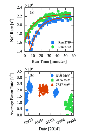
Figure 1: (a) Sample rate vs. time curves measured in the NaI detector. The green filled circles correspond to a run where the beam rate was constant, while the blue filled squares correspond to a run where there were significant changes in the rate. The solid orange lines show the fit results used to extract the average beam intensities. (b) Average beam rate determined for each ${\sim}1$ hour run taken during the experiment. The filled circles, rectangles, and triangles denote each run’s beam energy, as indicated in the legend.

II.1 386(10) keV and 515(10) keV Resonances

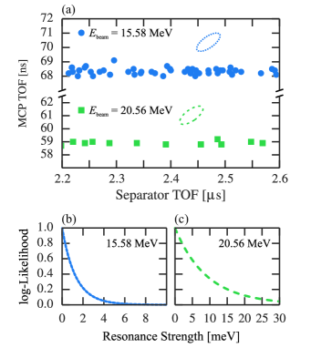
Figure 2: (a) MCP vs. separator TOF for the $15.58$ MeV and $20.56$ MeV beam energies. The blue dotted and green dashed ovals represent the expected location of recoils for the $15.58$ MeV and $20.56$ MeV beam energies, respectively. (b) Profile likelihood curve for the $15.58$ MeV beam energy. (c) Profile likelihood curve for the $20.56$ MeV beam energy.

At beam energies of $15.58$ MeV and $20.56$ MeV (corresponding to the $386\pm 10$ keV and $515\pm 10$ keV resonances, respectively), we observed zero events in the expected recoil region. This is demonstrated in Figure 2(a), which shows MCP vs. separator TOF spectra for each of the $15.58$ MeV and $20.56$ MeV beam energies. The dashed and dotted ellipses included on the plots indicate the expected location of ³⁹Ca recoils, based on Geant3 simulations of the reaction and transmission through the DRAGON separator. As can be seen, in both cases no recoil events fall within this expected window. As a result, we extracted upper limits on the resonance strengths using a modification of the Rolke profile likelihood method for calculating confidence intervals in the presence of uncertain background rates and detection efficiencies Rolke et al. (2005). In the standard Rolke treatment, the likelihood is the product of the individual likelihoods describing the signal rate $\mu$, background rate $b$ (both treated as Poisson), and the detection efficiency $\eta$ (treated as Gaussian with uncertainty $\sigma_{\eta}$). Mathematically, this is expressed as

$$\mathscr{L}(\mu,b,\eta|x,y,z)=\\ \left[{\frac{\left({\eta\mu+b}\right)^{x}}{x!}e^{\eta\mu+b}}\right]\left[{\frac{\left({b\tau}\right)^{y}}{y!}e^{b\tau}}\right]\left[{\frac{e^{\left({z-\eta}\right)^{2}/\left({2\sigma_{\eta}}\right)}}{\sqrt{2\pi}\sigma_{\eta}}}\right],$$ (3)

where $x$ is the number of events observed in the signal region, $y$ is the number of events observed in a background region that is $\tau$ times as large as the signal region, and $z$ is the observed signal rate. Equation (3) is then maximized with respect to $b$ and $\eta$ to construct a one-dimensional likelihood curve that is a function of only the signal strength $\mu$ and can be analyzed to extract upper limits.

In the present analysis, we extend the Rolke method to also account for uncertainties in the resonance energy $E_{r}$, the number of incoming beam particles $N$, and the ³⁸K + H₂ stopping power $\epsilon$. Each of these quantities factors into the calculation of the resonance strength, and hence their uncertainties should be included for a complete treatment of the problem. For each of these quantities, we treat the uncertainty as Gaussian (with widths $\sigma_{E}$, $\sigma_{N}$, and $\sigma_{\epsilon}$, respectively). The complete likelihood function is then given by

$$\mathscr{L}\left({\omega\gamma,b,\eta,E_{r},N,\epsilon|x,y,z,E_{r0},N_{0},\epsilon_{0}}\right)=\\ \left[{\frac{\left({\eta\mu+b}\right)^{x}}{x!}e^{\eta\mu+b}}\right]\left[{\frac{\left({b\tau}\right)^{y}}{y!}e^{b\tau}}\right]\left[{\frac{e^{\left({z-\eta}\right)^{2}/\left({2\sigma_{\eta}}\right)}}{\sqrt{2\pi}\sigma_{\eta}}}\right]\times\\ \left[{\frac{e^{\left({E_{r_{0}}-E_{r}}\right)^{2}/\left({2\sigma_{E}}\right)}}{\sqrt{2\pi}\sigma_{E}}}\right]\left[{\frac{e^{\left({N_{0}-N}\right)^{2}/\left({2\sigma_{N}}\right)}}{\sqrt{2\pi}\sigma_{N}}}\right]\left[{\frac{e^{\left({\epsilon_{0}-\epsilon}\right)^{2}/\left({2\sigma_{\epsilon}}\right)}}{\sqrt{2\pi}\sigma_{\epsilon}}}\right],$$ (4)

where $E_{r_{0}}$, $N_{0}$, and $\epsilon_{0}$ are the observed central values of the resonance energy, beam ions on target, and stopping power, respectively. In Eq. (4), the signal rate $\mu$ is no longer a constant parameter but rather a function of the resonance strength $\omega\gamma$, resonance energy $E_{r}$, number of incoming beam particles $N$, center-of-mass stopping power $\epsilon$, beam mass $M$, and target mass $m$,

$$\mu(\omega\gamma,E_{r},N,\epsilon)=\frac{N\left({\omega\gamma}\right)\left({hc}\right)^{2}}{2\epsilon\left[{E_{r}^{2}+2E_{r}mM/\left({m+M}\right)}\right]}.$$ (5)

Following the Rolke prescription, we maximize Eq. (4) with respect to the “nuisance” parameters $\left\{{b,\eta,E_{r},N,\epsilon}\right\}$ to arrive at a profile likelihood that is a function of only the resonance strength $\omega\gamma$. In practice, we first take the negative logarithm of Eq. (4) and then calculate the minimum numerically using the MINUIT package James and Roos (1975). The resulting profile likelihoods for the $15.58$ MeV and $20.56$ MeV beam energies are shown in Figures 2(b) and 2(c), respectively (plotted as negative log-likelihoods). To extract single-sided $68\%$, $90\%$, and $95\%$ upper limits from the profile likelihood curves, we follow exactly the prescriptions of Ref. Rolke et al. (2005). The resulting upper limits, along with all of the measured parameters going into the upper limit calculation are summarized in Tables 1 and 2. It should be noted that when we refer to “$68\%$” or “$95\%$” confidence intervals, we mean the area under a normalized gaussian distribution between the $\pm 1\sigma$ or $\pm 2\sigma$ limits. These are more precisely equal to $68.27\%$ and $95.45\%$, respectively.

Table 1: Summary of observed quantities going into the resonance strength upper limit calculations, for the $15.58$ MeV beam energy.

Quantity	Value
Background rate	$4.44\times 10^{-2}$
Beam ions on target	$(2.88\pm 0.36)\times 10^{12}$
Stopping power [eV cm2]	$(3.78\pm 0.14)\times 10^{-15}$
Detection efficiency	$0.093\pm 0.016$
$68\%$ upper limit [meV]	$1.16$
$90\%$ upper limit [meV]	$2.54$
$95\%$ upper limit [meV]	$3.53$

Table 2: Summary of observed quantities going into the resonance strength upper limit calculations, for the $20.56$ MeV beam energy.

Quantity	Value
Background rate	$4.44\times 10^{-3}$
Beam ions on target	$(8.8\pm 1.2)\times 10^{11}$
Stopping power [eV cm2]	$(4.04\pm 0.14)\times 10^{-15}$
Detection efficiency	$0.062\pm 0.011$
$68\%$ upper limit [meV]	$8.59$
$90\%$ upper limit [meV]	$18.4$
$95\%$ upper limit [meV]	$25.5$

II.2 689(10) keV Resonance

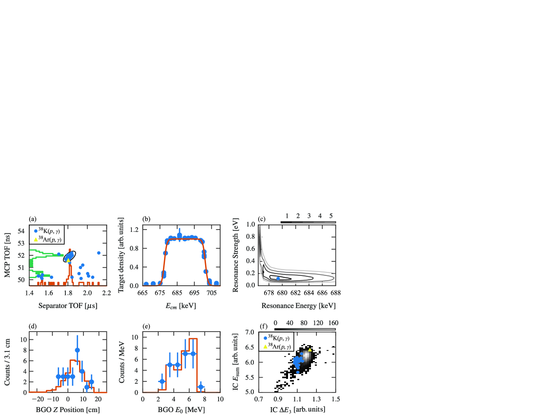
Figure 3: Summary of the coincidence analysis for the data taken with a beam energy of $27.17$ MeV. The individual descriptions of panels (a) through (f) are as follows: a) Separator vs. MCP TOF particle identification spectrum. The blue filled circles represent data collected with the radioactive ³⁸K beam, while the single filled yellow triangle represents data collected with a ³⁸Ar beam, for background characterization. The open ellipse outlines the expected recoil region. Projections onto the horizontal and vertical axes are also included (as the unshaded orange and green histograms). b) Target density as a function of center-of-mass beam energy. The filled circles with error bars represent the data points and the solid line shows the fit to Eq. (7). c) NLL contour plot, calculated by comparing simulated and measured BGO $z$ positions as explained in the text. The solid blue point shows the location of the global minimum. d) Measured BGO $z$-position distribution for recoil events (filled circles), compared with the best-fit simulation result at $E_{r}=679$ keV and $\omega\gamma=120$ eV (solid orange lines). e) Same as panel (d), but showing the measured energy of the most energetic $\gamma$-ray hit in the BGO array. f) Total energy deposited in the IC vs. energy loss in the third (most downstream) anode. The filled (blue) circles show the location of the ³⁹Ca coincidence recoils observed with the ³⁸K beam. The filled yellow triangle denotes the location of the event observed with a beam of pure ³⁸Ar. The greyscale color map shows the location of all heavy-ion singles events observed with the $27.17$ MeV ³⁸K beam. This distribution is dominated by leaky beam.

In contrast to the two lower-energy resonances, we observed a clear recoil signal when running with a beam energy of $27.17$ MeV. This is demonstrated in the separator TOF vs. MCP TOF distribution shown by the filled circles in Figure 3(a). This spectrum exhibits a clear clustering of $27$ recoil events in the region indicated by the open ellipse. The BGO $z$-position distribution of the identified recoil events is clustered downstream of the target center, indicating a resonance energy less than the central value of $689$ keV Hutcheon et al. (2012). Hence to extract a resonance strength, $\omega\gamma,$ and a resonance energy, $E_{r}$, we use a technique similar to that employed in Ref. Erikson et al. (2010). For a fixed beam energy of $27.17$ MeV, we generate a simulated BGO $z$-position spectrum over the range of resonance energies contained within the gas target. For the simulations, we use the standard DRAGON Geant3 package Gigliotti (2004) and convolute the resulting BGO energies with a realistic hardware threshold. The hardware threshold was determined experimentally by taking long background runs with the threshold set to the value employed in the experiment, and to a reduced value of $50$ mV. The resulting spectra were normalized, divided into each other, and fit with a Fermi function to arrive at the functional form used in the analysis. Following the threshold convolution, we scale the simulated spectra by the factor

$$\eta Y_{\omega\gamma}\left.{N_{b}}\middle/{N_{\mathrm{sim}}}\right.,$$ (6)

where $\eta=0.121\pm 0.003$ is the heavy-ion detection efficiency, $Y_{\omega\gamma}$ is the reaction yield at a given resonance strength $\omega\gamma$, $N_{b}=(2.53\pm 0.30)\times 10^{12}$ is the number of incoming beam ions, and $N_{\mathrm{sim}}=50,000$ is the number of simulated events. Scaled in this manner, the simulated spectrum represents both the magnitude and the shape of the BGO $z$-position distribution for a given $\omega\gamma$ and $E_{r}$.

The $\gamma$-ray efficiency is implicitly included in the generation of the simulated spectra since the number of counts appearing in the spectra prior to scaling is determined by the detection efficiency, as modeled in the Geant3 simulation. This modeling is sensitive to the branching ratios for $\gamma$-ray decay from the $6460$ keV state in ³⁹Ca. These branching ratios have not been measured, and hence we have assumed dominant decays either directly to the ground state or through the first excited $\nicefrac{{5}}{{2}}^{-}$ state, as observed for the decay of known $\nicefrac{{5}}{{2}}^{+}$ excited states in the well-studied mirror nucleus ³⁹K Singh and Cameron (2006). The location of the $\nicefrac{{5}}{{2}}_{1}^{-}$ state in ³⁹Ca has not been conclusively assigned, but there are a number of candidates in the ${\sim}3$–$4$ MeV excitation energy region Singh and Cameron (2006). Hence for the present analysis, we have assumed decay through a state at $3.5$ MeV to represent the feeding through the $\nicefrac{{5}}{{2}}_{1}^{-}$. To quantatively account for the uncertainty related to the $\gamma$-ray decay scheme, we have utilized a profile likelihood technique to marginalize over the unknown branching ratios. Specifically, we performed separate simulations for a range of different fractional feedings directly to the ground state or through a state at $3.5$ MeV. In the simulations, the ground state/excited state ratios ranged from $0\%$–$100\%$ in steps of $10\%$. For each set of simulations, we took the branching with the highest likelihood value and incorporated it into the eventual likelihood surface used to extract confidence intervals on the resonance strength and energy (the calculation of likelihoods and construction of the likelihood surface is detailed later in this section). This technique of using profile likelihoods to marginalize over relevant, but uninteresting “nuisance” parameters is well established in the statistical literature; see, for example Refs. Rolke et al. (2005); James (2006). It should be noted that the uncertainty on the $\gamma$-ray detection efficiency is dominated by geometrical and Monte-Carlo uncertainties and not the unknown branching ratios.

The yield parameter in Eq. (6), $Y_{\omega\gamma}$, is given by the convolution of the standard Breit-Wigner narrow-resonance cross section Iliadis (2007) with the gas target density profile. The density profile was measured in a previous experiment by recording the $\gamma$-ray yield from the ${}^{3}\mathrm{He}({}^{12}\mathrm{C},p){}^{14}\mathrm{N}\gamma$ reaction in a shielded BGO detector moved along the length of the target Carmona (2014). These data (scaled to the $27.17$ MeV beam energy employed in the present experiment) are shown in Figure 3(b). The density profile was determined by fitting the data with the following function:

$$f(E)=\left.{1}\middle/{\left[{1+e^{\left.{\left(\left|E-E_{0}\right|-\left.{\Delta E}\middle/{2}\right.\right)}\middle/{a}\right.}}\right]}\right.,$$ (7)

where $E_{0}$ is the beam energy at the center of the gas target, $\Delta E$ is the energy loss across the full length of the gas target, and $a$ is a free parameter. The resulting best-fit is shown as the orange solid line in Figure 3(b). The fitting procedure implicitly includes the stopping power, $\epsilon=(3.95\pm 0.14)\times 10^{-15}$ eV cm² (in the center-of-mass frame).

To extract a resonance strength and energy, we calculate the negative log-likelihood (NLL) by comparing our model (the scaled BGO $z$-position simulations) with experimental data, over a grid of resonance strengths and energies. We assume the counts per bin in the BGO $z$-position spectra are Poisson distributed, meaning the NLL is given by

$$-\ln\mathscr{L}=\sum_{i}\left\{\ln\left({n_{i}}!\right)-n_{i}\ln\left(f_{i}\right)\right\}+S.$$ (8)

Here $n_{i}$ is the number of measured counts in bin $i$, $f_{i}$ is the number of simulation counts in bin $i$, and $S$ is the integral of the simulated distribution. The result of this likelihood analysis is shown in Figure 3(c). This figure shows a contour plot of the NLL as a function of the resonance energy and resonance strength, which contains two local minima. The first (global) minimum is in the constant-pressure region of the target with $E_{r}=679$ keV, $\omega\gamma=120$ meV, and $-\ln\mathscr{L}_{0}=16.2$. The second (local) minimum is far upstream in the target, where the density has not yet reached equilibrium, at $E_{r}=677$ keV, $\omega\gamma=650$ meV, and $-\ln\mathscr{L}_{1}=16.9$. Based on the NLL values, we exclude the $E_{r}=677~{}$keV solution at a $76\%$ significance level. This significance level was calculated using the likelihood ratio test, wherein $2\ln[{\mathscr{L}_{0}}/{\mathscr{L}_{1}}]$ (here equal to $1.4$) is taken to be $\chi_{1}^{2}$ distributed James (2006). The significance level is thus the value of $X_{1}^{2}(1.4)$, where $X_{1}^{2}(x)$ is the $\chi^{2}$ cumulative distribution function with one degree of freedom. The resulting best fits to both the BGO $z$-position and the $\gamma$-ray energy spectra are shown in Figures 3(d) and 3(e), respectively.

Table 3: Sources of systematic uncertainty for the measurements at $27.17$ MeV beam energy.

Quantity	Measured Value	Relative
		Uncertainty
38Ar background	(see text)	${}^{+0\%}_{-50\%}$
Beam ions on target	$(2.53\pm 0.30)\times 10^{12}$	$12\%$
BGO efficiency	$0.541\pm 0.054$	$10\%$
Stopping power [eV cm2]	$(3.95\pm 0.14)\times 10^{-15}$	$3.5\%$
MCP transmission	$0.789\pm 0.021$	$2.7\%$
Charge state fraction	$0.192\pm 0.002$	$1.0\%$
MCP efficiency	$0.997\pm 0.003$	$0.3\%$
Live time	$0.79806\pm 0.00002$	$0.002\%$

Analyzing the region of the contour plot surrounding the global minimum, we extract $68\%$ confidence intervals for the resonance energy and resonance strength of $E_{r}=679^{+2}_{-1}$ keV and $\omega\gamma=120^{+50}_{-30}$ meV. These quantities represent statistical uncertainties only. A number of sources of systematic uncertainty are also present, and are summarized in Table 3. Note that the $0.17\%$ systematic uncertainty on the beam energy (c.f. Section II) is implicitly included since it is already folded into the quoted uncertainty on the stopping power. The resonance strength measurement is subject to systematic uncertainties related to each of the quantities in Table 3, while the resonance energy measurement is affected only by the stopping power. Adding all of the relative uncertainties in quadrature, we arrive at the following resonance energy and strength values:

$$E_{r} =679^{+2}_{-1}~{}\mathrm{(stat.)}\pm 1~{}\mathrm{(sys.)}~{}\mathrm{keV}$$

$$\omega\gamma =120^{+50}_{-30}~{}\mathrm{(stat.)}^{+20}_{-60}~{}\mathrm{(sys.)}~{}\mathrm{meV}.$$

The uncertainty due to potential background from reactions occurring on isobaric ³⁸Ar contamination in the beam was determined through a background measurement using a stable beam of pure ³⁸Ar, with a total ions on target of $(6.9\pm 0.6)\times 10^{11}$. This measurement observed a single count near the edge of the expected recoil region, shown as the filled triangle in Figure 3(a). This count is likely a random leaky beam event based on its location in the IC total energy vs. energy loss spectrum. This is demonstrated in Figure 3(f), which clearly shows that the suspected background event is well separated from the locus of ³⁸K recoils and is consistent with the locus of leaky beam events. Furthermore, the known properties of ³⁸Ar $+p$ radiative capture imply that background from ³⁸Ar contamination is highly unlikely. There are no known ³⁸Ar $+p$ resonances within $10$ keV of the energies covered in the DRAGON gas target Singh and Cameron (2006). As a result, resonant capture is only possible through heretofore unknown proton-unbound states in the well-studied ³⁹K nucleus. Concerning direct capture, we calculate an estimated cross section of $0.6$ nb using the $S$-factor parametrization of Ref. Longland et al. (2010). Integrated across the length of the entire target, this results in an expected yield of only $6\times 10^{-5}$ recoils.

Given the small likelihood that the single event observed in the measurement with pure ³⁸Ar beam is a genuine ³⁸Ar$(p,\gamma)^{39}$K recoil, we do not alter the $\omega\gamma=120$ meV central value extracted from our likelihood analysis. However, for a conservative estimate of the associated uncertainties, we recommend that the lower-bound systematic uncertainty include the possibility of unforeseen contamination arising from ³⁸Ar$(p,\gamma)^{39}$K reactions. To calculate this uncertainty, we first determine an upper limit of $2.4$ events, or a yield of $3.4\times 10^{-12}$, in the pure ³⁸Ar beam measurement. We do this by applying the standard Rolke method Rolke et al. (2005) to the single count observed in the recoil region. In the production runs with the ³⁸K radioactive beam (mixed with ³⁸Ar contamination), this translates into an upper limit of $13$ events. This upper limit is calculated assuming an Ar/K ratio of $1.54$ in the production beam, determined by sending attenuated beam to the end of DRAGON and fitting the individual Ar and K components in the IC energy loss spectrum. Dividing by the $27$ observed recoil events, we arrive at a relative uncertainty of $50\%$. This uncertainty applies only to the lower limit on the resonance strength since the presence of background due to beam contamination can only reduce, never increase, the measured resonance strength. We emphasize that this procedure for determining a systematic uncertainty due to potential ³⁸Ar background is an ad hoc adjustment, not one formulated from rigorous statistical methods. Overall, it provides a conservative estimate on the total systematic uncertainty applied to the resonance strength measurement.

The beam delivered to DRAGON was also contaminated by isomeric ^38mK ($E_{x}=130$ keV, $t_{1/2}=924$ ms). The ratio of ^38mK to ^38gK was measured to be $7.1\times 10^{-2}$ at the ISAC yield station. The yield measurements bypass the charge state booster, and hence some additional fraction of the isomers will decay before reaching DRAGON. The delay between production and arrival at the DRAGON target is dominated by the charge breeding time, which has been measured to be on the order of a few hundred milliseconds Ames et al. (2006). Taking a nominal delay time of $400$ ms, the ^38mK/^38gK ratio would decrease to $5.3\times 10^{-2}$ by the time the beam reaches the DRAGON target. Given the small fraction of ^38mK in the beam, no background from isomeric capture is expected.

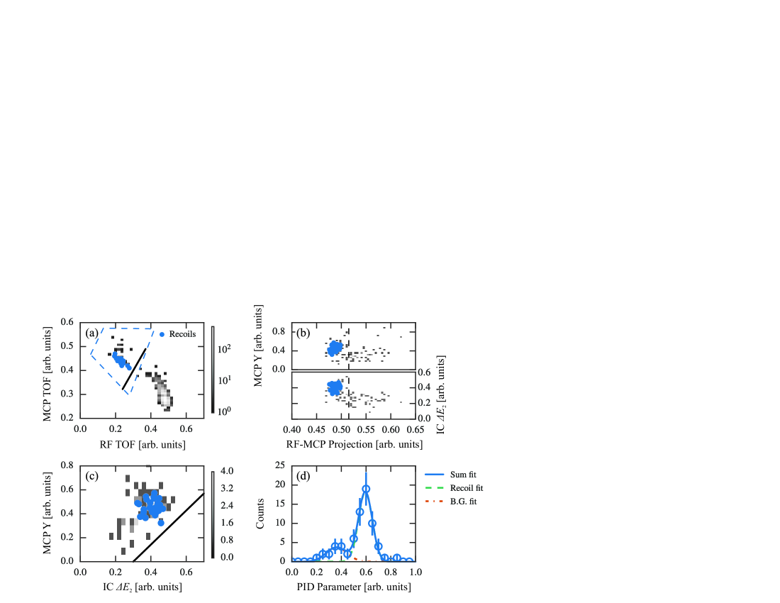
Figure 4: Summary of the singles resonance strength analysis for the $27.17$ MeV beam energy. In panels (a) – (c), the blue filled circles represent events already identified as recoils in the coincidence analysis, and the greyscale intensity maps represent all singles data. In panel (d), the open circles represent all singles data, and the various curves represent fits as indicated in the legend. The solid black lines in panels (a) and (c) represent diagonal axes onto which the two-dimensional data are projected for subsequent analysis. The dashed black lines in panel (b) represent the cut placed on the “RF-MCP Projection” parameter. The full significance of each plot is explained in the main text.

II.3 Singles Analysis

In addition to the coincidence analysis of the $689$ keV resonance presented in Section II.2, we have also performed a separate extraction of the resonance strength using heavy-ion singles data alone. This analysis was guided by the results of the prior coincidence analysis, i.e. regions of interest in various parameter spaces were identified by the location of coincidence recoils. However, the final quantitative cuts applied to the singles data were determined from the distributions of the singles parameters alone. This singles analysis made use of the time difference between the incoming beam bunch (measured from the ISAC-I RFQ signal) and the upstream MCP to construct a separator TOF parameter without requiring prompt $\gamma$ rays. This analysis is summarized in the plots shown in Figure 4. Panel (a) shows the standard MCP TOF signal plotted vs. the RF–MCP TOF, where the 27 events already identified as recoils in the coincidence analysis (represented by the blue filled circles) are tightly clustered in a narrow region of the plot. Continuing the analysis, we first set a gate on the entire upper-left region of the plot, which contains all of the coincidence recoils (the actual gate is included in the Figure 4(a) as the blue dashed line). We then project these events onto the solid black diagonal axis shown in the figure.

The new projected parameter (“RF-MCP projection”) is shown in the panel (b) of Figure 4, plotted vs. two separate parameters: 1) the $y$ position in the upstream MCP, deduced from a resistive-anode readout scheme; and 2) the energy loss in the third (most downstream) anode of the IC. In both cases, the confirmed recoil events are tightly clustered in a single region of the plot. To further separate recoil events from background, we place a one-dimensional cut on the “RF-MCP projection” parameter, including all events to the left of the black dotted line in the figure. For these events only, we then plot the IC energy loss vs. the MCP $y$ position, shown in Figure 4(c). Here, the singles events cluster into two distinct loci, with the confirmed recoil events falling entirely within the upper-right cluster. From this, we conclude that the singles events in the upper-right locus correspond to recoils, while the events in the lower-left locus correspond to background leaky beam events.

To quantify the overlap between the recoil and leaky beam regions in Figure 4(c), we project onto the diagonal axis indicated by the solid black line in the figure. This projection is shown in the Figure 4(d). The measured data (shown as open circles with error bars) are well-described by a double-Gaussian distribution (shown as dashed, dot-dashed, and solid lines, as indicated in the legend). The smaller Gaussian on the left of the figure corresponds to the estimated background distribution, and the larger Gaussian on the right of the figure corresponds to the recoil distribution. We take the true number of recoil events to be equal to the integral of the signal distribution, $52.0\pm 8.2$. The uncertainty on this quantity comes from propagating the $1\sigma$ uncertainties on the individual fit parameters, which were calculated with MINUIT.

To calculate the singles resonance strength, we use the standard thick-target formula Iliadis (2007),

$$\omega\gamma={2N_{r}\epsilon}/({\eta N_{b}\lambda^{2}}),$$ (9)

where $N_{r}=52.0\pm 8.2$ is the number of recoil events, $\epsilon=(3.95\pm 0.14)\times 10^{-15}$ eV cm² is the center-of-mass stopping power, $\eta=0.110\pm 0.003$ is the heavy-ion detection efficiency, $N_{b}=(2.53\pm 0.30)\times 10^{12}$ is the number of beam ions, and $\lambda=(3.513\pm 0.005)\times 10^{-12}$ cm is the center-of-mass deBroglie wavelength. Note that the heavy-ion detection efficiency includes the IC efficiency of $0.913\pm 0.003$. This was not included in the heavy-ion efficiency used in the coincidence analysis since the IC was not used to select coincidence events. The deBroglie wavelength assumes a resonance energy of $E_{r}=679\pm 2$ keV, as extracted from our previous maximum likelihood analysis. The influence of this assumption is minor; calculating the resonance strength using the previous resonance energy of $689\pm 10$ keV increases the result by less than $1$ meV. The resulting resonance strength is $\omega\gamma=120\pm 20$ meV (statistical uncertainty only), which is in good agreement with our coincidence result of $120^{+50}_{-30}$ meV (the exact agreement of the central values should be considered fortuitous). The estimated singles systematic uncertainty is $\pm 15$ meV, calculated by propagating the uncertainties for the stopping power, number of beam particles, and detection efficiency.

In practice, the singles technique frequently results in a lower systematic uncertainty than the coincidence method since there is no need to estimate the $\gamma$-ray detection efficiency. This efficiency typically comes with a relative uncertainty of $10\%$ or greater, resulting from uncertainties in the Geant3 simulation of the BGO array Gigliotti (2004), as well as from unknown $\gamma$-ray decay schemes. However, for reliable application of the singles technique, it is crucial that the full width of the resonance be contained within the gas target, to ensure that the thick-target approximation of the resonance strength formula is valid. In the future, technical advances will likely improve the ability to discern resonance positions based on only a handful of recoil events. With this capability, an off-center resonance would be spotted early on during a running period, and the beam energy could be adjusted accordingly. One example presently under development is the use of a fast-timing LaBr array for $\gamma$-ray detection. The fast timing properties of LaBr allow the resonance position to be deduced from the time difference between the detected $\gamma$ rays and the arrival of the corresponding beam bunch. Preliminary calculations and simulation work suggest that this method is more precise than the presently-employed $z$-position technique and may be applied to data sets with as few as ${\sim}5$ confirmed recoils Ruiz .

III Discussion

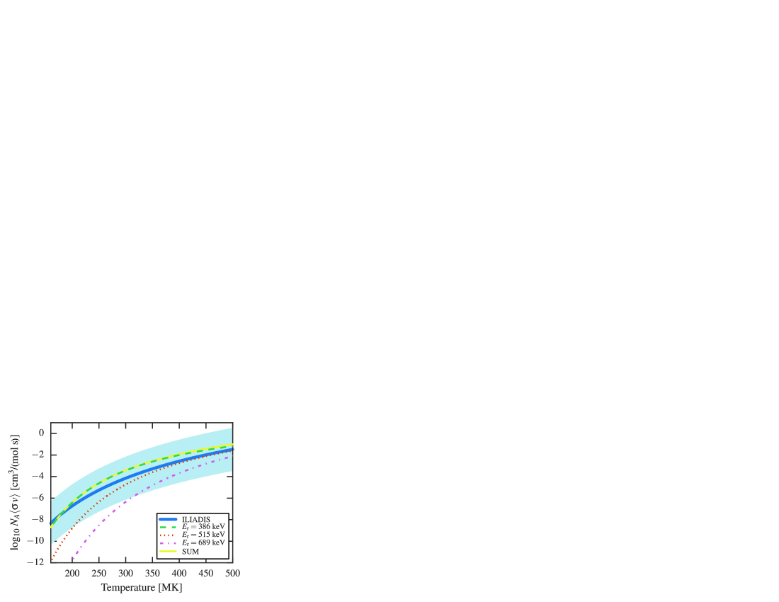
Figure 5: Updated ³⁸K$(p,\gamma)^{39}$Ca reaction rate across the temperature regime covered by classical novae, calculated assuming the rate is dominated by the three $\ell=0$ resonances studied in the present experiment. The contributions of the $386$ and $515$ keV resonances represent upper limits, while the “689 keV” resonance contribution represents our measured central value of $120$ meV. Also shown is the statistical model rate of Ref. Iliadis et al. (2001) (“ILIADIS”), along with its associated uncertainties (shaded region).

Table 4: Calculated abundances for Ar, K, and Ca isotopes, from the NuGrid simulations explained in the text. Results from the Iliadis et al. sensitivity study, model “S1” (as well as model “P2”, for ³⁹K) are included for comparison Iliadis et al. (2002). The quantity $X_{\mathrm{rec}}$ represents the abundance calculated using the recommended ³⁸K$(p,\gamma)^{39}$Ca rate from Ref. Iliadis et al. (2001), while $X_{100}$ and $X_{0.01}$ represent abundances calculated with the recommended rate multiplied by factors of $100$ and $0.01$, respectively. The quantities $X_{\mathrm{up}}$ and $X_{\mathrm{low}}$ represent abundances calculated with the experimental upper and lower limits presented in Ref. Lotay et al. (2016).

Nuclide	$\nicefrac{{X_{\mathrm{100}}}}{{X_{\mathrm{rec}}}}$	$\nicefrac{{X_{\mathrm{up}}}}{{X_{\mathrm{rec}}}}$	$\nicefrac{{X_{\mathrm{low}}}}{{X_{\mathrm{rec}}}}$	$\nicefrac{{X_{\mathrm{0.01}}}}{{X_{\mathrm{rec}}}}$	$\nicefrac{{X_{\mathrm{100}}}}{{X_{\mathrm{0.01}}}}$	$\nicefrac{{X_{\mathrm{up}}}}{{X_{\mathrm{low}}}}$
NuGrid
38Ar	0.066	0.57	1.4	1.4	1/21	1/2.5
39K	3.4	2.1	0.14	0.094	36	15
40Ca	2.4	1.7	0.18	0.069	35	9.4
Iliadis et al. Iliadis et al. (2002)
38Ar (“S1”)	0.057	0.60	1.4	1.4	1/25	1/2.3
39K (“S1”)	3.4	2.0	0.19	0.059	58	11
39K (“P2”)	9.5	2.6	0.17	0.070	136	15
40Ca (“S1”)	2.4	1.7	0.20	0.042	57	8.5

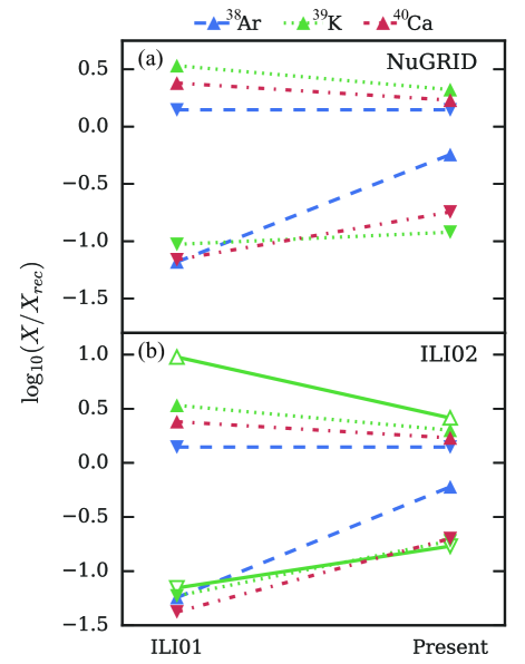
Figure 6: Summary of the sensitivity study results presented in Table 4. The various data points represent the logarithm of the ratio $X/X_{\textrm{rec}}$, where $X_{\textrm{rec}}$ is the predicted abundance of a given isotope taking the recommended ³⁸K$(p,\gamma)^{39}$Ca rate from Ref. Iliadis et al. (2001), and $X$ is the predicted abundance of the same isotope taking the ³⁸K$(p,\gamma)^{39}$Ca rate to be at the upper or lower limit of various uncertainty bands. For the points on the left of the figure (labeled “ILI01”), $X$ is evaluated at the factor of 100 up /0.01 down uncertainty limits given in Ref. Iliadis et al. (2001). For points on the right of the figure (labeled “Present”), $X$ is taken from the uncertainty band established in Ref. Lotay et al. (2016). In all cases, up-turned triangles represent $X$ calculated at the upper limit of the uncertainty band and down-turned triangles represent $X$ at the lower limit. The various dashed, dotted, and dot-dashed lines represent abundance calculations for ³⁸Ar, ³⁹K, and ⁴⁰Ca as indicated in the legend at the top of the figure. Panel (a) shows the results of the present NuGRID sensitivity study, while panel (b) shows the results of the Iliadis et al. sensitivity study Iliadis et al. (2002). In panel (b), results from both the “S1” and “P2” nova models are displayed for ³⁹K. The filled green triangles connected by the dotted line represent results of the “S1” model, while the open triangles connected by solid lines represent the results of the “P2” model.

As discussed in Ref. Lotay et al. (2016), the present measurements place significant constraints on the overall ³⁸K$(p,\gamma)^{39}$Ca reaction rate at nova temperatures. This is demonstrated in Figure 5, which shows the calculated rate vs. temperature curves for the three presently reported resonances, along with their sum. Assuming the astrophysical rate is dominated by these three resonances, the lower curve (the nominal $689$ keV resonance) sets a lower limit on the astrophysical rate, while the sum sets an upper limit. For comparison, the recommended rate from Iliadis et al., along with the factor $100$ up/down uncertainty band, is also included in the figure. At peak temperatures for ONe nova burning, $T\simeq 0.4~{}$GK, the total uncertainty has been reduced from a factor of $10^{4}$ to a factor of ${\sim}40$. Applying these new, experimentally based, limits to the model predictions of the Iliadis et al. sensitivity study Iliadis et al. (2002) results in a reduction of overall uncertainties on ³⁸Ar, ³⁹K, and ⁴⁰Ca production in ONe novae from respective factors of ${\sim}25,$ $136,$ and $57$ to factors of ${\sim}2,$ $18,$ and $9$. Note for these calculations, the nucleosynthesis models which maximized the sensitivity to the ³⁸K$(p,\gamma)^{39}$Ca rate were used. For ³⁸Ar and ⁴⁰Ca this corresponds to the “S1” model ($T_{\mathrm{peak}}=418$ MK), while for ³⁹K the “P2” model ($T_{\mathrm{peak}}=356$ MK) was used.

In order to investigate the dependence of these sensitivity results to specific nova models, we have performed a separate ³⁸K$(p,\gamma)^{39}$Ca sensitivity study based on an independent calculation performed with the NuGrid package, using the single-zone “post processing network” (ppn) code Denissenkov et al. (2014). The initial conditions of the calculation are a $1.3$ solar mass white dwarf with a temperature of $7.0$ MK. The white dwarf composition is given by the “Denisenkov” model, evolved using the Modules for Experiments in Stellar Astrophysics (MESA) code Paxton et al. (2011). The accretion rate is $10^{-11}$ $M_{\odot}/\mathrm{yr}$, and the composition of the accreted material is assumed to be solar. The peak temperature of the model outburst is $408$ MK, similar to the $418$ MK peak temperature of the S1 model from Ref. Iliadis et al. (2002). A complete description of the parameters going into the NuGrid calculation can be found in Ref. Denissenkov et al. (2014). The results of the NuGrid sensitivity study are summarized in Table 4, with results from the Iliadis et al. study included for comparison. The recommended rate utilized for this analysis is identical to the one presented in Ref. Iliadis et al. (2001). Overall, the predictions of the NuGrid and the S1 models are rather consistent, with agreement to within a factor of two in all cases.

Our measurements and sensitivity analyses indicate that the ³⁸K$(p,\gamma)^{39}$Ca rate is not a likely source of significant over- or under-production of ³⁸Ar, ³⁹K or ⁴⁰Ca in novae (relative to solar abundances). Hence the over-production of Ar and Ca observed in the spectra of nova ejecta Pottasch (1959); Andrea et al. (1994); Arkhipova et al. (2000); Evans et al. (2003) remains unexplained. We encourage more extensive sensitivity studies and multi-zone model calculations to investigate the source of this anomaly.

It should be noted that the present results intrinsically depend on the veracity of previous transfer reaction studies, which have established the ³⁹Ca level scheme in the $E_{x}=6$–$7$ MeV region. If the spins or level energies established from these studies are incorrect or incomplete, the present experiment may have neglected to cover the most important resonance energy windows for astrophysics. For this reason, we encourage future high-resolution transfer reaction studies that are targeted specifically at measuring the properties of potential astrophysical proton capture resonances in ³⁹Ca.

Although the present measurements are not directly sensitive to the spins of the measured resonances, we can still infer properties of the resonances in question based on the measured strengths. For this, we use the standard formula for the resonance strength Iliadis (2007),

$$\omega\gamma=\frac{2J_{r}+1}{\left(2J_{p}+1\right)\left(2J_{{}^{38}\mathrm{K}}+1\right)}\frac{\Gamma_{\gamma}\Gamma_{p}}{\Gamma_{\gamma}+\Gamma_{p}},$$ (10)

where $J_{r}=\nicefrac{{5}}{{2}}$, $J_{p}=\nicefrac{{1}}{{2}}$, and $J_{{}^{38}\mathrm{K}}=3$ are the respective spins of the resonance, proton, and ³⁸K; and $\Gamma_{\gamma}$ and $\Gamma_{p}$ are the respective $\gamma$-ray and proton partial widths of the resonance. Assuming a “hard” upper limit on the proton spectroscopic factor for unbound states of $C^{2}S\leq 0.1$ and the measured strength value of $\omega\gamma=120$ meV for the $679\pm 2$ keV resonance, we calculate an upper limit on the mean $\gamma$-decay lifetime for this state of $\tau\leq 2.2$ fs. For shorter lifetimes, as $\tau\rightarrow 0$, $\Gamma_{\gamma}/(\Gamma_{\gamma}+\Gamma_{p})\rightarrow 1$, and we calculate a lower limit on the spectroscopic factor of $C^{2}S\geq 0.0055$. For the $515\pm 10$ keV resonance, the $90\%$ confidence level (CL) upper limit on the strength of $18.4$ meV sets an upper limit on the lifetime of $\tau\leq 12$ fs (again taking the “hard” upper limit on the spectroscopic factor at $C^{2}S=0.1$). For short lifetimes, $\Gamma_{\gamma}/(\Gamma_{\gamma}+\Gamma_{p})\simeq 1$, we calculate an upper limit on the spectroscopic factor of $C^{2}S\leq 0.022$. For the $386\pm 10$ keV resonance, the calculated upper limit on the lifetime is $\tau\leq 38$ fs (again taking the measured $90\%$ upper limit on the strength of $\omega\gamma\leq 2.54$ meV and the “hard” spectroscopic factor limit of $0.1$). For short lifetimes satisfying $\Gamma_{\gamma}/(\Gamma_{\gamma}+\Gamma_{p})\simeq 1$, we calculate an upper limit on the spectroscopic factor of $C^{2}S\leq 0.066$. We emphasize that these limits are simply “back of the envelope” calculations and not intended to set any rigid limits on the single-particle properties of the resonances in question.

To summarize, we have performed the first ever direct measurement of the ³⁸K$(p,\gamma)^{39}$Ca reaction, focusing on the three potential $\ell=0$ resonances within the Gamow Window for classical novae, whose energies have been determined previously to be $386\pm 10$ keV, $515\pm 10$ keV, and $689\pm 10$ keV. For the highest-energy resonance, we observed a clear ³⁹Ca–$\gamma$ coincidence signal consisting of $27$ events. We performed a two-dimensional likelihood analysis on the position distribution of the measured $\gamma$-rays to extract a resonance strength and energy of $\omega\gamma=120^{+50}_{-30}\mathrm{(stat.)}^{+20}_{-60}\mathrm{(sys.)}~{}\mathrm{meV}$ and $E_{r}=679^{+2}_{-1}\mathrm{(stat.)}\pm 1\mathrm{(sys.)}~{}\mathrm{keV}$, respectively. The quoted systematic uncertainties are conservative and include the possibility of background events arising from stable ³⁸Ar beam contamination. We also performed a separate analysis of ³⁹Ca singles data and extracted a resonance strength of $\omega\gamma=120\pm 20\mathrm{(stat.)}\pm 15\mathrm{(sys)}~{}\mathrm{meV}$, consistent with the coincidence result. For the lower two resonances, we observed no events consistent with recoils and used a profile likelihood technique to extract $90\%$ CL upper limits on the resonance strengths of $2.54$ meV and $18.4$ meV for the lower and middle resonances, respectively. Based on these measurements we have established new recommended upper and lower limits for the ³⁸K$(p,\gamma)^{39}$Ca reaction rate which reduce uncertainties at peak nova temperatures ($T_{9}\sim 0.4$) from a factor of $10^{4}$ to a factor ${\sim}40$. Incorporating these new limits into two separate nova model calculations we find that the uncertainties on the predicted abundances of ³⁸Ar, ³⁹K, and ⁴⁰Ca are reduced to a factor of $15$ or below in all cases.