MVG Mechanism: Differential Privacy under Matrix-Valued Query

Abstract.

Differential privacy mechanism design has traditionally been tailored for a scalar-valued query function. Although many mechanisms such as the Laplace and Gaussian mechanisms can be extended to a matrix-valued query function by adding i.i.d. noise to each element of the matrix, this method is often suboptimal as it forfeits an opportunity to exploit the structural characteristics typically associated with matrix analysis. To address this challenge, we propose a novel differential privacy mechanism called the Matrix-Variate Gaussian (MVG) mechanism, which adds a matrix-valued noise drawn from a matrix-variate Gaussian distribution, and we rigorously prove that the MVG mechanism preserves $(\epsilon,\delta)$-differential privacy. Furthermore, we introduce the concept of directional noise made possible by the design of the MVG mechanism. Directional noise allows the impact of the noise on the utility of the matrix-valued query function to be moderated. Finally, we experimentally demonstrate the performance of our mechanism using three matrix-valued queries on three privacy-sensitive datasets. We find that the MVG mechanism can notably outperforms four previous state-of-the-art approaches, and provides comparable utility to the non-private baseline.

1. Introduction

Differential privacy (Dwork et al., 2006a; Dwork et al., 2006b) has become the gold standard for a rigorous privacy guarantee. This has prompted the development of many mechanisms including the classical Laplace mechanism (Dwork et al., 2006b) and the Exponential mechanism (McSherry and Talwar, 2007). In addition, there are other mechanisms that build upon these two classical ones such as those based on data partition and aggregation (Xiao et al., 2011b; Hay et al., 2010; Qardaji et al., 2013b; Li et al., 2014; Zhang et al., 2014; Xiao et al., 2012; Cormode et al., 2012; Qardaji et al., 2013a; Xu et al., 2013; Acs et al., 2012; Nissim et al., 2007), and those based on adaptive queries (Hardt and Rothblum, 2010; Hardt et al., 2012; Li et al., 2010; Li and Miklau, 2012; Yuan et al., 2012; Lyu et al., 2016; Dwork et al., 2010). From this observation, differentially-private mechanisms may be categorized into the basic and derived mechanisms. Privacy guarantee of the basic mechanisms is self-contained, whereas that of the derived mechanisms is achieved through a combination of basic mechanisms, composition theorems, and the post-processing invariance property (Dwork, 2008).

In this work, we design a basic mechanism for matrix-valued queries. Existing basic mechanisms for differential privacy are designed typically for scalar-valued query functions. However, in many practical settings, the query functions are multi-dimensional and can be succinctly represented as matrix-valued functions. Examples of matrix-valued query functions in the real-world applications include the covariance matrix (Dwork et al., 2014; Blum et al., 2005; Chaudhuri et al., 2012), the kernel matrix (Kung, 2014), the adjacency matrix (Godsil and Royle, 2013), the incidence matrix (Godsil and Royle, 2013), the rotation matrix (Hughes et al., 2014), the Hessian matrix (Thacker, 1989), the transition matrix (Gilks et al., 1995), and the density matrix (White, 1992), which find applications in statistics (Friedman et al., 2001), machine learning (Vapnik, 2013), graph theory (Godsil and Royle, 2013), differential equations (Thacker, 1989), computer graphics (Hughes et al., 2014), probability theory (Gilks et al., 1995), quantum mechanics (White, 1992), and many other fields (Wikipedia, 2017).

One property that distinguishes the matrix-valued query functions from the scalar-valued query functions is the relationship and interconnection among the elements of the matrix. One may naively treat these matrices as merely a collection of scalar values, but that could prove suboptimal since the structure and relationship among these scalar values are often informative and essential to the understanding and analysis of the system. For example, in graph theory, the adjacency matrix is symmetric for an undirected graph, but not for a directed graph (Godsil and Royle, 2013) – an observation which is implausible to extract from simply looking at the collection of elements without considering how they are arranged in the matrix.

In differential privacy, the standard method for a matrix-valued query function is to extend a scalar-valued mechanism by adding independent and identically distributed (i.i.d.) noise to each element of the matrix (Dwork et al., 2006b; Dwork et al., 2006a; Dwork and Roth, 2014). However, this method may not be optimal as it fails to utilize the structural characteristics of the matrix-valued noise and query function. Although some advanced methods have explored this possibility in an iterative/procedural manner (Hardt and Rothblum, 2010; Hardt et al., 2012; Nikolov et al., 2013), the structural characteristics of the matrices are still largely under-investigated. This is partly due to the lack of a basic mechanism that is directly designed for matrix-valued query functions, making such utilization and application of available tools in matrix analysis challenging.

In this work, we formalize the study of the matrix-valued differential privacy, and present a new basic mechanism that can readily exploit the structural characteristics of the matrices – the Matrix-Variate Gaussian (MVG) mechanism. The high-level concept of the MVG mechanism is simple – it adds a matrix-variate Gaussian noise scaled to the $L_{2}$-sensitivity of the matrix-valued query function (cf. Fig. 1). We rigorously prove that the MVG mechanism guarantees $(\epsilon,\delta)$-differential privacy. Moreover, due to the multi-dimensional nature of the noise and the query function, the MVG mechanism allows flexibility in the design via the novel notion of directional noise. An important consequence of the concept of directional noise is that the matrix-valued noise in the MVG mechanism can be devised to affect certain parts of the matrix-valued query function less than the others, while providing the same privacy guarantee. In practice, this property could be beneficial as the noise can be tailored to minimally impact the intended utility.

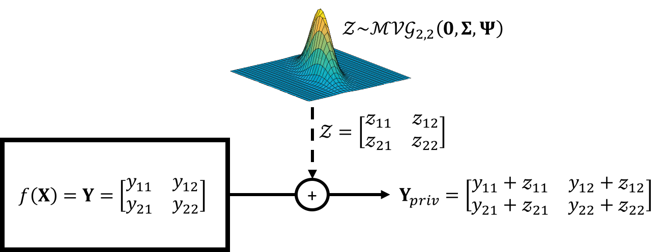
Figure 1. Given a matrix-valued query function $f(\mathbf{X})\in\mathbb{R}^{m\times n}$, the MVG mechanism adds a matrix-valued noise drawn from the matrix-variate Gaussian distribution $\mathcal{MVG}_{m,n}(\mathbf{0},\boldsymbol{\Sigma},\boldsymbol{\Psi})$ to guarantee $(\epsilon,\delta)$-differential privacy. The schematic shows an example when $m=n=2$.

Finally, to illustrate the effectiveness of the MVG mechanism, we conduct experiments on three privacy-sensitive real-world datasets – Liver Disorders (Lichman, 2013; Forsyth and Rada, 1986), Movement Prediction (Bacciu et al., 2014), and Cardiotocography (Lichman, 2013; de Campos et al., 2000). The experiments include three tasks involving matrix-valued query functions – regression, finding the first principal component, and covariance estimation. The results show that the MVG mechanism can outperform four prior state-of-the-art mechanisms – the Laplace mechanism, the Gaussian mechanism, the Exponential mechanism, and the JL transform – in utility in all experiments.

To summarize, our main contributions are as follows.

• We formalize the study of matrix-valued query functions in differential privacy and introduce the novel Matrix-Variate Gaussian (MVG) mechanism.

• We rigorously prove that the MVG mechanism guarantees $(\epsilon,\delta)$-differential privacy.

• We introduce a novel concept of directional noise, and propose two simple algorithms to implement this novel concept with the MVG mechanism.

• We evaluate our approach on three real-world datasets and show that our approach can outperform four prior mechanisms in all experiments, and yields utility close to the non-private baseline.

2. Prior Works

Existing mechanisms for differential privacy may be categorized into two types: the basic mechanism (Dwork et al., 2006b; Dwork et al., 2006a; Blocki et al., 2012; McSherry and Talwar, 2007; Dwork and Roth, 2014; Liu, 2016a; Blum and Roth, 2013; Upadhyay, 2014b, a); and the derived mechanism (Nissim et al., 2007; Johnson et al., 2017; Xiao et al., 2011b; Hay et al., 2010; Qardaji et al., 2013b; Li et al., 2014; Zhang et al., 2014; Xiao et al., 2012; Cormode et al., 2012; Qardaji et al., 2013a; Xu et al., 2013; Acs et al., 2012; Hay et al., 2016; Proserpio et al., 2014; Hardt et al., 2012; Hardt and Rothblum, 2010; Day and Li, 2015; Kenthapadi et al., 2012; Chanyaswad et al., 2017; Xu et al., 2017; Li et al., 2011; Jiang et al., 2013; Li et al., 2010; Li and Miklau, 2012; Hardt and Rothblum, 2010; Dwork et al., 2010; Lyu et al., 2016). Since our work concerns the basic mechanism design, we focus our discussion on this type, and provide a general overview of the other.

2.1. Basic Mechanisms

Basic mechanisms are those whose privacy guarantee is self-contained, i.e. it does not deduce the guarantee from another mechanism. Here, we discuss four popular existing basic mechanisms.

2.1.1. Laplace Mechanism.

The classical Laplace mechanism (Dwork et al., 2006b) adds noise drawn from the Laplace distribution scaled to the $L_{1}$-sensitivity of the query function. It was initially designed for a scalar-valued query function, but can be extended to a matrix-valued query function by adding i.i.d. Laplace noise to each element of the matrix. The Laplace mechanism provides the strong $\epsilon$-differential privacy guarantee and is relatively simple to implement. However, its generalization to a matrix-valued query function does not automatically utilize the structure of the matrices involved.

2.1.2. Gaussian Mechanism.

The Gaussian mechanism (Dwork and Roth, 2014; Dwork et al., 2006a; Liu, 2016a) uses i.i.d. additive noise drawn from the Gaussian distribution scaled to the $L_{2}$-sensitivity. The Gaussian mechanism guarantees $(\epsilon,\delta)$-differential privacy. Like the Laplace mechanism, it also does not automatically consider the structure of the matrices.

2.1.3. Johnson-Lindenstrauss (JL) Transform.

The JL transform method (Blocki et al., 2012) uses multiplicative noise to guarantee $(\epsilon,\delta)$-differential privacy. It is, in fact, a rare basic mechanism designed for a matrix-valued query function. Despite its promise, previous works show that the JL transform method can be applied to queries with certain properties only, e.g.

• Blocki et al. (Blocki et al., 2012) use a random matrix, whose elements are drawn i.i.d. from a Gaussian distribution, and the method is applicable to the Laplacian of a graph and the covariance matrix;

• Blum and Roth (Blum and Roth, 2013) use a hash function that implicitly represents the JL transform, and the method is suitable for a sparse query;

• Upadhyay (Upadhyay, 2014b, a) uses a multiplicative combination of random matrices to provide a JL transform that is applicable to any matrix-valued query function whose singular values are all above a threshold.

Among these methods, Upadhyay’s works (Upadhyay, 2014b, a) stand out as possibly the most general. In our experiments, we show that our approach can yield higher utility for the same privacy budget than these methods.

2.1.4. Exponential Mechanism.

The Exponential mechanism uses noise introduced via the sampling process (McSherry and Talwar, 2007). It draws its query answers from a custom distribution designed to preserve $\epsilon$-differential privacy. To provide reasonable utility, the distribution is chosen based on the quality function, which indicates the utility score of each possible sample. Due to its generality, it has been utilized for many types of query functions, including the matrix-valued query functions. We experimentally compare our approach to the Exponential mechanism, and show that, with slightly weaker privacy guarantee, our method can yield significant utility improvement.

Summary

Finally, we conclude that our method differs from the four existing basic mechanisms as follows. In contrast with the i.i.d. noise in the Laplace and Gaussian mechanisms, the MVG mechanism allows a non-i.i.d. noise (cf. Sec. 5). As opposed to the multiplicative noise in the JL transform and the sampling noise in the Exponential mechanism, the MVG mechanism uses an additive noise for matrix-valued query functions.

2.2. Derived Mechanisms

Derived mechanisms – also referred to as “revised algorithms” by Blocki et al. (Blocki et al., 2012) – are those whose privacy guarantee is deduced from other basic mechanisms via the composition theorems and the post-processing invariance property (Dwork, 2008). Derived mechanisms are often designed to provide better utility by exploiting some properties of the query function or the data.

The general techniques used by derived mechanisms are often translatable among basic mechanisms, including our MVG mechanism. Given our focus on a novel basic mechanism, these techniques are less relevant to our work, and we leave the investigation of integrating them into the MVG framework in the future work, and some of the popular techniques used by derived mechanisms are summarized here.

2.2.1. Sensitivity Control.

This technique avoids the worst-case sensitivity in basic mechanisms by using variant concepts of sensitivity. Examples include the smooth sensitivity (Nissim et al., 2007) and elastic sensitivity (Johnson et al., 2017).

2.2.2. Data Partition and Aggregation.

This technique uses data partition and aggregation to produce more accurate query answers (Xiao et al., 2011b; Hay et al., 2010; Qardaji et al., 2013b; Li et al., 2014; Zhang et al., 2014; Xiao et al., 2012; Cormode et al., 2012; Qardaji et al., 2013a; Xu et al., 2013; Acs et al., 2012). The partition and aggregation processes are done in a differentially-private manner either via the composition theorems and the post-processing invariance property (Dwork, 2008), or with a small extra privacy cost. Hay et al. (Hay et al., 2016) nicely summarize many works that utilize this concept.

2.2.3. Non-uniform Data Weighting.

This technique lowers the level of perturbation required for the privacy protection by weighting each data sample or dataset differently (Proserpio et al., 2014; Hardt et al., 2012; Hardt and Rothblum, 2010; Day and Li, 2015). The rationale is that each sample in a dataset, or each instance of the dataset itself, has a heterogeneous contribution to the query output. Therefore, these mechanisms place a higher weight on the critical samples or instances of the database to provide better utility.

2.2.4. Data Compression.

This approach reduces the level of perturbation required for differential privacy via dimensionality reduction. Various dimensionality reduction methods have been proposed. For example, Kenthapadi et al. (Kenthapadi et al., 2012), Xu et al. (Xu et al., 2017), Li et al. (Li et al., 2011) and Chanyaswad et al. (Chanyaswad et al., 2017) use random projection; Jiang et al. (Jiang et al., 2013) use principal component analysis (PCA) and linear discriminant analysis (LDA); Xiao et al. (Xiao et al., 2011b) use wavelet transform; and Acs et al. (Acs et al., 2012) use lossy Fourier transform.

2.2.5. Adaptive Queries.

These methods use past/auxiliary information to improve the utility of the query answers. Examples are the matrix mechanism (Li et al., 2010; Li and Miklau, 2012), the multiplicative weights mechanism (Hardt and Rothblum, 2010; Hardt et al., 2012), the low-rank mechanism (Yuan et al., 2012, 2015), correlated noise (Nikolov et al., 2013; Xiao et al., 2011a), least-square estimation (Nikolov et al., 2013), boosting (Dwork et al., 2010), and the sparse vector technique (Dwork and Roth, 2014; Lyu et al., 2016). We also note that some of these adaptive methods can be used in the restricted case of matrix-valued query where the matrix-valued query can be decomposed into multiple linear vector-valued queries (Nikolov et al., 2013; Hardt and Talwar, 2010; Yuan et al., 2015; Yuan et al., 2016; Nikolov, 2015; Hardt and Rothblum, 2010). However, such as an approach does not generalize for arbitrary matrix-valued queries.

Summary

We conclude with the following three main observations. (a) First, the MVG mechanism falls into the category of basic mechanism. (b) Second, techniques used in derived mechanisms are generally applicable to multiple basic mechanisms, including our novel MVG mechanism. (c) Finally, therefore, for fair comparison, we will compare the MVG mechanism with the four state-of-the-art basic mechanisms presented in this section.

3. Background

3.1. Matrix-Valued Query

We use the term dataset interchangeably with database, and represent it with the data matrix $\mathbf{X}\in\mathbb{R}^{M\times N}$, whose columns are the $M$-dimensional vector samples/records. The matrix-valued query function, $f(\mathbf{X})\in\mathbb{R}^{m\times n}$, has $m$ rows and $n$ columns . We define the notion of neighboring datasets $\{\mathbf{X}_{1},\mathbf{X}_{2}\}$ as two datasets that differ by a single record, and denote it as $d(\mathbf{X}_{1},\mathbf{X}_{2})=1$. We note, however, that although the neighboring datasets differ by only a single record, $f(\mathbf{X}_{1})$ and $f(\mathbf{X}_{2})$ may differ in every element.

We denote a matrix-valued random variable with the calligraphic font, e.g. $\mathcal{Z}$, and its instance with the bold font, e.g. $\mathbf{Z}$. Finally, as will become relevant later, we use the columns of $\mathbf{X}$ to denote the samples in the dataset.

3.2. $(\epsilon,\delta)$-Differential Privacy

Differential privacy (Dwork, 2006; Dwork et al., 2006a) guarantees that the involvement of any one particular record of the dataset would not drastically change the query answer.

Definition 1.

A mechanism $\mathcal{A}$ on a query function $f(\cdot)$ is $(\epsilon,\delta)$- differentially-private if for all neighboring datasets $\{\mathbf{X}_{1},\mathbf{X}_{2}\}$, and for all possible measurable matrix-valued outputs $\mathbf{S}\subseteq\mathbb{R}^{m\times n}$,

$$\Pr[\mathcal{A}(f(\mathbf{X}_{1}))\in\mathbf{S}]\leq e^{\epsilon}\Pr[\mathcal{A}(f(\mathbf{X}_{2}))\in\mathbf{S}]+\delta.$$

3.3. Matrix-Variate Gaussian Distribution

One of our main innovations is the use of the noise drawn from a matrix-variate probability distribution. Specifically, in the MVG mechanism, the additive noise is drawn from the matrix-variate Gaussian distribution, defined as follows (Dawid, 1981; Gupta and Varga, 1992; Nguyen, 1997; Dutilleul, 1999; Iranmanesh et al., 2010; Waal, 2006).

Definition 2.

An $m\times n$ matrix-valued random variable $\mathcal{X}$ has a matrix-variate Gaussian distribution $\mathcal{MVG}_{m,n}(\mathbf{M},\boldsymbol{\Sigma},\boldsymbol{\Psi})$, if it has the density function:

$$p_{\mathcal{X}}(\mathbf{X})=\frac{\exp\{-\frac{1}{2}\mathrm{tr}[\boldsymbol{\Psi}^{-1}(\mathbf{X}-\mathbf{M})^{T}\boldsymbol{\Sigma}^{-1}(\mathbf{X}-\mathbf{M})]\}}{(2\pi)^{mn/2}\left|\boldsymbol{\Psi}\right|^{m/2}\left|\boldsymbol{\Sigma}\right|^{n/2}},$$

where $\mathrm{tr}(\cdot)$ is the matrix trace (Horn and Johnson, 2012), $\left|\cdot\right|$ is the matrix determinant (Horn and Johnson, 2012), $\mathbf{M}\in\mathbb{R}^{m\times n}$ is the mean, $\boldsymbol{\Sigma}\in\mathbb{R}^{m\times m}$ is the row-wise covariance, and $\boldsymbol{\Psi}\in\mathbb{R}^{n\times n}$ is the column-wise covariance.

Notably, the density function of $\mathcal{MVG}_{m,n}(\mathbf{M},\boldsymbol{\Sigma},\boldsymbol{\Psi})$ looks similar to that of the multivariate Gaussian, $\mathcal{N}_{m}(\boldsymbol{\mu},\boldsymbol{\Sigma})$. Indeed, the matrix-variate Gaussian distribution $\mathcal{MVG}_{m,n}(\mathbf{M},\boldsymbol{\Sigma},\boldsymbol{\Psi})$ is a generalization of $\mathcal{N}_{m}(\boldsymbol{\mu},\boldsymbol{\Sigma})$ to a matrix-valued random variable. This leads to a few notable additions. First, the mean vector $\boldsymbol{\mu}$ now becomes the mean matrix $\mathbf{M}$. Second, in addition to the traditional row-wise covariance matrix $\boldsymbol{\Sigma}$, there is also the column-wise covariance matrix $\boldsymbol{\Psi}$. The latter is due to the fact that, not only could the rows of the matrix be distributed non-uniformly, but also could its columns.

We may intuitively explain this addition as follows. If we draw $n$ i.i.d. samples from $\mathcal{N}_{m}(\mathbf{0},\boldsymbol{\Sigma})$ denoted as $\mathbf{y}_{1},\ldots,\mathbf{y}_{n}\in\mathbb{R}^{m}$, and concatenate them into a matrix $\mathbf{Y}=[\mathbf{y}_{1},\ldots,\mathbf{y}_{n}]\in\mathbb{R}^{m\times n}$, then, it can be shown that $\mathbf{Y}$ is drawn from $\mathcal{MVG}_{m,n}(\mathbf{0},\boldsymbol{\Sigma},\mathbf{I})$, where $\mathbf{I}$ is the identity matrix (Dawid, 1981). However, if we consider the case when the columns of $\mathbf{Y}$ are not i.i.d., and are distributed with the covariance $\boldsymbol{\Psi}$ instead, then, it can be shown that this is distributed according to $\mathcal{MVG}_{m,n}(\mathbf{0},\boldsymbol{\Sigma},\boldsymbol{\Psi})$ (Dawid, 1981).

3.4. Relevant Matrix Algebra Theorems

We recite two major theorems in linear algebra that are essential to the subsequent analysis. The first one is used in multiple parts of the analysis including the privacy proof and the interpretation of the results, while the second one is the concentration bound essential to the privacy proof.

Theorem 1 (Singular value decomposition (SVD) (Horn and Johnson, 2012)).

A matrix $\mathbf{A}\in\mathbb{R}^{m\times n}$ can be decomposed as $\mathbf{A}=\mathbf{W}_{1}\boldsymbol{\Lambda}\mathbf{W}_{2}^{T}$, where $\mathbf{W}_{1}\in\mathbb{R}^{m\times m},\mathbf{W}_{2}\in\mathbb{R}^{n\times n}$ are unitary, and $\boldsymbol{\Lambda}$ is a diagonal matrix whose diagonal elements are the ordered singular values of $\mathbf{A}$, denoted as $\sigma_{1}\geq\sigma_{2}\geq\cdots\geq 0$.

Theorem 2 (Laurent-Massart (Laurent and Massart, 2000)).

For a matrix-variate random variable $\mathcal{N}\sim\mathcal{MVG}_{m,n}(\mathbf{0},\mathbf{I}_{m},\mathbf{I}_{n})$, $\delta\in[0,1]$, and $\zeta(\delta)=2\sqrt{-mn\ln\delta}-2\ln\delta+mn$,

$$\Pr[\left\|\mathcal{N}\right\|_{F}^{2}\leq\zeta(\delta)^{2}]\geq 1-\delta.$$

4. MVG Mechanism: Differential Privacy with Matrix-Valued Query

Matrix-valued query functions are different from their scalar counterparts in terms of the vital information contained in how the elements are arranged in the matrix. To fully exploit these structural characteristics of matrix-valued query functions, we present our novel mechanism for matrix-valued query functions: the Matrix-Variate Gaussian (MVG) mechanism.

First, let us introduce the sensitivity of the matrix-valued query function used in the MVG mechanism.

Definition 3 (Sensitivity).

Given a matrix-valued query function $f(\mathbf{X})\in\mathbb{R}^{m\times n}$, define the $L_{2}$-sensitivity as,

$$s_{2}(f)=\sup_{d(\mathbf{X}_{1},\mathbf{X}_{2})=1}\left\|f(\mathbf{X}_{1})-f(\mathbf{X}_{2})\right\|_{F},$$

where $\left\|\cdot\right\|_{F}$ is the Frobenius norm (Horn and Johnson, 2012).

Then, we present the MVG mechanism as follows.

Definition 4 (MVG mechanism).

Given a matrix-valued query function $f(\mathbf{X})\in\mathbb{R}^{m\times n}$, and a matrix-valued random variable $\mathcal{Z}\sim\mathcal{MVG}_{m,n}(\mathbf{0},\boldsymbol{\Sigma},\boldsymbol{\Psi})$, the MVG mechanism is defined as,

$$\mathcal{MVG}(f(\mathbf{X}))=f(\mathbf{X})+\mathcal{Z},$$

where $\boldsymbol{\Sigma}$ is the row-wise covariance matrix, and $\boldsymbol{\Psi}$ is the column-wise covariance matrix.

So far, we have not specified how to pick $\boldsymbol{\Sigma}$ and $\boldsymbol{\Psi}$ according to the sensitivity $s_{2}(f)$ in the MVG mechanism. We discuss the explicit form of $\boldsymbol{\Sigma}$ and $\boldsymbol{\Psi}$ next.

$\mathbf{X}\in\mathbb{R}^{M\times N}$	database/dataset whose $N$ columns are data samples and $M$ rows are attributes/features.
$\mathcal{MVG}_{m,n}(\mathbf{0},\boldsymbol{\Sigma},\boldsymbol{\Psi})$	$m\times n$ matrix-variate Gaussian distribution with zero mean, the row-wise covariance $\boldsymbol{\Sigma}$, and the column-wise covariance $\boldsymbol{\Psi}$.
$f(\mathbf{X})\in\mathbb{R}^{m\times n}$	matrix-valued query function
$r$	$\min\{m,n\}$
$H_{r}$	generalized harmonic numbers of order $r$
$H_{r,1/2}$	generalized harmonic numbers of order $r$ of $1/2$
$\gamma$	$\sup_{\mathbf{X}}\left\|f(\mathbf{X})\right\|_{F}$
$\zeta(\delta)$	$2\sqrt{-mn\ln\delta}-2\ln\delta+mn$
$\boldsymbol{\sigma}(\boldsymbol{\Sigma}^{-1})$	vector of non-increasing singular values of $\boldsymbol{\Sigma}^{-1}$
$\boldsymbol{\sigma}(\boldsymbol{\Psi}^{-1})$	vector of non-increasing singular values of $\boldsymbol{\Psi}^{-1}$

Table 1. Notations for the differential privacy analysis.

As the additive matrix-valued noise of the MVG mechanism is drawn from $\mathcal{MVG}_{m,n}(\mathbf{0},\boldsymbol{\Sigma},\boldsymbol{\Psi})$, the parameters to be designed for the MVG mechanism are the two covariance matrices $\boldsymbol{\Sigma}$ and $\boldsymbol{\Psi}$. The following theorem presents a sufficient condition for the values of $\boldsymbol{\Sigma}$ and $\boldsymbol{\Psi}$ to ensure that the MVG mechanism preserves $(\epsilon,\delta)$-differential privacy.

Theorem 3.

Let

$$\boldsymbol{\sigma}(\boldsymbol{\Sigma}^{-1})=[\sigma_{1}(\boldsymbol{\Sigma}^{-1}),\ldots,\sigma_{m}(\boldsymbol{\Sigma}^{-1})]^{T},$$

and

$$\boldsymbol{\sigma}(\boldsymbol{\Psi}^{-1})=[\sigma_{1}(\boldsymbol{\Psi}^{-1}),\ldots,\sigma_{n}(\mathbf{\boldsymbol{\Psi}}^{-1})]^{T}$$

be the vectors of non-increasingly ordered singular values of $\boldsymbol{\Sigma}^{-1}$ and $\boldsymbol{\Psi}^{-1}$, respectively, and let the relevant variables be defined according to Table 1. Then, the MVG mechanism guarantees $(\epsilon,\delta)$-differential privacy if $\boldsymbol{\Sigma}$ and $\boldsymbol{\Psi}$ satisfy the following condition,

(1) $$\left\|\boldsymbol{\sigma}(\boldsymbol{\Sigma}^{-1})\right\|_{2}\left\|\boldsymbol{\sigma}(\boldsymbol{\Psi}^{-1})\right\|_{2}\leq\frac{(-\beta+\sqrt{\beta^{2}+8\alpha\epsilon})^{2}}{4\alpha^{2}},$$

where $\alpha=[H_{r}+H_{r,1/2}]\gamma^{2}+2H_{r}\gamma s_{2}(f)$, and $\beta=2(mn)^{1/4}H_{r}s_{2}(f)\zeta(\delta)$.

Proof.

(Sketch) We only provide the sketch proof here. The full proof can be found in Appendix A.

The MVG mechanism guarantees $(\epsilon,\delta)$-differential privacy if for every pair of neighboring datasets $\{\mathbf{X}_{1},\mathbf{X}_{2}\}$ and all measurable sets $\mathbf{S}\subseteq\mathbb{R}^{m\times n}$,

$$\Pr\left[f(\mathbf{X}_{1})+\mathcal{Z}\in\mathbf{S}\right]\leq\exp(\epsilon)\Pr\left[f(\mathbf{X}_{2})+\mathcal{Z}\in\mathbf{S}\right]+\delta.$$

Using Definition 2, this is satisfied if we have,

$$\int_{\mathbf{S}}e^{-\frac{1}{2}\mathrm{tr}[\boldsymbol{\Psi}^{-1}(\mathbf{Y}-f(\mathbf{X}_{1}))^{T}\boldsymbol{\Sigma}^{-1}(\mathbf{Y}-f(\mathbf{X}_{1}))]}d\mathbf{Y}\leq$$

$$e^{\epsilon}\int_{\mathbf{S}}e^{-\frac{1}{2}\mathrm{tr}[\boldsymbol{\Psi}^{-1}(\mathbf{Y}-f(\mathbf{X}_{2}))^{T}\boldsymbol{\Sigma}^{-1}(\mathbf{Y}-f(\mathbf{X}_{2}))]}d\mathbf{Y}+\delta.$$

By inserting $\frac{\exp\{-\frac{1}{2}\mathrm{tr}[\boldsymbol{\Psi}^{-1}(\mathbf{Y}-f(\mathbf{X}_{2}))^{T}\boldsymbol{\Sigma}^{-1}(\mathbf{Y}-f(\mathbf{X}_{2}))]\}}{\exp\{-\frac{1}{2}\mathrm{tr}[\boldsymbol{\Psi}^{-1}(\mathbf{Y}-f(\mathbf{X}_{2}))^{T}\boldsymbol{\Sigma}^{-1}(\mathbf{Y}-f(\mathbf{X}_{2}))]\}}$ inside the integral on the left side, it is sufficient to show that

$$\frac{\exp\{-\frac{1}{2}\mathrm{tr}[\boldsymbol{\Psi}^{-1}(\mathcal{Y}-f(\mathbf{X}_{1}))^{T}\boldsymbol{\Sigma}^{-1}(\mathcal{Y}-f(\mathbf{X}_{1}))]\}}{\exp\{-\frac{1}{2}\mathrm{tr}[\boldsymbol{\Psi}^{-1}(\mathcal{Y}-f(\mathbf{X}_{2}))^{T}\boldsymbol{\Sigma}^{-1}(\mathcal{Y}-f(\mathbf{X}_{2}))]\}}\leq\exp(\epsilon),$$

with probability $\geq 1-\delta$. By algebraic manipulations, we can express this condition as,

$$\mathrm{tr}[\boldsymbol{\Psi}^{-1}\mathcal{Y}^{T}\boldsymbol{\Sigma}^{-1}\boldsymbol{\Delta}+\boldsymbol{\Psi}^{-1}\boldsymbol{\Delta}^{T}\boldsymbol{\Sigma}^{-1}\mathcal{Y}$$

$$+\boldsymbol{\Psi}^{-1}f(\mathbf{X}_{2})^{T}\boldsymbol{\Sigma}^{-1}f(\mathbf{X}_{2})-\boldsymbol{\Psi}^{-1}f(\mathbf{X}_{1})^{T}\boldsymbol{\Sigma}^{-1}f(\mathbf{X}_{1})] \leq 2\epsilon.$$

where $\boldsymbol{\Delta}=f(\mathbf{X}_{1})-f(\mathbf{X}_{2})$. This is the necessary condition that has to be satisfied for all neighboring $\{\mathbf{X}_{1},\mathbf{X}_{2}\}$ with probability $\geq 1-\delta$ for the MVG mechanism to guarantee $(\epsilon,\delta)$-differential privacy. Therefore, we refer to it as the characteristic equation. From here, the proof analyzes the four terms in the sum separately since the trace is additive. The analysis relies on the following lemmas in linear algebra.

Lemma 1 (Merikoski-Sarria-Tarazaga (Merikoski et al., 1994)).

The non-increasingly ordered singular values of a matrix $\mathbf{A}\in\mathbb{R}^{m\times n}$ have the values of $0\leq\sigma_{i}\leq\left\|\mathbf{A}\right\|_{F}/\sqrt{i}$.

Lemma 2 (von Neumann (von Neumann, 1937)).

Let $\mathbf{A},\mathbf{B}\in\mathbb{R}^{m\times n}$; $\sigma_{i}(\mathbf{A})$ and $\sigma_{i}(\mathbf{B})$ be the non-increasingly ordered singular values of $\mathbf{A}$ and $\mathbf{B}$, respectively; and $r=\min\{m,n\}$. Then, $\mathrm{tr}(\mathbf{A}\mathbf{B}^{T})\leq\Sigma_{i=1}^{r}\sigma_{i}(\mathbf{A})\sigma_{i}(\mathbf{B})$.

Lemma 3 (Trace magnitude bound (Horn and Johnson, 1991)).

Let $\sigma_{i}(\mathbf{A})$ be the non-increasingly ordered singular values of $\mathbf{A}\in\mathbb{R}^{m\times n}$, and $r=\min\{m,n\}$. Then, $\left|\mathrm{tr}(\mathbf{A})\right|\leq\sum_{i=1}^{r}\sigma_{i}(\mathbf{A})$.

The proof, then, proceeds with the analysis of each term in the characteristic equation as follows.

The first term: $\mathrm{tr}[\boldsymbol{\Psi}^{-1}\mathcal{Y}^{T}\boldsymbol{\Sigma}^{-1}\boldsymbol{\Delta}]$. Let us denote $\mathcal{Y}=f(\mathbf{X})+\mathcal{Z}$, where $f(\mathbf{X})$ and $\mathcal{Z}$ are any possible instances of the query and the noise, respectively. Then, we can rewrite the first term as, $\mathrm{tr}[\boldsymbol{\Psi}^{-1}f(\mathbf{X})^{T}\boldsymbol{\Sigma}^{-1}\boldsymbol{\Delta}]+\mathrm{tr}[\boldsymbol{\Psi}^{-1}\mathcal{Z}^{T}\boldsymbol{\Sigma}^{-1}\boldsymbol{\Delta}]$. Both parts are then bounded by their singular values via Lemma 2. The singular values are, in turn, bounded via Lemma 1 and Theorem 2 with probability $\geq 1-\delta$. This gives the bound for the first term:

$$\mathrm{tr}[\boldsymbol{\Psi}^{-1}\mathcal{Y}^{T}\boldsymbol{\Sigma}^{-1}\boldsymbol{\Delta}]\leq\gamma H_{r}s_{2}(f)\phi^{2}+(mn)^{1/4}\zeta(\delta)H_{r}s_{2}(f)\phi,$$

where $\phi=(\left\|\boldsymbol{\sigma}(\boldsymbol{\Sigma}^{-1})\right\|_{2}\left\|\boldsymbol{\sigma}(\boldsymbol{\Psi}^{-1})\right\|_{2})^{1/2}$.

The second term: $\mathrm{tr}[\boldsymbol{\Psi}^{-1}\boldsymbol{\Delta}^{T}\boldsymbol{\Sigma}^{-1}\mathcal{Y}]$. By following the same steps as in the first term, the second term has the exact same bound as the first term, i.e.

$$\mathrm{tr}[\boldsymbol{\Psi}^{-1}\boldsymbol{\Delta}^{T}\boldsymbol{\Sigma}^{-1}\mathcal{Y}]\leq\gamma H_{r}s_{2}(f)\phi^{2}+(mn)^{1/4}\zeta(\delta)H_{r}s_{2}(f)\phi.$$

The third term: $\mathrm{tr}[\boldsymbol{\Psi}^{-1}f(\mathbf{X}_{2})^{T}\boldsymbol{\Sigma}^{-1}f(\mathbf{X}_{2})]$. Applying Lemma 2 and Lemma 1, we can readily bound it as,

$$\mathrm{tr}[\boldsymbol{\Psi}^{-1}f(\mathbf{X}_{2})^{T}\boldsymbol{\Sigma}^{-1}f(\mathbf{X}_{2})]\leq\gamma^{2}H_{r}\phi^{2}.$$

The fourth term: $-\mathrm{tr}[\boldsymbol{\Psi}^{-1}f(\mathbf{X}_{1})^{T}\boldsymbol{\Sigma}^{-1}f(\mathbf{X}_{1})]$. Since this term has the negative sign, we use Lemma 3 to bound its magnitude by its singular values. Then, we use Lemma 1 to bound the singular values. This gives the bound for the forth term as,

$$\left|\mathrm{tr}[\boldsymbol{\Psi}^{-1}f(\mathbf{X}_{1})^{T}\boldsymbol{\Sigma}^{-1}f(\mathbf{X}_{1})]\right|\leq\gamma^{2}H_{r,1/2}\phi^{2}.$$

Four terms combined: by combining the four terms and rearranging them, the characteristic equation becomes $\alpha\phi^{2}+\beta\phi\leq 2\epsilon$. This is a quadratic equation, of which the solution is $\phi\in[\frac{-\beta-\sqrt{\beta^{2}+8\alpha\epsilon}}{2\alpha},\frac{-\beta+\sqrt{\beta^{2}+8\alpha\epsilon}}{2\alpha}]$. Since we know $\phi>0$, we have the solution,

$$\phi\leq\frac{-\beta+\sqrt{\beta^{2}+8\alpha\epsilon}}{2\alpha},$$

which implies the criterion in Theorem 3. ∎

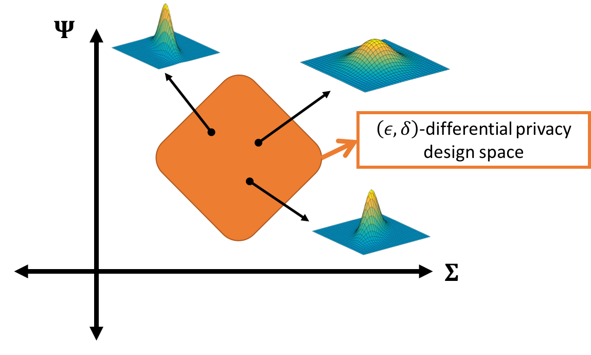
Figure 2. A conceptual display of the MVG design space. The illustration visualizes the design space coordinated by the two design parameters of $\mathcal{MVG}_{m,n}(\mathbf{0},\boldsymbol{\Sigma},\boldsymbol{\Psi})$. Each point on the space corresponds to an instance of $\mathcal{MVG}_{m,n}(\mathbf{0},\boldsymbol{\Sigma},\boldsymbol{\Psi})$. From this perspective, Theorem 3 suggests that any instance of $\mathcal{MVG}_{m,n}(\mathbf{0},\boldsymbol{\Sigma},\boldsymbol{\Psi})$ in the (conceptual) shaded area would preserve $(\epsilon,\delta)$-differential privacy.

Remark 1.

In Theorem 3, we assume that the Frobenius norm of the query function is bounded for all possible datasets by $\gamma$. This assumption is valid in practice because real-world data are rarely unbounded (cf. (Liu, 2016b)), and it is a common assumption in the analysis of differential privacy for multi-dimensional query functions (cf. (Dwork et al., 2006b; Chaudhuri et al., 2012; Zhou et al., 2009; Dwork et al., 2014)).

Remark 2.

The values of the generalized harmonic numbers – $H_{r}$, and $H_{r,1/2}$ – can be obtained from the table lookup for a given value of $r$, or can easily be computed recursively (Sondow and Weisstein, 2017).

The sufficient condition in Theorem 3 yields an important observation: the privacy guarantee of the MVG mechanism depends only on the singular values of $\boldsymbol{\Sigma}$ and $\boldsymbol{\Psi}$. In other words, we may have multiple instances of $\mathcal{MVG}_{m,n}(\mathbf{0},\boldsymbol{\Sigma},\boldsymbol{\Psi})$ that yield the exact same privacy guarantee (cf. Fig. 2). To better understand this phenomenon, in the next section, we introduce the novel concept of directional noise.

5. Directional Noise

Recall from Theorem 3 that the $(\epsilon,\delta)$-differential-privacy condition for the MVG mechanism only applies to the singular values of the two covariance matrices $\boldsymbol{\Sigma}$ and $\boldsymbol{\Psi}$. Here, we investigate the ramification of this result via the novel notion of directional noise.

5.1. Motivation for Non-i.i.d. Noise

For a matrix-valued query function, the standard method for basic mechanisms that use additive noise is by adding the independent and identically distributed (i.i.d.) noise to each element of the matrix query. However, as common in matrix analysis (Horn and Johnson, 2012), the matrices involved often have some geometric and algebraic characteristics that can be exploited. As a result, it is usually the case that only certain “parts” – the term which will be defined more precisely shortly – of the matrices contain useful information. In fact, this is one of the rationales behind many compression techniques such as the popular principal component analysis (PCA) (Kung, 2014; Murphy, 2012; Bishop, 2006). Due to this reason, adding the same amount of noise to every “part” of the matrix query may be highly suboptimal.

5.2. Directional Noise as a Non-i.i.d. Noise

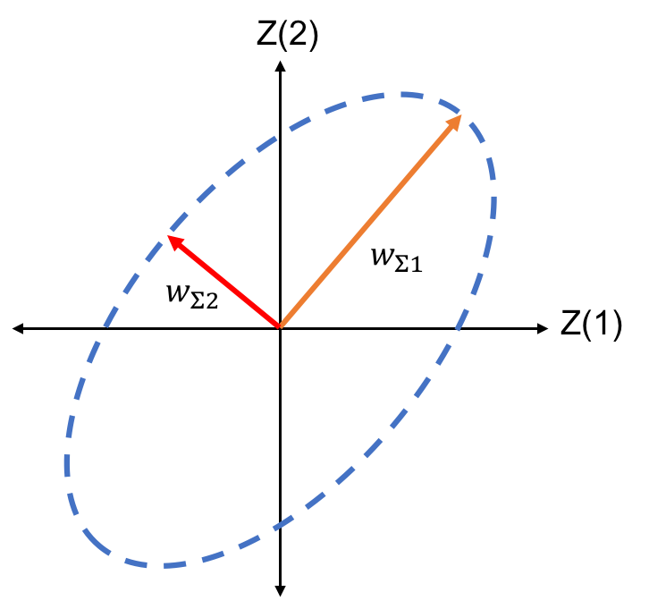
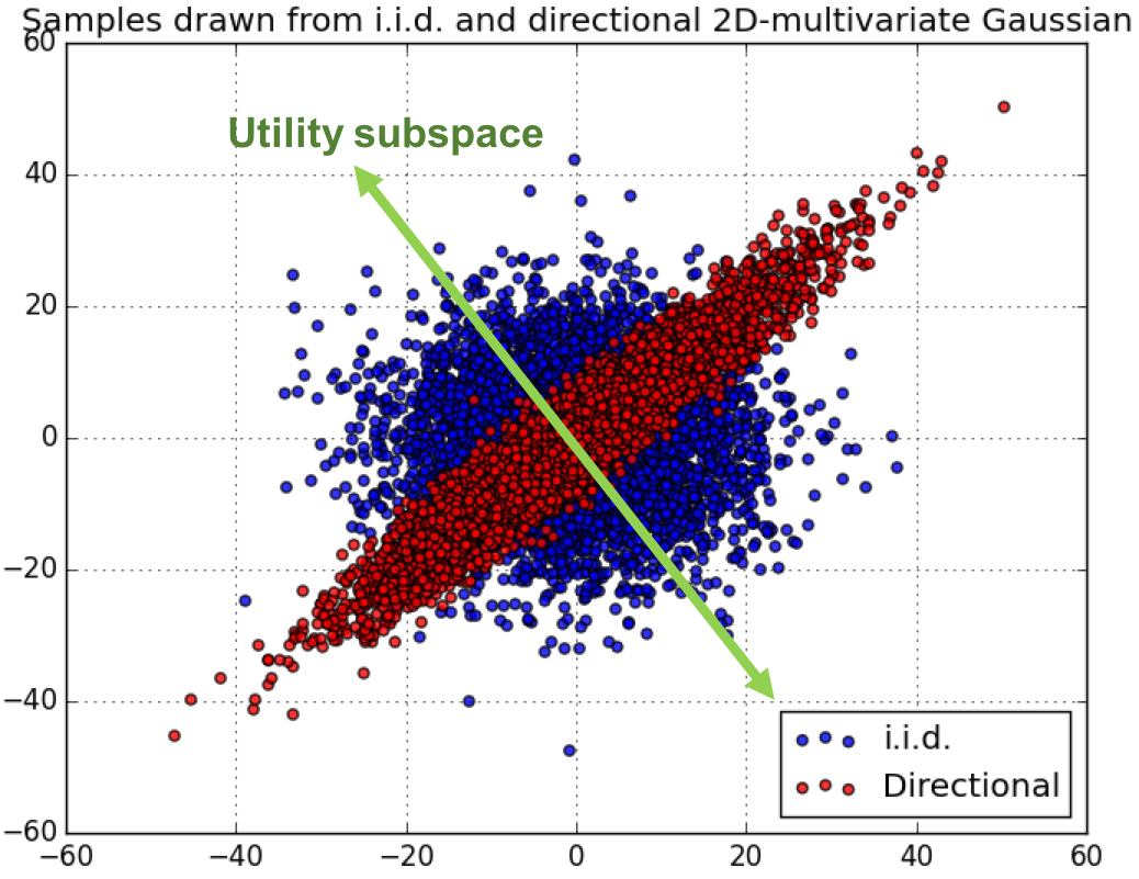
Figure 3. (Left) An ellipsoid of equi-density contour of a 2D multivariate Gaussian distribution. The two arrows indicate the principal axes of this ellipsoid. (Right) Directional noise (red) and i.i.d. noise (blue) drawn from a 2D-multivariate Gaussian distribution. The green line represents a possible utility subspace that can benefit from this instance of directional noise.

Let us elaborate further on the “parts” of a matrix. In matrix analysis, matrix factorization (Horn and Johnson, 2012) is often used to extract underlying properties of a matrix. This is a family of algorithms and the specific choice depends upon the application and types of insights it requires. Particularly, in our application, the factorization that is informative is the singular value decomposition (SVD) (Theorem 1) of the two covariance matrices of $\mathcal{MVG}_{m,n}(\mathbf{0},\boldsymbol{\Sigma},\boldsymbol{\Psi})$.

Consider first the covariance matrix $\boldsymbol{\Sigma}\in\mathbb{R}^{m\times m}$, and write its SVD as, $\boldsymbol{\Sigma}=\mathbf{W}_{1}\boldsymbol{\Lambda}\mathbf{W}_{2}^{T}$. It is well-known that, for the covariance matrix, we have the equality $\mathbf{W}_{1}=\mathbf{W}_{2}$ since it is positive definite (cf. (Abdi, 2007; Horn and Johnson, 2012)). Hence, let us more concisely write the SVD of $\boldsymbol{\Sigma}$ as,

$$\boldsymbol{\Sigma}=\mathbf{W}_{\boldsymbol{\Sigma}}\boldsymbol{\Lambda}_{\boldsymbol{\Sigma}}\mathbf{W}_{\boldsymbol{\Sigma}}^{T}.$$

This representation gives us a very useful insight to the noise generated from $\mathcal{MVG}_{m,n}(\mathbf{0},\boldsymbol{\Sigma},\boldsymbol{\Psi})$: it tells us the directions of the noise via the column vectors of $\mathbf{W}_{\boldsymbol{\Sigma}}$, and variance of the noise in each direction via the singular values in $\boldsymbol{\Lambda}_{\boldsymbol{\Sigma}}$.

For simplicity, consider a two-dimensional multivariate Gaussian distribution, i.e. $m=2$, so there are two column vectors of $\mathbf{W}_{\boldsymbol{\Sigma}}=[\mathbf{w}_{\boldsymbol{\Sigma}1},\mathbf{w}_{\boldsymbol{\Sigma}2}]$. The geometry of this distribution can be depicted by an ellipsoid, e.g. the dash contour in Fig. 3, Left (cf. (Murphy, 2012, ch. 4), (Bishop, 2006, ch. 2)). This ellipsoid is characterized by its two principal axes – the major and the minor axes. It is well-known that the two column vectors from SVD, i.e. $\mathbf{w}_{\boldsymbol{\Sigma}1}$ and $\mathbf{w}_{\boldsymbol{\Sigma}2}$, are unit vectors pointing in the directions of the major and minor axes of this ellipsoid, and more importantly, the length of each axis is characterized by its corresponding singular value, i.e. $\sigma_{\boldsymbol{\Sigma}1}$ and $\sigma_{\boldsymbol{\Sigma}2}$, respectively (cf. (Murphy, 2012, ch. 4)) (recall from Theorem 1 that $diag(\boldsymbol{\Lambda}_{\boldsymbol{\Sigma}})=[\sigma_{\boldsymbol{\Sigma}1},\sigma_{\boldsymbol{\Sigma}2}]$). This is illustrated by Fig. 3, Left. Therefore, when considering this 2D multivariate Gaussian noise, we arrive at the following interpretation of the SVD of its covariance matrix: the noise is distributed toward the two principal directions specified by $\mathbf{w}_{\boldsymbol{\Sigma}1}$ and $\mathbf{w}_{\boldsymbol{\Sigma}2}$, with the variance scaled by the respective singular values, $\sigma_{\boldsymbol{\Sigma}1}$ and $\sigma_{\boldsymbol{\Sigma}2}$.

We can extend this interpretation to a more general case with $m>2$, and also to the other covariance matrix $\boldsymbol{\Psi}$. Then, we have a full interpretation of $\mathcal{MVG}_{m,n}(\mathbf{0},\boldsymbol{\Sigma},\boldsymbol{\Psi})$ as follows. The matrix-valued noise distributed according to $\mathcal{MVG}_{m,n}(\mathbf{0},\boldsymbol{\Sigma},\boldsymbol{\Psi})$ has two components: the row-wise noise, and the column-wise noise. The row-wise noise and the column-wise noise are characterized by the two covariance matrices, $\boldsymbol{\Sigma}$ and $\boldsymbol{\Psi}$, respectively, as follows.

For the row-wise noise.

• The row-wise noise is characterized by $\boldsymbol{\Sigma}$.

• SVD of $\boldsymbol{\Sigma}=\mathbf{W}_{\boldsymbol{\Sigma}}\boldsymbol{\Lambda}_{\boldsymbol{\Sigma}}\mathbf{W}_{\boldsymbol{\Sigma}}^{T}$ decomposes the row-wise noise into two components – the directions and the variances of the noise in those directions.

• The directions of the row-wise noise are specified by the column vectors of $\mathbf{W}_{\boldsymbol{\Sigma}}$.

• The variance of each row-wise-noise direction is indicated by its corresponding singular value in $\boldsymbol{\Lambda}_{\boldsymbol{\Sigma}}$.

For the column-wise noise.

• The column-wise noise is characterized by $\boldsymbol{\Psi}$.

• SVD of $\boldsymbol{\Psi}=\mathbf{W}_{\boldsymbol{\Psi}}\boldsymbol{\Lambda}_{\boldsymbol{\Psi}}\mathbf{W}_{\boldsymbol{\Psi}}^{T}$ decomposes the column-wise noise into two components – the directions and the variances of the noise in those directions.

• The directions of the column-wise noise are specified by the column vectors of $\mathbf{W}_{\boldsymbol{\Psi}}$.

• The variance of each column-wise-noise direction is indicated by its respective singular value in $\boldsymbol{\Lambda}_{\boldsymbol{\Psi}}$.

Since $\mathcal{MVG}_{m,n}(\mathbf{0},\boldsymbol{\Sigma},\boldsymbol{\Psi})$ is fully characterized by its covariances, these two components of the matrix-valued noise drawn from $\mathcal{MVG}_{m,n}(\mathbf{0},\boldsymbol{\Sigma},\boldsymbol{\Psi})$ provide a complete interpretation of the matrix-variate Gaussian noise.

5.3. Directional Noise & MVG Mechanism

We now revisit Theorem 3. Recall that the sufficient $(\epsilon,\delta)$-differential-privacy condition for the MVG mechanism puts the constraint only on the singular values of $\boldsymbol{\Sigma}$ and $\boldsymbol{\Psi}$. However, as we discuss in the previous section, the singular values of $\boldsymbol{\Sigma}$ and $\boldsymbol{\Psi}$ only indicate the variance of the noise in each direction, but not the directions they are attributed to. In other words, Theorem 3 suggests that the MVG mechanism preserves $(\epsilon,\delta)$-differential privacy as long as the overall variances of the noise satisfy a certain threshold, but these variances can be attributed non-uniformly in any direction.

This claim certainly warrants further discussion, and we defer it to Sec. 6, where we present the technical detail on how to practically implement this concept of directional noise. It is important to only note here that this claim does not mean that we can avoid adding noise in any particular direction altogether. On the contrary, there is still a minimum amount of noise required in every direction for the MVG mechanism to guarantee differential privacy, but the noise simply can be attributed unevenly in different directions (see Fig. 3, Right, for an example).

5.4. Utility Gain via Directional Noise

There are multiple ways to exploit the notion of directional noise to enhance utility of differential privacy. Here, we present two methods – via the domain knowledge and via the SVD/PCA.

5.4.1. Utilizing Domain Knowledge

This method is best described by examples. Consider first the personalized warfarin dosing problem (Fredrikson et al., 2014), which can be considered as the regression problem with the identity query, $f(\mathbf{X})=\mathbf{X}$. In the i.i.d. noise scheme, every feature used in the warfarin dosing prediction is equally perturbed. However, domain experts may have prior knowledge that some features are more critical than the others, so adding directional noise designed such that the more critical features are perturbed less can potentially yield better prediction performance.

Let us next consider a slightly more involved matrix-valued query: the covariance matrix, i.e. $f(\mathbf{X})=\frac{1}{N}\mathbf{X}\mathbf{X}^{T}$, where $\mathbf{X}\in\mathbb{R}^{M\times N}$ has zero mean and the columns are the records/samples. Consider now the Netflix prize dataset (Netflix, 2009; Narayanan and Shmatikov, 2008). A popular method for solving the Netflix challenge is via low-rank approximation (Bell et al., 2008), which often involves the covariance matrix query function (Blum et al., 2005; McSherry and Mironov, 2009; Chaudhuri et al., 2012). Suppose domain experts indicate that some features are more informative than the others. Since the covariance matrix has the underlying property that each row and column correspond to a single feature (Murphy, 2012), we can use this domain knowledge with directional noise by adding less noise to the rows and columns corresponding to the informative features.

In both examples, the directions chosen are among the standard basis, e.g. $\mathbf{v}_{1}=[1,0,\ldots,0]^{T},\mathbf{v}_{2}=[0,1,\ldots,0]^{T}$, which are ones of the simplest forms of directions.

5.4.2. Using Differentially-Private SVD/PCA

When domain knowledge is not available, an alternative approach is to derive the directions via the SVD or PCA. In this context, SVD and PCA are identical with the main difference being that SVD is compatible with any matrix-valued query function, while PCA is best suited to the identity query. Hence, the terms may be used interchangeable in the subsequent discussion.

As we show in Sec. 5.2, SVD/PCA can decompose a matrix into its directions and variances. Hence, we can set aside a small portion of privacy budget to derive the directions from the SVD/PCA of the query function. This is illustrated in the following example. Consider again the warfarin dosing problem (Fredrikson et al., 2014), and assume that we do not possess any prior knowledge about the predictive features. We can learn this information from the data by spending a small privacy budget on deriving differentially-private principal components (P.C.). Each P.C. can then serve as a direction and, with directional noise, we can selectively add less noise in the highly informative directions as indicated by PCA.

Clearly, the directions in this example are not necessary among the standard basis, but can be any unit vector. This example illustrates how directional noise can provide additional utility benefit even without the domain knowledge. There have been many works on differentially-private SVD/PCA (Hardt and Roth, 2013a; Kapralov and Talwar, 2013; Blum et al., 2005; Dwork et al., 2014; Chaudhuri et al., 2012; Blocki et al., 2012; Hardt and Roth, 2012, 2013b), so this method is very generally applicable. Again, we reiterate that the approach similar to the one in the example using SVD applies to a general matrix-valued query function. Fig. 3, Right, illustrates this. In the illustration, the query function has two dimensions, and we have obtained the utility direction, e.g. from SVD, as represented by the green line. This can be considered as the utility subspace we desire to be least perturbed. The many small circles in the illustration represent how the i.i.d. noise and directional noise are distributed under the 2D multivariate Gaussian distribution. Clearly, directional noise can reduce the perturbation experienced on the utility directions.

In the next section, we discuss how to implement directional noise with the MVG mechanism in practice and propose two simple algorithms for two types of directional noise.

6. Practical Implementation

The differential privacy condition in Theorem 3, even along with the notion of directional noise in the previous section, still leads to a large design space for the MVG mechanism. In this section, we present two simple algorithms to implement the MVG mechanism with two types of directional noise that can be appropriate for a wide range of real-world applications. Then, we conclude the section with a discussion on a sampling algorithm for $\mathcal{MVG}_{m,n}(\mathbf{0},\boldsymbol{\Sigma},\boldsymbol{\Psi})$.

As discussed in Sec. 5.3, Theorem 3 states that the MVG mechanism satisfies $(\epsilon,\delta)$-differential privacy as long as the singular values of $\boldsymbol{\Sigma}$ and $\boldsymbol{\Psi}$ satisfy the sufficient condition. This provides tremendous flexibility in the choice of the directions of the noise. First, we notice from the sufficient condition in Theorem 3 that the singular values for $\boldsymbol{\Sigma}$ and $\boldsymbol{\Psi}$ are decoupled, i.e. they can be designed independently so long as, when combined, they satisfy the specified condition. Hence, the row-wise noise and column-wise noise can be considered as the two modes of noise in the MVG mechanism. By this terminology, we discuss two types of directional noise: the unimodal and equi-modal directional noise.

6.1. Unimodal Directional Noise

For the unimodal directional noise, we select one mode of the noise to be directional noise, whereas the other mode of the noise is set to be i.i.d. For this discussion, we assume that the row-wise noise is directional noise, while the column-wise noise is i.i.d. However, the opposite case can be readily analyzed with the similar analysis.

We note that, apart from simplifying the practical implementation that we will discuss shortly, this type of directional noise can be appropriate for many applications. For example, for the identity query, we may not possess any prior knowledge on the quality of each sample, so the best strategy would be to consider the i.i.d. column-wise noise (recall that samples are the column vectors).

Formally, the unimodal directional noise sets $\boldsymbol{\Psi}=\mathbf{I}_{n}$, where $\mathbf{I}_{n}$ is the $n\times n$ identity matrix. This, consequently, reduces the design space for the MVG mechanism with directional noise to only that of $\boldsymbol{\Sigma}$. Next, consider the left side of Eq. (1), and we have

(2) $$\left\|\boldsymbol{\sigma}(\boldsymbol{\Sigma}^{-1})\right\|_{2}=\sqrt{\sum_{i=1}^{m}\frac{1}{\sigma_{i}^{2}(\boldsymbol{\Sigma})}}\ \textrm{, and}\ \left\|\boldsymbol{\sigma}(\boldsymbol{\Psi}^{-1})\right\|_{2}=\sqrt{n}.$$

If we square both sides of the sufficient condition and re-arrange it, we get a form of the condition such that the row-wise noise in each direction is decoupled:

(3) $$\sum_{i=1}^{m}\frac{1}{\sigma_{i}^{2}(\boldsymbol{\Sigma})}\leq\frac{1}{n}\frac{(-\beta+\sqrt{\beta^{2}+8\alpha\epsilon})^{4}}{16\alpha^{4}}.$$

This form gives a very intuitive interpretation of the directional noise. First, we note that, to have small noise in the $i^{th}$ direction, $\sigma_{i}(\boldsymbol{\Sigma})$ has to be small (cf. Sec. 5.2). However, the sum of $1/\sigma_{i}^{2}(\boldsymbol{\Sigma})$ of the noise in all directions, which should hence be large, is limited by the quantity on the right side of Eq. (3). This, in fact, explains why even with directional noise, we still need to add noise in every direction to guarantee differential privacy. Consider the case when we set the noise in one direction to be zero, and we have $\underset{\sigma\rightarrow 0}{\lim}\frac{1}{\sigma}=\infty$, which immediately violates the sufficient condition in Eq. (3).

From Eq. (3), the quantity $1/\sigma_{i}^{2}(\boldsymbol{\Sigma})$ is the inverse of the variance of the noise in the $i^{th}$ direction, so we may think of it as the precision measure of the query answer in that direction. The intuition is that the higher this value is, the lower the noise added in that direction, and, hence, the more precise the query value in that direction is. From this description, the constraint in Eq. (3) can be aptly named as the precision budget, and we immediately have the following theorem.

Theorem 4.

For the MVG mechanism with $\boldsymbol{\Psi}=\mathbf{I}_{n}$, the precision budget is $(-\beta+\sqrt{\beta^{2}+8\alpha\epsilon})^{4}/(16\alpha^{4}n)$.

Finally, the remaining task is to determine the directions of the noise and form $\boldsymbol{\Sigma}$ accordingly. To do so systematically, we first decompose $\boldsymbol{\Sigma}$ by SVD as,

$$\boldsymbol{\Sigma}=\mathbf{W}_{\boldsymbol{\Sigma}}\boldsymbol{\Lambda}_{\boldsymbol{\Sigma}}\mathbf{W}_{\boldsymbol{\Sigma}}^{T}.$$

This decomposition represents $\boldsymbol{\Sigma}$ by two components – the directions of the row-wise noise indicated by $\mathbf{W}_{\boldsymbol{\Sigma}}$, and the variance of the noise indicated by $\boldsymbol{\Lambda}_{\boldsymbol{\Sigma}}$. Since the precision budget only puts constraint upon $\boldsymbol{\Lambda}_{\boldsymbol{\Sigma}}$, this decomposition allows us to freely chose any unitary matrix for $\mathbf{W}_{\boldsymbol{\Sigma}}$ such that each column of $\mathbf{W}_{\boldsymbol{\Sigma}}$ indicates each independent direction of the noise.

Therefore, we present the following simple approach to design the MVG mechanism with the unimodal directional noise: under a given precision budget, allocate more precision to the directions of more importance.

Alg. 1 formalizes this procedure. It takes as inputs, among other parameters, the precision allocation strategy $\boldsymbol{\theta}\in(0,1)^{m}$, and the directions $\mathbf{W}_{\boldsymbol{\Sigma}}\in\mathbb{R}^{m\times m}$. The precision allocation strategy is a vector of size $m$, whose elements, $\theta_{i}\in(0,1)$, corresponds to the importance of the $i^{th}$ direction indicated by the $i^{th}$ orthonormal column vector of $\mathbf{W}_{\boldsymbol{\Sigma}}$. The higher the value of $\theta_{i}$, the more important the $i^{th}$ direction is. Moreover, the algorithm enforces that $\sum_{i=1}^{m}\theta_{i}\leq 1$ to ensure that the precision budget is not overspent. The algorithm proceeds as follows. First, compute $\alpha$ and $\beta$ and, then, the precision budget $P$. Second, assign precision to each direction based on the precision allocation strategy. Third, derive the variance of the noise in each direction accordingly. Then, compute $\boldsymbol{\Sigma}$ from the noise variance and directions, and draw a matrix-valued noise from $\mathcal{MVG}_{m,n}(\mathbf{0},\boldsymbol{\Sigma},\mathbf{I})$. Finally, output the query answer with additive matrix noise.

We make a remark here about choosing directions of the noise. As discussed in Sec. 5, any orthonormal set of vectors can be used as the directions. The simplest instance is the the standard basis vectors, e.g. $\mathbf{e}_{1}=[1,0,0]^{T},\mathbf{e}_{2}=[0,1,0]^{T},\mathbf{e}_{3}=[0,0,1]^{T}$ for $\mathbb{R}^{3}$.

Input: (a) privacy parameters: $\epsilon,\delta$; (b) the query function and its sensitivity: $f(\mathbf{X})\in\mathbb{R}^{m\times n},s_{2}(f)$; (c) the precision allocation strategy $\boldsymbol{\theta}\in(0,1)^{m}:\left|\boldsymbol{\theta}\right|_{1}=1$; and (d) the $m$ directions of the row-wise noise $\mathbf{W}_{\boldsymbol{\Sigma}}\in\mathbb{R}^{m\times m}$.

(1) Compute $\alpha$ and $\beta$ (cf. Theorem 3).

(2) Compute the precision budget $P=\frac{(-\beta+\sqrt{\beta^{2}+8\alpha\epsilon})^{4}}{16\alpha^{4}n}$.

(3) for $i=1,\ldots,m$:

i) Set $p_{i}=\theta_{i}P$.

ii) Compute the $i^{th}$ direction’s variance, $\sigma_{i}(\boldsymbol{\Sigma})=1/\sqrt{p_{i}}$.

(4) Form the diagonal matrix $\boldsymbol{\Lambda}_{\boldsymbol{\Sigma}}=diag([\sigma_{1}(\boldsymbol{\Sigma}),\ldots,\sigma_{m}(\boldsymbol{\Sigma})])$.

(5) Derive the covariance matrix: $\boldsymbol{\Sigma}=\mathbf{W}_{\boldsymbol{\Sigma}}\boldsymbol{\Lambda}_{\boldsymbol{\Sigma}}\mathbf{W}_{\boldsymbol{\Sigma}}^{T}$.

(6) Draw a matrix-valued noise $\mathcal{Z}$ from $\mathcal{MVG}_{m,n}(\mathbf{0},\boldsymbol{\Sigma},\mathbf{I})$.

Output: $f(\mathbf{X})+\mathcal{Z}$.

Algorithm 1 MVG mech. w/ unimodal directional noise.

6.2. Equi-Modal Directional Noise

Next, we consider the type of directional noise of which the row-wise noise and column-wise noise are distributed identically, which we call the equi-modal directional noise. We recommend this type of directional noise for a symmetric query function, i.e. $f(\mathbf{X})=f(\mathbf{X})^{T}\in\mathbb{R}^{m\times m}$. This covers a wide-range of query functions including the covariance matrix (Dwork et al., 2014; Blum et al., 2005; Chaudhuri et al., 2012), the kernel matrix (Kung, 2014), the adjacency matrix of an undirected graph (Godsil and Royle, 2013), and the Laplacian matrix (Godsil and Royle, 2013). The motivation for this recommendation is that, for symmetric query functions, any prior information about the rows would similarly apply to the columns, so it is reasonable to use identical row-wise and column-wise noise.

Formally, this type of directional noise imposes that $\boldsymbol{\Psi}=\boldsymbol{\Sigma}$. Following a similar derivation to the unimodal type, we have the following precision budget.

Theorem 5.

For the MVG mechanism with $\boldsymbol{\Psi}=\boldsymbol{\Sigma}$, the precision budget is $(-\beta+\sqrt{\beta^{2}+8\alpha\epsilon})^{2}/(4\alpha^{2})$.

Following a similar procedure to the unimodal type, we present Alg. 2 for the MVG mechanism with the equi-modal directional noise. The algorithm follows the same steps as Alg. 1, except it derives the precision budget from Theorem 5, and draws the noise from $\mathcal{MVG}_{m,m}(\mathbf{0},\boldsymbol{\Sigma},\boldsymbol{\Sigma})$.

Input: (a) privacy parameters: $\epsilon,\delta$; (b) the query function and its sensitivity: $f(\mathbf{X})\in\mathbb{R}^{m\times m},s_{2}(f)$; (c) the precision allocation strategy $\boldsymbol{\theta}\in(0,1)^{m}:\left|\boldsymbol{\theta}\right|_{1}=1$; and (d) the $m$ noise directions $\mathbf{W}_{\boldsymbol{\Sigma}}\in\mathbb{R}^{m\times m}$.

(1) Compute $\alpha$ and $\beta$ (cf. Theorem 3).

(2) Compute the precision budget $P=\frac{(-\beta+\sqrt{\beta^{2}+8\alpha\epsilon})^{2}}{4\alpha^{2}}$.

(3) for $i=1,\ldots,m$:

i) Set $p_{i}=\theta_{i}P$.

ii) Compute the the $i^{th}$ direction’s variance, $\sigma_{i}(\boldsymbol{\Sigma})=1/\sqrt{p_{i}}$.

(4) Form the diagonal matrix $\boldsymbol{\Lambda}_{\boldsymbol{\Sigma}}=diag([\sigma_{1}(\boldsymbol{\Sigma}),\ldots,\sigma_{m}(\boldsymbol{\Sigma})])$.

(5) Derive the covariance matrix: $\boldsymbol{\Sigma}=\mathbf{W}_{\boldsymbol{\Sigma}}\boldsymbol{\Lambda}_{\boldsymbol{\Sigma}}\mathbf{W}_{\boldsymbol{\Sigma}}^{T}$.

(6) Draw a matrix-valued noise $\mathcal{Z}$ from $\mathcal{MVG}_{m,m}(\mathbf{0},\boldsymbol{\Sigma},\boldsymbol{\Sigma})$.

Output: $f(\mathbf{X})+\mathcal{Z}$.

Algorithm 2 MVG mech. w/ equi-modal directional noise.

6.3. Sampling from $\mathcal{MVG}_{m,n}(\mathbf{0},\boldsymbol{\Sigma},\boldsymbol{\Psi})$

One remaining question on the practical implementation of the MVG mechanism is how to efficiently draw the noise from the matrix-variate Gaussian distribution $\mathcal{MVG}_{m,n}(\mathbf{0},\boldsymbol{\Sigma},\boldsymbol{\Psi})$. One approach to implement a sampler for $\mathcal{MVG}_{m,n}(\mathbf{0},\boldsymbol{\Sigma},\boldsymbol{\Psi})$ is via the affine transformation of samples drawn i.i.d. from the standard normal distribution, i.e. $\mathcal{N}(0,1)$. The transformation is described by the following lemma (Dawid, 1981).

Lemma 4.

Let $\mathcal{N}\in\mathbb{R}^{m\times n}$ be a matrix-valued random variable whose elements are drawn i.i.d. from the standard normal distribution $\mathcal{N}(0,1)$. Then, the matrix $\mathcal{Z}=\mathbf{B}_{\boldsymbol{\Sigma}}\mathcal{N}\mathbf{B}_{\boldsymbol{\Psi}}^{T}$ is distributed according to $\mathcal{Z}\sim\mathcal{MVG}_{m,n}(\mathbf{0},\mathbf{B}_{\boldsymbol{\Sigma}}\mathbf{B}_{\boldsymbol{\Sigma}}^{T},\mathbf{B}_{\boldsymbol{\Psi}}\mathbf{B}_{\boldsymbol{\Psi}}^{T})$.

This transformation consequently allows the conversion between $mn$ samples drawn i.i.d. from $\mathcal{N}(0,1)$ and a sample drawn from $\mathcal{MVG}_{m,n}(\mathbf{0},\mathbf{B}_{\boldsymbol{\Sigma}}\mathbf{B}_{\boldsymbol{\Sigma}}^{T},\mathbf{B}_{\boldsymbol{\Psi}}\mathbf{B}_{\boldsymbol{\Psi}}^{T})$. To derive $\mathbf{B}_{\boldsymbol{\Sigma}}$ and $\mathbf{B}_{\boldsymbol{\Psi}}$ from given $\boldsymbol{\Sigma}$ and $\boldsymbol{\Psi}$ for $\mathcal{MVG}_{m,n}(\mathbf{0},\boldsymbol{\Sigma},\boldsymbol{\Psi})$, we solve the two linear equations: $\mathbf{B}_{\boldsymbol{\Sigma}}\mathbf{B}_{\boldsymbol{\Sigma}}^{T}=\boldsymbol{\Sigma}$, and $\mathbf{B}_{\boldsymbol{\Psi}}\mathbf{B}_{\boldsymbol{\Psi}}^{T}=\boldsymbol{\Psi}$, and the solutions of these two equations can be acquired readily via the Cholesky decomposition or SVD (cf. (Horn and Johnson, 2012)). We summarize the steps for this implementation here using SVD:

1. Draw $mn$ i.i.d. samples from $\mathcal{N}(0,1)$, and form a matrix $\mathcal{N}$.

2. Let $\mathbf{B}_{\boldsymbol{\Sigma}}=\mathbf{W}_{\boldsymbol{\Sigma}}\boldsymbol{\Lambda}_{\boldsymbol{\Sigma}}^{1/2}$ and $\mathbf{B}_{\boldsymbol{\Psi}}=\mathbf{W}_{\boldsymbol{\Psi}}\boldsymbol{\Lambda}_{\boldsymbol{\Psi}}^{1/2}$, where $\mathbf{W}_{\boldsymbol{\Sigma}},\boldsymbol{\Lambda}_{\boldsymbol{\Sigma}}$ and $\mathbf{W}_{\boldsymbol{\Psi}},\boldsymbol{\Lambda}_{\boldsymbol{\Psi}}$ are derived from SVD of $\boldsymbol{\Sigma}$ and $\boldsymbol{\Psi}$, respectively.

3. Compute the sample $\mathcal{Z}=\mathbf{B}_{\boldsymbol{\Sigma}}\mathcal{N}\mathbf{B}_{\boldsymbol{\Psi}}^{T}$.

The complexity of this method depends on that of the $\mathcal{N}(0,1)$ sampler used. Plus, there is an additional $\mathcal{O}(\max\{m^{3},n^{3}\})$ complexity from SVD (Golub and Loan, 1996). The memory needed is in the order of $m^{2}+n^{2}+mn$ from the three matrices required in step (3).

7. Experimental Setups

We evaluate the proposed MVG mechanism on three experimental setups and datasets. Table 2 summarizes our setups. In all experiments, 100 trials are carried out and the average and 95% confidence interval are reported.

7.1. Experiment I: Regression

7.1.1. Task and Dataset.

The first experiment considers the regression application on the Liver Disorders dataset (Lichman, 2013; McDermott and Forsyth, 2016), which contains 5 features from the blood sample of 345 patients. We leave out the samples from 97 patients for testing, so the private dataset contains 248 patients. Following suggestions by Forsyth and Rada (Forsyth and Rada, 1986), we use these features to predict the average daily alcohol consumption. All features and teacher values are $\in[0,1]$.

7.1.2. Query Function and Evaluation Metric.

We perform regression in a differentially-private manner via the identity query, i.e. $f(\mathbf{X})=\mathbf{X}$. Since regression involves the teacher values, we treat them as a feature, so the query size becomes $6\times 248$. We use the kernel ridge regression (KRR) (Kung, 2014; Pedregosa et al., 2011) as the regressor, and the root-mean-square error (RMSE) (Murphy, 2012; Kung, 2014) as the evaluation metric.

7.1.3. MVG Mechanism Design.

As discussed in Sec. 6.1, Alg. 1 is appropriate for the identity query, so we employ it for this experiment. The $L_{2}$-sensitivity of this query is $\sqrt{6}$ (cf. Appendix B). To identify the informative directions to allocate the precision budget, we implement both methods discussed in Sec. 5.4 as follows.

(a) For the method using domain knowledge (denoted MVG-1), we refer to Alatalo et al. (Alatalo et al., 2008), which indicates that alanine aminotransferase (ALT) is the most indicative feature for predicting the alcohol consumption behavior. Additionally, from our prior experience working with regression problems, we anticipate that the teacher value (Y) is another important feature to allocate more precision budget to. With this setup, we use the standard basis vectors as the directions (cf. Sec. 5.4), and employ the following binary precision allocation strategy.

• Allocate $\tau$% of the precision budget to the two important features (ALT and Y) by equal amount.

• Allocate the rest of the precision budget equally to the rest of the features.

We vary $\tau\in\{55,65,\ldots,95\}$ and report the best results.

(b) For the method using differentially-private SVD/PCA (denoted MVG-2), given the total budget of $\{\epsilon,\delta\}$ reported in Sec. 8, we spend $0.2\epsilon$ and $0.2\delta$ on the derivation of the two most informative directions via the differentially-private PCA algorithm in (Blum et al., 2005). We specify the first two principal components as the indicative features for a fair comparison with the method using domain knowledge. The remaining $0.8\epsilon$ and $0.8\delta$ are then used for Alg. 1. Again, for a fair comparison with the method using domain knowledge, we use the same binary precision allocation strategy in Alg. 1 for MVG-2.

7.2. Experiment II: 1^st Principal Component

	Exp. I	Exp. II	Exp. III
Task	Regression	$1^{st}$ P.C.	Covariance estimation
Dataset	Liver (Lichman, 2013; Forsyth and Rada, 1986)	Movement (Bacciu et al., 2014)	CTG (Lichman, 2013; de Campos et al., 2000)
# samples $N$	248	2,021	2,126
# features $M$	6	4	21
Query $f(\mathbf{X})$	$\mathbf{X}$	$\mathbf{X}\mathbf{X}^{T}/N$	$\mathbf{X}$
Query size	$6\times 248$	$4\times 4$	$21\times 2126$
Eval. metric	RMSE	$\Delta\rho$ (Eq. (4))	RSS (Eq. (5))
MVG Alg.	1	2	1
Source of directions	Domain knowledge (Alatalo et al., 2008) /PCA (Blum et al., 2005)	Data collection setup (Bacciu et al., 2014)	Domain knowledge (Santos et al., 2006)

Table 2. The three experimental setups.

7.2.1. Task and Dataset.

The second experiment considers the problem of determining the first principal component ($1^{st}$ P.C.) from the principal component analysis (PCA). This is one of the most popular problems in machine learning and differential privacy. We only consider the first principal component for two reasons. First, many prior works in differentially-private PCA algorithm consider this problem or the similar problem of deriving a few major P.C. (cf. (Chaudhuri et al., 2012; Blocki et al., 2012; Dwork et al., 2014)), so this allows us to compare our approach to the state-of-the-art approaches of a well-studied problem. Second, in practice, this method for deriving the $1^{st}$ P.C. may be used iteratively to derive the rest of the principal components (cf. (Jolliffe, 1986)).

We use the Movement Prediction via RSS (Movement) dataset (Bacciu et al., 2014), which consists of the radio signal strength measurement from 4 sensor anchors (ANC{0-3}) – corresponding to the 4 features – from 2,021 movement samples. The feature data all have the range of $[-1,1]$.

7.2.2. Query Function and Evaluation Metric.

We consider the covariance matrix query, i.e. $f(\mathbf{X})=\frac{1}{N}\mathbf{X}\mathbf{X}^{T}$, and use SVD to derive the $1^{st}$ P.C. from it. Hence, the query size is $4\times 4$. We adopt the quality metric commonly used for P.C. (Kung, 2014) and also used by Dwork et al. (Dwork et al., 2014), i.e. the captured variance $\rho$. For a given P.C. $\mathbf{v}$, the capture variance by $\mathbf{v}$ on the covariance matrix $\bar{\mathbf{S}}$ is defined as $\rho=\mathbf{v}^{T}\bar{\mathbf{S}}\mathbf{v}$. To be consistent with other experiments, we report the absolute error in $\rho$ as deviated from the maximum $\rho$. It is well-established that the maximum $\rho$ is equal to the largest eigenvalue of $\bar{\mathbf{S}}$ (cf. (Horn and Johnson, 2012, Theorem 4.2.2), (Rao, 1964)). Hence, the metric can be written as,

(4) $$\Delta\rho(\mathbf{v})=\lambda_{1}-\rho(\mathbf{v}),$$

where $\lambda_{1}$ is the largest eigenvalue of $\bar{\mathbf{S}}$. For the ideal, non-private case, the error would clearly be zero.

7.2.3. MVG Mechanism Design.

As discussed in Sec. 6.2, Alg. 2 is appropriate for the covariance query, so we employ it for this experiment. The $L_{2}$-sensitivity of this query is $8/2021$ (cf. Appendix B). To identify the informative directions to allocate the precision budget, we inspect the data collection setup described in (Bacciu et al., 2014), and use two of the four anchors as the more informative anchors due to their proximity to the movement path (ANC0 and ANC3). Hence, we use the standard basis vectors as the directions (cf. Sec. 6) and allocate more precision budget to these two features using the same strategy as in Exp. I.

7.3. Experiment III: Covariance Estimation

7.3.1. Task and Dataset.

The third experiment considers the similar problem to Exp. II but with a different flavor. In this experiment, we consider the task of estimating the covariance matrix from the perturbed database. This differs from Exp. II in three ways. First, for covariance estimation, we are interested in every P.C. Second, as mentioned in Exp. II, many previous works do not consider every P.C., so the previous works for comparison are different. Third, to give a different taste of our approach, we consider the method of input perturbation for estimating the covariance, i.e. query the noisy database and use it to compute the covariance. We use the Cardiotocography (CTG) dataset (Lichman, 2013; de Campos et al., 2000), which consists of 21 features in the range of $[0,1]$ from 2,126 fetal samples.

7.3.2. Query Function and Evaluation Metric.

We consider the method via input perturbation, so we use the identity query, i.e. $f(\mathbf{X})=\mathbf{X}$. The query size is $21\times 2126$. We adopt the captured variance as the quality metric similar to Exp. II, but since we are interested in every P.C., we consider the residual sum of square (RSS) (Friedman et al., 2001) of every P.C. This is similar to the total residual variance used by Dwork et al. ((Dwork et al., 2014, p. 5)). Formally, given the perturbed database $\tilde{\mathbf{X}}$, the covariance estimate is $\tilde{\mathbf{S}}=\frac{1}{N}\tilde{\mathbf{X}}\tilde{\mathbf{X}}^{T}$. Let $\{\tilde{\mathbf{v}}_{i}\}$ be the set of P.C.’s derived from $\tilde{\mathbf{S}}$, and the RSS is,

(5) $$RSS(\tilde{\mathbf{S}})=\sum_{i}(\lambda_{i}-\rho(\tilde{\mathbf{v}}_{i}))^{2},$$

where $\lambda_{i}$ is the $i^{th}$ eigenvalue of $\bar{\mathbf{S}}$ (cf. Exp. II), and $\rho(\tilde{\mathbf{v}}_{i})$ is the captured variance of the $i^{th}$ P.C. derived from $\tilde{\mathbf{S}}$. Clearly, in the non-private case, $RSS(\bar{\mathbf{S}})=0$.

7.3.3. MVG Mechanism Design.

Since we consider the identity query, we employ Alg. 1 for this experiment. The $L_{2}$-sensitivity is $\sqrt{21}$ (cf. Appendix B). To identify the informative directions to allocate the precision budget to, we refer to the domain knowledge from Costa Santos et al. (Santos et al., 2006), which identifies three features to be most informative, viz. fetal heart rate (FHR), %time with abnormal short term variability (ASV), and %time with abnormal long term variability (ALV). Hence, we use the standard basis vectors as the directions and allocate more precision budget to these three features using the same strategy as in Exp. I.

7.4. Comparison to Previous Works

Since our approach falls into the category of basic mechanism, we compare our work to the four prior state-of-the-art basic mechanisms discussed in Sec. 2.1, namely, the Laplace mechanism, the Gaussian mechanism, the Exponential mechanism, and the JL transform method.

For Exp. I and III, since we consider the identity query, the four previous works for comparison are by Dwork et al. (Dwork et al., 2006b), Dwork et al. (Dwork et al., 2006a), Blum et al. (Blum et al., 2013), and Upadhyay (Upadhyay, 2014a), for the four basic mechanisms, respectively.

For Exp. II, we consider the $1^{st}$ P.C. As this problem has been well-investigated, we compare our approach to the state-of-the-art algorithms specially designed for this problem. These four algorithms using the four prior basic mechanisms are, respectively: Dwork et al. (Dwork et al., 2006b), Dwork et al. (Dwork et al., 2014), Chaudhuri et al. (Chaudhuri et al., 2012), and Blocki et al. (Blocki et al., 2012). We note that these four algorithms chosen for comparison are designed and optimized specifically for the particular application, so they utilize the positive-semidefinite (PSD) nature of the matrix query. On the other hand, the MVG mechanism used here is generally applicable for matrix queries even beyond the particular application, and makes no assumptions about the PSD structure of the matrix query. In other words, we intentionally give a favorable edge to the compared methods to show that, despite the handicap, the MVG mechanism can still perform comparably well.

For all previous works, we use the parameter values as suggested by the authors of the method, and vary the free variable before reporting the best performance.

Finally, we recognize that some of these prior works have a different privacy guarantee from ours, namely, $\epsilon$-differential privacy. Nevertheless, we present these prior works for comprehensive coverage of prior basic mechanisms, and we will keep this difference in mind when discussing the results.

8. Experimental Results

Table 3, Table 4, and Table 5 report the experimental results for Experiment I, II, and III, respectively. The performance shown is an average over 100 trials, along with the 95% confidence interval.

Method	$\epsilon$	$\delta$	RMSE ($\times 10^{-2}$)
Non-private	-	-	1.226
Random guess	-	-	$\sim 3.989$
MVG-1 (Alg. 1 + knowledge in (Alatalo et al., 2008))	1.	$1/N$	$1.624\pm 0.026$
MVG-2 (Alg. 1 + DP-PCA (Blum et al., 2005))	1.	$1/N$	$1.643\pm 0.023$
Gaussian (Dwork et al. (Dwork et al., 2006a))	1.	$1/N$	$1.913\pm 0.069$
JL transform (Upadhyay (Upadhyay, 2014a))	1.	$1/N$	$1.682\pm 0.015$
Laplace (Dwork et al. (Dwork et al., 2006b))	1.	0	$2.482\pm 0.189$
Exponential (Blum et al. (Blum et al., 2013))	1.	0	$2.202\pm 0.721$

Table 3. Results from Exp. I: regression. MVG-1 derives noise directions from domain knowledge, while MVG-2 derives them from differentially-private PCA in (Blum et al., 2005).

8.1. Experiment I: Regression

Table 3 reports the results for Exp. I. Here are the key observations.

• Compared to the non-private baseline, the best MVG mechanism (MVG-1) yields similar performance (difference of .004 in RMSE).

• Compared to other $(\epsilon,\delta)$-basic mechanisms, i.e. the Gaussian mechanism and the JL transform, the best MVG mechanism (MVG-1) has better utility (by .003 and .0006 in RMSE, respectively) with the same privacy guarantee.

• Compared to other $\epsilon$-basic mechanisms, i.e. the Laplace and Exponential mechanisms, the best MVG mechanism (MVG-1) provides significantly better utility (~150%) with the slightly weaker $(\epsilon,1/N)$-differential privacy guarantee.

• Even when some privacy budget is spent on deriving the direction via PCA(Blum et al., 2005) (MVG-2), the MVG mechanism still yields the best performance among all other non-MVG methods.

Overall, the results from regression show the promise of the MVG mechanism. Our approach can outperform all other $(\epsilon,\delta)$-basic mechanisms. Although it provides a weaker privacy guarantee than other $\epsilon$-basic mechanisms, it can provide considerably more utility (~150%). As advocated by Duchi et al. (Duchi et al., 2013) and Fienberg et al. (Fienberg et al., 2010), this trade-off could be attractive in some settings, e.g. critical medical or emergency situations.

8.2. Experiment II: 1^st Principal Component

Method	$\epsilon$	$\delta$	Err. $\Delta\rho$ ($\cdot 10^{-1})$
Non-private	-	-	$0$
Random guess	-	-	$\sim 3.671$
MVG (Alg. 2)	1.	$1/N$	$2.384\pm 0.215$
Gaussian (Dwork et al. (Dwork et al., 2014))	1.	$1/N$	$2.485\pm 0.207$
JL transform (Blocki et al. (Blocki et al., 2012))	1.	$1/N$	$2.394\pm 0.216$
Laplace (Dwork et al. (Dwork et al., 2006b))	1.	0	$2.634\pm 0.174$
Exponential (Chaudhuri et al. (Chaudhuri et al., 2012))	1.	0	$2.455\pm 0.209$

Table 4. Results from Exp. II: first principal component.

Table 4 reports the results for Exp. II. Here are the key observations.

• Compared to the non-private baseline, the MVG mechanism has reasonably small error $\Delta\rho$ of $0.2387$.

• Compared to other $(\epsilon,\delta)$-basic mechanisms, i.e. the Gaussian mechanism and the JL transform, the MVG mechanism provides better utility with the same privacy guarantee (.01 and .0001 smaller error $\Delta\rho$, respectively).

• Compared to other $\epsilon$-basic mechanisms, i.e. the Laplace and Exponential mechanisms, the MVG mechanism yields higher utility with slightly weaker $(\epsilon,1/N)$-differential privacy guarantee (.03 and .01 smaller error $\Delta\rho$, respectively).

Overall, the MVG mechanism provides the best utility. Though we admit that, with a weaker privacy guarantee, it does not provide significant utility increase over the Exponential mechanism by Chaudhuri et al. (Chaudhuri et al., 2012). Nevertheless, this method (Chaudhuri et al., 2012) utilizes the positive-semidefinite (PSD) characteristic of the matrix query and is known to be among the best algorithms for this specific task. On the other hand, the MVG mechanism used in the experiment is more general. Furthermore, we show in the full version of this work that, when utilizing the PSD characteristic of the query function, the MVG mechanism can significantly outperform all three methods being compared here (Chanyaswad et al., 2018). Again, in some applications, this trade-off of weaker privacy for better utility might be desirable (Fienberg et al., 2010; Duchi et al., 2013), and the MVG mechanism clearly provides the best trade-off.

8.3. Experiment III: Covariance Estimation

Method	$\epsilon$	$\delta$	RSS ($\times 10^{-2})$
Non-private	-	-	$0$
Random guess	-	-	$\sim 12.393$
MVG (Alg. 1)	1.	$1/N$	$6.657\pm 0.193$
Gaussian (Dwork et al. (Dwork et al., 2006a))	1.	$1/N$	$7.029\pm 0.216$
JL transform (Upadhyay (Upadhyay, 2014a))	1.	$1/N$	$6.718\pm 0.229$
Laplace (Dwork et al. (Dwork et al., 2006b))	1.	0	$7.109\pm 0.211$
Exponential (Blum et al. (Blum et al., 2013))	1.	0	$7.223\pm 0.211$

Table 5. Results from Exp. III: covariance estimation.

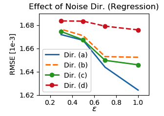
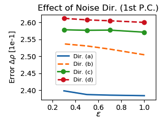
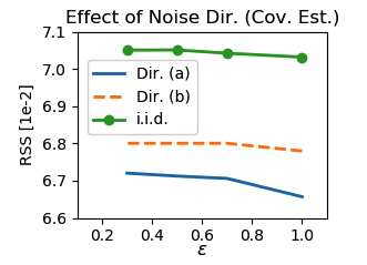
Figure 4. Effect of noise directions on the utility (all with $\delta=1/N$). (Left) Exp. I: regression on the Liver dataset. The four directions shown put more precision budget on the following features: (a) {ALT, Y}, (b) {ALT}, (c) {Y}, (d) {ALT, AST, Y}. (Middle) Exp. II: $1^{st}$ P.C. on the Movement dataset. The four directions emphasize the following features: (a) {ANC0, ANC3}, (b) {ANC0}, (c) {ANC3}, (d) {ANC1, ANC2}. (Right) Exp. III: covariance estimation on the CTG dataset. The two directions emphasize the two disjoint subsets of features: (a) {FHR, ASV, ALV}, (b) The rest of the features.

Table 5 reports the results for Exp. III. Here are the key observations.

• Compared to the non-private baseline, the MVG mechanism has very small RSS error of $.06657$.

• Compared to other $(\epsilon,\delta)$-basic mechanisms, i.e. the Gaussian mechanism and the JL transform, the MVG mechanism provides better utility with the same privacy guarantee (.004 and .001 smaller RSS error, respectively).

• Compared to other $\epsilon$-basic mechanisms, i.e. the Laplace and Exponential mechanisms, the MVG mechanism gives better utility with slightly weaker $(\epsilon,1/N)$-differential privacy guarantee (.005 and .006 smaller RSS error, respectively).

Overall, the MVG mechanism provides the best utility (smallest error). When compared to other methods with stronger privacy guarantee, the MVG mechanism can provide much higher utility. Again, we point out that in some settings, the trade-off of weaker privacy for better utility might be favorable (Fienberg et al., 2010; Duchi et al., 2013), and our approach provides the best trade-off.

9. Discussion and Future Works

9.1. Effect of Directional Noise on Utility

In Sec. 5.4, we discuss how the choice of noise directions can affect the utility. Here, we investigate this effect on the obtained utility in the three experiments. Fig. 4 depicts our results.

Fig. 4, Left, shows the direction comparison from Exp. I. We compare four choices of directions. Direction (a), which uses the domain knowledge (ALT) and the teacher label (Y), yields the best result when compared to: (b) using only the domain knowledge (ALT), (c) using only the teacher label (Y), and (d) using an arbitrary extra feature (ALT+Y+AST).

Fig. 4, Middle, shows the direction comparison from Exp. II. We compare four choices of directions. Direction (a), which makes full use of the prior information (ANC0 and ANC3), performs best when compared to: (b), (c) using only partial prior information (ANC0 or ANC3, respectively), and (d) having the wrong priors completely (ANC1 and ANC2).

Fig. 4, Right, shows the comparison from Exp. III. We compare three choices of directions. Direction (a), which uses the domain knowledge (FHR, ASV, ALV3), gives the best performance compared to: (b) using the completely wrong priors (all other features), and (c) having no prior at all (i.i.d.).

The results illustrate three key points. First, as seen in all three plots in Fig. 4, the choice of directions has an effect on the performance. Second, as indicated by Fig. 4, Right, directional noise performs much better than i.i.d. noise. Third, as seen in Fig. 4, Left and Middle, there may be multiple instances of directional noise that can lead to comparable performance. The last observation shows the promise of the notion of directional noise, as it signals the robustness of the approach.

9.2. Runtime Comparison

Method	Runtime (ms)
	Exp. I	Exp. II	Exp. III
MVG	36.2	1.8	$3.2\times 10^{3}$
Gaussian ((Dwork et al., 2006a), (Dwork et al., 2014))	1.0	0.4	10.0
JL transform ((Upadhyay, 2014a), (Blocki et al., 2012))	192.7	637.4	$2.57\times 10^{6}$
Laplace ((Dwork et al., 2006b))	0.4	0.5	8.0
Exponential ((Blum et al., 2013), (Chaudhuri et al., 2012))	627.2	2,112.7	$2.00\times 10^{6}$

Table 6. Runtime of each method on the three experiments.

Next, we present the empirical runtime comparison between the MVG mechanism and the compared methods in Table 6. The experiments are run on an AMD Opteron 6320 Processor with 4 cores using Python 2.7, along with NumPy (Oliphant, 2006), SciPy (Jones et al., 01), Scikit-learn (Pedregosa et al., 2011), and emcee (Foreman-Mackey et al., 2013) packages. The results show that, although the MVG mechanism runs much slower than the Gaussian and Laplace mechanisms, it runs much faster than the JL transform and the Exponential mechanism.

Both observations are as expected. First, the MVG mechanism runs slower than the i.i.d.-based Gaussian and Laplace mechanisms because it incurs the computational overhead of deriving the non-i.i.d. noise. The amount of overhead depends on the size of the query output as discussed in Sec. 6.3. Second, the MVG mechanism runs much faster than the JL transform because, in addition to requiring SVD to modify the singular values of the matrix query and i.i.d. Gaussian samples similar to the MVG mechanism, the JL transform has a runtime overhead for the construction of its projection matrix, which consists of multiple matrix multiplications. Finally, the MVG mechanism runs much faster than the Exponential mechanism since drawing samples from the distribution defined by the Exponential mechanism may not be efficient.

9.3. Directional Noise as a Generalized Subspace Projection

Directional noise provides utility gain by adding less noise in useful directions and more in the others. This has a connection to subspace projection or dimensionality reduction, which simply removes the non-useful directions. The main difference between the two is that, in directional noise, the non-useful directions are kept, although are highly perturbed. However, despite being highly perturbed, these directions may still be able to contribute to the utility performance.

We test this hypothesis by running two additional regression experiments (Exp. I) as follows. Given the same two important features (ALT & Y), we use the Gaussian mechanism (Dwork et al., 2006a) and the JL transform method (Upadhyay, 2014a) to perform the regression task using only these two features. With $\epsilon=1$ and $\delta=1/N$, the results are $(2.538\pm.065)\times 10^{-2}$ and $(2.863\pm.022)\times 10^{-2}$ of RMSE, respectively. Noticeably, these results are significantly worse than that of the MVG mechanism, with the same privacy guarantee. Specifically, by incorporating all features with directional noise via the MVG mechanism, we can achieve over 150% gain in utility over the dimensionality reduction alternatives.

9.4. Exploiting Structural Characteristics of the Matrices

In this work, we derive the sufficient condition for the MVG mechanism without making any assumption on the query function. However, many practical matrix-valued query functions have a specific structure, e.g. the covariance matrix is positive semi definite (PSD) (Horn and Johnson, 2012), the Laplacian matrix (Godsil and Royle, 2013) is symmetric. Therefore, future works may look into exploiting these intrinsic characteristics of the matrices in the derivation of the differential-privacy condition for the MVG mechanism.

9.5. Precision Allocation Strategy Design

Alg. 1 and Alg. 2 take as an input the precision allocation strategy vector $\boldsymbol{\theta}\in(0,1)^{m}$:$\bigl{|}\boldsymbol{\theta}\bigr{|}_{1}=1$. Elements of $\boldsymbol{\theta}$ are chosen to emphasize how informative or useful each direction is. The design of $\boldsymbol{\theta}$ to optimize the utility gain via the directional noise is an interesting topic for future research. For example, in our experiments, we use the intuition that our prior knowledge only tells us whether the directions are highly informative or not, but we do not know the granularity of the level of usefulness of these directions. Hence, we adopt the binary allocation strategy, i.e. give most precision budget to the useful directions in equal amount, and give the rest of the budget to the other directions in equal amount. An interesting direction for future work is to investigate general instances when the knowledge about the directions is more granular.

10. Conclusion

We study the matrix-valued query function in differential privacy, and present the MVG mechanism that is designed specifically for this type of query function. We prove that the MVG mechanism guarantees ($\epsilon,\delta$)-differential privacy, and, consequently, introduce the novel concept of directional noise, which can be used to reduce the impact of the noise on the utility of the query answer. Finally, we evaluate our approach experimentally for three matrix-valued query functions on three privacy-sensitive datasets, and the results show that our approach can provide the utility improvement over existing methods in all of the experiments.

Appendix A Full Proof of $(\epsilon,\delta)$-Differential Privacy

We present the full proof of the sufficient condition for the MVG mechanism to guarantee $(\epsilon,\delta)$-differential privacy presented in Theorem 3 here.

Proof.

The MVG mechanism guarantees differential privacy if for every pair of neighboring datasets $\{\mathbf{X}_{1},\mathbf{X}_{2}\}$ and all possible measurable sets $\mathbf{S}\subseteq\mathbb{R}^{m\times n}$,

$$\Pr\left[f(\mathbf{X}_{1})+\mathcal{Z}\in\mathbf{S}\right]\leq\exp(\epsilon)\Pr\left[f(\mathbf{X}_{2})+\mathcal{Z}\in\mathbf{S}\right].$$

The proof now follows by observing that (Lemma 4),

$$\mathcal{Z}=\mathbf{W}_{\boldsymbol{\Sigma}}\boldsymbol{\Lambda}_{\boldsymbol{\Sigma}}^{1/2}\mathcal{N}\boldsymbol{\Lambda}_{\boldsymbol{\Psi}}^{1/2}\mathbf{W}_{\boldsymbol{\Psi}}^{T},$$

and defining the following events:

$$\mathbf{R}_{1}=\{\mathcal{N}:\|\mathcal{N}\|_{F}^{2}\leq\zeta(\delta)^{2}\},\,\mathbf{R}_{2}=\{\mathcal{N}:\|\mathcal{N}\|_{F}^{2}>\zeta(\delta)^{2}\},$$

where $\zeta(\delta)$ is defined in Theorem 2. Next, observe that

$$\Pr\left[f(\mathbf{X}_{1})+\mathcal{Z}\in\mathbf{S}\right]$$

$$=\Pr\left[\left(\{f(\mathbf{X}_{1})+\mathcal{Z}\in\mathbf{S}\}\cap\mathbf{R}_{1}\right)\cup\left(\{f(\mathbf{X}_{1})+\mathcal{Z}\in\mathbf{S}\}\cap\mathbf{R}_{2}\right)\right]$$

$$\leq\Pr\left[\{f(\mathbf{X}_{1})+\mathcal{Z}\in\mathbf{S}\}\cap\mathbf{R}_{1}\right]+\Pr\left[\{f(\mathbf{X}_{1})+\mathcal{Z}\in\mathbf{S}\}\cap\mathbf{R}_{2}\right],$$

where the last inequality follows from the union bound. By Theorem 2 and the definition of the set $\mathbf{R}_{2}$, we have,

$$\Pr\left[\{f(\mathbf{X}_{1})+\mathcal{Z}\in\mathbf{S}\}\cap\mathbf{R}_{2}\right]\leq\Pr\left[\mathbf{R}_{2}\right]=1-\Pr\left[\mathbf{R}_{1}\right]\leq\delta.$$

In the rest of the proof, we find sufficient conditions for the following inequality to hold:

$$\Pr\left[f(\mathbf{X}_{1})+\mathcal{Z}\in(\mathbf{S}\cap\mathbf{R}_{1})\right]\leq\exp(\epsilon)\Pr\left[f(\mathbf{X}_{2})+\mathcal{Z}\in\mathbf{S}\right].$$

this would complete the proof of differential privacy guarantee.

Using the definition of $\mathcal{MVG}_{m,n}(\mathbf{0},\boldsymbol{\Sigma},\boldsymbol{\Psi})$ (Definition 2), this is satisfied if we have,

$$\int_{\mathbf{S}\cap\mathbf{R}_{1}}e^{\{-\frac{1}{2}\mathrm{tr}[\boldsymbol{\Psi}^{-1}(\mathbf{Y}-f(\mathbf{X}_{1}))^{T}\boldsymbol{\Sigma}^{-1}(\mathbf{Y}-f(\mathbf{X}_{1}))]\}}d\mathbf{Y} \leq$$

$$e^{\epsilon}\int_{\mathbf{S}\cap\mathbf{R}_{1}}e^{\{-\frac{1}{2}\mathrm{tr}[\boldsymbol{\Psi}^{-1}(\mathbf{Y}-f(\mathbf{X}_{2}))^{T}\boldsymbol{\Sigma}^{-1}(\mathbf{Y}-f(\mathbf{X}_{2}))]\}}d\mathbf{Y}.$$

By inserting $\frac{\exp\{-\frac{1}{2}\mathrm{tr}[\boldsymbol{\Psi}^{-1}(\mathbf{Y}-f(\mathbf{X}_{2}))^{T}\boldsymbol{\Sigma}^{-1}(\mathbf{Y}-f(\mathbf{X}_{2}))]\}}{\exp\{-\frac{1}{2}\mathrm{tr}[\boldsymbol{\Psi}^{-1}(\mathbf{Y}-f(\mathbf{X}_{2}))^{T}\boldsymbol{\Sigma}^{-1}(\mathbf{Y}-f(\mathbf{X}_{2}))]\}}$ inside the integral on the left side, it is sufficient to show that

$$\frac{\exp\{-\frac{1}{2}\mathrm{tr}[\boldsymbol{\Psi}^{-1}(\mathbf{Y}-f(\mathbf{X}_{1}))^{T}\boldsymbol{\Sigma}^{-1}(\mathbf{Y}-f(\mathbf{X}_{1}))]\}}{\exp\{-\frac{1}{2}\mathrm{tr}[\boldsymbol{\Psi}^{-1}(\mathbf{Y}-f(\mathbf{X}_{2}))^{T}\boldsymbol{\Sigma}^{-1}(\mathbf{Y}-f(\mathbf{X}_{2}))]\}}\leq\exp(\epsilon),$$

for all $\mathbf{Y}\in\mathbf{S}\cap\mathbf{R}_{1}$. With some algebraic manipulations, the left hand side of this condition can be expressed as,

$$= \exp\{-\frac{1}{2}\mathrm{tr}[\boldsymbol{\Psi}^{-1}\mathbf{Y}{}^{T}\mathbf{\boldsymbol{\Sigma}}^{-1}(f(\mathbf{X}_{2})-f(\mathbf{X}_{1}))$$

$$+\boldsymbol{\Psi}^{-1}(f(\mathbf{X}_{2})-f(\mathbf{X}_{1}))^{T}\boldsymbol{\Sigma}^{-1}\mathbf{Y}]\}$$

$$-\boldsymbol{\Psi}^{-1}f(\mathbf{X}_{2})^{T}\boldsymbol{\Sigma}^{-1}f(\mathbf{X}_{2})+\boldsymbol{\Psi}^{-1}f(\mathbf{X}_{1})^{T}\boldsymbol{\Sigma}^{-1}f(\mathbf{X}_{1})$$

$$= \exp\{\frac{1}{2}\mathrm{tr}[\boldsymbol{\Psi}^{-1}\mathbf{Y}^{T}\mathbf{\boldsymbol{\Sigma}}^{-1}\boldsymbol{\Delta}+\boldsymbol{\Psi}^{-1}\boldsymbol{\Delta}^{T}\boldsymbol{\Sigma}^{-1}\mathbf{Y}$$

$$+\boldsymbol{\Psi}^{-1}f(\mathbf{X}_{2})^{T}\boldsymbol{\Sigma}^{-1}f(\mathbf{X}_{2})-\boldsymbol{\Psi}^{-1}f(\mathbf{X}_{1})^{T}\boldsymbol{\Sigma}^{-1}f(\mathbf{X}_{1})]\},$$

where $\boldsymbol{\Delta}=f(\mathbf{X}_{1})-f(\mathbf{X}_{2})$. This quantity has to be bounded by $\leq\exp(\epsilon)$, so we present the following characteristic equation, which has to be satisfied for all possible neighboring $\{\mathbf{X}_{1},\mathbf{X}_{2}\}$ and all $\mathbf{Y}\in\mathbf{S}\cap\mathbf{R}_{1}$, for the MVG mechanism to guarantee $(\epsilon,\delta)$-differential privacy:

$$\mathrm{tr}[\boldsymbol{\Psi}^{-1}\mathcal{Y}^{T}\boldsymbol{\Sigma}^{-1}\boldsymbol{\Delta}+\boldsymbol{\Psi}^{-1}\boldsymbol{\Delta}^{T}\boldsymbol{\Sigma}^{-1}\mathcal{Y}$$

$$+\boldsymbol{\Psi}^{-1}f(\mathbf{X}_{2})^{T}\boldsymbol{\Sigma}^{-1}f(\mathbf{X}_{2})-\boldsymbol{\Psi}^{-1}f(\mathbf{X}_{1})^{T}\boldsymbol{\Sigma}^{-1}f(\mathbf{X}_{1})] \leq 2\epsilon.$$

Specifically, we want to show that this inequality holds with probability $1-\delta$.

From the characteristic equation, the proof analyzes the four terms in the sum separately since the trace is additive.

The first term: $\mathrm{tr}[\boldsymbol{\Psi}^{-1}\mathbf{Y}^{T}\boldsymbol{\Sigma}^{-1}\boldsymbol{\Delta}]$. First, let us denote $\mathcal{Y}=f(\mathbf{X})+\mathcal{Z}$, where $f(\mathbf{X})$ and $\mathcal{Z}$ are any possible instances of the query and the noise, respectively. Then, we can rewrite the first term as, $\mathrm{tr}[\boldsymbol{\Psi}^{-1}f(\mathbf{X})^{T}\boldsymbol{\Sigma}^{-1}\boldsymbol{\Delta}]+\mathrm{tr}[\boldsymbol{\Psi}^{-1}\mathcal{Z}^{T}\boldsymbol{\Sigma}^{-1}\boldsymbol{\Delta}]$. The earlier part can be bounded from Lemma 2:

$$\mathrm{tr}[\boldsymbol{\Psi}^{-1}f(\mathbf{X})^{T}\boldsymbol{\Sigma}^{-1}\boldsymbol{\Delta}]\leq\sum_{i=1}^{r}\sigma_{i}(\boldsymbol{\Psi}^{-1}f(\mathbf{X})^{T})\sigma_{i}(\boldsymbol{\Delta}^{T}\boldsymbol{\Sigma}^{-1}).$$

Lemma 1 can then be used to bound each singular value. In more detail,

$$\sigma_{i}(\boldsymbol{\Psi}^{-1}f(\mathbf{X})^{T})\leq\frac{\left\|\boldsymbol{\Psi}^{-1}f(\mathbf{X})^{T}\right\|_{F}}{\sqrt{i}}\leq\frac{\left\|\boldsymbol{\Psi}^{-1}\right\|_{F}\left\|f(\mathbf{X})\right\|_{F}}{\sqrt{i}},$$

where the last inequality is via the sub-multiplicative property of a matrix norm (Meyer, 2000). It is well-known that $\bigl{\|}\boldsymbol{\Psi}^{-1}\bigr{\|}_{F}=\bigl{\|}\boldsymbol{\sigma}(\boldsymbol{\Psi}^{-1})\bigr{\|}_{2}$ (cf. (Horn and Johnson, 2012, p. 342)), and since $\gamma=\sup_{\mathbf{X}}\bigl{\|}f(\mathbf{X})\bigr{\|}_{F}$,

$$\sigma_{i}(\boldsymbol{\Psi}^{-1}f(\mathbf{X})^{T})\leq\gamma\left\|\boldsymbol{\sigma}(\boldsymbol{\Psi}^{-1})\right\|_{2}/\sqrt{i}.$$

Applying the same steps to the other singular value, and using Definition 3, we can write,

$$\sigma_{i}(\boldsymbol{\Delta}^{T}\boldsymbol{\Sigma}^{-1})\leq s_{2}(f)\left\|\boldsymbol{\sigma}(\boldsymbol{\Sigma}^{-1})\right\|_{2}/\sqrt{i}.$$

By substituting the two singular value bounds, the earlier part of the first term can be bounded by,

$$\mathrm{tr}[\boldsymbol{\Psi}^{-1}f(\mathbf{X})^{T}\boldsymbol{\Sigma}^{-1}\boldsymbol{\Delta}]$$

(6) $$\leq \gamma s_{2}(f)H_{r}\left\|\boldsymbol{\sigma}(\boldsymbol{\Sigma}^{-1})\right\|_{2}\left\|\boldsymbol{\sigma}(\boldsymbol{\Psi}^{-1})\right\|_{2}.$$

The latter part of the first term is more complicated since it involves $\mathcal{Z}$, so we will derive the bound in more detail. First, let us define $\mathcal{N}$ to be drawn from $\mathcal{MVG}_{m,n}(\mathbf{0},\mathbf{I}_{m},\mathbf{I}_{n})$, so we can write $\mathcal{Z}$ in terms of $\mathcal{N}$ using affine transformation (Dawid, 1981): $\mathcal{Z}=\mathbf{B}_{\boldsymbol{\Sigma}}\mathcal{N}\mathbf{B}_{\boldsymbol{\Psi}}^{T}$. To specify $\mathbf{B}_{\boldsymbol{\Sigma}}$ and $\mathbf{B}_{\boldsymbol{\Psi}}$, we solve the following linear equations, respectively,

$$\mathbf{B}_{\boldsymbol{\Sigma}}\mathbf{B}_{\boldsymbol{\Sigma}}^{T}=\boldsymbol{\Sigma};\mathbf{B}_{\boldsymbol{\Psi}}\mathbf{B}_{\boldsymbol{\Psi}}^{T}=\boldsymbol{\Psi}.$$

This can be readily solved with SVD (cf. (Horn and Johnson, 2012, p. 440)); hence, $\mathbf{B}_{\boldsymbol{\Sigma}}=\mathbf{W}_{\boldsymbol{\Sigma}}\boldsymbol{\Lambda}_{\boldsymbol{\Sigma}}^{\frac{1}{2}}$, and $\mathbf{B}_{\boldsymbol{\Psi}}=\mathbf{W}_{\boldsymbol{\Psi}}\boldsymbol{\Lambda}_{\boldsymbol{\Psi}}^{\frac{1}{2}}$, where $\boldsymbol{\Sigma}=\mathbf{W}_{\boldsymbol{\Sigma}}\boldsymbol{\Lambda}_{\boldsymbol{\Sigma}}\mathbf{W}_{\boldsymbol{\Sigma}}^{T}$, and $\boldsymbol{\Psi}=\mathbf{W}_{\boldsymbol{\Psi}}\boldsymbol{\Lambda}_{\boldsymbol{\Psi}}\mathbf{W}_{\boldsymbol{\Psi}}^{T}$ from SVD. Therefore, $\mathcal{Z}$ can be written as,

$$\mathcal{Z}=\mathbf{W}_{\boldsymbol{\Sigma}}\boldsymbol{\Lambda}_{\boldsymbol{\Sigma}}^{1/2}\mathcal{N}\boldsymbol{\Lambda}_{\boldsymbol{\Psi}}^{1/2}\mathbf{W}_{\boldsymbol{\Psi}}^{T}.$$

Substituting into the latter part of the first term yields,

$$\mathrm{tr}[\boldsymbol{\Psi}^{-1}\mathcal{Z}^{T}\boldsymbol{\Sigma}^{-1}\boldsymbol{\Delta}]=\mathrm{tr}[\mathbf{W}_{\boldsymbol{\Psi}}\boldsymbol{\Lambda}_{\boldsymbol{\Psi}}^{-1/2}\mathcal{N}\boldsymbol{\Lambda}_{\boldsymbol{\Sigma}}^{-1/2}\mathbf{W}_{\boldsymbol{\Sigma}}^{T}\boldsymbol{\Delta}].$$

This can be bounded by Lemma 2 as,

$$\mathrm{tr}[\boldsymbol{\Psi}^{-1}\mathcal{Z}^{T}\boldsymbol{\Sigma}^{-1}\boldsymbol{\Delta}]\leq\sum_{i=1}^{r}\sigma_{i}(\mathbf{W}_{\boldsymbol{\Psi}}\boldsymbol{\Lambda}_{\boldsymbol{\Psi}}^{-1/2}\mathcal{N}\boldsymbol{\Lambda}_{\boldsymbol{\Sigma}}^{-1/2}\mathbf{W}_{\boldsymbol{\Sigma}}^{T})\sigma_{i}(\boldsymbol{\Delta}).$$

The two singular values can then be bounded by Lemma 1. For the first singular value,

$$\sigma_{i}(\mathbf{W}_{\boldsymbol{\Psi}}\boldsymbol{\Lambda}_{\boldsymbol{\Psi}}^{-1/2}\mathcal{N}\boldsymbol{\Lambda}_{\boldsymbol{\Sigma}}^{-1/2}\mathbf{W}_{\boldsymbol{\Sigma}}^{T}) \leq\frac{\left\|\mathbf{W}_{\boldsymbol{\Psi}}\boldsymbol{\Lambda}_{\boldsymbol{\Psi}}^{-1/2}\mathcal{N}\boldsymbol{\Lambda}_{\boldsymbol{\Sigma}}^{-1/2}\mathbf{W}_{\boldsymbol{\Sigma}}^{T}\right\|_{F}}{\sqrt{i}}$$

$$\leq\frac{\left\|\boldsymbol{\Lambda}_{\boldsymbol{\Sigma}}^{-1/2}\right\|_{F}\left\|\boldsymbol{\Lambda}_{\boldsymbol{\Psi}}^{-1/2}\right\|_{F}\left\|\mathcal{N}\right\|_{F}}{\sqrt{i}}.$$

By definition, $\left\|\boldsymbol{\Lambda}_{\boldsymbol{\Sigma}}^{-1/2}\right\|_{F}=\sqrt{\mathrm{tr}(\boldsymbol{\Lambda}_{\boldsymbol{\Sigma}}^{-1})}=\left\|\boldsymbol{\sigma}(\boldsymbol{\Sigma}^{-1})\right\|_{1}^{1/2}$, where $\left\|\cdot\right\|_{1}$ is the 1-norm. By norm relation, $\left\|\boldsymbol{\sigma}(\boldsymbol{\Sigma}^{-1})\right\|_{1}^{1/2}\leq m^{1/4}\left\|\boldsymbol{\sigma}(\boldsymbol{\Sigma}^{-1})\right\|_{2}^{1/2}$. With similar derivation for $\bigl{\|}\boldsymbol{\Lambda}_{\boldsymbol{\Psi}}^{-1/2}\bigr{\|}_{F}$ and with Theorem 2, the singular value can be bounded with probability $1-\delta$ as,

$$\sigma_{i}(\mathbf{W}_{\boldsymbol{\Psi}}\boldsymbol{\Lambda}_{\boldsymbol{\Psi}}^{-\frac{1}{2}}\mathcal{N}\boldsymbol{\Lambda}_{\boldsymbol{\Sigma}}^{-\frac{1}{2}}\mathbf{W}_{\boldsymbol{\Sigma}}^{T})$$

$$\leq \frac{(mn)^{\frac{1}{4}}\zeta(\delta)\left\|\boldsymbol{\sigma}(\boldsymbol{\Sigma}^{-1})\right\|_{2}^{\frac{1}{2}}\left\|\boldsymbol{\sigma}(\boldsymbol{\Psi}^{-1})\right\|_{2}^{\frac{1}{2}}}{\sqrt{i}}.$$

Meanwhile, the other singular value can be readily bounded with Lemma 1 as $\sigma_{i}(\boldsymbol{\Delta})\leq s_{2}(f)/\sqrt{i}$. Hence, the latter part of the first term is bounded with probability $\geq 1-\delta$ as,

$$\mathrm{tr}[\boldsymbol{\Psi}^{-1}\mathbf{Z}^{T}\boldsymbol{\Sigma}^{-1}\boldsymbol{\Delta}]$$

(7) $$\leq (mn)^{\frac{1}{4}}\zeta(\delta)H_{r}s_{2}(f)\left\|\boldsymbol{\sigma}(\boldsymbol{\Sigma}^{-1})\right\|_{2}^{\frac{1}{2}}\left\|\boldsymbol{\sigma}(\boldsymbol{\Psi}^{-1})\right\|_{2}^{\frac{1}{2}}.$$

Since the parameter $(\left\|\boldsymbol{\sigma}(\boldsymbol{\Sigma}^{-1})\right\|_{2}\left\|\boldsymbol{\sigma}(\boldsymbol{\Psi}^{-1})\right\|_{2})^{1/2}$ appears a lot in the derivation, let us define

$$\phi=(\left\|\boldsymbol{\sigma}(\boldsymbol{\Sigma}^{-1})\right\|_{2}\left\|\boldsymbol{\sigma}(\boldsymbol{\Psi}^{-1})\right\|_{2})^{1/2}.$$

Finally, combining Eq. (6) and (7) yields the bound for the first term,

$$\mathrm{tr}[\boldsymbol{\Psi}^{-1}\mathbf{Y}^{T}\boldsymbol{\Sigma}^{-1}\boldsymbol{\Delta}]\leq\gamma H_{r}s_{2}(f)\phi^{2}+(mn)^{1/4}\zeta(\delta)H_{r}s_{2}(f)\phi.$$

The second term: $\mathrm{tr}[\boldsymbol{\Psi}^{-1}\boldsymbol{\Delta}^{T}\boldsymbol{\Sigma}^{-1}\mathbf{Y}]$. By following the same steps as in the first term, it can be shown that the second term has the exact same bound as the first terms, i.e.

$$\mathrm{tr}[\boldsymbol{\Psi}^{-1}\boldsymbol{\Delta}^{T}\boldsymbol{\Sigma}^{-1}\mathbf{Y}]\leq\gamma H_{r}s_{2}(f)\phi^{2}+(mn)^{1/4}\zeta(\delta)H_{r}s_{2}(f)\phi.$$

The third term: $\mathrm{tr}[\boldsymbol{\Psi}^{-1}f(\mathbf{X}_{2})^{T}\boldsymbol{\Sigma}^{-1}f(\mathbf{X}_{2})]$. Applying Lemma 2 and 1, we can readily bound it as,

$$\mathrm{tr}[\boldsymbol{\Psi}^{-1}f(\mathbf{X}_{2})^{T}\boldsymbol{\Sigma}^{-1}f(\mathbf{X}_{2})]\leq\gamma^{2}H_{r}\phi^{2}.$$

The fourth term: $-\mathrm{tr}[\boldsymbol{\Psi}^{-1}f(\mathbf{X}_{1})^{T}\boldsymbol{\Sigma}^{-1}f(\mathbf{X}_{1})]$. Since this term has the negative sign, we consider the absolute value instead. Using Lemma 3,

$$\left|\mathrm{tr}[\boldsymbol{\Psi}^{-1}f(\mathbf{X}_{1})^{T}\boldsymbol{\Sigma}^{-1}f(\mathbf{X}_{1})]\right|\leq\sum_{i=1}^{r}\sigma_{i}(\boldsymbol{\Psi}^{-1}f(\mathbf{X}_{1})^{T}\boldsymbol{\Sigma}^{-1}f(\mathbf{X}_{1})).$$

Then, using the singular value bound in Lemma 1,

$$\sigma_{i}(\boldsymbol{\Psi}^{-1}f(\mathbf{X}_{1})^{T}\boldsymbol{\Sigma}^{-1}f(\mathbf{X}_{1}))\leq\frac{\left\|\boldsymbol{\Psi}^{-1}\right\|_{F}\left\|f(\mathbf{X}_{1})\right\|_{F}^{2}\left\|\boldsymbol{\Sigma}^{-1}\right\|_{F}}{\sqrt{i}}.$$

Hence, the fourth term can be bounded by,

$$\left|\mathrm{tr}[\boldsymbol{\Psi}^{-1}f(\mathbf{X}_{1})^{T}\boldsymbol{\Sigma}^{-1}f(\mathbf{X}_{1})]\right|\leq\gamma^{2}H_{r,1/2}\phi^{2}.$$

Four terms combined: by combining the four terms and rearranging them, the characteristic equation becomes,

$$\alpha\phi^{2}+\beta\phi\leq 2\epsilon.$$

This is a quadratic equation, of which the solution is known to be $\phi\in[\frac{-\beta-\sqrt{\beta^{2}+8\alpha\epsilon}}{2\alpha},\frac{-\beta+\sqrt{\beta^{2}+8\alpha\epsilon}}{2\alpha}]$. Since we know $\phi>0$, we only have the one-sided solution,

$$\phi\leq\frac{-\beta+\sqrt{\beta^{2}+8\alpha\epsilon}}{2\alpha},$$

which implies the criterion in Theorem 3. ∎

Appendix B $L_{2}$-Sensitivities

Here, we derive the $L_{2}$-sensitivity for the MVG mechanism used in our experiments.

B.1. Experiment I

The query function is $f(\mathbf{X})=\mathbf{X}\in[0,1]^{6\times 248}$. For neighboring datasets $\{\mathbf{X},\mathbf{X}^{\prime}\}$, the $L_{2}$-sensitivity is

$$s_{2}(f)=\sup_{\mathbf{X},\mathbf{X}^{\prime}}\left\|\mathbf{X}-\mathbf{X}^{\prime}\right\|_{F}=\sup_{\mathbf{X},\mathbf{X}^{\prime}}\sqrt{\sum_{i=1}^{6}(x(i)-x^{\prime}(i))^{2}}=\sqrt{6}.$$

B.2. Experiment II

The query function is $f(\mathbf{X})=\frac{1}{N}\mathbf{X}\mathbf{X}^{T}$, where $\mathbf{X}\in[-1,1]^{4\times 2021}$. For neighboring datasets $\{\mathbf{X},\mathbf{X}^{\prime}\}$, the $L_{2}$-sensitivity is

$$s_{2}(f)=\sup_{\mathbf{X},\mathbf{X}^{\prime}}\frac{\left\|\mathbf{x}_{j}\mathbf{x}_{j}^{T}-\mathbf{x}_{j}^{\prime}\mathbf{x}_{j}^{\prime T}\right\|_{F}}{2021}=\frac{2\sqrt{\sum_{j=1}^{4^{2}}x_{j}(i)^{2}}}{2021}=\frac{8}{2021}.$$

B.3. Experiment III

The query function is the same as Exp. I, so the $L_{2}$-sensitivity can be readily derived as $s_{2}(f)=\sup_{\mathbf{X},\mathbf{X}^{\prime}}\sqrt{\sum_{i=1}^{21}(x(i)-x^{\prime}(i))^{2}}=\sqrt{21}$.

References

- (1)
- Abdi (2007) Herve Abdi. 2007. Singular value decomposition (SVD) and generalized singular value decomposition. Encyclopedia of Measurement and Statistics. Thousand Oaks (CA): Sage (2007), 907–912.
- Acs et al. (2012) Gergely Acs, Claude Castelluccia, and Rui Chen. 2012. Differentially private histogram publishing through lossy compression. In ICDM. IEEE.
- Alatalo et al. (2008) P. I. Alatalo, H. M. Koivisto, J. P. Hietala, K. S. Puukka, R. Bloigu, and O. J. Niemela. 2008. Effect of moderate alcohol consumption on liver enzymes increases with increasing body mass index. AJCN 88, 4 (Oct 2008), 1097–1103.
- Bacciu et al. (2014) Davide Bacciu, Paolo Barsocchi, Stefano Chessa, Claudio Gallicchio, and Alessio Micheli. 2014. An experimental characterization of reservoir computing in ambient assisted living applications. Neural Computing and Applications 24, 6 (2014), 1451–1464.
- Bell et al. (2008) Robert M. Bell, Yehuda Koren, and Chris Volinsky. 2008. The bellkor 2008 solution to the netflix prize. Statistics Research Department at AT&T Research (2008).
- Bishop (2006) Christopher M. Bishop. 2006. Pattern recognition. Machine Learning 128 (2006).
- Blocki et al. (2012) Jeremiah Blocki, Avrim Blum, Anupam Datta, and Or Sheffet. 2012. The johnson-lindenstrauss transform itself preserves differential privacy. In FOCS. IEEE.
- Blum et al. (2005) Avrim Blum, Cynthia Dwork, Frank McSherry, and Kobbi Nissim. 2005. Practical privacy: the SuLQ framework. In PODS. ACM.
- Blum et al. (2013) Avrim Blum, Katrina Ligett, and Aaron Roth. 2013. A learning theory approach to noninteractive database privacy. JACM 60, 2 (2013), 12.
- Blum and Roth (2013) Avrim Blum and Aaron Roth. 2013. Fast private data release algorithms for sparse queries. Springer, 395–410.
- Chanyaswad et al. (2018) Thee Chanyaswad, Alex Dytso, H Vincent Poor, and Prateek Mittal. 2018. A Differential Privacy Mechanism Design Under Matrix-Valued Query. arXiv preprint arXiv:1802.10077 (2018).
- Chanyaswad et al. (2017) Thee Chanyaswad, Changchang Liu, and Prateek Mittal. 2017. Coupling Random Orthonormal Projection with Gaussian Generative Model for Non-Interactive Private Data Release. arXiv:1709.00054 (2017).
- Chaudhuri et al. (2012) Kamalika Chaudhuri, Anand Sarwate, and Kaushik Sinha. 2012. Near-optimal differentially private principal components. In NIPS.
- Chaudhuri and Vinterbo (2013) Kamalika Chaudhuri and Staal A. Vinterbo. 2013. A stability-based validation procedure for differentially private machine learning. In NIPS.
- Cormode et al. (2012) Graham Cormode, Cecilia Procopiuc, Divesh Srivastava, Entong Shen, and Ting Yu. 2012. Differentially private spatial decompositions. In ICDE. IEEE.
- Dawid (1981) A. Philip Dawid. 1981. Some matrix-variate distribution theory: notational considerations and a Bayesian application. Biometrika 68, 1 (1981), 265–274.
- Day and Li (2015) Wei-Yen Day and Ninghui Li. 2015. Differentially private publishing of high-dimensional data using sensitivity control. In CCS. ACM.
- de Campos et al. (2000) Diogo Ayres de Campos, Joao Bernardes, Antonio Garrido, Joaquim Marques de Sa, and Luis Pereira-Leite. 2000. SisPorto 2.0: a program for automated analysis of cardiotocograms. Journal of Maternal-Fetal Medicine 9, 5 (2000), 311–318.
- Duchi et al. (2013) John C. Duchi, Michael I. Jordan, and Martin J. Wainwright. 2013. Local privacy and statistical minimax rates. In FOCS. IEEE.
- Dutilleul (1999) Pierre Dutilleul. 1999. The MLE algorithm for the matrix normal distribution. Journal of statistical computation and simulation 64, 2 (1999), 105–123.
- Dwork (2006) Cynthia Dwork. 2006. Differential privacy. Springer, 1–12.
- Dwork (2008) Cynthia Dwork. 2008. Differential privacy: A survey of results. In TAMC. Springer.
- Dwork et al. (2006a) Cynthia Dwork, Krishnaram Kenthapadi, Frank McSherry, Ilya Mironov, and Moni Naor. 2006a. Our data, ourselves: Privacy via distributed noise generation. In EUROCRYPT. Springer.
- Dwork et al. (2006b) Cynthia Dwork, Frank McSherry, Kobbi Nissim, and Adam Smith. 2006b. Calibrating noise to sensitivity in private data analysis. In TCC. Springer.
- Dwork and Roth (2014) Cynthia Dwork and Aaron Roth. 2014. The algorithmic foundations of differential privacy. FnT-TCS 9, 3-4 (2014), 211–407.
- Dwork et al. (2010) Cynthia Dwork, Guy N. Rothblum, and Salil Vadhan. 2010. Boosting and differential privacy. In FOCS. IEEE.
- Dwork et al. (2014) Cynthia Dwork, Kunal Talwar, Abhradeep Thakurta, and Li Zhang. 2014. Analyze gauss: optimal bounds for privacy-preserving principal component analysis. In STOC. ACM.
- Fienberg et al. (2010) Stephen E. Fienberg, Alessandro Rinaldo, and Xiaolin Yang. 2010. Differential privacy and the risk-utility tradeoff for multi-dimensional contingency tables. In PSD. Springer.
- Foreman-Mackey et al. (2013) Daniel Foreman-Mackey, David W Hogg, Dustin Lang, and Jonathan Goodman. 2013. emcee: the MCMC hammer. Publications of the Astronomical Society of the Pacific 125, 925 (2013), 306.
- Forsyth and Rada (1986) Richard Forsyth and Roy Rada. 1986. Machine learning: applications in expert systems and information retrieval. Halsted Press.
- Fredrikson et al. (2014) Matthew Fredrikson, Eric Lantz, Somesh Jha, Simon Lin, David Page, and Thomas Ristenpart. 2014. Privacy in Pharmacogenetics: An End-to-End Case Study of Personalized Warfarin Dosing.. In USENIX Security.
- Friedman et al. (2001) Jerome Friedman, Trevor Hastie, and Robert Tibshirani. 2001. The elements of statistical learning. Vol. 1. Springer series in statistics New York.
- Gilks et al. (1995) Walter R. Gilks, Sylvia Richardson, and David Spiegelhalter. 1995. Markov chain Monte Carlo in practice. CRC press.
- Godsil and Royle (2013) Chris Godsil and Gordon F. Royle. 2013. Algebraic graph theory. Vol. 207. Springer Science & Business Media.
- Golub and Loan (1996) Gene H. Golub and Charles F. Van Loan. 1996. Matrix computations. Johns Hopkins University, Press, Baltimore, MD, USA (1996), 374–426.
- Gupta and Varga (1992) AK Gupta and T. Varga. 1992. Characterization of matrix variate normal distributions. Journal of Multivariate Analysis 41, 1 (1992), 80–88.
- Hardt et al. (2012) Moritz Hardt, Katrina Ligett, and Frank McSherry. 2012. A simple and practical algorithm for differentially private data release. In NIPS.
- Hardt and Roth (2012) Moritz Hardt and Aaron Roth. 2012. Beating randomized response on incoherent matrices. In Proceedings of the forty-fourth annual ACM symposium on Theory of computing. ACM, 1255–1268.
- Hardt and Roth (2013a) Moritz Hardt and Aaron Roth. 2013a. Beyond worst-case analysis in private singular vector computation. In STOC. ACM.
- Hardt and Roth (2013b) Moritz Hardt and Aaron Roth. 2013b. Beyond worst-case analysis in private singular vector computation. In Proceedings of the forty-fifth annual ACM symposium on Theory of computing. ACM, 331–340.
- Hardt and Rothblum (2010) Moritz Hardt and Guy N. Rothblum. 2010. A multiplicative weights mechanism for privacy-preserving data analysis. In FOCS. IEEE.
- Hardt and Talwar (2010) Moritz Hardt and Kunal Talwar. 2010. On the geometry of differential privacy. In Proceedings of the forty-second ACM symposium on Theory of computing. ACM, 705–714.
- Hay et al. (2016) Michael Hay, Ashwin Machanavajjhala, Gerome Miklau, Yan Chen, and Dan Zhang. 2016. Principled evaluation of differentially private algorithms using DPBench. In SIGMOD/PODS. ACM.
- Hay et al. (2010) Michael Hay, Vibhor Rastogi, Gerome Miklau, and Dan Suciu. 2010. Boosting the accuracy of differentially private histograms through consistency. PVLDB 3, 1-2 (2010), 1021–1032.
- Horn and Johnson (1991) Roger A. Horn and Charles R. Johnson. 1991. Topics in matrix analysis, 1991. Cambridge University Press 37 (1991), 39.
- Horn and Johnson (2012) Roger A. Horn and Charles R. Johnson. 2012. Matrix analysis. Cambridge university press.
- Hughes et al. (2014) John F. Hughes, Andries Van Dam, James D. Foley, and Steven K. Feiner. 2014. Computer graphics: principles and practice. Pearson Education.
- Iranmanesh et al. (2010) Anis Iranmanesh, M. Arashi, and SMM Tabatabaey. 2010. On conditional applications of matrix variate normal distribution. Iranian Journal of Mathematical Sciences and Informatics 5, 2 (2010), 33–43.
- Jiang et al. (2013) X. Jiang, Z. Ji, S. Wang, N. Mohammed, S. Cheng, and L. Ohno-Machado. 2013. Differential-Private Data Publishing Through Component Analysis. Trans. on Data Privacy 6, 1 (Apr 2013), 19–34.
- Johnson et al. (2017) Noah Johnson, Joseph P. Near, and Dawn Song. 2017. Practical Differential Privacy for SQL Queries Using Elastic Sensitivity. arXiv:1706.09479 (2017).
- Jolliffe (1986) Ian T. Jolliffe. 1986. Principal Component Analysis and Factor Analysis. Springer, 115–128.
- Jones et al. (01 ) Eric Jones, Travis Oliphant, Pearu Peterson, et al. 2001–. SciPy: Open source scientific tools for Python. http://www.scipy.org/
- Kapralov and Talwar (2013) Michael Kapralov and Kunal Talwar. 2013. On differentially private low rank approximation. In SODA. SIAM.
- Kenthapadi et al. (2012) Krishnaram Kenthapadi, Aleksandra Korolova, Ilya Mironov, and Nina Mishra. 2012. Privacy via the johnson-lindenstrauss transform. arXiv:1204.2606 (2012).
- Kung (2014) S. Y. Kung. 2014. Kernel Methods and Machine Learning. Cambridge University Press.
- Laurent and Massart (2000) Beatrice Laurent and Pascal Massart. 2000. Adaptive estimation of a quadratic functional by model selection. Annals of Statistics (2000), 1302–1338.
- Li et al. (2014) Chao Li, Michael Hay, Gerome Miklau, and Yue Wang. 2014. A data-and workload-aware algorithm for range queries under differential privacy. PVLDB 7, 5 (2014), 341–352.
- Li et al. (2010) Chao Li, Michael Hay, Vibhor Rastogi, Gerome Miklau, and Andrew McGregor. 2010. Optimizing linear counting queries under differential privacy. In PODS. ACM.
- Li and Miklau (2012) Chao Li and Gerome Miklau. 2012. An adaptive mechanism for accurate query answering under differential privacy. PVLDB 5, 6 (2012), 514–525.
- Li et al. (2011) Yang D. Li, Zhenjie Zhang, Marianne Winslett, and Yin Yang. 2011. Compressive mechanism: Utilizing sparse representation in differential privacy. In WPES. ACM.
- Lichman (2013) M. Lichman. 2013. UCI Machine Learning Repository. http://archive.ics.uci.edu/ml.
- Liu (2016a) Fang Liu. 2016a. Generalized gaussian mechanism for differential privacy. arXiv:1602.06028 (2016).
- Liu (2016b) Fang Liu. 2016b. Model-based differential private data synthesis. arXiv:1606.08052 (2016).
- Lyu et al. (2016) Min Lyu, Dong Su, and Ninghui Li. 2016. Understanding the sparse vector technique for differential privacy. arXiv:1603.01699 (2016).
- McDermott and Forsyth (2016) James McDermott and Richard S. Forsyth. 2016. Diagnosing a disorder in a classification benchmark. Pattern Recognition Letters 73 (2016), 41–43.
- McSherry and Mironov (2009) Frank McSherry and Ilya Mironov. 2009. Differentially private recommender systems: building privacy into the net. In KDD. ACM.
- McSherry and Talwar (2007) Frank McSherry and Kunal Talwar. 2007. Mechanism design via differential privacy. In FOCS. IEEE.
- Merikoski et al. (1994) Jorma Kaarlo Merikoski, Humberto Sarria, and Pablo Tarazaga. 1994. Bounds for singular values using traces. Linear Algebra Appl. 210 (1994), 227–254.
- Meyer (2000) Carl D. Meyer. 2000. Matrix analysis and applied linear algebra. Vol. 2. Siam.
- Murphy (2012) Kevin P. Murphy. 2012. Machine Learning: A Probabilistic Perspective. The MIT Press.
- Narayanan and Shmatikov (2008) Arvind Narayanan and Vitaly Shmatikov. 2008. Robust de-anonymization of large sparse datasets. In S&P. IEEE.
- Netflix (2009) Netflix. 2009. Netflix Prize. http://www.netflixprize.com/. Accessed on: 08/10/2017.
- Nguyen (1997) Truc T. Nguyen. 1997. A note on matrix variate normal distribution. Journal of Multivariate Analysis 60, 1 (1997), 148–153.
- Nikolov (2015) Aleksandar Nikolov. 2015. An improved private mechanism for small databases. In International Colloquium on Automata, Languages, and Programming. Springer, 1010–1021.
- Nikolov et al. (2013) Aleksandar Nikolov, Kunal Talwar, and Li Zhang. 2013. The geometry of differential privacy: the sparse and approximate cases. In STOC. ACM.
- Nissim et al. (2007) Kobbi Nissim, Sofya Raskhodnikova, and Adam Smith. 2007. Smooth sensitivity and sampling in private data analysis. In STOC. ACM.
- Oliphant (2006) Travis E Oliphant. 2006. A guide to NumPy. Vol. 1. Trelgol Publishing USA.
- Pedregosa et al. (2011) Fabian Pedregosa, Gaël Varoquaux, Alexandre Gramfort, Vincent Michel, Bertrand Thirion, Olivier Grisel, Mathieu Blondel, Peter Prettenhofer, Ron Weiss, and Vincent Dubourg. 2011. Scikit-learn: Machine learning in Python. JMLR 12, Oct (2011), 2825–2830.
- Proserpio et al. (2014) Davide Proserpio, Sharon Goldberg, and Frank McSherry. 2014. Calibrating data to sensitivity in private data analysis: a platform for differentially-private analysis of weighted datasets. PVLDB 7, 8 (2014), 637–648.
- Qardaji et al. (2013a) Wahbeh Qardaji, Weining Yang, and Ninghui Li. 2013a. Differentially private grids for geospatial data. In ICDE. IEEE.
- Qardaji et al. (2013b) Wahbeh Qardaji, Weining Yang, and Ninghui Li. 2013b. Understanding hierarchical methods for differentially private histograms. PVLDB 6, 14 (2013), 1954–1965.
- Rao (1964) C. Radhakrishna Rao. 1964. The use and interpretation of principal component analysis in applied research. Sankhya: The Indian Journal of Statistics, Series A (1964), 329–358.
- Santos et al. (2006) C. Costa Santos, João Bernardes, Paul MB Vitányi, and Luis Antunes. 2006. Clustering fetal heart rate tracings by compression. In CBMS. IEEE.
- Sondow and Weisstein (2017) Jonathan Sondow and Eric W. Weisstein. 2017. Harmonic Number. http://mathworld.wolfram.com/HarmonicNumber.html.
- Thacker (1989) William Carlisle Thacker. 1989. The role of the Hessian matrix in fitting models to measurements. JGR: Oceans 94, C5 (1989), 6177–6196.
- Upadhyay (2014a) Jalaj Upadhyay. 2014a. Circulant matrices and differential privacy. analysis 16 (2014), 47.
- Upadhyay (2014b) Jalaj Upadhyay. 2014b. Randomness Efficient Fast-Johnson-Lindenstrauss Transform with Applications in Differential Privacy and Compressed Sensing. arXiv:1410.2470 (2014).
- Vapnik (2013) Vladimir Vapnik. 2013. The nature of statistical learning theory. Springer science & business media.
- von Neumann (1937) J. von Neumann. 1937. Some matrix inequalities and metrization of metric space. Tomsk Univ.Rev 1 (1937), 286–296.
- Waal (2006) DJ De Waal. 2006. Matrix-Valued Distributions. Encyclopedia of statistical sciences (2006).
- White (1992) Steven R. White. 1992. Density matrix formulation for quantum renormalization groups. PRL 69, 19 (1992), 2863.
- Wikipedia (2017) Wikipedia. 2017. Matrix (mathematics). https://en.wikipedia.org/wiki/Matrix_(mathematics).
- Xiao et al. (2011a) Xiaokui Xiao, Gabriel Bender, Michael Hay, and Johannes Gehrke. 2011a. iReduct: Differential privacy with reduced relative errors. In Proceedings of the 2011 ACM SIGMOD International Conference on Management of data. ACM, 229–240.
- Xiao et al. (2011b) Xiaokui Xiao, Guozhang Wang, and Johannes Gehrke. 2011b. Differential privacy via wavelet transforms. IEEE TKDE 23, 8 (2011), 1200–1214.
- Xiao et al. (2012) Yonghui Xiao, Li Xiong, Liyue Fan, and Slawomir Goryczka. 2012. DPCube: differentially private histogram release through multidimensional partitioning. arXiv:1202.5358 (2012).
- Xu et al. (2017) Chugui Xu, Ju Ren, Yaoxue Zhang, Zhan Qin, and Kui Ren. 2017. DPPro: Differentially Private High-Dimensional Data Release via Random Projection. IEEE TIFS (2017).
- Xu et al. (2013) Jia Xu, Zhenjie Zhang, Xiaokui Xiao, Yin Yang, Ge Yu, and Marianne Winslett. 2013. Differentially private histogram publication. The VLDB Journal 22, 6 (2013), 797–822.
- Yuan et al. (2016) Ganzhao Yuan, Yin Yang, Zhenjie Zhang, and Zhifeng Hao. 2016. Convex optimization for linear query processing under approximate differential privacy. In Proceedings of the 22nd ACM SIGKDD International Conference on Knowledge Discovery and Data Mining. ACM, 2005–2014.
- Yuan et al. (2012) Ganzhao Yuan, Zhenjie Zhang, Marianne Winslett, Xiaokui Xiao, Yin Yang, and Zhifeng Hao. 2012. Low-rank mechanism: optimizing batch queries under differential privacy. PVLDB 5, 11 (2012), 1352–1363.
- Yuan et al. (2015) Ganzhao Yuan, Zhenjie Zhang, Marianne Winslett, Xiaokui Xiao, Yin Yang, and Zhifeng Hao. 2015. Optimizing batch linear queries under exact and approximate differential privacy. ACM Transactions on Database Systems (TODS) 40, 2 (2015), 11.
- Zhang et al. (2014) Xiaojian Zhang, Rui Chen, Jianliang Xu, Xiaofeng Meng, and Yingtao Xie. 2014. Towards accurate histogram publication under differential privacy. In SDM. SIAM.
- Zhou et al. (2009) Shuheng Zhou, Katrina Ligett, and Larry Wasserman. 2009. Differential privacy with compression. In ISIT. IEEE.