The Lipkin-Meshkov-Glick model with Markovian dissipation - A description of a collective spin on a metallic surface

Abstract

Motivated by recent prototypes of engineered atomic spin devices, we study a fully connected system of $N$ spins $1/2$, modeled by the Lipkin-Meshkov-Glick (LMG) model of a collective spin $s=N/2$ in the presence of Markovian dissipation processes. We determine and classify the different phases of the dissipative LMG model with Markovian dissipation, including the properties of the steady-state and the dynamic behavior in the asymptotic long-time regime. Employing variational methods and a systematic approach based on the Holstein-Primakoff mapping, we determine the phase diagram and the spectral and steady-state properties of the Liouvillian by studying both the infinite-$s$ limit and $1/s$ corrections. Our approach reveals the existence of different kinds of dynamical phases and phase transitions, multi-stability and regions where the dynamics is recurrent. We provide a classification of critical and non-critical Liouvillians according to their spectral and steady-state properties.

I Introduction

Quantum systems submitted to non-equilibrium conditions support a rich set of physical phenomena yet to be classified. This endeavor encompasses emergent features found in non-linear classical dynamics and equilibrium quantum matter, but has also the potential to reveal effects unique to non-equilibrium quantum degrees of freedom. Various of these aspects have been explored recently, motivated by advances in the manipulation and control of cold atomic and solid-state setups.

Artificial magnetic structures deposited on metallic surfaces are particular examples of novel setups, where the ability to manipulate and monitor individual atomic spins offers the possibility to study a non-equilibrium quantum open system in a controlled fashion (Heinrich, 2004; Hirjibehedin et al., 2007; Tsukahara et al., 2009; Gauyacq et al., 2012). A number of prototypes have already demonstrated the potential of these engineered atomic spin devices for information processing (Leuenberger and Loss, 2001; Troiani et al., 2005; Imre, 2006; Khajetoorians et al., 2011; Baumann et al., 2015; Kalff et al., 2016) and spintronics applications (Heinrich, 2004; Hirjibehedin, 2006; Loth et al., 2010, 2012). The basic setup consists of a set of magnetic atoms deposited on a thin insulating layer coating a metallic surface. Atoms are individually addressable by a spin-polarized metallic tip. Applying a finite bias voltage between the tip and the surfaces induces an inelastic current that can be used to infer properties of the magnetic state (Fernández-Rossier, 2009; Lorente and Gauyacq, 2009; Delgado and Fernández-Rossier, 2010; Ternes, 2015; Shakirov et al., 2017, 2016). For artificial magnetic structures, the most relevant system-environment interaction is the magnetic exchange with the itinerant electrons of the metallic substrate (Delgado and Fernández-Rossier, 2010; Delgado et al., 2014). The environment induces an effective memory on the dynamics of the system’s density matrix. Although memory effects are generically non-negligible, they can, in some cases, be assumed instantaneous as compared with time-scales within the system. For metallic environments, this Markovian regime is obtained for large temperatures or chemical potentials (Ribeiro and Vieira, 2015). In this work, we consider regimes where the bias voltage applied between the tip and the metallic substrate is large. In this case, the master equation for the evolution of the density matrix of the magnetic system, obtained in Ref. (Shakirov et al., 2016), is Markovian and reduces to the Lindblad equation (Breuer and Petruccione, 2007; de Vega and Alonso, 2017).

We examine the case of a fully connected magnetic structure made of $N$ spins-$1/2$ and study the dynamics in the highest spin sector, which can be modeled by a collective spin $s=N/2$. In the absence of dissipation, collective spin models have been extensively investigated. Perhaps, one of the best studied is the Lipkin-Meshkov-Glick (LMG) model (Lipkin et al., 1965; Meshkov et al., 1965; Glick et al., 1965) - a ubiquitous system featuring a fully connected set of spins-$1/2$. Its ground-state properties (Cirac et al., 1998; Garanin et al., 1998; Latorre et al., 2005; Vidal et al., 2004a, b), spectrum, correlation functions (Ulyanov, 1992; Turbiner, 1988; Ribeiro et al., 2007, 2008; Ribeiro and Paul, 2009) and dynamics (Vidal et al., 2004b; Dusuel and Vidal, 2004, 2005; Das et al., 2006; Hamdouni and Petruccione, 2007) can be systematically obtained in the thermodynamic limit, i.e. large $s$ limit, by a semi-classical expansion with $1/s$ playing a role similar to $\hbar$. Non-perturbative effects can also be captured by semi-classical methods (Ribeiro and Paul, 2009).

Markovian dissipation in collective spin models was first considered to describe spontaneous emission of an ensemble of two-level atoms in a superradiant phase (Kilin, 1978; Drummond and Carmichael, 1978; Drummond, 1980; Carmichael, 1999). Various variants and generalizations of these models have been studied since then (Schneider and Milburn, 2002; Morrison and Parkins, 2008; Kessler et al., 2012; Hannukainen and Larson, 2017; Iemini et al., 2017). These systems belong to a family that we refer to as dissipative Lipkin-Meshkov-Glick models, in analogy with its dissipationless counterpart. In cases where an exact construction of the steady-state exists (Puri and Lawande, 1979; Drummond, 1980) correlation functions can be computed exactly. Otherwise, semi-classical methods (Schneider and Milburn, 2002; Morrison and Parkins, 2008) and perturbative $1/s$ expansions (Kessler et al., 2012) were employed, as well as exact diagonalization, to access the steady-state and the spectrum of the Lindblad operator. Such studies revealed the existence of several phases characterized by qualitatively different steady-states properties. These include systems with a single or bistable steady-states (Morrison and Parkins, 2008) or cases where, in the thermodynamic limit, no steady-state could be found and the system attains a recurrent periodic orbit, dependent on its initial condition (Kilin, 1978; Drummond and Carmichael, 1978; Drummond, 1980; Carmichael, 1999). Recently, models featuring independent, i.e. non-collective, spin decay have also been considered (Lee et al., 2014; Kirton and Keeling, 2017; Shammah et al., 2017).

Contrarily to their equilibrium counterparts, a classification of quantum critical phenomena in the presence of dissipation has not yet been accomplished despite the significant body of works devoted to the topic (Prosen and Žunkovi Č, 2010; Eisert and Prosen, 2010; Žnidarič, 2011; Höning et al., 2012; Lesanovsky et al., 2013; Horstmann et al., 2013; Genway et al., 2014; Sieberer et al., 2016; Žnidarič, 2015; Casteels et al., 2017; Hannukainen and Larson, 2017). In particular, dissipative phase transitions have been shown to escape Landau’s symmetry breaking paradigm (Eisert and Prosen, 2010; Höning et al., 2012; Hannukainen and Larson, 2017) in some cases but not others (Sieberer et al., 2016).

In this paper, we propose a classification of the phases of collective spin models with Markovian dissipation according to their steady-state and spectral properties. To do so, we study the different phases of the dissipative LMG model with Markovian dissipation. The specific form of the jump operators is motivated by a solid-state setup, which features magnetic atoms deposited on a metallic surface, and where spin transport arises by the proximity with a spin-polarized metallic tip held at a finite bias voltage (Fig. 1). To access these properties of the model, we employ variational methods, a systematic Holstein-Primakoff mapping and exact diagonalization studies of the Liouvillian.

Besides helping to understand non-equilibrium states of engineered solid-state devices, our results are also of interest to quantum optics and cold atomic setups, where dissipative phase transitions in optical cavities (Rodriguez et al., 2017; Fitzpatrick et al., 2017; Letscher et al., 2017; Brennecke et al., 2013) have been observed which can be modeled by variants of the dissipative LMG model.

The paper is organized as follows. The model is introduced in Sec. II. A description of the phase diagrams obtained for two tip polarization directions, as well as the main characteristics of each phase and phase transitions, are given in Sec. III. Sec. IV.1 gives a summary account of the $1/s$ expansion using the Holstein-Primakoff mapping that can be used to systematically compute $1/s$ corrections of observables. A detailed analysis of the Liouvillian spectrum, dynamics and properties of the steady-state in each of the phases, as well as the phase transition lines are given in Sec. IV. In Sec. V we give a classification of the different phases and summarize our main findings. We conclude in Sec. VI with the implications of our work. The Appendix sections present some of the details of calculations used to derive the results in the main text. Sec. A provides a derivation of the semi-classical and variational equations of motion. Sec. B contains helpful simulations of the magnetization dynamics for finite-$s$ systems and Sec. C details the derivation of the linearized Liouvillian.

II Model

We consider the system depicted in Fig. 1, consisting of a magnetic moment deposited on a metallic surface and in contact with a metallic tip having a spin polarization vector $\boldsymbol{p}$. The collective magnetic moment that can be of an atom, an artificial atomic structure or a molecule, is modeled by the LMG Hamiltonian

$$H=-\boldsymbol{h}.\boldsymbol{S}-\frac{1}{2s}\left(\gamma_{x}S_{x}^{2}+\gamma_{y}S_{y}^{2}\right)$$ (1)

with $S_{\alpha=x,y,z}$ obeying the $su(2)$ commutation relations with $\boldsymbol{S}.\boldsymbol{S}=s(s+1)$. This spin representation is obtained as the symmetric sector of $N=2s$ two-level systems. The coefficients $\gamma_{x},\gamma_{y}$ are determined by the surface anisotropy and $\boldsymbol{h}$ is a local magnetic field. In what follows, we consider that the applied field always points in the direction perpendicular to the surface, i.e. $\boldsymbol{h}=h\boldsymbol{e}_{z}$, and two possible orientations for the polarization vector: a case where the field and the polarization are parallel, with $\boldsymbol{p}=p\boldsymbol{e}_{z}$; and a case where they are perpendicular, with $\boldsymbol{p}=p\boldsymbol{e}_{y}$ with $-1\leq p\leq 1$.

Figure 1: (a) Schematic representation of the setup. A collective moment is obtained as an effective description of an aggregate of $N=2s$ magnetic atoms, with a large charge-gap, deposited on an insulating layer coating a metallic substrate. Upon applying a voltage difference between the metallic spin-polarized tip and the substrate, a charge current ensues. Two polarization directions are considered: $\boldsymbol{p}=p\boldsymbol{e}_{z}$ (i.e. $\boldsymbol{p}\parallel\boldsymbol{h}$) and $\boldsymbol{p}=p\boldsymbol{e}_{y}$ (i.e. $\boldsymbol{p}\perp\boldsymbol{h}$).

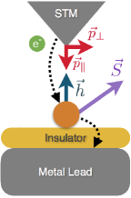
The collective magnetic moment is a good effective description of an atomic aggregate with a large charge-gap. The exchange interaction between the magnetic moment and electrons in the metallic leads is induced by virtual processes where the atomic aggregate acquires (donates) and donates (acquires) an electron from the leads. Such processes induce relaxation and decoherence effects to the magnetic state and allow a charge current to ensue in the presence of a finite applied voltage. If the effective exchange coupling is not too strong, a perturbative treatment allows for the description of the dynamics in terms of a (non-Markovian) master equation for the density matrix of the magnetic moment; the details of the derivation can be found in Ref. (Shakirov et al., 2016).

A simple limit is recovered for a large bias voltage, where the environment becomes memoryless. In this limit, the effect of the leads is simply to perform spin-flips at a constant rate. In case the leads are spin polarized, this yields a net spin transfer. In this Markovian limit the Liouvillian super-operator, $\mathcal{L}$, determining the evolution of the system’s reduced density matrix, $\partial_{t}\rho=\mathcal{L}\left(\rho\right)$, acquires the Lindblad form (Breuer and Petruccione, 2007; de Vega and Alonso, 2017)

$$\mathcal{L}\left(\rho\right)=-i[H,\rho]+\sum_{i}W_{i}\rho W_{i}^{\dagger}-\frac{1}{2}\left\{\rho,W_{i}^{\dagger}W_{i}\right\}$$ (2)

where $W_{i}$, with $i=+,-,z$, are the so called jump operators

$$W_{z}=\sqrt{\frac{\Gamma}{2s}}\tilde{S}_{z};\>W_{+}=\sqrt{\frac{\Gamma}{2s}\frac{1-p}{2}}\tilde{S}_{+};\>W_{-}=\sqrt{\frac{\Gamma}{2s}\frac{1+p}{2}}\tilde{S}_{-}$$ (3)

The tilde “$\,\tilde{\,}\,$” denotes that the quantization axis of the operator is taken along the polarization of the tip. In the two situations treated here, we have $\tilde{S}_{\alpha}=S_{\alpha}$ for the parallel case and $\tilde{S}_{\alpha}=e^{i\frac{\pi}{2}S_{x}}S_{\alpha}e^{-i\frac{\pi}{2}S_{x}}$ for the perpendicular setup. $\Gamma$ is the rate of the quantum jumps, proportional to the absolute value of the applied voltage (see Appendix G of Ref. (Shakirov et al., 2016)).

Under Liouvillian dynamics, the evolution of the density matrix is given by

$$\rho(t)=e^{t\mathcal{L}}\rho(t_{0})=\sum_{i}\exp\left(t\Lambda_{i}\right)X_{i}\text{tr}\left[\tilde{X}_{i}\rho(t_{0})\right]$$ (4)

where $X_{i}$ and $\tilde{X}_{i}$ are respectively left and right eigenvectors of the super-operator corresponding to the eigenvalue $\Lambda_{i}$ and normalized such that $\text{tr}\left[X_{i}\tilde{X}_{j}\right]=\delta_{ij}$. The real part of $\Lambda_{i}$ is non-positive and there is at least one zero eigenvalue $\Lambda_{0}=0$ corresponding to left eigenvector $\tilde{X}_{0}=1$.

Figure 2: Left panel: Phase diagram for $\boldsymbol{p}\parallel\boldsymbol{h}$, plotted for $p\Gamma=1$. Right panels: Average magnetization $\boldsymbol{n}=\left\langle\boldsymbol{S}\right\rangle/s$ shown for representative states of each phase. Stable (unstable) infinite-$s$ steady-states are depicted as black (red) points. Representative trajectories in the $s=\infty$ limit are represented in full colored (pink, green and orange) lines. The steady state and the evolution of the magnetization for $s=20$ are depicted by a blue point and blue dashed line respectively. Parameters: $\text{I}_{\parallel}$ - $h=1,\gamma_{x}=-0.2,\gamma_{y}=-0.3,p\Gamma=0.2$; $\text{II}_{\parallel}$ - $h=1,\gamma_{x}=0.5,\gamma_{y}=-2.5,p\Gamma=1$; $\text{III}_{\parallel}$ - $h=1,\gamma_{x}=-3,\gamma_{y}=-1.5,p\Gamma=1$.

Figure 3: Left panel: Phase diagram for $\boldsymbol{p}\perp\boldsymbol{h}$. Right panel: $\boldsymbol{n}=\left\langle\boldsymbol{S}\right\rangle/s$ shown for states for the different phases. The color codes are the same as in Fig.2. In the middle panel ($\text{I}^{\prime}_{\perp}$), the separatrix separating the two qualitative long-time states of regions $\text{0}_{\perp}$ and $\boldsymbol{\text{I}}_{\perp}$ is depicted in gray. The plots are done for the following set of parameters: $\text{0}_{\perp}$- $h=1,\gamma_{x}=0.1,\gamma_{y}=0.2,p\Gamma=1$;$\text{I}_{\perp}$- $h=1,\gamma_{x}=-2,\gamma_{y}=2.1,p\Gamma=1$;$\text{I'}_{\perp}$- $h=0.2,\gamma_{x}=0.1,\gamma_{y}=1,p\Gamma=1$.

III Steady-state Phase Diagram

In this section, we determine the phase diagram of the model and characterize the different phases according to the qualitative properties of the steady-states. As in equilibrium, non-analyticities in the steady-state observables are only expected once the thermodynamic limit is taken, i.e $N=2s\to\infty$. Since, within the symmetric sector, the total angular momentum is determined by $s=N/2$, the thermodynamic limit corresponds to that of a large classic spin, $s\to\infty$.

To approximate the dynamics of $\rho\left(t\right)$ in the large $s$ limit, we assume an ansatz density matrix of the form $\rho\propto e^{\boldsymbol{m}.\boldsymbol{S}}$, and derive the equation of motion for the vector $\boldsymbol{m}$. Away from phase transition points, this ansatz becomes exact in the $s\to\infty$ limit and allows for higher order corrections in powers of $1/s$. In Appendices A.2 and A.1, we provide the details of the method and show how this approach compares with the standard mean-field approximation (Kilin, 1978; Drummond and Carmichael, 1978; Drummond, 1980; Carmichael, 1999).

From the ansatz parameter $\boldsymbol{m}$, we compute the rescaled magnetization vector $\boldsymbol{n}=\left\langle\boldsymbol{S}\right\rangle/s$ and solve the fixed-point condition $\partial_{t}\boldsymbol{n}=0$ in order to obtain the steady-state magnetization. The fixed-points of the dynamics are classified as attracting (stable), repulsive (unstable), mixed (saddle-points, having at least one attractive and one repulsive direction) or marginal (no attractive or repulsive direction), according to the dynamics in their vicinity. Regarding steady-state properties, different phases are characterized by the number and nature of the fixed-points. A change in the number or nature of the fixed points typically corresponds to non-analyticities of certain observables as well as in the slowest decaying rate towards these points.

We recall that, while all fully-polarized vectors, i.e. $\left|\boldsymbol{n}\right|=1$, correspond to pure states, vectors with $\left|\boldsymbol{n}\right|<1$ may correspond both to pure or mixed states.

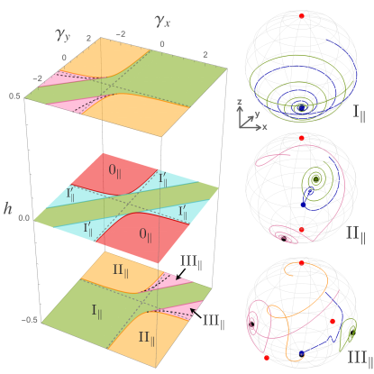
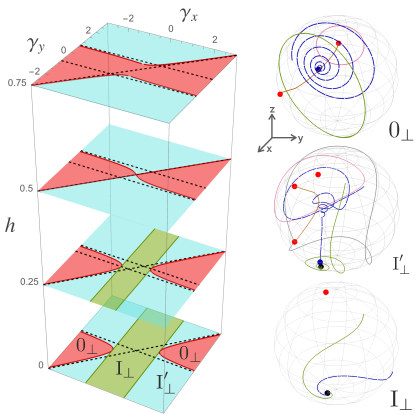
In the following two sub-sections, we study the two cases shown in Fig. 2 and 3, corresponding to an applied field parallel ($\boldsymbol{p}\parallel\boldsymbol{h}$) or perpendicular ($\boldsymbol{p}\perp\boldsymbol{h}$) to the polarization. We qualitatively describe the different phases, as well as the nature of the phase transitions between them based on the steady-state properties and dynamics. The spectral analysis within each phase is relegated to Sec. IV.

The main findings of this section are summarized in Sec. V (see Table 1).

III.1 Parallel polarization

For parallel polarization ($\boldsymbol{p}\parallel\boldsymbol{h}$) [see Fig. 2-(left panel)], there are three stable phases, $\text{I}_{\parallel}$, $\text{II}_{\parallel}$ and $\text{III}_{\parallel}$, in the $\gamma_{x}-\gamma_{y}-h$ parameter space, separated by critical surfaces where phase transitions occur. Regions $\text{0}_{\parallel}$ and $\text{I}^{\prime}_{\parallel}$, arising only at $h=0$, are also critical and correspond either to $\text{I}_{\parallel}\leftrightarrow\text{III}_{\parallel}$ transitions or to transitions between phases $\text{II}_{\parallel}$ with different steady-state symmetries. The critical phases $\text{0}_{\parallel}$ and $\text{I}^{\prime}_{\parallel}$ are similar to some of the phases found in the perpendicular case ($\boldsymbol{p}\perp\boldsymbol{h}$) and we relegate their study for the next subsection. While phases $\text{I}_{\parallel}$, $\text{II}_{\parallel}$ and $\text{III}_{\parallel}$ can be distinguished by their number of fixed points (1,2 and 3), the further division within region $\text{III}_{\parallel}$, depicted as a dashed black line, is obtained by considering steady-state properties at finite-$s$ (see below).

Fig. 2-(right panels) illustrates the dynamics of the average magnetization, $\left\langle\boldsymbol{S}\right\rangle$, within each phase. Pink, green and yellow curves correspond to qualitatively different trajectories obtained by our variational method. Attractive fixed-points are depicted by black dots and the red dots represent unstable or saddle points. An example of the dynamics for a finite-$s$, obtained by exact diagonalization of the Liouvillian, is depicted as blue dashed lines and the steady-state attained in the limit $t\to\infty$ is depicted as blue dots.

Phases

- Region $\text{I}_{\parallel}$ is characterized by a unique stable steady-state located along the $z$-axis. The average magnetization of the steady-state for finite-$s$ approaches the variational ansatz value up to $1/s$ corrections (almost coinciding blue and black points in Fig. 2-$\text{I}_{\parallel}$). The variational and finite-$s$ dynamics (green and blue-dashed lines respectively) yield qualitatively similar results. In addition to the attractive fixed point at the south pole (black dot), an unstable fixed point is located at the north pole (red dot). Saddle points, not present for the choice of parameters of Fig. 2-$\text{I}_{\parallel}$, may appear but do not change the dynamics qualitatively .

- In region $\text{II}_{\parallel}$ (Fig. 2-$\text{II}_{\parallel}$), we find two variational steady-states related by symmetry. For finite-$s$, the degeneracy of the eigenvalues of the Liouvillian is lifted and a unique steady-state emerges (blue dot) whose magnetization approaches the average of the two variational ones. In the variational dynamics, one of the two attractors is attained at large times depending on the initial condition (green and pink lines in Fig. 2-$\text{II}_{\parallel}$); for finite-$s$ (blue dashed line) there are two separated time scales, the initial dynamics approaches one of the variational fixed points and is followed by a decay to the finite-s steady state. We analyze the two time scale dynamics in Sec. IV.3.

- Region $\text{III}_{\parallel}$ has three variational stable fixed points (two related by symmetry and one with $\left\langle\boldsymbol{S}\right\rangle=-s\boldsymbol{e}_{z}$). Which fixed point is realized in the $t\to\infty$ limit depends on the basin of attraction of the initial state. The finite-$s$ dynamics also shows a separation of time-scales, similar to region $\text{II}_{\parallel}$, before the finite-$s$ steady-state is attained.

Phase transitions

We now turn to the description of the phase transitions. Figs. 4 and 5 show the magnetization in the $x$ (left panels) and $z$ (right panels) directions as a function of $\gamma_{x}$ and $h$, for finite values of $s$ (blue and green dots) and for the stable (orange) and unstable (pink) fixed-point of the variational dynamics. Fig. 4 depicts the passage from phase $\text{I}_{\parallel}$ to phase $\text{II}_{\parallel}$, with (upper panels) and without (lower panels) the presence of the intermediate phase $\text{III}_{\parallel}$. Fig. 5 shows a cross section of the phase diagram of Fig. 2-(left panels) obtained by varying $h$ along two vertical lines that cross the $\text{I}_{\parallel}\leftrightarrow\text{III}_{\parallel}$ transition (upper panels) and the $\text{II}_{\parallel}\leftrightarrow\text{II}_{\parallel}$ one (lower panels) that crosses the $\text{0}_{\parallel}$ critical plane.

Figure 4: Upper panels: magnetization for the phase transition $\text{I}_{\parallel}\leftrightarrow\text{III}_{\parallel}\leftrightarrow\text{II}_{\parallel}$ for $h=1,\gamma_{y}=-3,p\Gamma=1$. Lower panels: magnetization for phase transition $\text{I}_{\parallel}\leftrightarrow\text{II}_{\parallel}$ for $h=1,\gamma_{y}=2,p\Gamma=1$. The stable and unstable fixed points are depicted as orange and pink lines respectively.

Figure 5: Upper panels: magnetization at the phase transition $\text{I}_{\parallel}\leftrightarrow\text{III}_{\parallel}$ with $\gamma_{y}=3,\gamma_{y}=1,p\Gamma=1$. Lower panels: magnetization at the phase transition for $\text{II}_{\parallel}\leftrightarrow\text{II}_{\parallel}$ with $\gamma_{y}=3,\gamma_{y}=-3,p\Gamma=1$. The stable and unstable infinite-$s$ results are depicted as orange and pink lines respectively.

Analyzing Figs. 4 and 5, we list the properties of each transition.

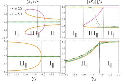
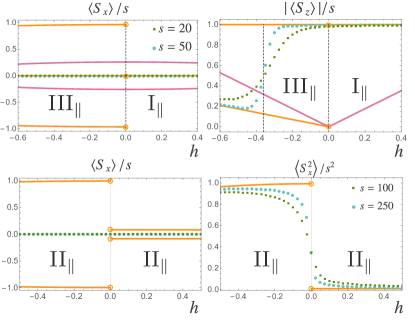
- The transition $\text{I}_{\parallel}\leftrightarrow\text{II}_{\parallel}$ is of second order, with the unique steady-state of $\text{I}_{\parallel}$ giving place to two symmetry broken ones for $\text{II}_{\parallel}$ [see Fig. 4-(lower panels)]. A good order parameter for this transition is $\left\langle S_{z}\right\rangle/s-1$, which vanishes in phase $\text{I}_{\parallel}$ and is non-zero in phase $\text{II}_{\parallel}$.

- At the $\text{II}_{\parallel}\leftrightarrow\text{III}_{\parallel}$ and $\text{III}_{\parallel}\leftrightarrow\text{I}_{\parallel}$ transitions, the quantity $\lim_{s\to\infty}\left\langle S_{z}\right\rangle/s$ computed in the steady-state is analytic as seen in Fig. 4-(upper panels). Analyticity was also observed for all other steady-state observables. Therefore, these transitions only concern dynamic properties.

- A discontinuous steady-state phase transition arises within $\text{III}_{\parallel}$. For finite-$s$, quantum fluctuations select a steady-state with an average magnetization that is either that of the stable fixed-point of $\text{I}_{\parallel}$ or the average of the fixed-points of $\text{II}_{\parallel}$, since these three fixed-points coexist in $\text{III}_{\parallel}$. This scenario of a first order phase transition is similar to that reported in Ref. (Casteels et al., 2017), the only difference being that the phase equivalent to $\text{II}_{\parallel}$ has in Ref. (Casteels et al., 2017) a unique stable fixed-point.

- The transition $\text{I}_{\parallel}\leftrightarrow\text{III}_{\parallel}$ across the plane $h=0$ is of first order. However, since the symmetry is not broken for finite-$s$, the steady-state magnetization is continuous, see Fig. 5.

- The transition $\text{II}_{\parallel}\leftrightarrow\text{II}_{\parallel}$ across the $h=0$ plane is also of first order. The discontinuity of $\left\langle S_{x}^{2}\right\rangle/s^{2}$ is shown in Fig. 5.

III.2 Perpendicular polarization

The case $\boldsymbol{p}\perp\boldsymbol{h}$ shown in Fig. 3-(left panel), has three different phases: $\text{0}_{\perp}$, $\text{I}^{\prime}_{\perp}$ and $\text{I}_{\perp}$. The corresponding dynamics is plotted in Fig. 3-(right panels) with the same color code of Fig. 2. In addition, the gray line in Fig. 3-$\text{I}^{\prime}_{\perp}$ depicts a separatrix curve dividing orbits where variational ansatz has qualitatively different dynamics. Note that, both $\text{0}_{\perp}$ and $\text{I}^{\prime}_{\perp}$ support states that do not relax in the infinite-$s$ limit.

Phases

- Region $\text{0}_{\perp}$ has no variational stable fixed-points. However, the variational method finds a line of marginal fixed-point solutions (brown line) where the eigenvalues of the stability matrix, obtained by linearizing the equations of motion, have a zero real part. This line connects two marginal steady-states that satisfy $\left|\boldsymbol{n}\right|=1$, depicted as red dots on the $z=0$ plane in Fig. 3-$\text{0}_{\perp}$. The dynamics of any initial condition (green and pink lines) follows closed orbits that surround the marginal line. Thus, the asymptotic long-time state of the variational dynamics is recurrent and keeps memory of the initial condition for all times. The existence of recurrent classical solutions was previously identified in (Kilin, 1978; Drummond and Carmichael, 1978; Drummond, 1980; Carmichael, 1999) and recently studied in (Hannukainen and Larson, 2017; Iemini et al., 2017). For the case $\gamma_{x}=\gamma_{y}=0$ and $p=-1$ an explicit solution of the steady-state for finite-$s$ is known (Kilin, 1978; Drummond and Carmichael, 1978; Drummond, 1980).

For finite-$s$, a single unique steady-state (blue dot), with $\left|\left\langle\boldsymbol{S}\right\rangle\right|/s\neq 1$, is attained. This fixed-point corresponds to the unique place along the line of marginal fixed-points where $\left\langle S_{x}\right\rangle=0$, which is consistent with the fact that the finite-$s$ steady-state cannot break the microscopic symmetries.

The finite-$s$ picture emerging from our variational dynamics is the following: finite size corrections destabilize the recurrent variational evolution (valid for $s\to\infty$) and, after a timescale that increases with $s^{-1}$ (see Sec.B), the unique steady-state is attained. Note that, if the initial state is arbitrarily close to one of the marginal fixed points, the evolution to the finite-$s$ steady-state is along the lines of marginal fixed-points found by the variational method. Therefore, including $1/s$ corrections to the variational procedure is expected to lift the degeneracy of the states along the line and yield a unique steady-state that coincided with the finite-$s$ one.

- Region $\text{I'}_{\perp}$ is characterized by a stable fixed-point solution coexisting with recurrent states. A separatrix line ( gray line in Fig. 3-$\text{I}^{\prime}_{\perp}$) separates the region where an initial state attains asymptotically the stable fixed point (e.g. green trajectory) from the region where an initial state yields a recurrent evolution (e.g. pink trajectory). The finite-$s$ evolution (blue dashed line) starting from an initial state in the recurrent region, first follows the variational recurrent evolution and, subsequently, decays towards the unique stable fixed-point.

- Region $\text{I}_{\perp}$ has a single stable steady-state and the same qualitative properties as $\text{I}_{\parallel}$. This region exists only for $h<h_{c}=p\Gamma/2$.

Phase transitions

Figure 6: Magnetization across the $\text{0}_{\perp}\leftrightarrow\text{I}^{\prime}_{\perp}\leftrightarrow\text{I}_{\perp}$ transitions for $h=0.2,\gamma_{y}=-2,p\Gamma=1$. The stable infinite-$s$ steady-state is depicted as orange line.

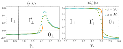
The phase transitions in the perpendicular case can be of two kinds $\text{0}_{\perp}\leftrightarrow\text{I}^{\prime}_{\perp}$ and $\text{I}^{\prime}_{\perp}\leftrightarrow\text{I}_{\perp}$. Fig. 6 shows the magnetization in the $y$ (left panel) and $z$ (right panel) directions as a function of $\gamma_{x}$ for two values of $s$ (blue and green dots) and for the stable fixed-point obtained by the variational ansatz (orange curve). When $h<1/2$, there are two points within a fixed $h$ plane for which the passage from $\text{0}_{\perp}$ to $\text{I}_{\perp}$ can be done directly, without passing by $\text{I}^{\prime}_{\perp}$. As the steady-state properties of phases $\text{I}^{\prime}_{\perp}$ and $\text{I}_{\perp}$ are similar, crossing the transition along these special points will not affect qualitatively the scenario presented in Fig. 6.

- The $\text{0}_{\perp}\leftrightarrow\text{I}^{\prime}_{\perp}$ transition is of first order, with a discontinuous magnetization shown in Fig. 6. However, as there is no stable fixed-point within phase $\text{0}_{\perp}$, this transition seems to escape the Landau paradigm (Hannukainen and Larson, 2017).

- The $\text{I}^{\prime}_{\perp}\leftrightarrow\text{I}_{\perp}$ transition regards only the spectral properties of the Liouvillian and is discussed below. The steady-state magnetization, depicted in Fig. 6 for finite $s$, is continuous across the transition for $s\to\infty$.

IV Steady-State, Spectral and Dynamic Signatures of Non-Equilibrium Phases

In this section, we analyze the spectral and steady-state properties of the phases described in Sec. III. For these quantities, large-$s$ predictions require to go beyond the variational analysis. We achieve this using a Holstein-Primakoff transformation, mapping the spin into a bosonic degree of freedom, which allow a subsequent $1/s$ expansion of the Liouvillian. At leading order, the bosonic Liouvillian is quadratic and thus exactly solvable. Details of the exact solution are given in Appendix C. Analytic predictions obtain in this way are then compared with exact diagonalization results.

The main findings of this section are summarized in columns 4 and 5 of Table 1 and discussed in Sec. V.

IV.1 Holstein-Primakoff transformed Liouvillian

The Holstein-Primakoff (H-P) transformation maps a spin$-s$ into a bosonic degree of freedom. A generalized version of this transformation, which conserves the spin commutation relations, can be obtained by the usual mapping

$$S_{z} =-s+a^{\dagger}a$$ (5)

$$S_{+} =a\sqrt{2s-a^{\dagger}a}$$ (6)

$$S_{-} =\sqrt{2s-a^{\dagger}a}\,a^{\dagger}$$ (7)

followed by a shift in the bosonic operators $a\to a+\sqrt{2s}\frac{\alpha}{\sqrt{1+\bar{\alpha}\alpha}}$ , with $\alpha\in\mathbb{C}$. This generalized H-P mapping allows a systematic $1/s$ development around a spin-coherent state, $\left|\alpha\right\rangle_{c}=e^{\alpha S_{+}}\left|s,-s\right\rangle$, parametrized by $\alpha$, with average magnetization

$$\left\langle\boldsymbol{S}\right\rangle =s\left\{\frac{\alpha+\text{$\bar{\alpha}$}}{1+\bar{\alpha}\alpha},i\frac{\alpha-\bar{\alpha}}{1+\bar{\alpha}\alpha},1-\frac{2}{1+\bar{\alpha}\alpha}\right\}+O\left(\sqrt{s}\right).$$

Inserting the expansion of the spin operators in the Liouvillian and developing in powers of $s$, up to order $s^{0}$, we obtain a quadratic Liouvillian in the bosonic operators, where $H$ can generically be casted in the form

$$H =A^{\dagger}.\boldsymbol{H}.A+A^{\dagger}.\zeta+\zeta^{\dagger}.A+O\left(s^{-1/2}\right)$$ (9)

with $A=\left\{a,a^{\dagger}\right\}^{T}$, the single-particle Hamiltonian $\boldsymbol{H}$ is a $2\times 2$ matrix and $\zeta$ a two-component complex vector. In the same way the jump operator $W_{i}$ can be written as

$$W_{i} =w_{i}^{\dagger}.A+c_{i}$$ (10)

with $w_{i}$ a two-component complex vector and $c_{i}$ a complex constant. The quantities $\boldsymbol{H}$ and $w_{i}$ are of order $s^{0}$ and $\zeta$ and $c_{i}$ are of order $s^{1/2}$. A suitable choice of the shift, $\alpha$, can be used to set to zero the terms proportional to $\zeta$ or $c_{0}$ in the linearized Liouvillian, obtaining an operator with only quadratic terms. The values of $\alpha$ that have this property are those that fulfill fixed-point conditions of the variational and semi-classical dynamics given in Appendix A.1. This step, is thus, equivalent to choose as linearization points the fixed points of the infinite-$s$ equation of motion with $\left|\boldsymbol{n}\right|=1$.

Properties of quadratic bosonic Liouvillians were studied in Ref. (Prosen and Seligman, 2010). We derive some of these results in the Appendix C using an approached similar to that developed in Ref. (Ribeiro and Vieira, 2015) for quadratic fermionic Liouvillians. Using this method, we compute the single particle correlation matrix, $\boldsymbol{\chi}=\left\langle A.A^{\dagger}\right\rangle$, which encodes the properties of the steady-state, the spectral gap, and derive the simple structure of the low energy spectrum.

IV.2 Steady-state

Figure 7: $1/s$ corrections to $\left\langle S_{z}\right\rangle-s$ (left panel) and $S_{E}$ (right panel) with $h=1,\gamma_{y}=2,\Gamma=1/p$.

In this section, we study steady-state properties starting with the parallel polarization case ($\boldsymbol{p}\parallel\boldsymbol{h}$).

For phase $\text{I}_{\parallel}$, there is only one stable solution, $\alpha_{1}$, of the variational equations, thus to leading order in $s$, $\rho_{0}\simeq\left|\alpha_{1}\right\rangle_{c}\left\langle\alpha_{1}\right|_{c}$. Analytic predictions for the steady-state observables to next-to-leading order can be obtained using density matrix $\rho_{0}=\chi_{1}$, where $\chi_{1}$ is the density matrix obtained by linearizing the Liouvillian around $\alpha_{1}$.

For phase $\text{II}_{\parallel}$, at leading order in $s$, $\mathcal{L}$ has two eigenstates with eigenvalues exponentially close to zero that are well approximated by $\rho_{0}=\frac{1}{Z_{0}}\left(\left|\alpha_{1}\right\rangle_{c}\left\langle\alpha_{1}\right|_{c}+\left|\alpha_{2}\right\rangle_{c}\left\langle\alpha_{2}\right|_{c}\right)$, with $Z_{0}=\text{tr}\left(\left|\alpha_{1}\right\rangle_{c}\left\langle\alpha_{1}\right|_{c}+\left|\alpha_{2}\right\rangle_{c}\left\langle\alpha_{2}\right|_{c}\right)$, and $\rho_{1}=\left|\alpha_{1}\right\rangle_{c}\left\langle\alpha_{1}\right|_{c}-\left|\alpha_{2}\right\rangle_{c}\left\langle\alpha_{2}\right|_{c}$, from which only $\rho_{0}$ is a physical density matrix. At next to leading order in $s$, the density matrix is given by $\rho_{0}=\frac{1}{2}\left(\chi_{1}+\chi_{2}\right)$, where $\chi_{1,2}$ are the finite entropy density matrices obtained by linearizing the Liouvillian around $\alpha_{1,2}$, respectively. Since the overlap $\left\langle\alpha_{1}\right.\left|\alpha_{2}\right\rangle_{c}$ is exponentially small in $s$, $\chi_{1}$ and $\chi_{2}$ are exponentially non-overlapping, i.e. $\ln\text{tr}\left(\chi_{1}\chi_{2}\right)\propto-s$. As a consequence, mean values of operators can be approximated by $\text{tr}\left(\rho_{0}O\right)\simeq\frac{1}{2}\left[\text{tr}\left(\chi_{1}O\right)+\text{tr}\left(\chi_{2}O\right)\right]$. The entropy of $\rho_{0}$ is also well approximated by $S_{\text{E}}\simeq\ln 2-\frac{1}{2}\text{tr}\left(\chi_{1}\ln\chi_{1}\right)-\frac{1}{2}\text{tr}\left(\chi_{2}\ln\chi_{2}\right)=\ln 2-\text{tr}\left(\chi_{1}\ln\chi_{1}\right)$, since by symmetry the entropy of $\chi_{1}$ and $\chi_{2}$ are equal.

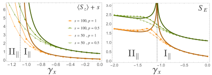
Fig. 7 shows, the $1/s$ corrections to the magnetization $\left\langle S_{z}\right\rangle-s$ and the von Neumann entropy, $S_{\text{E}}=-\text{tr}\left(\rho\ln\rho\right)$, of the steady-state as a function of $\gamma_{x}$, in phases $\text{I}_{\parallel}$ and $\text{II}_{\parallel}$ and across the $\text{I}_{\parallel}\leftrightarrow\text{II}_{\parallel}$ transition. Since in phase $\text{I}_{\parallel}$, the magnetization satisfies $\left\langle S_{z}\right\rangle=-s+\delta S_{z}+O\left(s^{-1}\right)$, the values of $\delta S_{z}=s+\left\langle S_{z}\right\rangle$ for finite-$s$ converge to the analytic predictions obtained using the linearized Liouvillian around the stable steady-state. For the entropy, Fig. 7 shows that the numerical results tend to the analytic predictions as $s\to\infty$. The convergence is much slower around the phase transition point.

At the phase transition, the perturbative expansion is no longer valid and the above estimate breaks down. When the linearized steady-state is a good approximation of the finite-$s$ one, the von Neumann entropy in the $s=\infty$ limit approaches a constant value. The proximity with the critical point where the linearized procedure breaks down, explains the slow convergence with $s$.

For the perpendicular polarization case ($\boldsymbol{p}\perp\boldsymbol{h}$) and in the regions where a stable steady-state is present ($\text{I}_{\perp}$and $\text{I}^{\prime}_{\perp})$, the properties of the steady-state are similar to those of region $\text{I}_{\parallel}$. On the other hand, the recurrent region $0_{\perp}$ has no stable fixed-point to approximate the finite-$s$ steady-state. In this case, as presented below, the entanglement entropy of the finite-$s$ steady state grows as $\ln(s)$. It is tempting to interpret this logarithmic growth as an extension of the argument above for phase $\text{II}_{\parallel}$, where $O\left(s\right)$ degenerate steady-states contribute equally to $S_{\text{E}}$.

IV.3 Spectrum and characteristic time-scales

We now focus on spectrum of the Liouvillian linearized around each steady-state. For the case of a single bosonic mode obtained by $1/s$ expansion of the H-P transformation, the eigenvalues $\Lambda_{n,m}$ of the Liouvillian are given by $\Lambda_{n,m}=i\left(n\lambda-m\bar{\lambda}\right)$, with $m,n\in\mathbb{N}_{0}^{+}$ , where $\lambda$ is a complex number that can be obtained from $\boldsymbol{H}$ and $w_{i}$ (see Appendix C ). Each eigenvalue corresponds to a decaying mode of the dynamics towards the steady-state with a characteristic time scale $\tau=-\left(\text{Re}\Lambda\right)^{-1}$.

Parallel case

Figure 8: Numerical eigenspectrum of $\mathcal{L}$ for regions $\text{I}_{\parallel}$ (left) and $\text{II}_{\parallel}$ (right) and analytical predictions obtained from the linearized Liouvillian around the stable fixed point (light orange) and around the unstable one (light blue). Parameters from Fig.2.

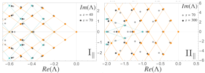
Fig. 8 depicts the spectrum of the Liouvillian $\mathcal{L}$ in $\text{I}_{\parallel}$ and $\text{II}_{\parallel}$ . The gray level coded dots correspond to spectrum of the full Liouvillian for increasing values of $s$. The orange (blue) dots correspond to the spectrum of the linearized Liouvillian around the stable (unstable) fixed points, the orange (blue) lines were drawn to highlight the simple periodic structure of the spectrum.

For the case of Fig. 8-$\text{I}_{\parallel}$, the spectrum is generated by $\lambda=\lambda_{\text{s}}=\sqrt{\left(h+\gamma_{x}\right)\left(h+\gamma_{y}\right)}-\frac{1}{2}i\Gamma p$ (see derivation in Sec. C.3). Note that the agreement between the finite-$s$ spectrum and the linearized one is faster for small values of $\left|\text{Re}\left(\Lambda_{n,m}\right)\right|$. For larger values, we can still observe a convergence to the linearized prediction with increasing $s$. The decay towards the unique steady-state, after the fast decaying modes vanish, is ruled by the two slowest decaying modes depicted in Fig. 8-$\text{I}_{\parallel}$ with a characteristic time-scale $\tau_{0}=\left|\text{Im}\left(\lambda_{s}\right)\right|^{-1}$.

In case of Fig. 8-$\text{II}_{\parallel}$ there are two stable fixed points related by symmetry. Linearizing the Liouvillian around each of these fixed points yields a spectrum that is doubly degenerate. A quasi-degeneracy is also observed in the finite-$s$ spectrum obtained by exact diagonalization with a convergence to the linearized prediction with increasing $s$.

In region $\text{II}_{\parallel}$, the dynamics for finite-$s$ is thus characterized by two different time scales. The first timescale, of order $s^{0}$, is given by $\tau_{0}=\left|\text{Im}\left(\lambda_{s}\right)\right|^{-1}$, with $\lambda_{\text{s}}$ obtained by linearizing the Liouvillian around one of the two symmetry-related stable steady-states. The choice of the particular steady-state depends on which basin of attraction the initial conditions belong to. Within this timescale, the evolution of a finite-$s$ system tends to the infinite-$s$ evolution as the value of $s$ increases. For times $t>\tau_{0}$, the dynamics resolves the degeneracy between the steady-state $\rho_{0}$ and the first excited state $\rho_{1}$ of $\mathcal{L}$ defined in Sec. IV.2 and the decay is dominated by the inverse of the first non-zero eigenvalue $\Lambda_{1}$ of $\mathcal{L}$, $\tau_{1}=-(\text{Re}\Lambda_{\text{1}})^{-1}$. As $\text{Re}\left(\Lambda_{1}\right)$ is exponentially small in $s$, these two timescales become increasingly separated for large $s$ and can be well identified in the dynamics (see Appendix B for more details).

The spectrum of region $\text{III}_{\parallel}$ is thrice degenerate in the infinite-$s$ limit and we also observe convergence as $s$ increases (plot not shown). The dynamics in the region is similar to phase $\text{II}_{\parallel}$ with the exception that now there are three relevant time-scales. The first, $\tau_{0}=\left|\text{Im}\left(\lambda_{s}\right)\right|^{-1}$, determines the convergence to the basin dependent steady-state. One of the two other timescales ($\tau_{1}$ or $\tau_{2}$) corresponds, as in phase $\text{II}_{\parallel}$, to the decay from one of the symmetry related states to the symmetric mixed-state. The other, to the decay between the mixed-symmetric state and a state with $\left\langle\boldsymbol{S}\right\rangle\simeq-s\boldsymbol{e}_{z}$ (as the steady-state of $\text{I}_{\parallel}$). Which eigenvalue, $\Lambda_{1}$ or $\Lambda_{2}$, corresponds to each of these processes depends on what side of the first order transition the system is in.

Interestingly, there is a set of low-lying eigenvalues (blue dots) obtained by exact diagonalization that do not converge to the spectrum of the bosonic Liouvillian linearized around the stable fixed points. Instead, these second set of eigenvalues can be obtained by linearizing the Liouvillian around the unstable fixed-points. This spectrum has a similar structure (blue lines) to that of the stable fixed point but the element with the smallest real part within this set of eigenvalues has a finite negative value, i.e. it is not a steady-state. For the case $\text{I}_{\parallel}$, we obtain $\lambda=\lambda_{\text{uns}}=\sqrt{\left(h-\gamma_{x}\right)\left(h-\gamma_{y}\right)}+\frac{i\Gamma p}{2}$ (see derivation in Sec. C.3) and the cone-like structure is displaced from the real axis by $-\Gamma p$. A convergence to this second set of analytical predictions is also observed in cases $\text{I}_{\parallel}$ and $\text{II}_{\parallel}$.

Therefore, the lower part of the spectrum of the full Liouvillian, that rules the long-time dynamics, is an overlap of the spectra of linearized Liouvillians around both stable and unstable fixed points. Thus, in addition to the characteristic timescales determined by the stable fixed-points, the long-time dynamics also carries information about the unstable fixed points.

We now focus on the spectrum at the phases transitions of the parallel case. As noticed before, there are three kinds of steady-state phase transitions in the system: two first order, one with coexisting stable fixed points ($\text{I}_{\parallel}\leftrightarrow\text{III}_{\parallel}\leftrightarrow\text{II}_{\parallel}$) and one with no coexistence ($\text{II}_{\parallel}\leftrightarrow\text{II}_{\parallel}$), and a second order phase transition ($\text{I}_{\parallel}\leftrightarrow\text{II}_{\parallel}$). The $\text{I}_{\parallel}\leftrightarrow\text{III}_{\parallel}\leftrightarrow\text{II}_{\parallel}$ transition is hard to locate numerically and an analytical treatment of the spectral properties beyond the heuristic picture given above requires a non-perturbative treatment that is out of the scope of this work. The transition $\text{II}_{\parallel}\leftrightarrow\text{II}_{\parallel}$ is realized passing by the $0_{\parallel}$ critical plane in Fig. 2-(left panel); the spectral and the steady-state properties of this phase are similar to those of phase $0_{\perp}$ and will be analyzed in the next section.

Figure 9: Left panel: Real part of the smallest eigenvalues at the transition $\text{I}_{\parallel}\leftrightarrow\text{II}_{\parallel}$ as a function of $s$, parameters of Fig.2. Inset: von Neumann entropy of the steady-state as function of $s$. Right: Spectrum of $\mathcal{L}_{\text{}}$ at the $\text{I}_{\parallel}\leftrightarrow\text{II}_{\parallel}$ transition, gray dots represent numeric values from $s=60$ up to $s=500$ and the lines are trajectories as function of $s$.

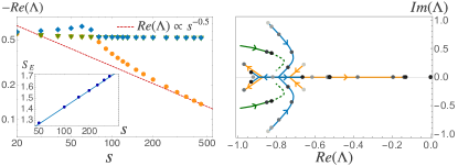
The spectrum at the $\text{I}_{\parallel}\leftrightarrow\text{II}_{\parallel}$ critical point is depicted in Fig. 9. As $s$ increases, a larger number of eigenvalues approaches zero following a process sketched in Fig. 9-(right panel): for increasing s (see arrows), two complex conjugate eigenvalues meet and become real; after that one eigenvalue approaches zero. The behavior of the first eigenvalue of the Liouvillian that converges to $0$ with $s$ is given in Fig. 9-(right panel), showing $\Lambda_{1}\propto s^{-\nu}$ with $\nu\simeq 0.5$. The entropy of the finite-$s$ steady-state is given in the inset of Fig. 9-(left panel). The scaling seems to be logarithmic in $s$, i.e. $S_{\text{E}}\propto\ln\left(s\right)$. Away from the phase transition points, all steady-states have a finite entropy in the infinite $s$ limit.

Perpendicular case

The spectrum and dynamics of the magnetization and the entropy in phase $\text{I}_{\perp}$, is similar to that of phase $\text{I}{}_{\parallel}$ in the previous section. Therefore, we refer the reader to the discussion of phase $\text{I}{}_{\parallel}$ (above) for the physical understanding of that phase.

Figure 10: Left panel: Real part of the smallest eigenvalues as a function of $s$ in region $\text{0}_{\perp}$, parameters of Fig.2; Inset: von Neumann entropy as function of $s$. Right panel: Spectrum of $\mathcal{L}$ for region $0_{\perp}$ , light (dark) gray dots represent numeric values for $s=100$ ($s=300$), the orange and blue dots are obtained by linearizing the dynamics around the two marginal infinite-$s$ fixed-points located on the sphere.

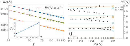
Phases $\text{0}_{\perp}$ and $\text{I}^{\prime}_{\perp}$ allow for recurrent states in the infinite-$s$ limit with a time-independent amplitude and frequency which depend on the initial condition. In the $s\to\infty$ limit, this corresponds to a spectrum of $\mathcal{L}$ with an accumulation of points on the imaginary axis. This property, recently studied in Ref. (Iemini et al., 2017), is shown in Fig. 10 for the case of a point in region $\text{0}_{\perp}$. For finite-$s$ (see Fig. 10-right panel), we observe that some eigenvalues indeed approach the imaginary axis, and, when sufficiently close to the imaginary axis, fall along lines predicted for the marginal fixed points of the linearized Liouvillian. In this phase, the Liouvillian gap $\Lambda_{1}$ and the real part of the first few Liouvillian eigenvalues ($\Lambda_{2}$, $\Lambda_{3}$,…) vanish as $s^{-1}$ (see Fig. 10-left panel).

This implies that in phase $\text{0}_{\perp}$, the approach to the unique finite-$s$ steady state is done with a rate of the order of $s^{-1}$. The entropy of the finite-$s$ steady-state increases logarithmically with $s$ (inset of Fig. 10 - blue dots). In the same inset we compare the entropy of state chosen by our variational procedure (blue line) in Sec. III.2 and find a remarkable agreement (no fitting performed).

The spectrum in phase $\text{I}^{\prime}_{\perp}$ (not shown) is a direct overlap of the spectra of $\text{0}_{\perp}$ and $\text{I}{}_{\perp}$ . Properties of the finite-$s$ steady-state are always well approximated by a quadratic Liouvillian, linearized around the stable fixed point of $\text{I}^{\prime}_{\perp}$.

V Classification of steady-state phases

Description		Abbreviation	Region	Spectral Gap	S.S. Entropy
Non-Critical
	Non-Degenerate	nCnD	$\text{I}_{\parallel},\text{I}_{\perp}$	$\Delta\sim s^{0}$	$S_{E}\sim s^{0}$
	Degenerate - Symmetric	nCDS	$\text{II}_{\parallel}$	$\ln\Delta\sim-s$	$S_{E}\sim s^{0}$
	Degenerate - Non-Symmetric	nCDnS	$\text{III}_{\parallel}$	$\ln\Delta\sim-s$	$S_{E}\sim s^{0}$
Critical
	Non-Recurrent	CnR	$\text{I}_{\parallel}\leftrightarrow\text{II}_{\parallel}$	$\Delta\sim s^{-\frac{1}{2}}$	$S_{E}\sim\ln s$
	Coexistence	CC	$\text{I'}_{\perp}$,$\text{I}^{\prime}_{\parallel}$	$\Delta\sim s^{-1}$	$S_{E}\sim s^{0}$
	Recurrent	CR	$\text{0}_{\perp}$,$\text{0}_{\parallel}$	$\Delta\sim s^{-1}$	$S_{E}\sim\ln s$

Table 1: Classification of steady-state phases.

We can now establish a complete classification of the different phases of the model. A summary of the following discussion and acronyms table is presented in Tab. 1 and should be understood as the main result in our paper.

We start by classifying the different systems in two major classes: non-critical system (NCS), where the number of zero eigenvalues of the Liouvillian operator is finite for $s\to\infty$; and critical systems (CS) that have a spectrum where an infinite number of eigenvalues approaches the imaginary axis as $s\to\infty$.

NCS correspond to the phases $\text{I}_{\parallel}$, $\text{II}_{\parallel}$, $\text{III}_{\parallel}$ and $\text{I}_{\perp}$. For these systems, the spectrum is well approximated by a linearized bosonic Liouvillian obtained after a Holstein-Primakoff transformation around the (stable and unstable) fixed points of the infinite-$s$ dynamics. Each stable point in the dynamics, $\alpha_{i=1,2,3}$, corresponds to a zero eigenvalue on the Liouvillian in the $s\to\infty$ limit with an eigenvector that is well approximated by the density matrix $\rho\simeq\left|\alpha_{i}\right\rangle_{c}\left\langle\alpha_{i}\right|_{c}$, with $\left|\alpha_{i}\right\rangle_{c}$ a spin coherent state. In NCS phases with more than one infinite-$s$ steady-state, the dynamics follows the two time-scale paradigm observed in phases $\text{II}_{\parallel}$, $\text{III}_{\parallel}$. This corresponds to a first decay towards the infinite-$s$ state in the basin of attraction of the initial point, with a time scale of order $s^{0}$, and a second decay to the finite-$s$ steady-state, with a time scale that diverges exponentially as $s$ increases. Observables, such as the steady-state magnetization and entropy, can be obtained, at every order in $s$, by systematically computing $1/s$ corrections to the leading order linearized Liouvillian. In particular, the von Neumann entropy is finite in the infinite-$s$ limit.

NCS systems can be divided into three sub-classes: non-degenerate (nCnD), with unique single steady-state ($\text{I}_{\parallel},\text{I}_{\perp}$); degenerate-symmetric (nCDS) and degenerate-nonsymmetric (nCDnS) where more than one steady state exist ($\text{II}_{\parallel}$ and $\text{III}_{\perp}$ respectively).

- For nCDS phases, a pair of symmetry broken steady-states becomes exponentially degenerate, $\Delta\sim\exp(-s)$, in the infinite-$s$ limit. Because the states break the symmetry of the underlying Liouvillian in the infinite-$s$ limit, the finite-$s$ steady-state is well approximated by a symmetric combination of the two infinite-$s$ states and we say that the transition $\text{I}_{\parallel}\leftrightarrow\text{II}_{\parallel}$ is of second order.

- nCDnS phases can encompass multiple pairs of symmetry broken steady-states and symmetric states. All steady-states are exponentially degenerate in the infinite-$s$ limit, however in order to compute which of the steady-states is realized for finite $s$, a non-perturbative calculation in $s$ is needed that goes beyond the scope of the current work.

CS are represented in this work by regions $0_{\perp}$, $\text{I}^{\prime}_{\perp}$ and by the phase transition planes, including: $\text{0}_{\parallel}$, $\text{I}^{\prime}_{\parallel}$ and the transitions lines $\text{I}_{\parallel}\leftrightarrow\text{II}_{\parallel}$. These can be divided into three sub-classes: recurrent (CR) with all the initial states displaying recurrent behavior ($\text{0}_{\perp}$,$\text{0}_{\parallel}$), coexistence (CC) whose properties depend on the initial state ($\text{I'}_{\perp}$,$\text{I}^{\prime}_{\parallel}$) and non-recurrent (CnR) where a (likely infinite) number of eigenvalues vanish ($\text{I}_{\parallel}\leftrightarrow\text{II}_{\parallel}$).

- CR have a massive degenerate spectrum with non-zero imaginary parts, therefore allowing for recurrent dynamics in the infinite-$s$ limit. While the infinite-$s$ limit does not include a stable-steady state, our variational approach, together with symmetry considerations, can be used to predict both the magnetization and the entropy to leading order in $s$. In this phase, we have that $\lim_{s\to\infty}\left\|\left\langle\boldsymbol{S}\right\rangle\right\|/s<1$ and the von Neumann entropy diverges logarithmically with $s$.

- In CC phases a stable steady state may still exist. In this case the degenerate spectrum coexists with a regular one that is well approximated, as for NCS, by linearizing the Liouvillian around the stable fixed-point. Moreover, the finite-$s$ steady-state are well approximated by those obtained perturbatively from the linearized Liouvillian. This implies that steady-state observables have a convergent $1/s$ expansion and that the entropy of the steady-state is finite in the infinite-$s$ limit.

- For CnR systems, eigenvalues approach zero with a spectral gap that vanishes as a power law. Here, the fitted numerical value is compatible with a mean-field exponent $s^{-1/2}$. This, together with the perturbative results obtained in region $\text{I}_{\parallel}$, suggests that the approach to the steady-state for a generic observable, $\left\langle O\left(t\right)\right\rangle-\left\langle O\left(\infty\right)\right\rangle$, follows a scaling function of the from $s^{-\frac{1}{2}}\Phi\left(\left|\lambda\right|t,\left|\lambda\right|^{2}s^{\frac{1}{2}}\right)$, where $\lambda$ is the eigenvalue of the linearized problem that vanishes at the transition. Assuming a scaling hypothesis, this implies a $t^{-2}$ power law relaxation at the infinite-$s$ limit. However, with the system sizes available to us, we were not able to numerically confirm this prediction. For a CnR, the steady-state entropy is observed to grow logarithmically with increasing $s$.

Although our classification focuses only on the properties of stable and marginal steady-states, we have also shown that the low-lying spectrum of the Liouvillian operator in the large $s$ limit cannot be reproduced only by analyzing the stable fixed points. Instead, the spectrum is obtained as a superposition of two sets of eigenvalues, coming from the stable and unstable fixed points. Since these eigenvalues with a small real part rule the decay to the steady-state at large times, the decay rates also carry information about the unstable fixed points. Such understanding is relevant for experimental setups aimed at studying the characteristic timescales described in Sec. IV.3.

VI Conclusion

In summary, we present a detailed analysis of the LMG model, featuring a collective spin system, in the presence of a Markovian dissipative environment. Motivated by recent prototypes of engineered atomic spin devices we focus on two polarization cases. Our analysis is also of interest to other variants of the dissipative LMG model that have previously been studied in the contexts of quantum optics and cold atomic setups. By employing a variational approach, as well as a $1/s$ perturbative method, we are able to systematically study the model. Despite its apparent simplicity, this model exhibits a rich phase diagram where different phases are shown to possess qualitatively different steady-state and dynamical properties. We identify a number of different phases and provide a tentative classification with terms of their spectral and steady-state properties (see Tab. 1).

One of the open issues, not addressed in the present work, is to understand the nature of the coexisting region near first order phase transitions. Detailed studies (Dombi et al., 2013; Mavrogordatos, 2017) have already reveled some of the properties of distribution functions near the transition. However, in the coexisting region, a criterion to predict which fixed point is realized at finite $s$, similar to Maxwell’s construction for equilibrium first order phase transitions (Callen, 1998), is still lacking.

Appendix A Equations of Motion in the Large $s$ Limit

In this section, we present the details of a derivation of the semi-classical equations of motion of the model. We do this in the next two sub-sections in two slightly different ways. The first is the usual semi-classical analysis. The second method consists of approximating the dynamics by constraining the possible states within a family of variational density matrices. To treat both parallel and perpendicular cases at the same time, in this section, we assume that the Hamiltonian and the jump operators are generically given by

$$H =-\sum_{\alpha}\left(h^{\alpha}S_{\alpha}+\frac{1}{2s}\gamma^{\alpha}S_{\alpha}^{2}\right)$$ (11)

$$W_{i} =\frac{1}{\sqrt{2s}}\sum_{\alpha}\eta_{i}^{\alpha}S_{\alpha}$$ (12)

where $h^{\alpha=x,y,z}$ and $\gamma^{\alpha}$ are real and $\eta_{i}^{\alpha}$ are complex parameters.

A.1 Semi-classical dynamics

A close set of equations of motion in the semi-classical limit is obtained assuming that, for a typical state, $\left\langle S_{\alpha}S_{\beta}\right\rangle=\left\langle S_{\alpha}\right\rangle\left\langle S_{\beta}\right\rangle+O\left(s^{1}\right)$. Assuming this factorization in the equations of motion for the magnetization

$$\partial_{t}\left\langle S_{\beta}\right\rangle =\text{tr}\left[S_{\beta}\mathcal{L}\left(\rho\right)\right]$$ (13)

one obtains the semi-classical equations of motion for the quantity $n_{\alpha}=\frac{1}{s}\left\langle S_{\alpha}\right\rangle$:

$$\partial_{t}n_{\beta} =\sum_{\alpha\gamma}\varepsilon_{\alpha\beta\gamma}h_{\alpha}n_{\gamma}+\sum_{\alpha\gamma}\varepsilon_{\alpha\beta\gamma}\gamma_{\alpha}n_{\alpha}n_{\gamma}$$

$$-\sum_{i,\alpha\alpha\text{'}\gamma}\frac{1}{2}\varepsilon_{\alpha\beta\gamma}\text{Im}\left[\bar{\eta}_{i}^{\alpha^{\prime}}\eta_{i}^{\gamma}\right]n_{\alpha}n_{\alpha}$$ (14)

where $\varepsilon_{\alpha\beta\gamma}$ is the anti-symmetric tensor.

The stability of the fixed-points of the semi-classical dynamics, i.e. points obeying $\partial_{t}n_{\beta}=0$, is obtained by linearizing the equations of motion in their vicinity

$$\partial_{t}\delta n_{\beta} =M\left(n_{\beta}^{*}\right)\delta n_{\beta},$$

where $n_{\beta}^{*}$ is the value of the fixed-point and $\delta n_{\beta}=n_{\beta}-n_{\beta}^{*}$.

Besides the trivial fixed point with $\left|\boldsymbol{n}\right|=0$, which is found to be generically unstable, all the other fixed points found have $\left|\boldsymbol{n}\right|=1$.

A.2 Variational density matrix

Here we detail the variational approach employed in the main text. The results of this approach only differ from those in the previous section for phase $0_{\perp}$ and $\text{I'}_{\perp}$ , where it allows to find a line of variational steady-states to which the magnetization vector of the finite-$s$ steady-state belongs.

The variational states are parameterized by:

$$\rho\left(\boldsymbol{m}\right) =\frac{e^{\boldsymbol{m}.\boldsymbol{S}/s}}{Z_{\boldsymbol{m}}}$$ (15)

with $Z_{\boldsymbol{m}}=\text{tr}\left[e^{\boldsymbol{m}.\boldsymbol{S}/s}\right]$. This family of states includes thermal states of Hamiltonian that are linear in $\boldsymbol{S}$. Within this family, expectation values $\left\langle S_{\alpha}\right\rangle$ and $\left\langle S_{\alpha}S_{\beta}\right\rangle$ are given by

$$\left\langle\boldsymbol{S}\right\rangle =\boldsymbol{R}.\left\langle\boldsymbol{S}\right\rangle_{z}$$ (16)

$$\left\langle\boldsymbol{S}.\boldsymbol{S}^{T}\right\rangle =\boldsymbol{R}.\left\langle\boldsymbol{S}.\boldsymbol{S}^{T}\right\rangle_{z}.\boldsymbol{R}^{T}$$ (17)

where $\left\langle...\right\rangle_{z}=\text{tr}\left[...e^{\left|\boldsymbol{m}\right|S^{z}/s}\right]/\text{tr}\left[e^{\left|\boldsymbol{m}\right|S^{z}/s}\right]$ and $\boldsymbol{R}$ is a rotation matrix chosen such that $\boldsymbol{m}=\left|\boldsymbol{m}\right|\boldsymbol{R}.\boldsymbol{e}_{z}$. In the large $s$ limit these expressions simplify to

$$\left\langle\boldsymbol{S}\right\rangle/s =L\left(m\right)\frac{\boldsymbol{m}}{m}$$ (18)

$$\left\langle\boldsymbol{S}.\boldsymbol{S}^{T}\right\rangle/s^{2} =G(m)\boldsymbol{m}.\boldsymbol{m}^{T}+\frac{L(m)}{m}\boldsymbol{1}$$ (19)

where

$$L\left(x\right) =\coth\left(x\right)-\frac{1}{x}$$ (20)

$$G(x) =\frac{x^{2}-3x\coth(x)+3}{x^{4}}$$ (21)

Replacing this expressions in the equations of motion one obtains

$$\partial_{t}\left[m_{\beta}\frac{L\left(m\right)}{m}\right] =Y_{\beta}$$ (22)

with

$$Y_{\beta} =\sum_{\alpha\gamma}\epsilon_{\alpha\beta\alpha^{\prime}}h_{\alpha}\frac{L(m)}{m}m_{\alpha^{\prime}}+\sum_{\alpha\alpha\text{'}\gamma}\left[\frac{1}{2}\epsilon_{\alpha\beta\alpha^{\prime}}\left(\gamma_{\alpha}-\gamma_{\alpha^{\prime}}\right)\right.$$

$$+\left.\frac{i}{4}\sum_{i}\left(\bar{\eta}_{i}^{\alpha^{\prime}}\eta_{i}^{\gamma}\varepsilon_{\alpha\beta\gamma}-\bar{\eta}_{i}^{\gamma}\eta_{i}^{\alpha}\varepsilon_{\alpha^{\prime}\beta\gamma}\right)\right]\times$$

$$\left[G(m)m_{\alpha}m_{\alpha\text{'}}+\frac{L(m)}{m}\delta_{\alpha\alpha^{\prime}}\right]$$ (23)

Steady-states must satisfy the condition $\sum_{\beta}Y_{\beta}m_{\beta}=0$. For $Y_{\beta}\neq 0$ this implies: $\left|\boldsymbol{m}\right|\rightarrow\infty$ (fully polarized state) or $\sum_{i,\alpha\gamma}\varepsilon_{\alpha\beta\gamma}\left(\bar{\eta}_{i}^{\alpha}\eta_{i}^{\gamma}-\bar{\eta}_{i}^{\gamma}\eta_{i}^{\alpha}\right)=0$ for all $\beta$. Since the second condition is not verified in either models, steady-states must be fully polarized and the equations for steady-states for $\hat{\boldsymbol{m}}=\boldsymbol{m}/\left|\boldsymbol{m}\right|$ reduce to those of $\boldsymbol{n}$ in the last section, for $\left|\boldsymbol{n}\right|=1$. Therefore, for fully polarized steady-states both approaches coincide. We may also have solutions satisfying $Y_{\beta}=0$. Although a general analytical treatment of the phase diagram of these solutions is beyond this paper’s scope, we propose that the existence of these solutions lead to the recurrent regions observed. In general, a solutions of $Y_{\beta}=0$ will be a continuous line of marginal points connecting the marginal (or saddle) steady-states obtained semi-classically. In this paper, such marginal line only occurs for $\boldsymbol{p}\perp\boldsymbol{h}$ and in the plane $z=0$

Figure 11: Dynamics for $\boldsymbol{p}\parallel\boldsymbol{h}$: Time evolution of $\left\langle S_{y}\right\rangle/s$ (upper panels) and von Neumann entropy $S_{\text{E}}$ (lower panels) of an initial state polarized along the $y$ direction, for different values of $s$. The parameters are those of Fig.2.

Figure 12: Dynamics for $\boldsymbol{p}\perp\boldsymbol{h}$ : Time evolution of $\left\langle S_{x}\right\rangle/s$ (upper panels) and von Neumann entropy $S_{\text{E}}$ (lower panels) of an initial state fully polarized along the $x$ direction for different values of $s$. Parameters of Fig.2.

Appendix B Dynamics for finite-s

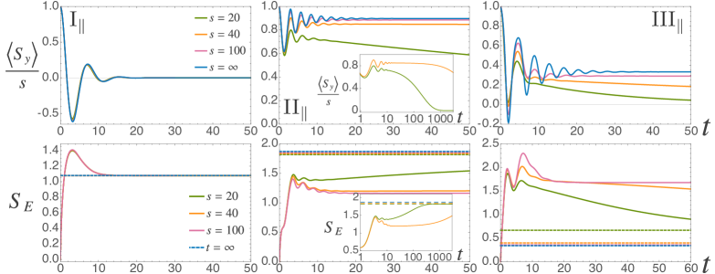
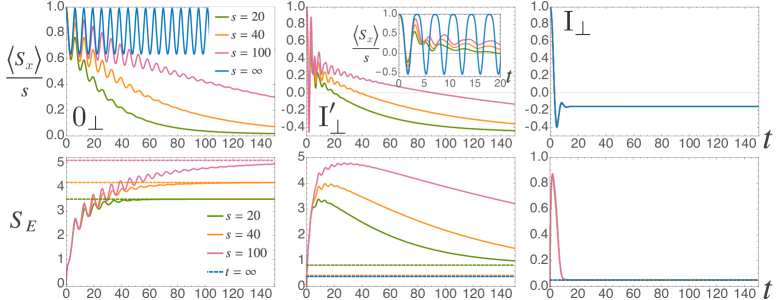
In this section we present some helpful simulations of the magnetization dynamics for finite-$s$ and all regions of the phase diagram. Figs. 11 and 12 show the long time dynamics of a state initially polarized along the $y$ and $x$ direction, respectively, for different spins ($s=20,40,100$).

In parallel case, Fig. 11, we highlight the visible separation of timescales in region $\text{II}{}_{\parallel}$(center panels), first a decay towards the mixed-symmetric state, followed by an exponential decay towards the true steady-state. Unfortunately, the same separation between the three timescales of region $\text{III}{}_{\parallel}$ is not so clear. The $s$ scaling convergence towards the infinite-$s$ magnetization dynamics (depicted as blue full line) and its entropy (blue dashed lines) shows that the variational approach correctly captures the dynamics in the large $s$ limit.

Similarly to the parallel case, the variational approach also captures the dynamics in the large $s$ limit perpendicular case Fig. 12, even when no stable steady-state exists. As discussed in Sec. IV.3 the finite-$s$ steady-state in phase $\text{I}^{\prime}_{\perp}$ is well approximated by the unique stable steady-state at infinite-$s$ even though the short time dynamics suggests a recurrent regime. In Fig. 12-(center) we plot the recurrent magnetization dynamics (upper plot) as blue full line and the entropy of the stable steady-state as dashed blue line (lower plot).

A similar situation occurs in region $\text{0}{}_{\perp}$(Fig. 12-left) with the finite-$s$ steady-state being in the variational line with $\left\langle S_{x}\right\rangle=0$.

Appendix C The Linearized Lindblad Operator

C.1 Steady-state

In this section we derive explicit expressions for the steady-state of a linearized Lindblad operator. The presentation is done in a generic way such that the approach can be used for more than one species of bosons, in which case $A=\left\{a_{1},a_{2},...,a_{n},a_{1}^{\dagger},a_{2}^{\dagger},...,a_{n}^{\dagger}\right\}^{T}$.

As for the case of fermions (Prosen, 2008; Ribeiro and Vieira, 2015), it is useful to consider the single-body density matrix $\boldsymbol{\chi}=\left\langle A.A^{\dagger}\right\rangle$. The particular choice of the value of $\zeta$ and $\bar{w}_{0}$ in the Sec. IV leads to the the vanish of the linear terms in $a$ and $a^{\dagger}$ , therefore we consider that $H=A^{\dagger}.\boldsymbol{H}.A$, where single-particle Hamiltonian is a $2n\times 2n$ matrix respecting: $\boldsymbol{H}^{\dagger}=\boldsymbol{H}$ and $\hat{\boldsymbol{H}}=\boldsymbol{S}\boldsymbol{H}^{T}\boldsymbol{S}$, with $\boldsymbol{S}=\left(\begin{array}[]{cc}&\boldsymbol{1}\\ \boldsymbol{1}\end{array}\right)$, and $W_{i}=w^{\dagger}.A$, where $w$ is a $\mathbb{C}$-valued vector with $2n$ components.

Under these assumptions the steady-state is Gaussian with a vanishing first moment $\left\langle A\right\rangle=0$. Thus, the second moment matrix $\boldsymbol{\chi}$ completely characterizes the steady state density matrix. This can be seen explicitly for a density matrix of the form $\rho_{0}=e^{-\Omega_{0}}/Z_{0}$, with $Z_{0}=\text{tr}\left(e^{-\Omega_{0}}\right)$ and $\Omega_{0}=\frac{1}{2}A^{\dagger}.\boldsymbol{\Omega}_{0}.A$ where $\boldsymbol{\Omega}_{0}$ is Hermitian, $\boldsymbol{\Omega}_{0}^{\dagger}=\boldsymbol{\Omega}_{0}$, and particle-hole symmetric, $\hat{\boldsymbol{\Omega}}_{0}=\boldsymbol{S}\boldsymbol{\Omega}_{0}^{T}\boldsymbol{S}$. In which case the single-body density matrix is explicitly given by

$$\boldsymbol{\chi}_{0} =-n_{b}\left(-\boldsymbol{J}.\boldsymbol{\Omega}_{0}\right)\boldsymbol{J}$$ (24)

with $n_{b}\left(z\right)=\frac{1}{e^{z}-1}$ the Bose function and $\boldsymbol{J}=\left(\begin{array}[]{cc}\boldsymbol{1}\\ &-\boldsymbol{1}\end{array}\right)$.

Considering the adjoint of $\mathcal{L}$, $\mathcal{L}^{\text{ad}}=\mathcal{L}^{\dagger}$, defined as $\text{tr}\left[O\mathcal{L}\left(\rho\right)\right]=\text{tr}\left[\mathcal{L}^{\text{ad}}\left(O\right)\rho\right]$, for the linearized Lindblad operator the equation of motion $\partial_{t}A.A^{\dagger}=\mathcal{L}_{\text{lin}}^{\text{ad}}\left(A.A^{\dagger}\right)$ can be written as

$$\partial_{t}A.A^{\dagger}= -i\left[\boldsymbol{K}.A.A^{\dagger}-A.A^{\dagger}.\boldsymbol{K}^{\dagger}\right]+\boldsymbol{J}.\boldsymbol{N}.\boldsymbol{J}$$ (25)

where we defined

$$\boldsymbol{K}= \boldsymbol{J}.\left(\boldsymbol{H}-i\boldsymbol{\Gamma}\right)$$ (26)

$$\boldsymbol{N}= \sum_{\mu}w_{\mu}.w_{\mu}^{\dagger},$$ (27)

and

$$\boldsymbol{\Gamma}= \frac{1}{2}\left(\boldsymbol{N}-\hat{\boldsymbol{N}}\right)$$ (28)

$$\boldsymbol{M}= \frac{1}{2}\left(\boldsymbol{N}+\hat{\boldsymbol{N}}\right)$$ (29)

Taking the mean value with respect to some density matrix $\left\langle...\right\rangle=\text{tr}\left[...\rho\right]$, we obtain the equation of motion for the single-body density matrix given by

$$\partial_{t}\boldsymbol{\chi}= -i\left[\boldsymbol{K}.\boldsymbol{\chi}-\boldsymbol{\chi}.\boldsymbol{K}^{\dagger}\right]+\boldsymbol{J}.\boldsymbol{N}.\boldsymbol{J}$$ (30)

A solution for the steady-state $\partial_{t}\boldsymbol{\chi}=0$ can be given explicitly as

$$\boldsymbol{\chi}_{\infty}= -i\sum_{\alpha\beta}\left|\alpha\right\rangle\frac{\left\langle\tilde{\alpha}\right|\boldsymbol{J}.\boldsymbol{N}.\boldsymbol{J}\left|\tilde{\beta}\right\rangle}{\lambda_{\alpha}-\bar{\lambda}_{\beta}}\left\langle\beta\right|$$ (31)

where $\left|\alpha\right\rangle$ and $\left\langle\tilde{\alpha}\right|$, with $\left\langle\tilde{\alpha}\right.\left|\beta\right\rangle=\delta_{\alpha\beta}$, are right and left eigenvectors of the operator $\boldsymbol{K}$ which can be decomposed as $\boldsymbol{K}=\sum_{\alpha}\left|\alpha\right\rangle\lambda_{\alpha}\left\langle\tilde{\alpha}\right|$. It is worth noting that the particle-hole anti-symmetry $\boldsymbol{K}$, i.e. $\hat{\boldsymbol{K}}\equiv\boldsymbol{S}\boldsymbol{K}^{T}\boldsymbol{S}=-\boldsymbol{K}^{\dagger}$, implies that the eigenvectors of $\boldsymbol{K}$ appear in pairs: $\left|\alpha\right\rangle$ with eigenvalue $\lambda_{\alpha}$ and $\boldsymbol{S}\left|\bar{\alpha}\right\rangle$ with eigenvalue $-\bar{\lambda}_{\alpha}$.

Higher moments of $\rho_{0}$ can be completely determined by $\boldsymbol{\chi}_{0}$. For example, the entanglement entropy is given by

$$S =\text{tr}\left[\boldsymbol{\chi}_{\infty}\boldsymbol{J}\ln\left(\boldsymbol{\chi}_{\infty}\right)\right]$$

for such quadratic bosonic model. This expression can be computed from the eigenvalues of $\boldsymbol{\chi}_{0}\boldsymbol{J}$ (or of $\boldsymbol{J}\boldsymbol{\Omega}_{0}$) that can be diagonalized by a symplectic transformation $\left(\boldsymbol{J}\boldsymbol{U}\right)\boldsymbol{\chi}_{0}\boldsymbol{J}\left(\boldsymbol{J}\boldsymbol{U}^{\dagger}\right)=\boldsymbol{D}\boldsymbol{J}$, where $\boldsymbol{D}=\boldsymbol{S}\boldsymbol{D}\boldsymbol{S}$ is a diagonal matrix and $\boldsymbol{U}^{\dagger}\boldsymbol{J}\boldsymbol{U}=\boldsymbol{J}$.

C.2 Spectrum and eigenstates of the Linearized Lindblad Operator

In this section, we obtain the spectrum and eigenstates of the linearized Lindblad operator by acting on the steady-state with a set of eigen-operators of $\left[\mathcal{L}_{\text{lin}},...\right]$. We assume at first that $\zeta$ and $\bar{w}_{0}$ are non-zero to see what are the implications and set them to zero later. As for the last section, the formalism is generic and can be used in the case there are several species of bosons.

For the following treatment it is helpful to write the Lindblad operator in the form

$$\mathcal{L}_{\text{lin}} =-\frac{i}{2}\boldsymbol{\mathfrak{a}}^{\dagger}\left[\begin{array}[]{cc}\boldsymbol{H}-i\boldsymbol{M}&i\hat{\boldsymbol{N}}\\ i\boldsymbol{N}&-\boldsymbol{H}-i\boldsymbol{M}\end{array}\right]\boldsymbol{\mathfrak{a}}+i\frac{1}{2}\text{tr}\left(\boldsymbol{K}\right)$$ (34)

with

$$\boldsymbol{\mathfrak{a}} =\left\{a_{1}\otimes 1,a_{2}\otimes 1,...,a_{1}^{\dagger}\otimes 1,...,1\otimes a_{1}^{T},...,1\otimes a_{1}^{\dagger T},...\right\}^{T}$$ (35)

Since $\boldsymbol{\mathfrak{a}}.\boldsymbol{\mathfrak{a}}^{\dagger}-\left(\boldsymbol{\mathfrak{a}}^{\dagger T}.\boldsymbol{\mathfrak{a}}^{T}\right)^{T}=\boldsymbol{\mathfrak{J}}$, with $\boldsymbol{\mathfrak{J}}=\text{diag}\left(\boldsymbol{J},-\boldsymbol{J}\right)$, a transformation $\mathfrak{a}\to\mathfrak{R}\mathfrak{a}$ that leaved the matrix $\boldsymbol{\mathfrak{J}}$ invariant, i.e. $\mathfrak{R}^{\dagger}.\boldsymbol{\mathfrak{J}}.\mathfrak{R}=\boldsymbol{\mathfrak{J}}$, respects the bosonic commutation relations.

In order to reveal the upper tridiagonal structure of $\mathcal{L}_{\text{lin}}$, we perform the transformation $\tilde{\boldsymbol{\mathfrak{a}}}=\boldsymbol{\mathfrak{U}}\boldsymbol{\mathfrak{a}}$ with $\boldsymbol{\mathfrak{U}}=\frac{1}{\sqrt{2}}\left(\begin{array}[]{cc}\boldsymbol{1}&\boldsymbol{1}\\ \boldsymbol{1}&-\boldsymbol{1}\end{array}\right)$, yielding

$$\mathcal{L}_{\text{lin}} =-\frac{i}{2}\tilde{\boldsymbol{\mathfrak{a}}}^{\dagger}\tilde{\boldsymbol{\mathfrak{J}}}\left[\begin{array}[]{cc}\boldsymbol{K}&-2i\boldsymbol{J}\boldsymbol{M}\\ 0&\boldsymbol{J}\boldsymbol{K}^{\dagger}\boldsymbol{J}\end{array}\right]\tilde{\boldsymbol{\mathfrak{a}}}+i\frac{1}{2}\text{tr}\left(\boldsymbol{K}\right)$$ (38)

where $\tilde{\boldsymbol{\mathfrak{J}}}=\boldsymbol{\mathfrak{U}}^{-1\dagger}\boldsymbol{\mathfrak{J}}\boldsymbol{\mathfrak{U}}^{-1}=\left[\begin{array}[]{cc}0&\boldsymbol{J}\\ \boldsymbol{J}&0\end{array}\right]$. Note that, in this basis, to preserve the bosonic commutation relations, canonical transformations, $\tilde{\boldsymbol{\mathfrak{a}}}\to\mathfrak{\tilde{R}}\tilde{\boldsymbol{\mathfrak{a}}}$, have to leave the form $\tilde{\boldsymbol{\mathfrak{J}}}$ invariant, i.e. $\tilde{\mathfrak{R}}^{\dagger}.\tilde{\boldsymbol{\mathfrak{J}}}.\mathfrak{\tilde{R}}=\tilde{\boldsymbol{\mathfrak{J}}}$. We can now use the upper tridiagonal from of Eq.(38) find the transformation $\tilde{\boldsymbol{\mathfrak{a}}}=\mathfrak{\tilde{R}}\tilde{\boldsymbol{\mathfrak{b}}}$ with

$$\mathfrak{\tilde{R}} =\left[\begin{array}[]{cc}\boldsymbol{R}&\boldsymbol{X}\boldsymbol{R}^{-1\dagger}\boldsymbol{J}\\ 0&\boldsymbol{J}\boldsymbol{R}^{-1\dagger}\boldsymbol{J}\end{array}\right]$$

that diagonalizes $\mathcal{L}_{\text{lin}}$. Here the matrix $\boldsymbol{R}$ is taken to diagonalize $\boldsymbol{K}$, i.e. $\boldsymbol{R}^{-1}\boldsymbol{K}\boldsymbol{R}=\boldsymbol{D}$, with $\boldsymbol{D}=\text{diag}\left(\lambda_{1},\lambda_{2},...,-\bar{\lambda}_{1},-\bar{\lambda}_{2},...\right)$ and $\boldsymbol{X}$, is defined by $\boldsymbol{K}\boldsymbol{X}-\boldsymbol{X}\boldsymbol{K}^{\dagger}=2i\boldsymbol{J}\boldsymbol{M}\boldsymbol{J}$, and can be given explicitly as

$$\boldsymbol{X}= \sum_{\alpha\alpha^{\prime}}2i\left|\alpha\right\rangle\frac{\left\langle\tilde{\alpha}\right|\boldsymbol{J}\boldsymbol{M}\boldsymbol{J}\left|\tilde{\alpha}^{\prime}\right\rangle}{\left(\lambda_{\alpha}-\bar{\lambda}_{\alpha^{\prime}}\right)}\left\langle\alpha^{\prime}\right|$$

In this basis we thus have

$$\mathcal{L}_{\text{lin}} =-\frac{i}{2}\tilde{\boldsymbol{\mathfrak{b}}}^{\dagger}\tilde{\boldsymbol{\mathfrak{J}}}\left[\begin{array}[]{cc}\boldsymbol{D}&0\\ 0&\boldsymbol{J}\boldsymbol{D}^{\dagger}\boldsymbol{J}\end{array}\right]\tilde{\boldsymbol{\mathfrak{b}}}+i\frac{1}{2}\text{tr}\left(\boldsymbol{D}\right)$$

Finally transforming back $\boldsymbol{\mathfrak{b}}=\boldsymbol{\mathfrak{U}}^{-1}\tilde{\boldsymbol{\mathfrak{b}}}$ , defining the single mode variables $\boldsymbol{\mathfrak{b}}_{\alpha}=\left(\boldsymbol{\mathfrak{U}}^{-1}\mathfrak{\tilde{R}}^{-1}\boldsymbol{\mathfrak{U}}\boldsymbol{\mathfrak{a}}\right)_{\alpha}$ and the real and imaginary parts of the eigenvalues of $\boldsymbol{K}$, $\lambda_{\alpha}=\varepsilon_{\alpha}-i\gamma_{\alpha}$, we can write

$$\mathcal{L}_{\text{lin}} =\sum_{\alpha}\left(-\frac{i}{2}\boldsymbol{\mathfrak{b}}_{\alpha}^{\dagger}\left[\begin{array}[]{cc}\varepsilon_{\alpha}\boldsymbol{1}&-i\gamma_{\alpha}\boldsymbol{J}\\ i\gamma_{\alpha}\boldsymbol{J}&-\varepsilon_{\alpha}\boldsymbol{1}\end{array}\right]\boldsymbol{\mathfrak{b}}_{\alpha}+\gamma_{\alpha}\right)$$

with $\boldsymbol{\mathfrak{b}}_{\alpha}=\left\{b_{\alpha}\otimes 1,b_{\alpha}^{\dagger}\otimes 1,1\otimes b_{\alpha}^{T},1\otimes b_{\alpha}^{\dagger T}\right\}$, where $b_{\alpha}$ are bosonic operators. In this form it is easy to see that the eigen-operators of $\mathcal{L}_{\text{lin}}$ respecting the property

$$\left[\mathcal{L}_{\text{lin}},\xi\right] =\mu\xi$$

with $\mu$ the respective eigenvector, are given by

$$\xi_{\alpha\pm} =\frac{1}{\sqrt{2}}\left(b_{\alpha}\otimes 1\mp 1\otimes b_{\alpha}^{T}\right)$$

$$\xi_{\alpha\pm}^{\dagger} =\frac{1}{\sqrt{2}}\left(b_{\alpha}^{\dagger}\otimes 1\mp 1\otimes b_{\alpha}^{\dagger T}\right)$$

with eigenvalues given respectively by

$$\mu_{\alpha\pm} =\mp\gamma_{\alpha}+i\varepsilon_{\alpha}$$

$$\bar{\mu}_{\alpha\pm} =\mp\gamma_{\alpha}-i\varepsilon_{\alpha}$$

There have the property $\left[\xi_{\alpha^{\prime}\sigma},\xi_{\alpha\sigma^{\prime}}^{\dagger}\right]=\delta_{\alpha\alpha^{\prime}}\delta_{\sigma,-\sigma^{\prime}}$ and $\left[\xi_{\alpha^{\prime}\sigma},\xi_{\alpha\sigma^{\prime}-}\right]=0$.

The eigen-operators, $\xi$, are useful because they allow to explicitly construct the eigenstates of $\mathcal{L}_{\text{lin}}$ starting from a reference state $\rho_{0}$, for which $\mathcal{L}_{\text{lin}}\left(\rho_{0}\right)=\Lambda_{0}\rho_{0}$ , for example

$$\mathcal{L}_{\text{lin}}.\xi_{\alpha+}\left(\rho_{0}\right) =\left(\mu_{\alpha+}+\Lambda_{0}\right)\xi_{\alpha+}\left(\rho_{0}\right),$$

i.e. $\xi_{\alpha+}\left(\rho_{0}\right)$ is an eigenstate of $\mathcal{L}_{\text{lin}}$ with eigenvalue $\Lambda=\left(\mu_{\alpha+}+\Lambda_{0}\right)$. In general we have

$$\mathcal{L}_{\text{lin}}\prod_{i}\xi_{\alpha_{i},\sigma_{i}}\prod_{j}\xi_{\alpha^{\prime}_{i},\sigma^{\prime}_{i}}^{\dagger}\left(\rho_{0}\right)=$$

$$\left(\sum_{i}\mu_{\alpha_{i},\sigma_{i}}+\sum_{j}\bar{\mu}_{\alpha^{\prime}_{i},\sigma^{\prime}_{i}}+\Lambda_{0}\right)\prod_{i}\xi_{\alpha_{i},\sigma_{i}}\prod_{j}\xi_{\alpha^{\prime}_{i},\sigma^{\prime}_{i}}\left(\rho_{0}\right)$$

In the case where $\rho_{0}$ is the steady-state, i.e. $\Lambda_{0}=0$, we have that, for a single mode $\alpha$, all the eigenstates of $\mathcal{L}_{\text{lin}}$ can be written as $\rho_{n,m}=\left(\xi_{\alpha+}^{\dagger}\right)^{n}\left(\xi_{\alpha+}\right)^{m}\left(\rho_{0}\right)$ with eigenvalues $\Lambda_{n,m}=-\left(n+m\right)\gamma_{\alpha}-i\left(n-m\right)\varepsilon_{\alpha}$. Moreover one can show that for the steady-state

$$\xi_{\alpha-}^{\dagger}\left(\rho_{0}\right)=\xi_{\alpha-}\left(\rho_{0}\right) =0$$

C.3 Explicit example: Region $\text{I}_{\parallel}$

In most of the examples given in the main text, although linearization can be simply performed, explicit expressions of physical quantities are too cumbersome and bring no further significant understanding. However it is instructive to present explicit results for a particular case. In this section we illustrate the treatment of the preceding sections for the particularly simple case of region $\text{I}_{\parallel}$ characterized by a stable and an unstable fixed points.

C.3.1 Stable fixed-point

Assuming $p>0$, region $\text{I}_{\parallel}$ is characterized by a stable fixed point at $\alpha=0$, the linearized Lindblad operators around this point is defined by the matrices

$$\boldsymbol{H}_{\text{s}} =\left(\begin{array}[]{cc}-h-\frac{1}{2}\left(\gamma_{x}+\gamma_{y}\right)&\frac{1}{2}\left(\gamma_{y}-\gamma_{x}\right)\\ \frac{1}{2}\left(\gamma_{y}-\gamma_{x}\right)&-h-\frac{1}{2}\left(\gamma_{x}+\gamma_{y}\right)\end{array}\right)$$

and

$$\boldsymbol{N}_{\text{s}} =\left(\begin{array}[]{cc}\frac{1}{2}(p+1)\Gamma&0\\ 0&\frac{1}{2}(1-p)\Gamma\end{array}\right)$$

which yield eigenvalues of $\boldsymbol{K}_{s}$ given by $\lambda_{\text{s},\pm}=\pm\sqrt{\left(h+\gamma_{x}\right)\left(h+\gamma_{y}\right)}-\frac{1}{2}i\Gamma p$ and to a single-particle density matrix given by

$$\boldsymbol{\chi}_{0}= \left(\begin{array}[]{cc}\kappa+1&\bar{\delta}\\ \delta&\kappa\end{array}\right)$$

with

$$\kappa= \eta\Big{[}\left(2h+\gamma_{x}+\gamma_{y}\right){}^{2}-4p\left(h+\gamma_{x}\right)\left(h+\gamma_{y}\right)$$

$$+(1-p)p^{2}\Gamma^{2}\Big{]}$$

$$\delta= \eta\left(\gamma_{y}-\gamma_{x}\right)\left(2h+\gamma_{x}+\gamma_{y}+ip\Gamma\right)$$

$$\eta^{-1}= 2p\left[4\left(h+\gamma_{x}\right)\left(h+\gamma_{y}\right)+\Gamma^{2}p^{2}\right]$$

This expression yields a steady-state expectation value for the magnetization that is given by

$$\left\langle\boldsymbol{S}\right\rangle =\left(-s+\kappa\right)\boldsymbol{e}_{z}$$

and to the steady-state entanglement entropy

$$S_{\text{E}}= p_{+}\ln\left(p_{+}\right)+p_{-}\ln\left(-p_{-}\right)$$

where $p_{\pm}=\frac{1}{2}\left(1\pm\sqrt{\left(1+2\kappa\right)^{2}-4\delta\text{$\bar{\delta}$}}\right)$ are the eigenvalues of $\boldsymbol{\chi}_{0}\boldsymbol{J}$.

In the main text, the expressions $\lambda_{\text{s},\pm}$, $\left\langle\boldsymbol{S}\right\rangle$ and $S_{\text{E}}$ are compared to the numerical results.

C.3.2 Unstable fixed-point

Although the unstable fixed point does not contribute to the steady-state properties, its signatures can be traced in the spectrum. The linearized Lindblad operator for $\alpha=\infty$, can most easily be obtained considering the alternative Holstein-Primakoff (H-P) transformation

$$S_{z} =s-a^{\dagger}a$$ (39)

$$S_{-} =a^{\dagger}\sqrt{2s-a^{\dagger}a}$$ (40)

$$S_{+} =\sqrt{2s-a^{\dagger}a}\,a$$ (41)

After linearization we obtain

$$\boldsymbol{H}_{\text{uns}} =\left(\begin{array}[]{cc}h-\frac{1}{2}\left(\gamma_{x}+\gamma_{y}\right)&\frac{1}{2}\left(\gamma_{y}-\gamma_{x}\right)\\ \frac{1}{2}\left(\gamma_{y}-\gamma_{x}\right)&h-\frac{1}{2}\left(\gamma_{x}+\gamma_{y}\right)\end{array}\right)$$

and

$$\boldsymbol{N}_{\text{uns}} =\left(\begin{array}[]{cc}\frac{1}{2}(1-p)\Gamma&0\\ 0&\frac{1}{2}(1+p)\Gamma\end{array}\right)$$

which gives $\lambda_{\text{uns},\pm}=\pm\sqrt{\left(h-\gamma_{x}\right)\left(h-\gamma_{y}\right)}+\frac{i\Gamma p}{2}$, confirming that the point is indeed unstable for $p>0$. This fixed point is responsible for a second “cone” of eigenvalues of $\mathcal{L}$, determined by $\Lambda=in_{+}\lambda_{\text{uns},+}+in_{-}\lambda_{\text{uns},-}$ with $n_{\pm}=\mathbb{N}^{+}$and shifted by $-p\Gamma$.

References

- Heinrich (2004) a. J. Heinrich, Science 306, 466 (2004).
- Hirjibehedin et al. (2007) C. F. Hirjibehedin, C.-Y. Lin, A. F. Otte, M. Ternes, C. P. Lutz, B. A. Jones, and A. J. Heinrich, Science 317, 1199 (2007).
- Tsukahara et al. (2009) N. Tsukahara, K.-i. Noto, M. Ohara, S. Shiraki, N. Takagi, Y. Takata, J. Miyawaki, M. Taguchi, A. Chainani, S. Shin, and M. Kawai, Physical Review Letters 102, 167203 (2009).
- Gauyacq et al. (2012) J.-P. Gauyacq, N. Lorente, and F. D. Novaes, Progress in Surface Science 87, 63 (2012).
- Leuenberger and Loss (2001) M. N. Leuenberger and D. Loss, Nature 410, 789 (2001).
- Troiani et al. (2005) F. Troiani, A. Ghirri, M. Affronte, S. Carretta, P. Santini, G. Amoretti, S. Piligkos, G. Timco, and R. E. P. Winpenny, Physical Review Letters 94, 207208 (2005).
- Imre (2006) A. Imre, Science 311, 205 (2006), arXiv:1108.5758 .
- Khajetoorians et al. (2011) A. A. Khajetoorians, J. Wiebe, B. Chilian, and R. Wiesendanger, Science (New York, N.Y.) 332, 1062 (2011).
- Baumann et al. (2015) S. Baumann, W. Paul, T. Choi, C. P. Lutz, A. Ardavan, and A. J. Heinrich, Science (New York, N.Y.) 350, 417 (2015).
- Kalff et al. (2016) F. E. Kalff, M. P. Rebergen, E. Fahrenfort, J. Girovsky, R. Toskovic, J. L. Lado, J. Fernández-Rossier, and A. F. Otte, Nature nanotechnology 11, 926 (2016), arXiv:1604.02265 .
- Hirjibehedin (2006) C. F. Hirjibehedin, Science 312, 1021 (2006).
- Loth et al. (2010) S. Loth, K. von Bergmann, M. Ternes, A. F. Otte, C. P. Lutz, and A. J. Heinrich, Nature Physics 6, 340 (2010).
- Loth et al. (2012) S. Loth, S. Baumann, C. P. Lutz, D. M. Eigler, and A. J. Heinrich, Science 335, 196 (2012).
- Fernández-Rossier (2009) J. Fernández-Rossier, Physical Review Letters 102, 256802 (2009).
- Lorente and Gauyacq (2009) N. Lorente and J.-P. Gauyacq, Phys. Rev. Lett. 103, 176601 (2009).
- Delgado and Fernández-Rossier (2010) F. Delgado and J. Fernández-Rossier, Physical Review B 82, 134414 (2010).
- Ternes (2015) M. Ternes, New Journal of Physics 17, 063016 (2015).
- Shakirov et al. (2017) A. M. Shakirov, A. N. Rubtsov, A. I. Lichtenstein, and P. Ribeiro, Physical Review B 96, 094410 (2017), arXiv:1706.08364 .
- Shakirov et al. (2016) A. M. Shakirov, Y. E. Shchadilova, A. N. Rubtsov, and P. Ribeiro, Physical Review B 94, 224425 (2016), arXiv:1609.01318 .
- Delgado et al. (2014) F. Delgado, C. Hirjibehedin, and J. Fernández-Rossier, Surface Science 630, 337 (2014), arXiv:1401.7272 .
- Ribeiro and Vieira (2015) P. Ribeiro and V. R. Vieira, Physical Review B 92, 100302 (2015), arXiv:1412.8486 .
- Breuer and Petruccione (2007) H.-P. Breuer and F. Petruccione, The Theory of Open Quantum Systems (Oxford University Press, 2007).
- de Vega and Alonso (2017) I. de Vega and D. Alonso, Reviews of Modern Physics 89, 015001 (2017), arXiv:1511.06994 .
- Lipkin et al. (1965) H. Lipkin, N. Meshkov, and A. Glick, Nuclear Physics 62, 188 (1965).
- Meshkov et al. (1965) N. Meshkov, A. Glick, and H. Lipkin, Nuclear Physics 62, 199 (1965).
- Glick et al. (1965) A. Glick, H. Lipkin, and N. Meshkov, Nuclear Physics 62, 211 (1965).
- Cirac et al. (1998) J. I. Cirac, M. Lewenstein, K. Mølmer, and P. Zoller, Physical Review A 57, 1208 (1998), arXiv:9706034 [quant-ph] .
- Garanin et al. (1998) D. A. Garanin, X. Martínez Hidalgo, and E. M. Chudnovsky, Physical Review B 57, 13639 (1998), arXiv:9805071v2 [arXiv:cond-mat] .
- Latorre et al. (2005) J. I. Latorre, R. Orús, E. Rico, and J. Vidal, Physical Review A 71, 064101 (2005), arXiv:0409611 [cond-mat] .
- Vidal et al. (2004a) J. Vidal, G. Palacios, and R. Mosseri, Physical Review A 69, 022107 (2004a).
- Vidal et al. (2004b) J. Vidal, R. Mosseri, and J. Dukelsky, Physical Review A 69, 054101 (2004b), arXiv:0202162 [arXiv:quant-ph] .
- Ulyanov (1992) V. Ulyanov, Physics Reports 216, 179 (1992).
- Turbiner (1988) A. V. Turbiner, Communications in Mathematical Physics 118, 467 (1988).
- Ribeiro et al. (2007) P. Ribeiro, J. Vidal, and R. Mosseri, Physical Review Letters 99, 050402 (2007), arXiv:0703490 [cond-mat] .
- Ribeiro et al. (2008) P. Ribeiro, J. Vidal, and R. Mosseri, Physical Review E 78, 021106 (2008).
- Ribeiro and Paul (2009) P. Ribeiro and T. Paul, Physical Review A 79, 32107 (2009).
- Dusuel and Vidal (2004) S. Dusuel and J. Vidal, Physical Review Letters 93, 237204 (2004), arXiv:0408624 [cond-mat] .
- Dusuel and Vidal (2005) S. Dusuel and J. Vidal, Physical Review B 71, 224420 (2005), arXiv:0412127 [cond-mat] .
- Das et al. (2006) A. Das, K. Sengupta, D. Sen, and B. K. Chakrabarti, Physical Review B - Condensed Matter and Materials Physics 74, 144423 (2006), arXiv:0606137 [cond-mat] .
- Hamdouni and Petruccione (2007) Y. Hamdouni and F. Petruccione, Physical Review B - Condensed Matter and Materials Physics 76, 174306 (2007), arXiv:0710.2001 .
- Kilin (1978) S. Y. Kilin, Journal of Applied Spectroscopy 28, 180 (1978).
- Drummond and Carmichael (1978) P. D. Drummond and H. J. Carmichael, Optics Communications 27, 160 (1978).
- Drummond (1980) P. D. Drummond, Physical Review A 22, 1179 (1980).
- Carmichael (1999) H. J. Carmichael, Journal of Physics B: Atomic and Molecular Physics 13, 3551 (1999).
- Schneider and Milburn (2002) S. Schneider and G. J. Milburn, Physical Review A 65, 042107 (2002), arXiv:0112042 [quant-ph] .
- Morrison and Parkins (2008) S. Morrison and A. S. Parkins, Physical Review Letters 100, 040403 (2008).
- Kessler et al. (2012) E. M. Kessler, G. Giedke, A. Imamoglu, S. F. Yelin, M. D. Lukin, and J. I. Cirac, Physical Review A 86, 012116 (2012).
- Hannukainen and Larson (2017) J. Hannukainen and J. Larson, arXiv (2017), arXiv:1703.10238 .
- Iemini et al. (2017) F. Iemini, A. Russomanno, J. Keeling, M. Schirò, M. Dalmonte, and R. Fazio, arXiv , 1 (2017), arXiv:1708.05014 .
- Puri and Lawande (1979) R. Puri and S. Lawande, Physics Letters A 72, 200 (1979).
- Lee et al. (2014) T. E. Lee, C.-K. Chan, and S. F. Yelin, Physical Review A 90, 052109 (2014), arXiv:1408.6830 .
- Kirton and Keeling (2017) P. Kirton and J. Keeling, Physical Review Letters 118, 123602 (2017), arXiv:1611.03342 .
- Shammah et al. (2017) N. Shammah, N. Lambert, F. Nori, and S. De Liberato, Physical Review A 96, 023863 (2017), arXiv:1704.07066 .
- Prosen and Žunkovi Č (2010) T. Prosen and B. Žunkovi Č, New Journal of Physics 12 (2010), 10.1088/1367-2630/12/2/025016, arXiv:0910.0195 .
- Eisert and Prosen (2010) J. Eisert and T. Prosen, arXiv , 1 (2010), arXiv:1012.5013 .
- Žnidarič (2011) M. Žnidarič, Physical Review E 83, 011108 (2011), arXiv:1011.0998 .
- Höning et al. (2012) M. Höning, M. Moos, and M. Fleischhauer, Physical Review A 86, 013606 (2012), arXiv:1108.2263 .
- Lesanovsky et al. (2013) I. Lesanovsky, M. van Horssen, M. Guţǎ, and J. P. Garrahan, Physical Review Letters 110, 150401 (2013), arXiv:1211.1918 .
- Horstmann et al. (2013) B. Horstmann, J. I. Cirac, and G. Giedke, Physical Review A 87, 012108 (2013), arXiv:1207.1653 .
- Genway et al. (2014) S. Genway, W. Li, C. Ates, B. P. Lanyon, and I. Lesanovsky, Physical Review Letters 112, 1 (2014), arXiv:arXiv:1308.1424v1 .
- Sieberer et al. (2016) L. M. Sieberer, M. Buchhold, and S. Diehl, Reports on progress in physics. Physical Society (Great Britain) 79, 096001 (2016), arXiv:1512.00637 .
- Žnidarič (2015) M. Žnidarič, Physical Review E 92, 042143 (2015), arXiv:1507.07773 .
- Casteels et al. (2017) W. Casteels, R. Fazio, and C. Ciuti, Physical Review A 95, 012128 (2017), arXiv:1608.00717 .
- Rodriguez et al. (2017) S. R. K. Rodriguez, W. Casteels, F. Storme, N. Carlon Zambon, I. Sagnes, L. Le Gratiet, E. Galopin, A. Lemaître, A. Amo, C. Ciuti, and J. Bloch, Physical Review Letters 118, 247402 (2017), arXiv:1608.00260 .
- Fitzpatrick et al. (2017) M. Fitzpatrick, N. M. Sundaresan, A. C. Y. Li, J. Koch, and A. A. Houck, Physical Review X 7, 011016 (2017), arXiv:1607.06895 .
- Letscher et al. (2017) F. Letscher, O. Thomas, T. Niederprüm, M. Fleischhauer, and H. Ott, Physical Review X 7, 021020 (2017), arXiv:1611.00627 .
- Brennecke et al. (2013) F. Brennecke, R. Mottl, K. Baumann, R. Landig, T. Donner, and T. Esslinger, Proceedings of the National Academy of Sciences 110, 11763 (2013), arXiv:arXiv:1304.4939v1 .
- Prosen and Seligman (2010) T. Prosen and T. H. Seligman, Journal of Physics A: Mathematical and Theoretical 43, 392004 (2010), arXiv:1007.2921 .
- Dombi et al. (2013) A. Dombi, A. Vukics, and P. Domokos, Journal of Physics B: Atomic, Molecular and Optical Physics 46, 224010 (2013).
- Mavrogordatos (2017) T. K. Mavrogordatos, EPL (Europhysics Letters) 116, 54001 (2017).
- Callen (1998) H. B. Callen, “Thermodynamics and an introduction to thermostatistics,” (1998).
- Prosen (2008) T. Prosen, New Journal of Physics 10, 043026 (2008).