A crossing lemma for multigraphs

Abstract

Let $G$ be a drawing of a graph with $n$ vertices and $e>4n$ edges, in which no two adjacent edges cross and any pair of independent edges cross at most once. According to the celebrated Crossing Lemma of Ajtai, Chvátal, Newborn, Szemerédi and Leighton, the number of crossings in $G$ is at least $c{e^{3}\over n^{2}}$, for a suitable constant $c>0$. In a seminal paper, Székely generalized this result to multigraphs, establishing the lower bound $c{e^{3}\over mn^{2}}$, where $m$ denotes the maximum multiplicity of an edge in $G$. We get rid of the dependence on $m$ by showing that, as in the original Crossing Lemma, the number of crossings is at least $c^{\prime}{e^{3}\over n^{2}}$ for some $c^{\prime}>0$, provided that the “lens” enclosed by every pair of parallel edges in $G$ contains at least one vertex. This settles a conjecture of Kaufmann.

1 Introduction

A drawing of a graph $G$ is a representation of $G$ in the plane such that the vertices are represented by points, the edges are represented by simple continuous arcs connecting the corresponding pair of points without passing through any other point representing a vertex. In notation and terminology we do not make any distinction between a vertex (edge) and the point (resp., arc) representing it. Throughout this note we assume that any pair of edges intersect in finitely many points and no three edges pass through the same point. A common interior point of two edges at which the first edge passes from one side of the second edge to the other, is called a crossing.

A very “successful concept for measuring non-planarity” of graphs is the crossing number of $G$ [14], which is defined as the minimum number ${\rm cr}(G)$ of crossing points in any drawing of $G$ in the plane. For many interesting variants of the crossing number, see  [11], [9]. Computing ${\rm cr}(G)$ is an NP-hard problem [4], which is equivalent to the existential theory of reals [10].

The following statement, proved independently by Ajtai, Chvátal, Newborn, Szemerédi [1] and Leighton [6], gives a lower bound on the crossing number of a graph in terms of its number of vertices and number of edges.

Crossing Lemma. [1], [6] For any graph $G$ with $n$ vertices and $e>4n$ edges, we have

$${\rm cr}(G)\geq\frac{1}{64}\frac{e^{3}}{n^{2}}.$$

Apart from the exact value of the constant, the order of magnitude of this bound cannot be improved. This lemma has many important applications, including simple proofs of the Szemerédi-Trotter theorem [15] on the maximum number of incidences between $n$ points and $n$ lines in the plane and of the best known upper bound on the number of halving lines induced by $n$ points, due to Dey [3].

The same problem was also considered for multigraphs $G$, in which two vertices can be connected by several edges. As Székely [13] pointed out, if the multiplicity of an edge is at most $m$, that is, any pair of vertices of $G$ is connected by at most $m$ “parallel” edges, then the minimum number of crossings between the edges satisfies

$${\rm cr}(G)\geq\frac{1}{64}\frac{e^{3}}{mn^{2}}$$ (1)

when $e\geq 4mn$. For $m=1$, this gives the Crossing Lemma, but as $m$ increases, the bound is getting weaker. It is not hard to see that this inequality is also tight up to a constant factor. Indeed, consider any (simple) graph with $n$ vertices and roughly $e/m>4n$ edges such that it can be drawn with at most $\frac{(e/m)^{3}}{n^{2}}$ crossings, and replace each edge by $m$ parallel edges no pair of which share an interior point. The crossing number of the resulting multigraph cannot exceed $\frac{(e/m)^{3}}{n^{2}}m^{2}=\frac{e^{3}}{mn^{2}}$.

It was suggested by Michael Kaufmann [5] that the dependence on the multiplicity might be eliminated if we restrict our attention to a special class of drawings.

Definition. A drawing of a multigraph $G$ in the plane is called branching, or a branching topological multigraph, if the following conditions are satisfied.

(i) If two edges are parallel (have the same endpoints), then there is at least one vertex in the interior and in the exterior of the simple closed curve formed by their union.

(ii) If two edges share at least one endpoint, they cannot cross.

(iii) If two edges do not share an endpoint, they can have at most one crossing.

Given a multigraph $G$, its branching crossing number is the smallest number ${\rm cr}_{\rm br}(G)$ of crossing points in any branching drawing of $G$. If $G$ has no such drawing, set ${\rm cr}_{\rm br}(G)=\infty$.

According to this definition, ${\rm cr}_{\rm br}(G)\geq{\rm cr}(G)$ for every graph or multigraph $G$, and if $G$ has no parallel edges, equality holds.

The main aim of this note is to settle Kaufmann’s conjecture.

Theorem 1. The branching crossing number of any multigraph $G$ with $n$ vertices and $e>4n$ edges satisfies ${\rm cr}_{\rm br}(G)\geq c\frac{e^{3}}{n^{2}}$, for an absolute constant $c>10^{-7}$.

Unfortunately, the standard proofs of the Crossing Lemma by inductional or probabilistic arguments break down in this case, because the property that a drawing of $G$ is branching is not hereditary: it can be destroyed by deleting vertices from $G$.

The bisection width of an abstract graph is usually defined as the minimum number of edges whose deletion separates the graph into two parts containing “roughly the same” number of vertices. In analogy to this, we introduce the following new parameter of branching topological multigraphs.

Definition. The branching bisection width ${\rm b}_{\rm br}(G)$ of a branching topological multigraph $G$ with $n$ vertices is the minimum number of edges whose removal splits $G$ into two branching topological multigraphs, $G_{1}$ and $G_{2}$, with no edge connecting them such that $|V(G_{1})|,|V(G_{2})|\geq n/5$.

A key element of the proof of Theorem 1 is the following statement establishing a relationship between the branching bisection width and the number of crossings of a branching topological multigraph.

Theorem 2. Let $G$ be a branching topological multigraph with $n$ vertices of degrees $d_{1},d_{2},\ldots,d_{n}$, and with $c(G)$ crossings. Then the branching bisection width of $G$ satisfies

$${\rm b}_{\rm br}(G)\leq 22\sqrt{c(G)+\sum_{i=1}^{n}d_{i}^{2}+n}.$$

By definition, the number of crossings $c(G)$ between the edges of $G$ has to be at least as large as the branching crossing number of the abstract underlying multigraph of $G$.

To prove Theorem 1, we will use Theorem 2 recursively. Therefore, it is crucially important that in the definition of ${\rm b}_{\rm br}(G)$, both parts that $G$ is cut into should be branching topological multigraphs themselves. If we are not careful, all vertices of $V(G)$ that lie in the interior (or in the exterior) of a closed curve formed by two parallel edges between $u,v\in G_{1}$, say, may end up in $G_{2}$. This would violate for $G_{1}$ condition (i) in the above definition of branching topological multigraphs. That is why the proof of Theorem 2 is far more delicate than the proof of the analogous statement for abstract graphs without multiple edges, obtained in  [7].

For the proof of Theorem 1, we also need the following result.

Theorem 3. Let $G$ be a branching topological multigraph with $n\geq 3$ vertices. Then the number of edges of $G$ satisfies $e(G)\leq n(n-2)$, and this bound is tight.

Figure 1: Theorem 3 is tight for every $n\geq 3$. Construction for $n=5$.

Our strategy for proving Theorem 1 is the following. Suppose, for a contradiction, that a multigraph $G$ has a branching drawing in which the number of crossings is smaller than what is required by the theorem. According to Theorem 2, this implies that the branching bisection width of this drawing is small. Thus, we can cut the drawing into two smaller branching topological multigraphs, $G_{1}$ and $G_{2}$, by deleting relatively few edges. We repeat the same procedure for $G_{1}$ and $G_{2}$, and continue recursively until the size of every piece falls under a carefully chosen threshold. The total number of edges removed during this procedure is small, so that the small components altogether still contain a lot of edges. However, the number of edges in the small components is bounded from above by Theorem 3, which leads to the desired contradiction.

Remarks. 1. Theorem 1 does not hold if we drop conditions (ii) and (iii) in the above definition, that is, if we allow two edges to cross more than once. To see this, suppose that $n$ is a multiple of 3 and consider a tripartite topological multigraph $G$ with $V(G)=V_{1}\cup V_{2}\cup V_{3}$, where all points of $V_{i}$ belong to the line $x=i$ and we have $|V_{i}|=n/3$ for $i=1,2,3$. Connect each point of $V_{1}$ to every point of $V_{3}$ by $n/3$ parallel edges: by one curve passing between any two (cyclically) consecutive vertices of $V_{2}$. We can draw these curves in such a way that any two edges cross at most twice, so that the number of edges is $e=e(G)=(n/3)^{3}$ and the total number of crossings is at most $2{e\choose 2}<(n/3)^{6}$. On the other hand, the lower bound in Theorem 1 is $ce^{3}/n^{2}>(c/3^{9})n^{7}$, which is a contradiction if $n$ is sufficiently large.

2. In the definition of branching topological multigraphs, for symmetry we assumed that the closed curve obtained by the concatenation of any pair of parallel edges in $G$ has at least one vertex in its interior and at least one vertex in its exterior; see condition (i). It would have been sufficient to require that any such curve has at least one vertex in its interior, that is, any lens enclosed by two parallel edges contains a vertex. Indeed, by placing an isolated vertex $v$ far away from the rest of the drawing, we can achieve that there is at least one vertex (namely, $v$) in the exterior of every lens, and apply Theorem 1 to the resulting graph with $n+1$ vertices.

3. Throughout this paper, we assume for simplicity that a multigraph does not have loops, that is, there are no edges whose endpoints are the same. It is easy to see that Theorem 1, with a slightly worse constant $c$, also holds for topological multigraphs $G$ having loops, provided that condition (ii) in the definition of branching topological multigraphs remains valid. In this case, one can argue that the total number of loops cannot exceed $n$. Subdividing every loop by an additional vertex, we get rid of all loops, and then we can apply Theorem 1 to the resulting multigraph of at most $2n$ vertices.

The rest of this note is organized as follows. In Section 2, we establish Theorem 3. In Section 3, we apply Theorems 2 and 3 to deduce Theorem 1. The proof of Theorem 2 is given in Section 4.

2 The number of edges in branching topological multigraphs
—Proof of Theorem 3

Lemma 2.1. Let $G$ be a branching topological multigraph with $n\geq 3$ vertices and $e$ edges, in which no two edges cross each other. Then $e\leq 3n-6$.

Proof. We can suppose without loss of generality that $G$ is connected. Otherwise, we can achieve this by adding some edges of multiplicity $1$, without violating conditions (i)-(iii) required for a drawing to be branching. We have a connected planar map with $f$ faces, each of which is simply connected and has size at least $3$. (The size of a face is the number of edges along its boundary, where an edge is counted twice if both of its sides belong to the face.) As in the case of simple graphs, we have that $2e$ is equal to the sum of the sizes of the faces, which is at least $3f$. Hence, by Euler’s polyhedral formula,

$$2=n-e+f\leq n-e+{2\over 3}e=n-{1\over 3}e,$$

and the result follows. $\Box$

Corollary 2.2. Let $G$ be a branching topological multigraph with $n\geq 3$ vertices and $e$ edges. Then for the number of crossings in $G$ we have $c(G)\geq e-3n+6$.

Proof. By our assumptions, each crossing belongs to precisely two edges. At each crossing, delete one of these two edges. The remaining topological graph $G^{\prime}$ has at least $e-c(G)$ edges. Since $G^{\prime}$ is a branching topological multigraph with no two crossing edges, we can apply Lemma 2.1 to obtain $e-c(G)\leq 3n-6.$   $\Box$

Proof of Theorem 3. Let $G$ be a branching topological multigraph with $n$ vertices. It is sufficient to show that for the degree of every vertex $v\in V(G)$ we have $d(v)\leq 2n-4$. This implies that $e(G)\leq n(2n-4)/2=n(n-2)$.

Let $v_{1},v_{2},\ldots,v_{n-1}$ denote the vertices of $G$ different from $v$. Delete all edges of $G$ that are not incident to $v$. No two remaining edges cross each other. If $v$ is not adjacent to some $v_{i}\in V(G)$, then add a single edge $vv_{i}$ without creating a crossing. The resulting topological multigraph, $G^{\prime}$, is also branching. Starting with any edge connecting $v$ to $v_{1}$, list all edges incident to $v$ in clockwise order, and for each edge write down its endpoint different from $v$. In this way, we obtain a sequence $\sigma$ of length at least $d(v)$, consisting of the symbols $v_{1},v_{2},\ldots,v_{n-1}$, with possible repetition. Let $\sigma^{\prime}$ denote the sequence of length at least $d(v)+1$ obtained from $\sigma$ by adding an extra symbol $v_{1}$ at the end.

Property A: No two consecutive symbols of $\sigma^{\prime}$ are the same.

This is obvious for all but the last pair of symbols, otherwise the corresponding pair of edges of $G^{\prime}$ would form a simple closed Jordan curve with no vertex in its interior or in its exterior, contradicting the fact that $G^{\prime}$ is branching. The last two symbols of $\sigma^{\prime}$ cannot be the same either, because this would mean that $\sigma$ starts and ends with $v_{1}$, and in the same way we arrive at a contradiction.

Property B: $\sigma^{\prime}$ does not contain a subsequence of the type $v_{i}\ldots v_{j}\ldots v_{i}\ldots v_{j}$ for $i\neq j$.

Indeed, otherwise the closed curve formed by the pair of edges connecting $v$ to $v_{i}$ would cross the closed curve formed by the pair of edges connecting $v$ to $v_{j}$, contradicting the fact that $G^{\prime}$ is crossing-free.

A sequence with Properties A and B is called a Davenport-Schinzel sequence of order $2$. It is known and easy to prove that any such sequence using $n-1$ distinct symbols has length at most $2n-3$; see [12], page 6. Therefore, we have $d(v)+1\leq 2n-3$, as required.

To see that the bound in Theorem 3 is tight, place a regular $n$-gon on the equator $E$ (a great circle of a sphere), and connect any two consecutive vertices by a single circular arc along $E$. Connect every pair of nonconsecutive vertices by two half-circles orthogonal to $E$: one in the Northern hemisphere and one in the Southern hemisphere. The total number of edges of the resulting drawing is $2{n\choose 2}-n=n(n-2)$. See Fig. 1. $\Box$

3 Proof of Theorem 1—using Theorems 2 and 3

Let $G^{\prime}$ be a branching topological multigraph of $n^{\prime}$ vertices and $e^{\prime}>4n^{\prime}$ edges. If $e^{\prime}\leq 10^{8}n^{\prime}$, then it follows from Corollary 2.2 that $G^{\prime}$ meets the requirements of Theorem 1.

To prove Theorem 1, suppose for contradiction that $e^{\prime}>10^{8}n^{\prime}$ and that the number of crossings in $G^{\prime}$ satisfies

$$c(G^{\prime})<c(e^{\prime})^{3}/(n^{\prime})^{2},$$

for a small constant $c>0$ to be specified later.

Let $d$ denote the average degree of the vertices of $G^{\prime}$, that is, $d=2e^{\prime}/n^{\prime}$. For every vertex $v\in V(G)$ whose degree, $d(v)$, is larger than $d$, split $v$ into several vertices of degree at most $d$, as follows. Let $vw_{1},vw_{2},\ldots,vw_{d(v)}$ be the edges incident to $v$, listed in clockwise order. Replace $v$ by $\lceil d(v)/d\rceil$ new vertices, $v_{1},v_{2},\ldots,v_{\lceil d(v)/d\rceil}$, placed in clockwise order on a very small circle around $v$. By locally modifying the edges in a small neighborhood of $v$, connect $w_{j}$ to $v_{i}$ if and only if $d(i-1)<j\leq di$. Obviously, this can be done in such a way that we do not create any new crossing or two parallel edges that bound a region that contains no vertex. At the end of the procedure, we obtain a branching topological multigraph $G$ with $e=e^{\prime}$ edges, and $n<2n^{\prime}$ vertices, each of degree at most $d=2e^{\prime}/n^{\prime}<4e/n$.

Thus, for the number of crossings in $G$, we have

$$c(G)=c(G^{\prime})<4ce^{3}/n^{2}$$ (2)

We break $G$ into smaller components, according to the following procedure.

Decomposition Algorithm

Step 0. Let $G^{0}=G,G^{0}_{1}=G,M_{0}=1,m_{0}=1.$

Suppose that we have already executed Step $i$, and that the resulting branching topological graph, $G^{i}$, consists of $M_{i}$ components, $G_{1}^{i},G_{2}^{i},\ldots,G_{M_{i}}^{i}$, each having at most $(4/5)^{i}n$ vertices. Assume without loss of generality that the first $m_{i}$ components of $G^{i}$ have at least $(4/5)^{i+1}n$ vertices and the remaining $M_{i}-m_{i}$ have fewer. Letting $n(G_{j}^{i})$ denote the number of vertices of the component $G_{j}^{i}$, we have

$$(4/5)^{i+1}n(G)\leq n(G_{j}^{i})\leq(4/5)^{i}n(G),\ \ \ \ 1\leq j\leq{m_{i}}.$$ (3)

Hence,

$$m_{i}\leq(5/4)^{i+1}.$$ (4)

Step $i+1$. If

$$(4/5)^{i}<{1\over 2}\cdot{e\over n^{2}},$$ (5)

then stop. (5) is called the stopping rule.

Else, for $j=1,2,\ldots,{m_{i}}$, delete ${\rm b}_{\rm br}(G_{j}^{i})$ edges from $G_{j}^{i}$, as guaranteed by Theorem 2, such that $G_{j}^{i}$ falls into two components, each of which is a branching topological graph with at most $(4/5)n(G_{j}^{i})$ vertices. Let $G^{i+1}$ denote the resulting topological graph on the original set of $n$ vertices. Clearly, each component of $G^{i+1}$ has at most $(4/5)^{i+1}n$ vertices.

Suppose that the Decomposition Algorithm terminates in Step $k+1$. If $k>0$, then

$$(4/5)^{k}<{1\over 2}\cdot{e\over n^{2}}\leq(4/5)^{k-1}.$$ (6)

First, we give an upper bound on the total number of edges deleted from $G$. Using the fact that, for any nonnegative numbers $a_{1},a_{2},\ldots,a_{m}$,

$$\sum_{j=1}^{m}\sqrt{a_{j}}\leq\sqrt{m\sum_{j=1}^{m}a_{j}},$$ (7)

we obtain that, for any $0\leq i<k$,

$$\sum_{j=1}^{m_{i}}\sqrt{c(G_{j}^{i})}\leq\sqrt{m_{i}\sum_{j=1}^{m_{i}}c(G_{j}^{i})}\leq\sqrt{(5/4)^{i+1}}\sqrt{c(G)}<\sqrt{(5/4)^{i+1}}\sqrt{4ce^{3}/n^{2}}.$$

Here, the last inequality follows from (2).

Denoting by $d(v,G^{i}_{j})$ the degree of vertex $v$ in $G^{i}_{j}$, in view of (7) and (4), we have

$$\sum_{j=1}^{m_{i}}\sqrt{\sum_{v\in V(G_{j}^{i})}d^{2}(v,G^{i}_{j})+n(G^{i}_{j})}\leq\sqrt{m_{i}\left(\sum_{v\in V(G^{i})}d^{2}(v,G^{i})+n\right)}\leq$$

$$\sqrt{(5/4)^{i+1}}\sqrt{\max_{v\in V(G^{i})}d(v,G^{i})\cdot\sum_{v\in V(G^{i})}d(v,G^{i})+n}\leq\sqrt{(5/4)^{i+1}}\sqrt{{4e\over n}2e+n}<\sqrt{(5/4)^{i+1}}{3e\over\sqrt{n}}.$$

Thus, by Theorem 2, the total number of edges deleted during the decomposition procedure is

$$\sum_{i=0}^{k-1}\sum_{j=1}^{m_{i}}{\rm b}_{\rm br}(G_{j}^{i})\leq 22\sum_{i=0}^{k-1}\sum_{j=1}^{m_{i}}\sqrt{c(G_{j}^{i})+\sum_{v\in V(G_{j}^{i})}d^{2}(v,G^{i}_{j})+n(G_{j}^{i})}\leq$$

$$22\sum_{i=0}^{k-1}\sum_{j=1}^{m_{i}}\sqrt{c(G_{j}^{i})}+22\sum_{i=0}^{k-1}\sum_{j=1}^{m_{i}}\sqrt{\sum_{v\in V(G_{j}^{i})}d^{2}(v,G^{i}_{j})+n(G_{j}^{i})}\leq$$

$$22\left(\sum_{i=0}^{k-1}\sqrt{(5/4)^{i+1}}\right)\left(\sqrt{4ce^{3}\over n^{2}}+{3e\over\sqrt{n}}\right)<350{n\over\sqrt{e}}\left(\sqrt{4ce^{3}\over n^{2}}+{3e\over\sqrt{n}}\right)<$$

$$350(2\sqrt{c}e+3\sqrt{en})<350(2\sqrt{c}e+3\sqrt{e(2e/10^{8})})<{e\over 2},$$

provided that $c\leq 10^{-7}$. In the last line, we used our assumption that $e>10^{8}n^{\prime}>(10^{8}/2)n$. The estimate for the term $\sum_{i=0}^{k-1}\sqrt{(5/4)^{i+1}}$ follows from (6).

So far we have proved that the number of edges of the graph $G^{k}$ obtained in the final step of the Decomposition Algorithm satisfies

$$e(G^{k})>{e\over 2}.$$ (8)

(Note that this inequality trivially holds if the algorithm terminates in the very first step, i.e., when $k=0$.)

Next we give a lower bound on $e(G^{k})$. The number of vertices of each connected component of $G^{k}$ satisfies

$$n(G_{j}^{k})\leq(4/5)^{k}n<{1\over 2}\cdot{{e}\over{n^{2}}}n={e\over 2n},\ \ \ \ 1\leq j\leq M_{k}.$$

By Theorem 3,

$$e(G_{j}^{k})\leq n^{2}(G_{j}^{k})<n(G_{j}^{k})\cdot{e\over 2n}.$$

Therefore, for the total number of edges of $G^{k}$ we have

$$e(G^{k})=\sum_{j=1}^{M_{k}}e(G_{j}^{k})<{e\over 2n}\sum_{j=1}^{M_{k}}n(G_{j}^{k})={e\over 2},$$

contradicting (8). This completes the proof of Theorem 1. $\Box$

4 Branching bisection width vs. number of crossings
—Proof of Theorem 2

Suppose that there is a weight function $w$ on a set $V$. Then for any subset $S$ of $V$, let $w(S)$ denote the total weight of the elements of $S$. We will apply the following separator theorem.

Separator Theorem (Alon-Seymour-Thomas [2]). Suppose that a graph $G$ is drawn in the plane with no crossings. Let $V=\{v_{1},\ldots,v_{n}\}$ be the vertex set of $G$. Let $w$ be a nonnegative weight function on $V$. Then there is a simple closed curve $\Phi$ with the following properties.

(i) $\Phi$ meets $G$ only in vertices.

(ii) $|\Phi\cap V|\leq 3\sqrt{n}$

(iii) $\Phi$ divides the plane into two regions, $D_{1}$ and $D_{2}$, let $V_{i}=D_{i}\cap V$. Then for $i=1,2$,

$$w(V_{i})+{1\over 2}w(\Phi\cap V)\leq{2\over 3}w(V).$$

Consider a branching drawing of $G$ with exactly $c(G)={\rm cr}_{\rm br}(G)$ crossings. Let $V_{0}$ be the set of isolated vertices of $G$, and let $v_{1},v_{2},\ldots,v_{m}$ be the other vertices of $G$ with degrees $d_{1},d_{2},\ldots,d_{m}$, respectively. Introduce a new vertex at each crossing. Denote the set of these vertices by $V_{X}$.

For $i=1,2\ldots,m$, replace vertex $v_{i}$ by a set $V_{i}$ of vertices forming a very small $d_{i}\times d_{i}$ piece of a square grid, in which each vertex is connected to its horizontal and vertical neighbors. Let each edge incident to $v_{i}$ be hooked up to distinct vertices along one side of the boundary of $V_{i}$ without creating any crossing. These $d_{i}$ vertices will be called the special boundary vertices of $V_{i}$.

Note that we modified the drawing of the edges only in small neighborhoods of the grids $V_{i}$, that is, in nonoverlapping small neighborhoods of the vertices of $G$, far from any crossing.

Figure 2: Topological graph $H$.

Thus, we obtain a (simple) topological graph $H$, of $|V_{X}|+\sum_{i=0}^{m}|V_{i}|\leq{c}(G)+\sum_{i=1}^{m}d^{2}_{i}+n$ vertices and with no crossing; see Fig. 2. For every $1\leq i\leq m$, assign weight $1/d_{i}$ to each special boundary vertex of $V_{i}$. Assign weight $1$ to every vertex of $V_{0}$ and weight $0$ to all other vertices of $H$. Then $w(V_{i})=1$ for every $1\leq i\leq n$ and $w(v)=1$ for every $v\in V_{0}$. Consequently, $w(V(H))=n$.

Apply the Separator Theorem to $H$. Let $\Phi$ denote the closed curve satisfying the conditions of the theorem. Let $A(\Phi)$ and $B(\Phi)$ denote the region interior and the exterior of $\Phi$, respectively. For $1\leq i\leq m$, let $A_{i}=V_{i}\cap A(\Phi)$, $B_{i}=V_{i}\cap B(\Phi)$, $C_{i}=V_{i}\cap\Phi$. Finally, let $C_{X}=V_{X}\cap\Phi$.

Definition. For any $1\leq i\leq m$, we say that

$V_{i}$ is of type A if $w(A_{i})\geq{5\over 6}$,

$V_{i}$ is of type B if $w(B_{i})\geq{5\over 6}$,

$V_{i}$ is of type C, otherwise.

For every $v\in V_{0}$,

$v$ is of type A if $v\in A(\Phi)$,

$v$ is of type B if $v\in B(\Phi)$,

$v$ is of type C, if $v\in\Phi$.

Define a partition $V(G)=V_{A}\cup V_{B}$ of the vertex set of $G$, as follows. For any $1\leq i\leq m$, let $v_{i}\in V_{A}$ (resp. $v_{i}\in V_{B}$) if $V_{i}$ is of type $A$ (resp. type $B$). Similarly, for every $v\in V_{0}$, let $v\in V_{A}$ (resp. $v\in V_{B}$) if $v$ is of type $A$ (resp. type $B$). The remaining vertices will be assigned either to $V_{A}$ or to $V_{B}$ so as to minimize $\bigl{\lvert}|V_{A}|-|V_{B}|\bigr{\rvert}$.

Claim 4.1 ${n\over 5}\leq|V_{A}|,|V_{B}|\leq{4n\over 5}$

Proof. To prove the claim, define another partition $V(H)=\overline{A}\cup\overline{B}\cup\overline{C}$ such that $\overline{A}\cap V_{i}=A\cap V_{i}$ and $\overline{B}\cap V_{i}=B\cap V_{i}$ for $V_{0}$ and for every $V_{i}$ of type $C$. If $V_{i}$ is of type $A$ (resp. type $B$), then let $V_{i}=\overline{A}_{i}\subset\overline{A}$ (resp. $V_{i}=\overline{B}_{i}\subset\overline{B}$), finally, let $\overline{C}=V(H)-\overline{A}-\overline{B}$.

For any $V_{i}$ of type $A$, we have $w(\overline{A}_{i})-w(A_{i})\leq{w(A_{i})\over 5}$. Similarly, for any $V_{i}$ of type $B$, we have $w(\overline{B}_{i})-w(B_{i})\leq{w(B_{i})\over 5}$. Therefore,

$$|w(\overline{A})-w(A)|\leq{1\over 5}\cdot\max\{w(A),w(B)\}\leq{2n\over 15}.$$

Hence, ${n\over 5}\leq w(\overline{A})\leq{4n\over 5}$ and, analogously, ${n\over 5}\leq w(\overline{B})\leq{4n\over 5}$. In particular, $|w(\overline{A})-w(\overline{B})|\leq{3n\over 5}.$ Using the minimality of $\bigl{\lvert}|V_{A}|-|V_{B}|\bigr{\rvert}$, we obtain that $\bigl{\lvert}|V_{A}|-|V_{B}|\bigr{\rvert}\leq{3n\over 5}$, which implies Claim 4.1. $\Box$

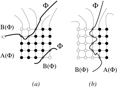
Figure 3: Parts (a) and (b) show a grid of type $A$ and a grid of type $C$, respectively.

Claim 4.2. For any $1\leq i\leq n$,

(i)  if $V_{i}$ is of type A (resp. of type B), then $|C_{i}|\geq w(B_{i})d_{i}$ (resp. $|C_{i}|\geq w(A_{i})d_{i}$);

(ii)  if $V_{i}$ is of type C, then $|C_{i}|\geq{d_{i}\over 6}$.

Proof. In $V_{i}$, every connected component belonging to $A_{i}$ is separated from every connected component belonging to $B_{i}$ by vertices in $C_{i}$. There are $w(A_{i})d_{i}$ (resp. $w(B_{i})d_{i}$) special boundary vertices in $V_{i},$ which belong to $A_{i}$ (resp. $B_{i}$). It can be shown by an easy case analysis that the number of separating points $|C_{i}|\geq\min\{w(A_{i}),w(B_{i})\}d_{i}$, and Claim 4.2 follows; see Fig. 3. $\Box$

Claim 4.3. Let $V=V(G)$. There is a closed curve $\Psi$, not passing through any vertex of $H$, whose interior and exterior are denoted by $A(\Psi)$ and $B(\Psi)$, resp., such that

(i)    $V\cap A(\Psi)=V_{A}$,

(ii)   $V\cap B(\Psi)=V_{B}$,

(iii)  the total number of edges of $G$ intersected by $\Psi$ is at most

$$18\sqrt{{c}(G)+\sum_{i=1}^{n}d_{i}^{2}+n}.$$

Proof. For any $1\leq i\leq m$, we say that

$V_{i}$ is of type 1   if $|C_{i}|\geq d_{i}/6$,

$V_{i}$ is of type 2   if $|C_{i}|<d_{i}/6$.

For every $v\in V_{0}$,

$v$ is of type 1   if $v\in\Phi$,

$v$ is of type 2   if $v\in A(\Phi)\cup B(\Phi)$.

It follows from Claim 4.2 that if a set $V_{i}$ or an isolated vertex $v\in V_{0}$ is of type C, then it is also of type 1.

Next, we modify the curve $\Phi$ in small neighborhoods of the grids $V_{i}$ and of the isolated vertices $v\in V_{0}$ to make sure that the resulting curve $\Psi$ satisfies the conditions in the claim.

Assume for simplicity that $v_{i}\in V_{A}$; the case $v_{i}\in V_{B}$ can be treated analogously. If $v_{i}$ is a vertex of degree at most $1$ and $\Phi$ passes through $v_{i}$, slightly perturb $\Phi$ in a small neighborhood of $v_{i}$ (or slightly shift $v_{i}$) so that after this change $v_{i}$ lies in the interior of $\Phi$. Suppose next that the degree of $v_{i}$ is at least $2$. Let $S_{i}$ and $S^{\prime}_{i}\subset S_{i}$ be two closed squares containing $V_{i}$ in their interiors, and assume that $S_{i}$ (and, hence, $S^{\prime}_{i}$) is only slightly larger than the convex hull of the vertices of $V_{i}$. We distinguish two cases.

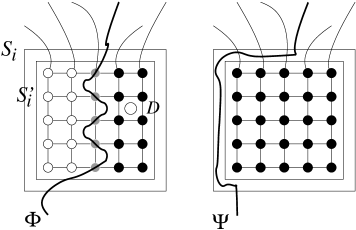
Figure 4: Claim 4.3, Case 1.

Case 1. $V_{i}$ is of type 1. Let $D$ be a small disk in $S^{\prime}_{i}$ that belongs to the interior of $\Phi$ and let $p$ be its center. Let $\tau:S_{i}\rightarrow S_{i}$ be a homeomorphism of $S_{i}$ to itself which keeps the boundary of $S_{i}$ fixed and let $\tau(D)=S^{\prime}_{i}$. Observe that every piece of $\Phi$ within the convex hull of the vertices of $V_{i}$ is mapped into an arc in the very narrow ring $S_{i}\setminus S^{\prime}_{i}$. In particular, if we keep the vertices and the edges of the grid $H[V_{i}]$ (as well as all other parts of the drawing) fixed, after this local modification $\Phi$ will avoid all vertices of $V_{i}$ and it may intersect only those (at most $d_{i}$) edges incident to $V_{i}$ which correspond to original edges of $G$ and end at some special boundary vertex of $V_{i}$. Moreover, after this modification, every vertex of $V_{i}$ will lie in $A(\Phi)$, in the interior of $\Phi$.

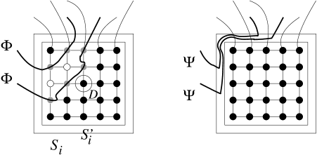
Figure 5: Claim 4.3, Case 2.

Case 2. $V_{i}$ is of type 2. In this case, by Claim 4.2, $V_{i}$ is of type $A$.

Orient $\Phi$ arbitrarily. Let $(p_{1},p_{1}^{\prime}),(p_{2},p_{2}^{\prime}),\ldots$ denote the point pairs at which $\Phi$ enters and leaves the convex hull of $V_{i}$, so that the arc between $p_{j}p^{\prime}_{j}$ lies inside the convex hull of $V_{i}$, for every $j$. Note that both $p_{j}$ and $p^{\prime}_{j}$ are vertices of $V_{i}$. In view of the fact that $|C_{i}|\leq d_{i}/6$, we know that the (graph) distance between $p_{j}$ and $p_{j}^{\prime}$ (in $H[V_{i}]$) is at most $d_{i}/6$. More precisely, for every $j$, the points $p_{j}$ and $p_{j}^{\prime}$ divide the boundary of the convex hull of $V_{i}$ into two arcs. We call the shorter of these arcs the boundary interval defined by $p_{j}$ and $p_{j}^{\prime}$, and denote it by $[p_{j},p_{j}^{\prime}]$. By assumption, the length of $[p_{j},p_{j}^{\prime}]$. the number of edges of $H[V_{i}]$ comprising $[p_{j},p_{j}^{\prime}]$, is at most $d_{i}/6$.

It is not hard to see that the curve $\Phi$ cannot came close to the center $p$ of $V_{i}$ and that $p$ belongs to the interior of $\Phi$. Let $D$ be a small disk centered at $p$. Then $D$ also belongs to the interior of $\Phi$. Let $\tau:S_{i}\rightarrow S_{i}$ be a homeomorphism of $S_{i}$ to itself such that (i) $\tau$ keeps the boundary of $S_{i}$ fixed, (ii) $\tau(D)=S^{\prime}_{i}$, (iii) $\tau(p)=p$, and (iv) for any $q\in S_{i}$, that points $p$, $q$, and $\tau(q)$ are collinear. Observe that every piece $(p_{j},p_{j}^{\prime})$, of $\Phi$ within the convex hull of the vertices of $V_{i}$ is mapped into an arc in the very narrow ring $S_{i}\setminus S^{\prime}_{i}$, along the corresponding boundary interval, $[p_{j},p_{j}^{\prime}]$, defined by $p_{j}$ and $p_{j}^{\prime}$. In particular, if we keep the vertices and edges of the grid $H[V_{i}]$ (as well as all other parts of the drawing) fixed, after this local modification $\Phi$ will avoid all vertices of $V_{i}$ and it may intersect only those (at most $d_{i}/6$) edges incident to $V_{i}$ which correspond to original edges of $G$ and end at some special boundary vertex of $V_{i}$ in a boundary interval. Moreover, now every vertex of $V_{i}$ will lie inside $\Phi$.

Repeat the above local modification for each $V_{i}$ and for each $v\in V_{0}$. The resulting curve, $\Psi$, satisfies conditions (i) and (ii). It remains to show that it also satisfies (iii).

To see this, denote by $E_{X}$ the set of all edges of $H$ adjacent to at least one element of $C_{X}$. For any $1\leq i\leq m$, define $E_{i}\subset E(H)$ as follows. If $V_{i}$ is of type 1, then let all edges of $H$ leaving $V_{i}$ belong to $E_{i}$. If $V_{i}$ is of type 2, then by Claim 4.2, it can be of type A or B, but not C. Let $E_{i}$ consist of all edges leaving $V_{i}$ and crossed by $\Psi$.

For any $1\leq i\leq m$, let $E^{\prime}_{i}$ denote the set of edges of $G$ corresponding to the elements of $E_{i}$ ($0\leq i\leq m$) and let $E^{\prime}_{X}$ denote the set of edges corresponding to the elements of $E_{X}$.

Clearly, we have $|E^{\prime}_{i}|\leq|E_{i}|,$ because distinct edges of $G$ give rise to distinct edges of $H$. Since $V_{A}$ and $V_{B}$ are on different sides of $\Psi$, it crosses all edges between $V_{A}$ and $V_{B}$.

Obviously, $|E^{\prime}_{X}|\leq|E_{X}|\leq 4|C_{X}|$. By Claim 4.2, if $V_{i}$ is of type 1, then $|E^{\prime}_{i}|\leq|E_{i}|=d_{i}\leq 6|C_{i}|$. If $V_{i}$ is of type 2, then $|E^{\prime}_{i}|\leq|E_{i}|=d_{i}\leq|C_{i}|$. Therefore,

$$|E(V_{A},V_{B})|\leq|\cup_{i=0}^{n}E^{\prime}_{i}|\leq\sum_{i=0}^{n}|E_{i}|\leq 6|C|\leq 18\sqrt{{c}(G)+\sum_{i=1}^{n}d_{i}^{2}+n}.$$

This finishes the proof of Claim 4.3. $\Box$

Now we are in a position to complete the proof of Theorem 2. Remove those edges of $G$ that are cut by $\Psi$. Let $G_{A}$ (resp. $G_{B}$) be the subgraph of the resulting graph $G^{\prime}$, induced by $V_{A}$ (resp. $V_{B}$), with the inherited drawing. Suppose that, e.g., $G_{B}$ is not a branching topological graph. Then it has an empty lens, that is, a region bounded by two parallel edges that does not contain any vertex of $V_{B}$. There are two types of empty lenses: bounded and unbounded. We show that there are at most $\sqrt{{c}(G)}$ bounded empty lenses, and at most $\sqrt{{c}(G)}$ unbounded empty lenses in $G_{B}$.

Suppose that $e$ and $e^{\prime}$ are two parallel edges between $v$ and $v^{\prime}$ which enclose a bounded empty lens $L$. Then $v$ and $v^{\prime}$ are in the exterior of $\Psi$, and $\Psi$ does not cross the edges $e$ and $e^{\prime}$. As $G$ was a branching topological multigraph, both $L$ and its complement contain at least one vertex of $G$ in their interiors. Since $L$ is empty in $G_{B}$, it follows that all vertices of $G$ inside $L$ must belong to $V_{A}$, and, hence, must lie in the interior of $\Psi$. Thus, $\Psi$ must lie entirely inside the lens $L$.

Suppose now that $f$ and $f^{\prime}$ are two other parallel edges between two vertices $u$ and $u^{\prime}$, and they determine another bounded empty lens $M$. Arguing as above, we obtain that $\Psi$ must also lie entirely inside $M$. Then $v$ and $v^{\prime}$ are outside of $M$, and $u$ and $u^{\prime}$ are outside of $L$. Therefore, these four edges determine four crossings. Any such crossing can belong to only one pair of bounded empty lenses $\{L,M\}$, we conclude that for the number of bounded empty lenses $k$ in $G_{B}$ we have $4{f\choose 2}\leq c(G)$, therefore, $k\leq\sqrt{{c}(G)}$. Analogously, there are at most $\sqrt{{c}(G)}$ unbounded empty lenses in $G_{B}$.

We can argue in exactly the same way for $G_{A}$. Thus, altogether there are at most $4\sqrt{{c}(G)}$ empty lenses in $G_{A}$ and $G_{B}$. If we delete a boundary edge of each of them, then no empty lens is left.

Thus, by deleting the edges of $G$ crossed by $\Psi$ and then one boundary edge of each empty lens, we obtain a decomposition of $G$ into two branching topological multigraphs, and the number of deleted edges is at most

$$18\sqrt{{c}(G)+\sum_{i=1}^{n}d_{i}^{2}+n}+4\sqrt{{c}(G)}\leq 22\sqrt{{c}(G)+\sum_{i=1}^{n}d_{i}^{2}+n}.$$

This concludes the proof of Theorem 2. $\Box$

Acknowledgement. We are very grateful to Stefan Felsner, Michael Kaufmann, Vincenzo Roselli, Torsten Ueckerdt, and Pavel Valtr for their many valuable comments, suggestions, and for many interesting discussions during the Dagstuhl Seminar ”Beyond-Planar Graphs: Algorithmics and Combinatorics”, November 6-11, 2016,
http://www.dagstuhl.de/en/program/calendar/semhp/?semnr=16452.

References

- [1] M. Ajtai, V. Chvátal, M. N. Newborn, and E. Szemerédi: Crossing-free subgraphs, in: Theory and Practice of Combinatorics, North-Holland Mathematics Studies 60, North-Holland, Amsterdam, 9–12, 1982.
- [2] N. Alon, P. Seymour, and R. Thomas: Planar separators, SIAM J. Discrete Math. 7 (1994), no. 2, 184–193.
- [3] T. L. Dey: Improved bounds for planar -sets and related problems, Discrete & Computational Geometry 19 (1998) (3), 373–382.
- [4] M. R. Garey and D. S. Johnson: Crossing number is NP-complete, SIAM Journal on Algebraic Discrete Methods 4 (1983), no. 3, 312-–316.
- [5] M. Kaufmann, personal communication at the workshop “Beyond-Planar Graphs: Algorithmics and Combinatorics”, Schloss Dagstuhl, Germany, November 6–11, 2016.
- [6] T. Leighton: Complexity Issues in VLSI, Foundations of Computing Series, MIT Press, Cambridge, 1983.
- [7] J. Pach, F. Shahrokhi, and M. Szegedy: Applications of the crossing number, Algorithmica 16 (1996), no. 1, 111–117.
- [8] J. Pach, J. Spencer, and G. Tóth: New bounds for crossing numbers, in Proceedings of the 15th Annual ACM Symposium on Computational Geometry 1999, 124–133. Also in: Discrete & Computational Geometry 24 (2000), 623–644.
- [9] J. Pach and G. Tóth: Thirteen problems on crossing numbers, Geombinatorics 9 (2000), no. 4, 199–207.
- [10] M. Schaefer: Complexity of some geometric and topological problems: Graph Drawing, 17th International Symposium, GS 2009, Chicago, IL, USA, September 2009. Lecture Notes in Computer Science 5849 (2010), Springer-Verlag, 334–344.
- [11] M. Schaefer: The Graph Crossing Number and its Variants: A Survey The Electronic Journal of Combinatorics 1000, Dynamic Survey, DS21, 2013.
- [12] M. Sharir and P. K. Agarwal: Davenport-Schinzel Sequences and Their Geometric Applications, Cambridge University Press, Cambridge, 1995.
- [13] L. A. Székely: Crossing numbers and hard Erdős problems in discrete geometry, Combin. Probab. Comput. 6 (1997), no. 3, 353–358.
- [14] L. A. Székely: A successful concept for measuring non-planarity of graphs: the crossing number. In: 6th International Conference on Graph Theory. Discrete Math. 276 (2004), no. 1–3, 331–-352.
- [15] E. Szemerédi and W. T. Trotter: Extremal problems in discrete geometry, Combinatorica 3 (1983) (3–4), 381–392.