Lorentzian geometry of qubit entanglement

Abstract

We study the relation between qubit entanglement and Lorentzian geometry. In an earlier paper, we had given a recipe for detecting two qubit entanglement. The entanglement criterion is based on Partial Lorentz Transformations (PLT) on individual qubits. The present paper gives the theoretical framework underlying the PLT test. The treatment is based physically, on the causal structure of Minkowski spacetime, and mathematically, on a Lorentzian Singular Value Decomposition. A surprising feature is the natural emergence of “Energy conditions” used in Relativity. All states satisfy a “Dominant Energy Condition” (DEC) and separable states satisfy the Strong Energy Condition(SEC), while entangled states violate the SEC. Apart from testing for entanglement, our approach also enables us to construct a separable form for the density matrix in those cases where it exists. Our approach leads to a simple graphical three dimensional representation of the state space which shows the entangled states within the set of all states.

I I. Introduction

Detecting entanglement is one of the outstanding problems in Quantum Information Theory. In two qubit systems, the Positive Partial Transpose (PPT) criterion Peres (1996); Horodecki et al. (1996); Bengtsson and Zyczkowski (2007) gives a simple, computable criterion for detecting entanglement. The criterion gives a necessary and suficient condition for a state to be separable.

In an earlier paperSamuel et al. (2017), we proposed a new test based on Partial Lorentz Transformation(PLT) of individual qubits. It turns out that like the PPT test, the PLT criterion is necessary and sufficient in the two qubit case. In Samuel et al. (2017), the PLT test was given as a recipe, a form that could be directly used by those who want to apply the test. The purpose of the present paper is to describe the theoretical framework behind the PLT test. In addition to showing why the test works, our Lorentzian approach yields an explicit separable form of the density matrix, when such a form exists. It also permits a complete elucidation of the state space using a Lorentzian version of the Singular Value Decomposition. The PLT test uses ideas borrowed from the space-time physics of Special Relativity.

The paper is organized as follows. In Section II we discuss Partial Lorentz Transformations (PLT). Section III describes the Lorentzian Singular Value Decomposition which provides the theoretical basis for the PLT test. Section IV gives necessary and sufficient conditions on the singular values to define a state and expresses the state in separable form, under certain conditions on the singular values. We also show that these conditions are necessary for separability. We then discuss a simple three dimensional representation of the two-qubit state space in Section V. Section VI deals with non generic states. We finally end the paper with some concluding remarks in Section VII.

We use a Lorentzian metric of signature mostly minus: $g=diag(1,-1,-1,-1)$. Spacetime Lorentz indices $\mu,\nu$ range over $0,1,2,3$, as also do Frame indices $a,b,..$. Both these indices are raised and lowered by the Minkowski metric and we use the Einstein summation convention. All causal (timelike or lightlike 4-vectors) are pointing into the future. Throughout this paper, by “Lorentz group”, we mean its proper, orthochronous subgroup, which preserves time orientation as well as the spatial orientation.

II II. Lorentz Transformations

The states of a qubit can be expressed in space-time form by using $\sigma_{\mu}=(\mathds{1},\sigma_{x},\sigma_{y},\sigma_{z})$, the identity and the Pauli matrices

$$\tau=u^{\mu}\sigma_{\mu}$$ (1)

$u^{\mu}$ is a real future pointing $4$-vector and satisfies

$$u^{\mu}u^{\nu}g_{\mu\nu}>0$$ (2)

for impure states and

$$u^{\mu}u^{\nu}g_{\mu\nu}=0$$ (3)

for pure states. Impure states have time-like $u$ and pure states have lightlike $u$. In both the cases $u^{0}>0$, the 4-vector $u^{\mu}$ is future pointing. If we were to fix the “normalization” by $\textrm{Tr}(\rho)=2$, $u^{0}=1$, the impure states can be represented in the Bloch ball $\vec{u}.\vec{u}<1$ and the pure states on the Bloch sphere $\vec{u}.\vec{u}=1$. The Lorentzian nature of the state space is already evident. Under Lorentz Transformations

$$u^{\leavevmode{\mu}}_{\mathchoice{\makebox[4.21783pt][c]{$\displaystyle$}}{\makebox[4.21783pt][c]{$\textstyle$}}{\makebox[2.95248pt][c]{$\scriptstyle$}}{\makebox[2.10892pt][c]{$\scriptscriptstyle$}}}\mapsto u^{\leavevmode{\prime\mu}}_{\mathchoice{\makebox[6.14282pt][c]{$\displaystyle$}}{\makebox[6.14282pt][c]{$\textstyle$}}{\makebox[4.29997pt][c]{$\scriptstyle$}}{\makebox[3.07141pt][c]{$\scriptscriptstyle$}}}=S^{\leavevmode{\mu}\mathchoice{\makebox[3.45787pt][c]{$\displaystyle$}}{\makebox[3.45787pt][c]{$\textstyle$}}{\makebox[2.42052pt][c]{$\scriptstyle$}}{\makebox[1.72893pt][c]{$\scriptscriptstyle$}}}_{\mathchoice{\makebox[4.21783pt][c]{$\displaystyle$}}{\makebox[4.21783pt][c]{$\textstyle$}}{\makebox[2.95248pt][c]{$\scriptstyle$}}{\makebox[2.10892pt][c]{$\scriptscriptstyle$}}\leavevmode{\nu}}u^{\leavevmode{\nu}}_{\mathchoice{\makebox[3.45787pt][c]{$\displaystyle$}}{\makebox[3.45787pt][c]{$\textstyle$}}{\makebox[2.42052pt][c]{$\scriptstyle$}}{\makebox[1.72893pt][c]{$\scriptscriptstyle$}}}$$

where $S^{\leavevmode{\mu}\mathchoice{\makebox[3.45787pt][c]{$\displaystyle$}}{\makebox[3.45787pt][c]{$\textstyle$}}{\makebox[2.42052pt][c]{$\scriptstyle$}}{\makebox[1.72893pt][c]{$\scriptscriptstyle$}}}_{\mathchoice{\makebox[4.21783pt][c]{$\displaystyle$}}{\makebox[4.21783pt][c]{$\textstyle$}}{\makebox[2.95248pt][c]{$\scriptstyle$}}{\makebox[2.10892pt][c]{$\scriptscriptstyle$}}\leavevmode{\nu}}S^{\leavevmode{\alpha}\mathchoice{\makebox[3.95938pt][c]{$\displaystyle$}}{\makebox[3.95938pt][c]{$\textstyle$}}{\makebox[2.77156pt][c]{$\scriptstyle$}}{\makebox[1.97969pt][c]{$\scriptscriptstyle$}}}_{\mathchoice{\makebox[4.4779pt][c]{$\displaystyle$}}{\makebox[4.4779pt][c]{$\textstyle$}}{\makebox[3.13454pt][c]{$\scriptstyle$}}{\makebox[2.23895pt][c]{$\scriptscriptstyle$}}\leavevmode{\beta}}g^{\mathchoice{\makebox[8.69574pt][c]{$\displaystyle$}}{\makebox[8.69574pt][c]{$\textstyle$}}{\makebox[6.08702pt][c]{$\scriptstyle$}}{\makebox[4.34787pt][c]{$\scriptscriptstyle$}}}_{\leavevmode{\mu\alpha}}=g^{\mathchoice{\makebox[7.41725pt][c]{$\displaystyle$}}{\makebox[7.41725pt][c]{$\textstyle$}}{\makebox[5.19208pt][c]{$\scriptstyle$}}{\makebox[3.70862pt][c]{$\scriptscriptstyle$}}}_{\leavevmode{\nu\beta}}$. The Lorentz Transformation maps states to states. The group action has two orbits: the pure states constitute one orbit and the impure states another.

Partial Lorentz Transformations: Let $\rho$ be a density matrix of a two qubit system. We assume $\rho$ is non negative ($\rho\geq 0$), Hermitian ($\rho^{\dagger}=\rho$). In our treatment, we will not need to normalize $\rho$, but we suppose $\rho$ does not vanish identically. One can expand the density matrix $\rho$ as

$$\rho=\frac{1}{4}A^{\mu\nu}\sigma_{\mu}\otimes\sigma_{\nu}$$ (4)

where $A^{\mu\nu}$ can be calculated from

$$A_{\mu\nu}=\textrm{Tr}(\rho\sigma_{\mu}\otimes\sigma_{\nu}).$$ (5)

Consider doing a Lorentz Transformation on just the first subsystem

$$\sigma^{\mathchoice{\makebox[4.21783pt][c]{$\displaystyle$}}{\makebox[4.21783pt][c]{$\textstyle$}}{\makebox[2.95248pt][c]{$\scriptstyle$}}{\makebox[2.10892pt][c]{$\scriptscriptstyle$}}}_{\leavevmode{\mu}}\mapsto\sigma^{\mathchoice{\makebox[4.21783pt][c]{$\displaystyle$}}{\makebox[4.21783pt][c]{$\textstyle$}}{\makebox[2.95248pt][c]{$\scriptstyle$}}{\makebox[2.10892pt][c]{$\scriptscriptstyle$}}\leavevmode{{}^{\prime}}}_{\leavevmode{\mu}\mathchoice{\makebox[1.07799pt][c]{$\displaystyle$}}{\makebox[1.07799pt][c]{$\textstyle$}}{\makebox[0.76999pt][c]{$\scriptstyle$}}{\makebox[0.76999pt][c]{$\scriptscriptstyle$}}}=\sigma^{\mathchoice{\makebox[4.4779pt][c]{$\displaystyle$}}{\makebox[4.4779pt][c]{$\textstyle$}}{\makebox[3.13454pt][c]{$\scriptstyle$}}{\makebox[2.23895pt][c]{$\scriptscriptstyle$}}}_{\leavevmode{\alpha}}L^{\leavevmode{\alpha}\mathchoice{\makebox[4.21783pt][c]{$\displaystyle$}}{\makebox[4.21783pt][c]{$\textstyle$}}{\makebox[2.95248pt][c]{$\scriptstyle$}}{\makebox[2.10892pt][c]{$\scriptscriptstyle$}}}_{\mathchoice{\makebox[4.4779pt][c]{$\displaystyle$}}{\makebox[4.4779pt][c]{$\textstyle$}}{\makebox[3.13454pt][c]{$\scriptstyle$}}{\makebox[2.23895pt][c]{$\scriptscriptstyle$}}\leavevmode{\mu}}.$$ (6)

This results in a new state $\rho^{\prime}=\frac{1}{4}L^{\leavevmode{\mu}\mathchoice{\makebox[4.4779pt][c]{$\displaystyle$}}{\makebox[4.4779pt][c]{$\textstyle$}}{\makebox[3.13454pt][c]{$\scriptstyle$}}{\makebox[2.23895pt][c]{$\scriptscriptstyle$}}}_{\mathchoice{\makebox[4.21783pt][c]{$\displaystyle$}}{\makebox[4.21783pt][c]{$\textstyle$}}{\makebox[2.95248pt][c]{$\scriptstyle$}}{\makebox[2.10892pt][c]{$\scriptscriptstyle$}}\leavevmode{\alpha}}A^{\leavevmode{\alpha\nu}}_{\mathchoice{\makebox[7.93578pt][c]{$\displaystyle$}}{\makebox[7.93578pt][c]{$\textstyle$}}{\makebox[5.55505pt][c]{$\scriptstyle$}}{\makebox[3.96788pt][c]{$\scriptscriptstyle$}}}\sigma^{\mathchoice{\makebox[4.21783pt][c]{$\displaystyle$}}{\makebox[4.21783pt][c]{$\textstyle$}}{\makebox[2.95248pt][c]{$\scriptstyle$}}{\makebox[2.10892pt][c]{$\scriptscriptstyle$}}}_{\leavevmode{\mu}}\otimes\sigma^{\mathchoice{\makebox[3.45787pt][c]{$\displaystyle$}}{\makebox[3.45787pt][c]{$\textstyle$}}{\makebox[2.42052pt][c]{$\scriptstyle$}}{\makebox[1.72893pt][c]{$\scriptscriptstyle$}}}_{\leavevmode{\nu}}$, so

$$A^{\leavevmode{\prime\mu\nu}}_{\mathchoice{\makebox[9.6007pt][c]{$\displaystyle$}}{\makebox[9.6007pt][c]{$\textstyle$}}{\makebox[6.72049pt][c]{$\scriptstyle$}}{\makebox[4.80034pt][c]{$\scriptscriptstyle$}}}=L^{\leavevmode{\mu}\mathchoice{\makebox[4.4779pt][c]{$\displaystyle$}}{\makebox[4.4779pt][c]{$\textstyle$}}{\makebox[3.13454pt][c]{$\scriptstyle$}}{\makebox[2.23895pt][c]{$\scriptscriptstyle$}}}_{\mathchoice{\makebox[4.21783pt][c]{$\displaystyle$}}{\makebox[4.21783pt][c]{$\textstyle$}}{\makebox[2.95248pt][c]{$\scriptstyle$}}{\makebox[2.10892pt][c]{$\scriptscriptstyle$}}\leavevmode{\alpha}}A^{\leavevmode{\alpha\nu}}_{\mathchoice{\makebox[7.93578pt][c]{$\displaystyle$}}{\makebox[7.93578pt][c]{$\textstyle$}}{\makebox[5.55505pt][c]{$\scriptstyle$}}{\makebox[3.96788pt][c]{$\scriptscriptstyle$}}}.$$

We refer to this as a Partial Lorentz Transformation since it acts only on the first subsystem. Similarly one can perform a Partial Lorentz Transformation on the second subsystem

$$A^{\leavevmode{\prime\prime\mu}\leavevmode{\nu}}_{\mathchoice{\makebox[8.06781pt][c]{$\displaystyle$}}{\makebox[8.06781pt][c]{$\textstyle$}}{\makebox[5.64746pt][c]{$\scriptstyle$}}{\makebox[4.0339pt][c]{$\scriptscriptstyle$}}\mathchoice{\makebox[3.45787pt][c]{$\displaystyle$}}{\makebox[3.45787pt][c]{$\textstyle$}}{\makebox[2.42052pt][c]{$\scriptstyle$}}{\makebox[1.72893pt][c]{$\scriptscriptstyle$}}}=A^{\leavevmode{\mu}\leavevmode{\alpha}}_{\mathchoice{\makebox[4.21783pt][c]{$\displaystyle$}}{\makebox[4.21783pt][c]{$\textstyle$}}{\makebox[2.95248pt][c]{$\scriptstyle$}}{\makebox[2.10892pt][c]{$\scriptscriptstyle$}}\mathchoice{\makebox[4.4779pt][c]{$\displaystyle$}}{\makebox[4.4779pt][c]{$\textstyle$}}{\makebox[3.13454pt][c]{$\scriptstyle$}}{\makebox[2.23895pt][c]{$\scriptscriptstyle$}}}R^{\leavevmode{\nu}\mathchoice{\makebox[4.4779pt][c]{$\displaystyle$}}{\makebox[4.4779pt][c]{$\textstyle$}}{\makebox[3.13454pt][c]{$\scriptstyle$}}{\makebox[2.23895pt][c]{$\scriptscriptstyle$}}}_{\mathchoice{\makebox[3.45787pt][c]{$\displaystyle$}}{\makebox[3.45787pt][c]{$\textstyle$}}{\makebox[2.42052pt][c]{$\scriptstyle$}}{\makebox[1.72893pt][c]{$\scriptscriptstyle$}}\leavevmode{\alpha}}.$$

Partial Lorentz Transformations act on $A$ by left (L) and right (R) actions. It is elementary to check that PLT s are completely positiveBengtsson and Zyczkowski (2007) maps on the state space. They also have the important property that they preserve separability of states. The PLT of a separable state is separable. The PLT of an entangled state is entangled. This is the key property of the Partial Lorentz Transformation group that we exploit here.

III III. Lorentzian Singular Value Decomposition

Let us now consider the action of left and right PLTs on the state space. The space of (unnormalized) density matrices is 16 dimensional. The left and the right PLTs generate orbits which are generically $6+6=12$ dimensional. Thus the 16 dimensional state space splits into a 4 parameter family of 12 dimensional fibers. (There are also isolated points where the isotropy subgroup is larger and the fiber smaller). Each fiber is either entirely separable or entirely entangled. Thus we can reduce the problem to the 4 dimensional space of orbits. In order to characterize the orbits, consider

$$B^{\leavevmode{\mu}\mathchoice{\makebox[3.45787pt][c]{$\displaystyle$}}{\makebox[3.45787pt][c]{$\textstyle$}}{\makebox[2.42052pt][c]{$\scriptstyle$}}{\makebox[1.72893pt][c]{$\scriptscriptstyle$}}}_{\mathchoice{\makebox[4.21783pt][c]{$\displaystyle$}}{\makebox[4.21783pt][c]{$\textstyle$}}{\makebox[2.95248pt][c]{$\scriptstyle$}}{\makebox[2.10892pt][c]{$\scriptscriptstyle$}}\leavevmode{\nu}}=A^{\leavevmode{\mu}\mathchoice{\makebox[4.4779pt][c]{$\displaystyle$}}{\makebox[4.4779pt][c]{$\textstyle$}}{\makebox[3.13454pt][c]{$\scriptstyle$}}{\makebox[2.23895pt][c]{$\scriptscriptstyle$}}}_{\mathchoice{\makebox[4.21783pt][c]{$\displaystyle$}}{\makebox[4.21783pt][c]{$\textstyle$}}{\makebox[2.95248pt][c]{$\scriptstyle$}}{\makebox[2.10892pt][c]{$\scriptscriptstyle$}}\leavevmode{\alpha}}A^{\mathchoice{\makebox[3.45787pt][c]{$\displaystyle$}}{\makebox[3.45787pt][c]{$\textstyle$}}{\makebox[2.42052pt][c]{$\scriptstyle$}}{\makebox[1.72893pt][c]{$\scriptscriptstyle$}}\leavevmode{\alpha}}_{\leavevmode{\nu}\mathchoice{\makebox[4.4779pt][c]{$\displaystyle$}}{\makebox[4.4779pt][c]{$\textstyle$}}{\makebox[3.13454pt][c]{$\scriptstyle$}}{\makebox[2.23895pt][c]{$\scriptscriptstyle$}}}.$$ (7)

B is obviously symmetric $B^{\leavevmode{\mu\nu}}_{\mathchoice{\makebox[7.6757pt][c]{$\displaystyle$}}{\makebox[7.6757pt][c]{$\textstyle$}}{\makebox[5.373pt][c]{$\scriptstyle$}}{\makebox[3.83784pt][c]{$\scriptscriptstyle$}}}=B^{\leavevmode{\nu\mu}}_{\mathchoice{\makebox[7.6757pt][c]{$\displaystyle$}}{\makebox[7.6757pt][c]{$\textstyle$}}{\makebox[5.373pt][c]{$\scriptstyle$}}{\makebox[3.83784pt][c]{$\scriptscriptstyle$}}}$. It is easily checked that $\textrm{Tr}(B^{n})$ is invariant under both left and right PLTs. Generically we would expect the four eigenvalues of $B^{\leavevmode{\mu}\mathchoice{\makebox[3.45787pt][c]{$\displaystyle$}}{\makebox[3.45787pt][c]{$\textstyle$}}{\makebox[2.42052pt][c]{$\scriptstyle$}}{\makebox[1.72893pt][c]{$\scriptscriptstyle$}}}_{\mathchoice{\makebox[4.21783pt][c]{$\displaystyle$}}{\makebox[4.21783pt][c]{$\textstyle$}}{\makebox[2.95248pt][c]{$\scriptstyle$}}{\makebox[2.10892pt][c]{$\scriptscriptstyle$}}\leavevmode{\nu}}$ to characterise the orbits.

Just as we constructed $B$ from a state $A$, we can also similarly define $D$

$$D^{\leavevmode{\mu}\mathchoice{\makebox[3.45787pt][c]{$\displaystyle$}}{\makebox[3.45787pt][c]{$\textstyle$}}{\makebox[2.42052pt][c]{$\scriptstyle$}}{\makebox[1.72893pt][c]{$\scriptscriptstyle$}}}_{\mathchoice{\makebox[4.21783pt][c]{$\displaystyle$}}{\makebox[4.21783pt][c]{$\textstyle$}}{\makebox[2.95248pt][c]{$\scriptstyle$}}{\makebox[2.10892pt][c]{$\scriptscriptstyle$}}\leavevmode{\nu}}=A^{\leavevmode{\alpha}\leavevmode{\mu}}_{\mathchoice{\makebox[4.4779pt][c]{$\displaystyle$}}{\makebox[4.4779pt][c]{$\textstyle$}}{\makebox[3.13454pt][c]{$\scriptstyle$}}{\makebox[2.23895pt][c]{$\scriptscriptstyle$}}\mathchoice{\makebox[4.21783pt][c]{$\displaystyle$}}{\makebox[4.21783pt][c]{$\textstyle$}}{\makebox[2.95248pt][c]{$\scriptstyle$}}{\makebox[2.10892pt][c]{$\scriptscriptstyle$}}}A^{\mathchoice{\makebox[4.4779pt][c]{$\displaystyle$}}{\makebox[4.4779pt][c]{$\textstyle$}}{\makebox[3.13454pt][c]{$\scriptstyle$}}{\makebox[2.23895pt][c]{$\scriptscriptstyle$}}\mathchoice{\makebox[3.45787pt][c]{$\displaystyle$}}{\makebox[3.45787pt][c]{$\textstyle$}}{\makebox[2.42052pt][c]{$\scriptstyle$}}{\makebox[1.72893pt][c]{$\scriptscriptstyle$}}}_{\leavevmode{\alpha}\leavevmode{\nu}}.$$ (8)

$B$ and $D$ have the same four eigenvalues since from the cyclicity of the trace we have $\textrm{Tr}(B^{n})=\textrm{Tr}(D^{n})$ for all integer $n$. These common eigenvalues determine the singular values of $A$.

The relation

$$A^{\mathchoice{\makebox[3.95938pt][c]{$\displaystyle$}}{\makebox[3.95938pt][c]{$\textstyle$}}{\makebox[2.77156pt][c]{$\scriptstyle$}}{\makebox[1.97969pt][c]{$\scriptscriptstyle$}}\leavevmode{\mu}}_{\leavevmode{\beta}\mathchoice{\makebox[4.21783pt][c]{$\displaystyle$}}{\makebox[4.21783pt][c]{$\textstyle$}}{\makebox[2.95248pt][c]{$\scriptstyle$}}{\makebox[2.10892pt][c]{$\scriptscriptstyle$}}}A^{\leavevmode{\beta}\mathchoice{\makebox[4.4779pt][c]{$\displaystyle$}}{\makebox[4.4779pt][c]{$\textstyle$}}{\makebox[3.13454pt][c]{$\scriptstyle$}}{\makebox[2.23895pt][c]{$\scriptscriptstyle$}}}_{\mathchoice{\makebox[3.95938pt][c]{$\displaystyle$}}{\makebox[3.95938pt][c]{$\textstyle$}}{\makebox[2.77156pt][c]{$\scriptstyle$}}{\makebox[1.97969pt][c]{$\scriptscriptstyle$}}\leavevmode{\alpha}}A^{\mathchoice{\makebox[3.45787pt][c]{$\displaystyle$}}{\makebox[3.45787pt][c]{$\textstyle$}}{\makebox[2.42052pt][c]{$\scriptstyle$}}{\makebox[1.72893pt][c]{$\scriptscriptstyle$}}\leavevmode{\alpha}}_{\leavevmode{\nu}\mathchoice{\makebox[4.4779pt][c]{$\displaystyle$}}{\makebox[4.4779pt][c]{$\textstyle$}}{\makebox[3.13454pt][c]{$\scriptstyle$}}{\makebox[2.23895pt][c]{$\scriptscriptstyle$}}}=D^{\leavevmode{\mu}\mathchoice{\makebox[4.4779pt][c]{$\displaystyle$}}{\makebox[4.4779pt][c]{$\textstyle$}}{\makebox[3.13454pt][c]{$\scriptstyle$}}{\makebox[2.23895pt][c]{$\scriptscriptstyle$}}}_{\mathchoice{\makebox[4.21783pt][c]{$\displaystyle$}}{\makebox[4.21783pt][c]{$\textstyle$}}{\makebox[2.95248pt][c]{$\scriptstyle$}}{\makebox[2.10892pt][c]{$\scriptscriptstyle$}}\leavevmode{\alpha}}A^{\mathchoice{\makebox[3.45787pt][c]{$\displaystyle$}}{\makebox[3.45787pt][c]{$\textstyle$}}{\makebox[2.42052pt][c]{$\scriptstyle$}}{\makebox[1.72893pt][c]{$\scriptscriptstyle$}}\leavevmode{\alpha}}_{\leavevmode{\nu}\mathchoice{\makebox[4.4779pt][c]{$\displaystyle$}}{\makebox[4.4779pt][c]{$\textstyle$}}{\makebox[3.13454pt][c]{$\scriptstyle$}}{\makebox[2.23895pt][c]{$\scriptscriptstyle$}}}=A^{\mathchoice{\makebox[3.95938pt][c]{$\displaystyle$}}{\makebox[3.95938pt][c]{$\textstyle$}}{\makebox[2.77156pt][c]{$\scriptstyle$}}{\makebox[1.97969pt][c]{$\scriptscriptstyle$}}\leavevmode{\mu}}_{\leavevmode{\beta}\mathchoice{\makebox[4.21783pt][c]{$\displaystyle$}}{\makebox[4.21783pt][c]{$\textstyle$}}{\makebox[2.95248pt][c]{$\scriptstyle$}}{\makebox[2.10892pt][c]{$\scriptscriptstyle$}}}B^{\leavevmode{\beta}\mathchoice{\makebox[3.45787pt][c]{$\displaystyle$}}{\makebox[3.45787pt][c]{$\textstyle$}}{\makebox[2.42052pt][c]{$\scriptstyle$}}{\makebox[1.72893pt][c]{$\scriptscriptstyle$}}}_{\mathchoice{\makebox[3.95938pt][c]{$\displaystyle$}}{\makebox[3.95938pt][c]{$\textstyle$}}{\makebox[2.77156pt][c]{$\scriptstyle$}}{\makebox[1.97969pt][c]{$\scriptscriptstyle$}}\leavevmode{\nu}}$$ (9)

shows that $A$ is an intertwining operatorDuplij et al. (2004) relating the eigenspaces of $B$ and $D$. The eigenspaces of $B$ and $D$ are then used to bring $A$ to its LSVD form.

Dominant Energy Condition: The non-negativity of $\rho$ implies that $\textrm{Tr}\rho(\tau_{1}\otimes\tau_{2})\geq 0$, where $\tau_{1}=n^{\mu}\sigma_{\mu}$ and $\tau_{2}=m^{\mu}\sigma_{\mu}$ are pure 1-qubit states of two subsystems. We conclude that

$$A^{\mathchoice{\makebox[7.6757pt][c]{$\displaystyle$}}{\makebox[7.6757pt][c]{$\textstyle$}}{\makebox[5.373pt][c]{$\scriptstyle$}}{\makebox[3.83784pt][c]{$\scriptscriptstyle$}}}_{\leavevmode{\mu\nu}}n^{\mu}m^{\nu}\geq 0$$ (10)

for all lightlike $n^{\mu},m^{\nu}$. This implies that the linear transformation $A^{\leavevmode{\mu}\mathchoice{\makebox[3.45787pt][c]{$\displaystyle$}}{\makebox[3.45787pt][c]{$\textstyle$}}{\makebox[2.42052pt][c]{$\scriptstyle$}}{\makebox[1.72893pt][c]{$\scriptscriptstyle$}}}_{\mathchoice{\makebox[4.21783pt][c]{$\displaystyle$}}{\makebox[4.21783pt][c]{$\textstyle$}}{\makebox[2.95248pt][c]{$\scriptstyle$}}{\makebox[2.10892pt][c]{$\scriptscriptstyle$}}\leavevmode{\nu}}$ maps causal vectors to causal vectors (see Fig. 1). More explicitly, $A^{\leavevmode{\mu}\mathchoice{\makebox[3.45787pt][c]{$\displaystyle$}}{\makebox[3.45787pt][c]{$\textstyle$}}{\makebox[2.42052pt][c]{$\scriptstyle$}}{\makebox[1.72893pt][c]{$\scriptscriptstyle$}}}_{\mathchoice{\makebox[4.21783pt][c]{$\displaystyle$}}{\makebox[4.21783pt][c]{$\textstyle$}}{\makebox[2.95248pt][c]{$\scriptstyle$}}{\makebox[2.10892pt][c]{$\scriptscriptstyle$}}\leavevmode{\nu}}n^{\nu}$ is causal if $n^{\nu}$ is. This is also true of the transpose of $A$ ($A^{\mathchoice{\makebox[4.21783pt][c]{$\displaystyle$}}{\makebox[4.21783pt][c]{$\textstyle$}}{\makebox[2.95248pt][c]{$\scriptstyle$}}{\makebox[2.10892pt][c]{$\scriptscriptstyle$}}\leavevmode{\nu}}_{\leavevmode{\mu}\mathchoice{\makebox[3.45787pt][c]{$\displaystyle$}}{\makebox[3.45787pt][c]{$\textstyle$}}{\makebox[2.42052pt][c]{$\scriptstyle$}}{\makebox[1.72893pt][c]{$\scriptscriptstyle$}}}n^{\mu}$ is causal for $n^{\mu}$ causal) and the composite maps $B$ and $D$. This property of mapping the light cone into itself is usually demanded of stress energy tensors in Relativity, where it is called (see Appendix) the Dominant Energy Condition (DEC)Hawking and Ellis (1973).

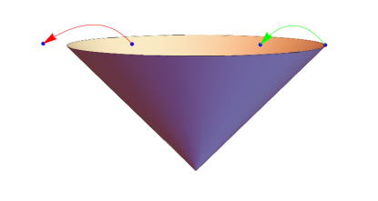
Figure 1: (color online) A representation depicting causal vectors getting mapped to causal vectors (green arrow on the right). The reverse map of a timelike vector going to a space like vector is not allowed (red arrow on the left) by the Dominant Energy Condition.

The dominant energy condition imposes restrictions on the forms that $B$ can take. Hawking and Ellis Hawking and Ellis (1973) give a classification of the canonical forms taken by a symmetric tensor in a Lorentzian space. There are four types, of which only Type-I and Type-II are relevant for us, since the others do not satisfy the DEC. Let $\lambda_{0}$ be the dominant eigenvalue of $B$ (and $D$).

Type-I States: These states are defined by the condition that $B$ admits a timelike eigenvector $e_{0}$ ($B^{\leavevmode{\mu}\mathchoice{\makebox[3.45787pt][c]{$\displaystyle$}}{\makebox[3.45787pt][c]{$\textstyle$}}{\makebox[2.42052pt][c]{$\scriptstyle$}}{\makebox[1.72893pt][c]{$\scriptscriptstyle$}}}_{\mathchoice{\makebox[4.21783pt][c]{$\displaystyle$}}{\makebox[4.21783pt][c]{$\textstyle$}}{\makebox[2.95248pt][c]{$\scriptstyle$}}{\makebox[2.10892pt][c]{$\scriptscriptstyle$}}\leavevmode{\nu}}e_{0}^{\nu}=\lambda_{0}e_{0}^{\mu}$) with $\lambda_{0}>0$. From Eq. (9) it follows that $A^{\mathchoice{\makebox[3.45787pt][c]{$\displaystyle$}}{\makebox[3.45787pt][c]{$\textstyle$}}{\makebox[2.42052pt][c]{$\scriptstyle$}}{\makebox[1.72893pt][c]{$\scriptscriptstyle$}}\leavevmode{\alpha}}_{\leavevmode{\nu}\mathchoice{\makebox[4.4779pt][c]{$\displaystyle$}}{\makebox[4.4779pt][c]{$\textstyle$}}{\makebox[3.13454pt][c]{$\scriptstyle$}}{\makebox[2.23895pt][c]{$\scriptscriptstyle$}}}e_{0}^{\nu}$ is an eigenvector $E_{0}^{\alpha}$ of D with the same eigenvalue $\lambda_{0}$. Computing $E_{0}.E_{0}=\lambda_{0}e_{0}.e_{0}$ we see that $E_{0}$ is timelike, since $e_{0}$ is. Normalising these eigenvectors, we can write (with $\mu_{0}>0$),

$$\mu_{0}E_{0}^{\mu}=A^{\leavevmode{\mu}\mathchoice{\makebox[4.4779pt][c]{$\displaystyle$}}{\makebox[4.4779pt][c]{$\textstyle$}}{\makebox[3.13454pt][c]{$\scriptstyle$}}{\makebox[2.23895pt][c]{$\scriptscriptstyle$}}}_{\mathchoice{\makebox[4.21783pt][c]{$\displaystyle$}}{\makebox[4.21783pt][c]{$\textstyle$}}{\makebox[2.95248pt][c]{$\scriptstyle$}}{\makebox[2.10892pt][c]{$\scriptscriptstyle$}}\leavevmode{\alpha}}e_{0}^{\alpha}$$ (11)

Squaring (11) we find that

$$\lambda_{0}=\mu_{0}^{2}.$$ (12)

Let us define

$$b^{\leavevmode{\mu}\mathchoice{\makebox[3.45787pt][c]{$\displaystyle$}}{\makebox[3.45787pt][c]{$\textstyle$}}{\makebox[2.42052pt][c]{$\scriptstyle$}}{\makebox[1.72893pt][c]{$\scriptscriptstyle$}}}_{\mathchoice{\makebox[4.21783pt][c]{$\displaystyle$}}{\makebox[4.21783pt][c]{$\textstyle$}}{\makebox[2.95248pt][c]{$\scriptstyle$}}{\makebox[2.10892pt][c]{$\scriptscriptstyle$}}\leavevmode{\nu}}=B^{\leavevmode{\mu}\mathchoice{\makebox[3.45787pt][c]{$\displaystyle$}}{\makebox[3.45787pt][c]{$\textstyle$}}{\makebox[2.42052pt][c]{$\scriptstyle$}}{\makebox[1.72893pt][c]{$\scriptscriptstyle$}}}_{\mathchoice{\makebox[4.21783pt][c]{$\displaystyle$}}{\makebox[4.21783pt][c]{$\textstyle$}}{\makebox[2.95248pt][c]{$\scriptstyle$}}{\makebox[2.10892pt][c]{$\scriptscriptstyle$}}\leavevmode{\nu}}-\lambda_{0}e_{0}^{\mu}e^{0}_{\nu}$$

$b$ is symmetric and spatial ($b^{\mathchoice{\makebox[7.6757pt][c]{$\displaystyle$}}{\makebox[7.6757pt][c]{$\textstyle$}}{\makebox[5.373pt][c]{$\scriptstyle$}}{\makebox[3.83784pt][c]{$\scriptscriptstyle$}}}_{\leavevmode{\mu\nu}}=b^{\mathchoice{\makebox[7.6757pt][c]{$\displaystyle$}}{\makebox[7.6757pt][c]{$\textstyle$}}{\makebox[5.373pt][c]{$\scriptstyle$}}{\makebox[3.83784pt][c]{$\scriptscriptstyle$}}}_{\leavevmode{\nu\mu}},\ b^{\mathchoice{\makebox[7.6757pt][c]{$\displaystyle$}}{\makebox[7.6757pt][c]{$\textstyle$}}{\makebox[5.373pt][c]{$\scriptstyle$}}{\makebox[3.83784pt][c]{$\scriptscriptstyle$}}}_{\leavevmode{\mu\nu}}e^{\mathchoice{\makebox[3.5pt][c]{$\displaystyle$}}{\makebox[3.5pt][c]{$\textstyle$}}{\makebox[2.45pt][c]{$\scriptstyle$}}{\makebox[1.75pt][c]{$\scriptscriptstyle$}}\leavevmode{\nu}}_{\leavevmode{0}\mathchoice{\makebox[3.45787pt][c]{$\displaystyle$}}{\makebox[3.45787pt][c]{$\textstyle$}}{\makebox[2.42052pt][c]{$\scriptstyle$}}{\makebox[1.72893pt][c]{$\scriptscriptstyle$}}}=0$) and can therefore be diagonalized by an $SO(3)$ transformation. We thus have a diagonal form for $B$.

The orthonormal frame which diagonalises $B$, ($e_{a}^{\mu}$) gives us a Lorentz tetrad, whose inverse is $e^{a}_{\mu}$. In this frame $B$ has the form:

$$B^{\leavevmode{\mu}\mathchoice{\makebox[3.45787pt][c]{$\displaystyle$}}{\makebox[3.45787pt][c]{$\textstyle$}}{\makebox[2.42052pt][c]{$\scriptstyle$}}{\makebox[1.72893pt][c]{$\scriptscriptstyle$}}}_{\mathchoice{\makebox[4.21783pt][c]{$\displaystyle$}}{\makebox[4.21783pt][c]{$\textstyle$}}{\makebox[2.95248pt][c]{$\scriptstyle$}}{\makebox[2.10892pt][c]{$\scriptscriptstyle$}}\leavevmode{\nu}}=e_{a}^{\mu}B^{\leavevmode{a}\mathchoice{\makebox[3.00417pt][c]{$\displaystyle$}}{\makebox[3.00417pt][c]{$\textstyle$}}{\makebox[2.1029pt][c]{$\scriptstyle$}}{\makebox[1.50208pt][c]{$\scriptscriptstyle$}}}_{\mathchoice{\makebox[3.70012pt][c]{$\displaystyle$}}{\makebox[3.70012pt][c]{$\textstyle$}}{\makebox[2.59009pt][c]{$\scriptstyle$}}{\makebox[1.85005pt][c]{$\scriptscriptstyle$}}\leavevmode{b}}e_{\nu}^{b}.$$ (13)

where $B=diag(\lambda_{0},\lambda_{1},\lambda_{2},\lambda_{3})$. Similarly

$$D^{\leavevmode{\mu}\mathchoice{\makebox[3.45787pt][c]{$\displaystyle$}}{\makebox[3.45787pt][c]{$\textstyle$}}{\makebox[2.42052pt][c]{$\scriptstyle$}}{\makebox[1.72893pt][c]{$\scriptscriptstyle$}}}_{\mathchoice{\makebox[4.21783pt][c]{$\displaystyle$}}{\makebox[4.21783pt][c]{$\textstyle$}}{\makebox[2.95248pt][c]{$\scriptstyle$}}{\makebox[2.10892pt][c]{$\scriptscriptstyle$}}\leavevmode{\nu}}=E_{a}^{\mu}D^{\leavevmode{a}\mathchoice{\makebox[3.00417pt][c]{$\displaystyle$}}{\makebox[3.00417pt][c]{$\textstyle$}}{\makebox[2.1029pt][c]{$\scriptstyle$}}{\makebox[1.50208pt][c]{$\scriptscriptstyle$}}}_{\mathchoice{\makebox[3.70012pt][c]{$\displaystyle$}}{\makebox[3.70012pt][c]{$\textstyle$}}{\makebox[2.59009pt][c]{$\scriptstyle$}}{\makebox[1.85005pt][c]{$\scriptscriptstyle$}}\leavevmode{b}}E_{\nu}^{b}.$$ (14)

$D=diag(\lambda_{0},\lambda_{1},\lambda_{2},\lambda_{3})$. Applying $A$ to $e_{a}^{\nu}$ we have

$$A^{\leavevmode{\mu}\mathchoice{\makebox[3.45787pt][c]{$\displaystyle$}}{\makebox[3.45787pt][c]{$\textstyle$}}{\makebox[2.42052pt][c]{$\scriptstyle$}}{\makebox[1.72893pt][c]{$\scriptscriptstyle$}}}_{\mathchoice{\makebox[4.21783pt][c]{$\displaystyle$}}{\makebox[4.21783pt][c]{$\textstyle$}}{\makebox[2.95248pt][c]{$\scriptstyle$}}{\makebox[2.10892pt][c]{$\scriptscriptstyle$}}\leavevmode{\nu}}e_{a}^{\nu}=\mu_{a}\delta_{a}^{b}E_{b}^{\mu}=T^{\mathchoice{\makebox[3.70012pt][c]{$\displaystyle$}}{\makebox[3.70012pt][c]{$\textstyle$}}{\makebox[2.59009pt][c]{$\scriptstyle$}}{\makebox[1.85005pt][c]{$\scriptscriptstyle$}}\leavevmode{b}}_{\leavevmode{a}\mathchoice{\makebox[3.00417pt][c]{$\displaystyle$}}{\makebox[3.00417pt][c]{$\textstyle$}}{\makebox[2.1029pt][c]{$\scriptstyle$}}{\makebox[1.50208pt][c]{$\scriptscriptstyle$}}}E_{b}^{\mu}$$ (15)

or equivalently

$$A^{\leavevmode{\mu}\mathchoice{\makebox[3.45787pt][c]{$\displaystyle$}}{\makebox[3.45787pt][c]{$\textstyle$}}{\makebox[2.42052pt][c]{$\scriptstyle$}}{\makebox[1.72893pt][c]{$\scriptscriptstyle$}}}_{\mathchoice{\makebox[4.21783pt][c]{$\displaystyle$}}{\makebox[4.21783pt][c]{$\textstyle$}}{\makebox[2.95248pt][c]{$\scriptstyle$}}{\makebox[2.10892pt][c]{$\scriptscriptstyle$}}\leavevmode{\nu}}=E_{b}^{\mu}T^{\leavevmode{b}\mathchoice{\makebox[3.70012pt][c]{$\displaystyle$}}{\makebox[3.70012pt][c]{$\textstyle$}}{\makebox[2.59009pt][c]{$\scriptstyle$}}{\makebox[1.85005pt][c]{$\scriptscriptstyle$}}}_{\mathchoice{\makebox[3.00417pt][c]{$\displaystyle$}}{\makebox[3.00417pt][c]{$\textstyle$}}{\makebox[2.1029pt][c]{$\scriptstyle$}}{\makebox[1.50208pt][c]{$\scriptscriptstyle$}}\leavevmode{a}}e_{\nu}^{a},$$ (16)

where $T^{\leavevmode{a}\mathchoice{\makebox[3.00417pt][c]{$\displaystyle$}}{\makebox[3.00417pt][c]{$\textstyle$}}{\makebox[2.1029pt][c]{$\scriptstyle$}}{\makebox[1.50208pt][c]{$\scriptscriptstyle$}}}_{\mathchoice{\makebox[3.70012pt][c]{$\displaystyle$}}{\makebox[3.70012pt][c]{$\textstyle$}}{\makebox[2.59009pt][c]{$\scriptstyle$}}{\makebox[1.85005pt][c]{$\scriptscriptstyle$}}\leavevmode{b}}$ is diagonal with the form

$$T^{\leavevmode{a}\mathchoice{\makebox[3.00417pt][c]{$\displaystyle$}}{\makebox[3.00417pt][c]{$\textstyle$}}{\makebox[2.1029pt][c]{$\scriptstyle$}}{\makebox[1.50208pt][c]{$\scriptscriptstyle$}}}_{\mathchoice{\makebox[3.70012pt][c]{$\displaystyle$}}{\makebox[3.70012pt][c]{$\textstyle$}}{\makebox[2.59009pt][c]{$\scriptstyle$}}{\makebox[1.85005pt][c]{$\scriptscriptstyle$}}\leavevmode{b}}=\begin{pmatrix}\mu_{0}&0&0&0\\ 0&\mu_{1}&0&0\\ 0&0&\mu_{2}&0\\ 0&0&0&\mu_{3}\end{pmatrix}$$ (17)

The $\mu$ s are the singular values of $A$ and $e^{\mathchoice{\makebox[3.70012pt][c]{$\displaystyle$}}{\makebox[3.70012pt][c]{$\textstyle$}}{\makebox[2.59009pt][c]{$\scriptstyle$}}{\makebox[1.85005pt][c]{$\scriptscriptstyle$}}\leavevmode{\mu}}_{\leavevmode{a}\mathchoice{\makebox[4.21783pt][c]{$\displaystyle$}}{\makebox[4.21783pt][c]{$\textstyle$}}{\makebox[2.95248pt][c]{$\scriptstyle$}}{\makebox[2.10892pt][c]{$\scriptscriptstyle$}}}$ and $E^{\leavevmode{b}\mathchoice{\makebox[3.45787pt][c]{$\displaystyle$}}{\makebox[3.45787pt][c]{$\textstyle$}}{\makebox[2.42052pt][c]{$\scriptstyle$}}{\makebox[1.72893pt][c]{$\scriptscriptstyle$}}}_{\mathchoice{\makebox[3.00417pt][c]{$\displaystyle$}}{\makebox[3.00417pt][c]{$\textstyle$}}{\makebox[2.1029pt][c]{$\scriptstyle$}}{\makebox[1.50208pt][c]{$\scriptscriptstyle$}}\leavevmode{\nu}}$ the left and right Partial Lorentz Transformations that bring A to the LSVD (Lorentzian Singular Value Decomposition) form (17). Since the eigenvalues of $B$ are the squares of the singular values of $A$, it follows that $\lambda$s are positive. At this stage $\mu_{1},\mu_{2},\mu_{3}$ can all have either sign. By Partial Lorentz transformations (e.g by rotation by $\pi$ in the $x-y$ plane) it is possible to reverse the signs of two of $\mu_{1},\mu_{2},\mu_{3}$. By such transformations it is possible to arrange for all of $\mu_{1},\mu_{2},\mu_{3}$ to have the same sign. $\mu_{0}$, of course, is positive (12).

IV IV States and Separability

The DEC is a necessary condition for $\rho$ to be a state (have non negative eigenvalues). From the LSVD form (17) it is easy to write down sufficient conditions on the $\mu$s to ensure that $\rho$ is positive. The diagonal form (17) leads to a state $\rho$

$$\left(\begin{array}[]{cccc}\mu_{0}-\text{$\mu_{3}$}&0&0&\text{$\mu_{2}$}-\text{$\mu_{1}$}\\ 0&\text{$\mu_{3}$}+\mu_{0}&-\text{$\mu_{1}$}-\text{$\mu_{2}$}&0\\ 0&-\text{$\mu_{1}$}-\text{$\mu_{2}$}&\text{$\mu_{3}$}+\mu_{0}&0\\ \text{$\mu_{2}$}-\text{$\mu_{1}$}&0&0&\mu_{0}-\text{$\mu_{3}$}\\ \end{array}\right)$$ (18)

with eigenvalues

$$\mu_{1}-\mu_{2}-\mu_{3} + \mu_{0}$$

$$-\mu_{1}+\mu_{2}-\mu_{3} + \mu_{0}$$

$$-\mu_{1}-\mu_{2}+\mu_{3} + \mu_{0}$$

$$\mu_{1}+\mu_{2}+\mu_{3} + \mu_{0}$$

Requiring that the eigenvalues of $\rho$ are positive gives us the conditions

$$-\mu_{1}+\mu_{2}+\mu_{3} \leq \mu_{0}$$

$$\mu_{1}-\mu_{2}+\mu_{3} \leq \mu_{0}$$

$$\mu_{1}+\mu_{2}-\mu_{3} \leq \mu_{0}$$

$$\mu_{1}+\mu_{2}+\mu_{3} \geq -\mu_{0}$$

The form of $T^{\leavevmode{a}\mathchoice{\makebox[3.00417pt][c]{$\displaystyle$}}{\makebox[3.00417pt][c]{$\textstyle$}}{\makebox[2.1029pt][c]{$\scriptstyle$}}{\makebox[1.50208pt][c]{$\scriptscriptstyle$}}}_{\mathchoice{\makebox[3.70012pt][c]{$\displaystyle$}}{\makebox[3.70012pt][c]{$\textstyle$}}{\makebox[2.59009pt][c]{$\scriptstyle$}}{\makebox[1.85005pt][c]{$\scriptscriptstyle$}}\leavevmode{b}}$ gives us a way to express it in separable form, provided $T^{\leavevmode{a}\mathchoice{\makebox[3.00417pt][c]{$\displaystyle$}}{\makebox[3.00417pt][c]{$\textstyle$}}{\makebox[2.1029pt][c]{$\scriptstyle$}}{\makebox[1.50208pt][c]{$\scriptscriptstyle$}}}_{\mathchoice{\makebox[3.70012pt][c]{$\displaystyle$}}{\makebox[3.70012pt][c]{$\textstyle$}}{\makebox[2.59009pt][c]{$\scriptstyle$}}{\makebox[1.85005pt][c]{$\scriptscriptstyle$}}\leavevmode{b}}$ (See also the appendix below) satisfies the strong energy condition Hawking and Ellis (1973):

$$\mu_{1}+\mu_{2}+\mu_{3}\leq\mu_{0}.$$

Let us define an orthonormal frame $T^{a},X^{a},Y^{a},Z^{a}$ in which $T^{\leavevmode{a}\mathchoice{\makebox[3.00417pt][c]{$\displaystyle$}}{\makebox[3.00417pt][c]{$\textstyle$}}{\makebox[2.1029pt][c]{$\scriptstyle$}}{\makebox[1.50208pt][c]{$\scriptscriptstyle$}}}_{\mathchoice{\makebox[3.70012pt][c]{$\displaystyle$}}{\makebox[3.70012pt][c]{$\textstyle$}}{\makebox[2.59009pt][c]{$\scriptstyle$}}{\makebox[1.85005pt][c]{$\scriptscriptstyle$}}\leavevmode{b}}$ is diagonal. Suppose first that $\mu_{1},\mu_{2},\mu_{3}$ are all non negative.

$$T^{\leavevmode{a}\mathchoice{\makebox[3.00417pt][c]{$\displaystyle$}}{\makebox[3.00417pt][c]{$\textstyle$}}{\makebox[2.1029pt][c]{$\scriptstyle$}}{\makebox[1.50208pt][c]{$\scriptscriptstyle$}}}_{\mathchoice{\makebox[3.70012pt][c]{$\displaystyle$}}{\makebox[3.70012pt][c]{$\textstyle$}}{\makebox[2.59009pt][c]{$\scriptstyle$}}{\makebox[1.85005pt][c]{$\scriptscriptstyle$}}\leavevmode{b}}=\mu_{1}X^{a}X_{b}+\mu_{2}Y^{a}Y_{b}+\mu_{3}Z^{a}Z_{b}+\mu_{0}T^{a}T_{b}$$ (21)

Let us also define lightlike vectors $X_{\pm}=(T\pm X)/\sqrt{2}$ and similarly $Y_{\pm}$ and $Z_{\pm}$. From the identity

$$X_{+}^{a}X_{+b}+X_{-}^{a}X_{-b}=X^{a}X_{b}+T^{a}T_{b}$$ (22)

we can write $T^{\leavevmode{a}\mathchoice{\makebox[3.00417pt][c]{$\displaystyle$}}{\makebox[3.00417pt][c]{$\textstyle$}}{\makebox[2.1029pt][c]{$\scriptstyle$}}{\makebox[1.50208pt][c]{$\scriptscriptstyle$}}}_{\mathchoice{\makebox[3.70012pt][c]{$\displaystyle$}}{\makebox[3.70012pt][c]{$\textstyle$}}{\makebox[2.59009pt][c]{$\scriptstyle$}}{\makebox[1.85005pt][c]{$\scriptscriptstyle$}}\leavevmode{b}}$ as

$$T^{\leavevmode{a}\mathchoice{\makebox[3.00417pt][c]{$\displaystyle$}}{\makebox[3.00417pt][c]{$\textstyle$}}{\makebox[2.1029pt][c]{$\scriptstyle$}}{\makebox[1.50208pt][c]{$\scriptscriptstyle$}}}_{\mathchoice{\makebox[3.70012pt][c]{$\displaystyle$}}{\makebox[3.70012pt][c]{$\textstyle$}}{\makebox[2.59009pt][c]{$\scriptstyle$}}{\makebox[1.85005pt][c]{$\scriptscriptstyle$}}\leavevmode{b}}= \mu_{1}(X_{+}^{a}X_{+b}+X_{-}^{a}X_{-b})$$ (23)

$$+ \mu_{2}(Y_{+}^{a}Y_{+b}+Y_{-}^{a}Y_{-b})$$

$$+ \mu_{3}(Z_{+}^{a}Z_{+b}+Z_{-}^{a}Z_{-b})$$

$$+ (\mu_{0}-\mu_{1}-\mu_{2}-\mu_{3})T^{a}T_{b}$$

$T$ is explicitly in separable form provided

$$\mu_{0}\geq\mu_{1}+\mu_{2}+\mu_{3},$$

i.e. the Strong Energy Condition(SEC) is satisfied.

If $\mu_{1},\mu_{2},\mu_{3}$ are all non positive, they automatically satisfy (LABEL:stateconditions) $|\mu_{1}|+|\mu_{2}|+|\mu_{3}|\leq\mu_{0}$. The identity

$$X_{+}^{a}X_{-b}+X_{-}^{a}X_{+b}=-X^{a}X_{b}+T^{a}T_{b}$$ (24)

gives us

$$T^{\leavevmode{a}\mathchoice{\makebox[3.00417pt][c]{$\displaystyle$}}{\makebox[3.00417pt][c]{$\textstyle$}}{\makebox[2.1029pt][c]{$\scriptstyle$}}{\makebox[1.50208pt][c]{$\scriptscriptstyle$}}}_{\mathchoice{\makebox[3.70012pt][c]{$\displaystyle$}}{\makebox[3.70012pt][c]{$\textstyle$}}{\makebox[2.59009pt][c]{$\scriptstyle$}}{\makebox[1.85005pt][c]{$\scriptscriptstyle$}}\leavevmode{b}}= |\mu_{1}|(X_{+}^{a}X_{-b}+X_{-}^{a}X_{+b})$$ (25)

$$+ |\mu_{2}|(Y_{+}^{a}Y_{-b}+Y_{-}^{a}Y_{+b})$$

$$+ |\mu_{3}|(Z_{+}^{a}Z_{-b}+Z_{-}^{a}Z_{+b})$$

$$+ (\mu_{0}-|\mu_{1}|-|\mu_{2}|-|\mu_{3}|)T^{a}T_{b},$$

which is in separable form.

Conversely, if $A$ represents a separable state, we can write

$$A_{\mu\nu}=\sum_{i}w_{i}\ n_{\mu}^{i}m_{\nu}^{i}$$

where $w_{i}>0$ are positive weights and $n^{i}$ and $m^{i}$ are future pointing causal vectors. Without loss of generality we can suppose $n,m$ to be lightlike (since time-like vectors are convex combinations of lightlike ones) and further absorb $w_{i}$ into the vectors $n,m$. Computing

$$A_{xx}+A_{yy}+A_{zz} = \sum_{i}\vec{n_{i}}.\vec{m_{i}}\ \leq\sum_{i}|n_{i}||m_{i}|$$ (26)

$$= \sum_{i}n_{i0}m_{i0}$$

$$= A_{00}$$

Applying this argument to the LSVD diagonal form $T$, we see that separable states satisfy the SEC. Thus we have shown that the SEC is necessary and sufficient for separability. If the SEC is satisfied we find an explicit decomposition of $T^{\leavevmode{a}\mathchoice{\makebox[3.00417pt][c]{$\displaystyle$}}{\makebox[3.00417pt][c]{$\textstyle$}}{\makebox[2.1029pt][c]{$\scriptstyle$}}{\makebox[1.50208pt][c]{$\scriptscriptstyle$}}}_{\mathchoice{\makebox[3.70012pt][c]{$\displaystyle$}}{\makebox[3.70012pt][c]{$\textstyle$}}{\makebox[2.59009pt][c]{$\scriptstyle$}}{\makebox[1.85005pt][c]{$\scriptscriptstyle$}}\leavevmode{b}}$ (and therefore of $A$) into separable form.

V V. Three dimensional representation of the two-qubit state space

As we discussed earlier, the 16 dimensional space of un-normalized density matrices undergoes a reduction to a 4 parameter family of twelve dimensional fibers under the action of left and right Partial Lorentz Transformations. In fact, the 4 parameter $(\mu_{0},\mu_{1},\mu_{2},\mu_{3})$ representation can be further reduced to a 3 parameter representation since only the ratios are relevant. Since we have assumed $\lambda_{0}\neq 0$ we have $\mu_{0}\neq 0$. By scaling let us set $\mu_{0}=1$ and plot a simple three dimensional representation of the state space. From the DEC, it follows that $0\leq|\mu_{\hat{a}}|\leq 1,{\hat{a}}=1,2,3$, so the states lie within the cube of side $2$ whose body diagonal connects ${\bf{\tilde{P}}}=\{-1,-1,-1\}$ to ${\bf{P}}=\{1,1,1\}$.

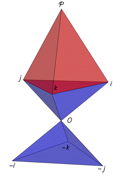
Figure 2: (color online) A three dimensional representation of the state space of $\mu_{1},\mu_{2},\mu_{3}$ for Type-I states. The red tetrahedron (${\bf\{P,i,j,k}\}$) represents the set of entangled states and the blue tetrahedra (${\bf\{O,i,j,k\}}$ and ${\bf\{O,-i,-j,-k\}}$), the set of separable states. The boundary between these two sets is defined by a plane passing through the tips of the unit vectors ${\bf i,j,k}$.

As mentioned earlier, we can suppose that $\mu_{1},\mu_{2},\mu_{3}$ have the same sign. Instead of the eight octants spanned by the cube above, we need only restrict ourselves to two of the eight octants: the positive octant and the negative octant. This results in the figure shown in Fig. 2.

The region shaded blue is the set of separable states. All states in the negative octant are separable and form the convex hull $S^{-}=H(\bf{O},-\bf{i},-\bf{j},-\bf{k})$ of the origin $\bf{O}$ and the tips of the unit vectors $-\bf{i},-\bf{j},-\bf{k}$. The plane passing through $-\bf{i},-\bf{j},-\bf{k}$ divides $\mu$s satisfying the state conditions(LABEL:stateconditions) from those that don’t. In the positive octant, the separable states form the convex hull $S^{+}=H(\bf{O},\bf{i},\bf{j},\bf{k})$ of the origin $\bf{O}$ and the tips of the unit vectors $\bf{i},\bf{j},\bf{k}$. The plane passing through $\bf{i},\bf{j},\bf{k}$ divides the separable states from the entangled states. All states “above” this plane (Fig. 2) are entangled and shown in red.

Note also that under inversion, (reversing the sign of all of $\mu_{1},\mu_{2},\mu_{3}$), the separable states $S^{+}$ and $S^{-}$ exchange places, but the entangled states are mapped to regions outside the state space. In fact, inversion ${\cal I}$ in the $\vec{\mu}$ space is identical to the partial transpose (and to the partial inversion). As expected from the PPT test, the entangled states (in red in Fig. 2) are mapped outside the state space by the partial transpose operation.

Finally we remark that the states on the boundary of $S^{+}$ and $S^{-}$, where one or more $\mu$ s vanishes have to be identified with their images under inversion. With this identification, Fig. 2 gives a complete elucidation of the generic state space. Each point in the state space of Fig. 2 represents an equivalence class of states, all of which are related by partial Lorentz transformations.

The generic state space includes most of the states of the two qubit system, including all strictly positive density matrices. The non generic states are characterised by the absence of a timelike eigenvector for $B$ ($D$). We deal with these in the next section titled exceptional statesAvron and Kenneth (2009).

VI VI Exceptional States

There are some states which do not admit a timelike eigenvector for $B$ ($D$). For this to happen, the dominant eigenvalue $\lambda_{0}$ has to be degenerate.

Type-II States:
These states are characterised by the fact that $B$ ($D$) has a repeated lightlike eigenvector with positive eigenvalue. The dominant eigenvector can be chosen to be $=X_{+}$. For Type-II states, the LSVD matrix $T^{\leavevmode{a}\mathchoice{\makebox[3.00417pt][c]{$\displaystyle$}}{\makebox[3.00417pt][c]{$\textstyle$}}{\makebox[2.1029pt][c]{$\scriptstyle$}}{\makebox[1.50208pt][c]{$\scriptscriptstyle$}}}_{\mathchoice{\makebox[3.70012pt][c]{$\displaystyle$}}{\makebox[3.70012pt][c]{$\textstyle$}}{\makebox[2.59009pt][c]{$\scriptstyle$}}{\makebox[1.85005pt][c]{$\scriptscriptstyle$}}\leavevmode{b}}$ is not diagonal but only in Jordan form. The basis which achieves this form is not a standard Lorentz frame $\{T,X,Y,Z\}$ but a null frame $\{X_{+},X_{-},Y,Z\}$. The Jordan form is

$$T^{\leavevmode{a}\mathchoice{\makebox[3.00417pt][c]{$\displaystyle$}}{\makebox[3.00417pt][c]{$\textstyle$}}{\makebox[2.1029pt][c]{$\scriptstyle$}}{\makebox[1.50208pt][c]{$\scriptscriptstyle$}}}_{\mathchoice{\makebox[3.70012pt][c]{$\displaystyle$}}{\makebox[3.70012pt][c]{$\textstyle$}}{\makebox[2.59009pt][c]{$\scriptstyle$}}{\makebox[1.85005pt][c]{$\scriptscriptstyle$}}\leavevmode{b}}=\begin{pmatrix}\mu_{0}&0&0&0\\ x&\mu_{0}&0&0\\ 0&0&\mu_{2}&0\\ 0&0&0&\mu_{3}\end{pmatrix}$$ (27)

where $x>0$. (DEC guarantees $x\geq 0$, but if $x$ vanishes, $A$ is of Type-I, since $B$ has two distinct lightlike eigenvectors $X_{+},X_{-}$.) We have arbitrarily selected $\mu_{1}$ degenerate with $\mu_{0}$. Since $\mu_{1}=\mu_{0}$ is positive, we can arrange for $\mu_{2},\mu_{3}$ also to be positive and we have

$$T^{\leavevmode{a}\mathchoice{\makebox[3.00417pt][c]{$\displaystyle$}}{\makebox[3.00417pt][c]{$\textstyle$}}{\makebox[2.1029pt][c]{$\scriptstyle$}}{\makebox[1.50208pt][c]{$\scriptscriptstyle$}}}_{\mathchoice{\makebox[3.70012pt][c]{$\displaystyle$}}{\makebox[3.70012pt][c]{$\textstyle$}}{\makebox[2.59009pt][c]{$\scriptstyle$}}{\makebox[1.85005pt][c]{$\scriptscriptstyle$}}\leavevmode{b}}= \mu_{0}(X_{-}^{a}X_{+b}+X_{+}^{a}X_{-b})$$ (28)

$$+ \mu_{2}(Y_{+}^{a}Y_{+b}+Y_{-}^{a}Y_{-b})$$

$$+ \mu_{3}(Z_{+}^{a}Z_{+b}+Z_{-}^{a}Z_{-b})$$

$$+ xX_{+}^{a}X_{+b}$$

The condition that $A$ is defined from a state (Eq. (LABEL:stateconditions)) requires $\mu_{2}=\mu_{3}$. From the argument at the end of section IV, we see that these states are entangled if $\mu_{2}=\mu_{3}>0$.

If $\mu_{2}=\mu_{3}=0$, then

$$T^{\leavevmode{a}\mathchoice{\makebox[3.00417pt][c]{$\displaystyle$}}{\makebox[3.00417pt][c]{$\textstyle$}}{\makebox[2.1029pt][c]{$\scriptstyle$}}{\makebox[1.50208pt][c]{$\scriptscriptstyle$}}}_{\mathchoice{\makebox[3.70012pt][c]{$\displaystyle$}}{\makebox[3.70012pt][c]{$\textstyle$}}{\makebox[2.59009pt][c]{$\scriptstyle$}}{\makebox[1.85005pt][c]{$\scriptscriptstyle$}}\leavevmode{b}}= \mu_{0}(X_{-}^{a}X_{+b}+X_{+}^{a}X_{-b})+xX_{+}^{a}X_{+b}.$$

These states are clearly in separable form. The Type-II states are shown in Fig. 3. The blue dots represent the separable states and the red lines the entangled ones. By switching the roles of $B$ and $D$, we also have states where the Jordan form is the transpose of (27).

Type-II0 States:
Finally, we address the possibility that the dominant eigenvalue $\lambda_{0}$ vanishes. As described in the appendix, these states come in three families ($t$ is a timelike vector and $x$ is positive):

1. Type-II0a: $A^{\leavevmode{\mu}\mathchoice{\makebox[3.45787pt][c]{$\displaystyle$}}{\makebox[3.45787pt][c]{$\textstyle$}}{\makebox[2.42052pt][c]{$\scriptstyle$}}{\makebox[1.72893pt][c]{$\scriptscriptstyle$}}}_{\mathchoice{\makebox[4.21783pt][c]{$\displaystyle$}}{\makebox[4.21783pt][c]{$\textstyle$}}{\makebox[2.95248pt][c]{$\scriptstyle$}}{\makebox[2.10892pt][c]{$\scriptscriptstyle$}}\leavevmode{\nu}}=xt^{\leavevmode{\mu}}_{\mathchoice{\makebox[4.21783pt][c]{$\displaystyle$}}{\makebox[4.21783pt][c]{$\textstyle$}}{\makebox[2.95248pt][c]{$\scriptstyle$}}{\makebox[2.10892pt][c]{$\scriptscriptstyle$}}}l^{\mathchoice{\makebox[3.45787pt][c]{$\displaystyle$}}{\makebox[3.45787pt][c]{$\textstyle$}}{\makebox[2.42052pt][c]{$\scriptstyle$}}{\makebox[1.72893pt][c]{$\scriptscriptstyle$}}}_{\leavevmode{\nu}}$. $B$ vanishes identically.

2. Type-II0b: $A^{\leavevmode{\mu}\mathchoice{\makebox[3.45787pt][c]{$\displaystyle$}}{\makebox[3.45787pt][c]{$\textstyle$}}{\makebox[2.42052pt][c]{$\scriptstyle$}}{\makebox[1.72893pt][c]{$\scriptscriptstyle$}}}_{\mathchoice{\makebox[4.21783pt][c]{$\displaystyle$}}{\makebox[4.21783pt][c]{$\textstyle$}}{\makebox[2.95248pt][c]{$\scriptstyle$}}{\makebox[2.10892pt][c]{$\scriptscriptstyle$}}\leavevmode{\nu}}=xl^{\leavevmode{\mu}}_{\mathchoice{\makebox[4.21783pt][c]{$\displaystyle$}}{\makebox[4.21783pt][c]{$\textstyle$}}{\makebox[2.95248pt][c]{$\scriptstyle$}}{\makebox[2.10892pt][c]{$\scriptscriptstyle$}}}t^{\mathchoice{\makebox[3.45787pt][c]{$\displaystyle$}}{\makebox[3.45787pt][c]{$\textstyle$}}{\makebox[2.42052pt][c]{$\scriptstyle$}}{\makebox[1.72893pt][c]{$\scriptscriptstyle$}}}_{\leavevmode{\nu}}$. $D$ vanishes identically.

3. Type-II0c: $A^{\leavevmode{\mu}\mathchoice{\makebox[3.45787pt][c]{$\displaystyle$}}{\makebox[3.45787pt][c]{$\textstyle$}}{\makebox[2.42052pt][c]{$\scriptstyle$}}{\makebox[1.72893pt][c]{$\scriptscriptstyle$}}}_{\mathchoice{\makebox[4.21783pt][c]{$\displaystyle$}}{\makebox[4.21783pt][c]{$\textstyle$}}{\makebox[2.95248pt][c]{$\scriptstyle$}}{\makebox[2.10892pt][c]{$\scriptscriptstyle$}}\leavevmode{\nu}}=xl^{\mathchoice{\makebox[3.5pt][c]{$\displaystyle$}}{\makebox[3.5pt][c]{$\textstyle$}}{\makebox[2.45pt][c]{$\scriptstyle$}}{\makebox[1.75pt][c]{$\scriptscriptstyle$}}\leavevmode{\mu}}_{\leavevmode{1}\mathchoice{\makebox[4.21783pt][c]{$\displaystyle$}}{\makebox[4.21783pt][c]{$\textstyle$}}{\makebox[2.95248pt][c]{$\scriptstyle$}}{\makebox[2.10892pt][c]{$\scriptscriptstyle$}}}l^{\mathchoice{\makebox[3.5pt][c]{$\displaystyle$}}{\makebox[3.5pt][c]{$\textstyle$}}{\makebox[2.45pt][c]{$\scriptstyle$}}{\makebox[1.75pt][c]{$\scriptscriptstyle$}}\mathchoice{\makebox[3.45787pt][c]{$\displaystyle$}}{\makebox[3.45787pt][c]{$\textstyle$}}{\makebox[2.42052pt][c]{$\scriptstyle$}}{\makebox[1.72893pt][c]{$\scriptscriptstyle$}}}_{\leavevmode{2}\leavevmode{\nu}}$. Both $B$ and $D$ vanish.

These states are separable and because they have vanishing $\mu_{0}$, do not find a place in either Fig.2 or Fig.3. The form of the stress tensor for Type-II0c is $T^{\leavevmode{a}\mathchoice{\makebox[3.00417pt][c]{$\displaystyle$}}{\makebox[3.00417pt][c]{$\textstyle$}}{\makebox[2.1029pt][c]{$\scriptstyle$}}{\makebox[1.50208pt][c]{$\scriptscriptstyle$}}}_{\mathchoice{\makebox[3.70012pt][c]{$\displaystyle$}}{\makebox[3.70012pt][c]{$\textstyle$}}{\makebox[2.59009pt][c]{$\scriptstyle$}}{\makebox[1.85005pt][c]{$\scriptscriptstyle$}}\leavevmode{b}}=xX^{\mathchoice{\makebox[5.44446pt][c]{$\displaystyle$}}{\makebox[5.44446pt][c]{$\textstyle$}}{\makebox[3.81111pt][c]{$\scriptstyle$}}{\makebox[2.72223pt][c]{$\scriptscriptstyle$}}\leavevmode{a}}_{\leavevmode{+}\mathchoice{\makebox[3.70012pt][c]{$\displaystyle$}}{\makebox[3.70012pt][c]{$\textstyle$}}{\makebox[2.59009pt][c]{$\scriptstyle$}}{\makebox[1.85005pt][c]{$\scriptscriptstyle$}}}X^{\mathchoice{\makebox[10.00417pt][c]{$\displaystyle$}}{\makebox[10.00417pt][c]{$\textstyle$}}{\makebox[5.91402pt][c]{$\scriptstyle$}}{\makebox[4.2243pt][c]{$\scriptscriptstyle$}}}_{\leavevmode{+b}}$. Such a form for the stress tensor appears in Relativity where it is known as a null fluid or null dustHawking and Ellis (1973). It represents radiation which is all travelling in the same direction.

To summarise our classification (which is explained in more detail in the appendix),

1. Type-I: $\lambda_{0}>0$ and $B$ (and $D$) admit a timelike eigenvector.

2. Type-II: $\lambda_{0}>0$ and $B$ (and $D$) has a repeated lightlike eigenvector.

3. Type-II0: $\lambda_{0}=0$. $B$ or $D$ (or both) vanish.

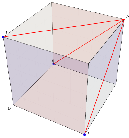
Figure 3: (color online) A three dimensional representation of the state space for Type-II states.The three blue dots at $\{{\bf i,j,k}\}$ represent separable states and the three red lines $\{{\bf i,P}\}$, $\{{\bf j,P}\}$, $\{{\bf k,P}\}$ represent entangled states.

VII VII. Conclusion

We have presented a necessary and sufficient criterion to detect two qubit entanglement. In addition our approach reveals a separable form of the density matrix if it exists. Our approach is based on Lorentzian geometry, in particular a Lorentzian Singular Value Decomposition. The LSVD has also been described by Avron et al Avron and Kenneth (2009). They also notice the relevance of the Dominant Energy Condition that all states must satisfy and go on to give a three dimensional graphical representation of the state space. However, Avron et al Avron and Kenneth (2009) do not propose an entanglement test, as we have done. Neither do they comment on the relevance of the strong energy condition to entanglement. Our graphical representation, though related to Avron and Kenneth (2009), is simpler, because we reduce the picture from eight octants to two. There has also been work Rudolph (2003) which proposes an entanglement test based on a standard Singular Value Decomposition. However, this test only works on a restricted class of states: the reduced density matrices of each subsystem have to be maximally disordered. We go beyond earlier work in providing an explicit construction of a separable state for the density matrix in those cases where it exists.

Our focus in this paper is entirely on quantum entanglement. There are other quantum correlations like discord described for example in Ali et al. (2010), which are not considered here. Ref.Ali et al. (2010) studies the so-called X states, which have nonzero entries on the diagonal and the anti-diagonal. The focus of Ref.Ali et al. (2010) is the study of quantum discord for two qubit X states, with a view to understanding the relation between quantum discord, classical correlations and entanglement. They observe that these are independent measures of correlation.

Ref. Sabapathy and Simon (2013) also addresses X states and quantum discord. Just as we do here, Ref. Sabapathy and Simon (2013) also makes use of Lorentzian structures. However, the local operations considered are local unitary transformations (six parameters in all) and the canonical forms used are X states, which are characterised by essentially five parameters. As a result the total dimension of the state space explored is generically eleven, which falls short of the dimension of fifteen, for normalised states. In contrast, our use of local (or partial) Lorentz transformations provides twelve parameters, which along with the four eigenvalues of the canonical diagonal form provides a complete characterisation of the sixteen dimensional unnormalised state space. It is interesting to note that our Eq. (18) represents an X state, but the number of parameters appearing is only four. In our treatment, not all X states are required to produce the general state by local Lorentz transformations.

There appears to be a rich Lorentzian structure hidden within the theory of quantum entanglement. The relation is probably best appreciated using spinors, which have been studied by relativists like Penrose, Newman etcPenrose and Rindler (1984). In this exposition, we have deliberately avoided the use of spinor language since this is not widely used in the general physics community. The key property of Partial Lorentz Transformations used here is that they map states to states, separable states to separable states and entangled states to entangled states. This allows us to decompose the total set of states into equivalence classes. Any two elements from the same equivalence class are related by Partial Lorentz Transformations and are either both separable or both entangled. To decide whether a particular equivalence class is entangled or separable, we can choose any element from the class. By choosing the canonical form given by the LSVD decomposition, we are able to easily determine if the class is separable or entangled.

Although the test proposed in Samuel et al. (2017) relies only on the eigenvalues of $B$ ($D$), it is important to realise that the state depends both on the eigenvalues and the eigenvectors of $B$ ($D$). While a knowledge of the eigenvalues is enough to determine if a state is separable, one needs also the eigenvectors to explicitly write out the separable form.

By setting quantum states in correspondence with tensors in Minkowski space, we were naturally led to a formalism combining Quantum Information Theory with Relativity. While the analogy at this level is a purely formal one, it may contain the seeds of some future amalgamation of Relativity with Quantum Information Theory. For instance one can consider physical realisations of PLT s by forming two qubits in an entangled state, separating the qubits and acclerating one of them adiabatically to a new Lorentz frame. One would expect the states to transform according to the formulae of this paper.

How does this theory work in higher dimensional quantum systems? It would appear that one has to find a maximal group of transformations which takes states to states and separable states to separable states. These would be the appropriate generalisation of PLT s to the higher dimensional case. Once such a group of entanglement preserving transformations is identified the dimensionality of the problem can be drastically reduced. We hope to interest the quantum information community in this new approach to the problem of detecting quantum entanglement.

VIII Acknowledgements

We thank Anirudh Reddy and Rafael Sorkin for discussions.

IX Appendix A: Energy Conditions

In this appendix we discuss the energy conditions that come into play in our analysis. Given a stress energy tensor $T_{ab}$ one requires it to satisfy some “reasonable” positivity conditions. If $T^{\leavevmode{a}\mathchoice{\makebox[3.00417pt][c]{$\displaystyle$}}{\makebox[3.00417pt][c]{$\textstyle$}}{\makebox[2.1029pt][c]{$\scriptstyle$}}{\makebox[1.50208pt][c]{$\scriptscriptstyle$}}}_{\mathchoice{\makebox[3.70012pt][c]{$\displaystyle$}}{\makebox[3.70012pt][c]{$\textstyle$}}{\makebox[2.59009pt][c]{$\scriptstyle$}}{\makebox[1.85005pt][c]{$\scriptscriptstyle$}}\leavevmode{b}}$ has a timelike eigenvector, it can be diagonalised (Hawking and Ellis (1973)) and brought to the form $T^{\leavevmode{a}\mathchoice{\makebox[3.00417pt][c]{$\displaystyle$}}{\makebox[3.00417pt][c]{$\textstyle$}}{\makebox[2.1029pt][c]{$\scriptstyle$}}{\makebox[1.50208pt][c]{$\scriptscriptstyle$}}}_{\mathchoice{\makebox[3.70012pt][c]{$\displaystyle$}}{\makebox[3.70012pt][c]{$\textstyle$}}{\makebox[2.59009pt][c]{$\scriptstyle$}}{\makebox[1.85005pt][c]{$\scriptscriptstyle$}}\leavevmode{b}}=diag(\epsilon,-p_{1},-p_{2},-p_{3})=diag(\mu_{0},\mu_{1},\mu_{2},\mu_{3})$, where $\epsilon$ is the energy density of matter and $p_{1},p_{2},p_{3}$ the principal pressures of the matter fluid. Note that in our context, the pressures are negative when the $\mu$s are positive. The exceptional case, where $T$ has a repeated lightlike eigenvector represents a null fluid and this corresponds to the Type-II density matrices mentioned above. Below is a short primer on energy conditions, giving the formal definition and a physical interpretation. Below we will suppose for illustration that $T$ is Type-I and can be diagonalised, which is the generic and most interesting case.

$$T^{\mathchoice{\makebox[6.70428pt][c]{$\displaystyle$}}{\makebox[6.70428pt][c]{$\textstyle$}}{\makebox[4.693pt][c]{$\scriptstyle$}}{\makebox[3.35213pt][c]{$\scriptscriptstyle$}}}_{\leavevmode{ab}}=\begin{pmatrix}\epsilon&0&0&0\\ 0&p_{1}&0&0\\ 0&0&p_{2}&0\\ 0&0&0&p_{3}\end{pmatrix}$$ (30)

IX.1 Weak Energy Condition:

The weak energy condition (WEC) states that given any timelike vector $\xi^{\leavevmode{a}}_{\mathchoice{\makebox[3.70012pt][c]{$\displaystyle$}}{\makebox[3.70012pt][c]{$\textstyle$}}{\makebox[2.59009pt][c]{$\scriptstyle$}}{\makebox[1.85005pt][c]{$\scriptscriptstyle$}}}$ $T$ must satisfy:

$$T^{\mathchoice{\makebox[6.70428pt][c]{$\displaystyle$}}{\makebox[6.70428pt][c]{$\textstyle$}}{\makebox[4.693pt][c]{$\scriptstyle$}}{\makebox[3.35213pt][c]{$\scriptscriptstyle$}}}_{\leavevmode{ab}}\xi^{a}\xi^{b}\geq 0$$ (31)

This yields

$$\epsilon+p_{\hat{a}}\geq 0\qquad\textrm{for}\ \hat{a}=1,2,3$$ (32)

The weak energy condition physically represents the idea that all observers must see a postive energy density. There is no negative mass!

IX.2 Dominant Energy Condition:

The Dominant Energy Condition(DEC) states that: given any two lightlike vectors $\xi_{1}^{a}$ and $\xi_{2}^{b}$

$$T^{\mathchoice{\makebox[6.70428pt][c]{$\displaystyle$}}{\makebox[6.70428pt][c]{$\textstyle$}}{\makebox[4.693pt][c]{$\scriptstyle$}}{\makebox[3.35213pt][c]{$\scriptscriptstyle$}}}_{\leavevmode{ab}}\xi_{1}^{a}\xi_{2}^{b}\geq 0$$ (33)

Notice that for $\xi_{1}=\xi_{2}$ we recover the weak energy condition. So, the DEC implies the WEC. It is enough to demand (33) for lightlike $n,m$. Since timelike vectors are convex combinations of lightlike ones, it follows that (33) holds for timelike $n,m$. For a suitable choice of $\xi_{1},\xi_{2}$ the DEC gives us: $\epsilon\geq|p_{\hat{a}}|$ for $\hat{a}=1,2,3$. The Dominant energy condition requires that all observers see a non spacelike matter current $j_{a}=T_{ab}\xi^{b}$. Matter cannot travel faster than light!

IX.3 Strong Energy Condition:

The strong energy condition(SEC) reads:

$$(T^{\mathchoice{\makebox[6.70428pt][c]{$\displaystyle$}}{\makebox[6.70428pt][c]{$\textstyle$}}{\makebox[4.693pt][c]{$\scriptstyle$}}{\makebox[3.35213pt][c]{$\scriptscriptstyle$}}}_{\leavevmode{ab}}-\frac{1}{2}Tg^{\mathchoice{\makebox[6.70428pt][c]{$\displaystyle$}}{\makebox[6.70428pt][c]{$\textstyle$}}{\makebox[4.693pt][c]{$\scriptstyle$}}{\makebox[3.35213pt][c]{$\scriptscriptstyle$}}}_{\leavevmode{ab}})\xi^{a}\xi^{b}\geq 0,\ \boldsymbol{\forall}\ \textrm{time-like}\ \xi$$ (34)

We find that the SEC gives us $\epsilon+p_{\hat{a}}\geq 0$ and $\epsilon+p_{1}+p_{2}+p_{3}\geq 0.$ The strong energy condition emerges from the focussing property of timelike geodesics with tangent vector $\xi^{a}$ as described by Raychaudhuri’s equationRaychaudhuri (1955). The focussing of timelike geodesics is determined by the sign of $R_{ab}\xi^{a}\xi^{b}$, where $R_{ab}$ is the Ricci tensor. The positivity of $R_{ab}\xi^{a}\xi^{b}$ is essentially the SEC via Einstein’s equations. These “Energy conditions” are imposed in Relativity as “reasonable”. They are obeyed by the known classical forms of matter. However, they are violated by quantum matter and Dark Energy violates the SEC. The point $\bf{P}$ in Fig.2 has a stress energy tensor of the same form as Dark Energy.

X Appendix B: Classification of States

In the text, the division of states into different types is only briefly described with a reference to Hawking and Ellis Hawking and Ellis (1973). Ref.Hawking and Ellis (1973) gives four possible types for the stress tensor. Of these, Type-III and Type-IV violate the weak energy condition and therefore also the dominant energy condition. These types are irrelevant to our present context, since all states satisfy the DEC. Here we describe briefly our classification of states into Type-II0, Type-I and Type-II. Our Type-II0 is contained in Hawking’s Type-II. We separate it from Type-II because it does not fit into the graphical representation for Type-II states.

To classify the states, we look at the action of $A^{\leavevmode{\mu}\mathchoice{\makebox[3.45787pt][c]{$\displaystyle$}}{\makebox[3.45787pt][c]{$\textstyle$}}{\makebox[2.42052pt][c]{$\scriptstyle$}}{\makebox[1.72893pt][c]{$\scriptscriptstyle$}}}_{\mathchoice{\makebox[4.21783pt][c]{$\displaystyle$}}{\makebox[4.21783pt][c]{$\textstyle$}}{\makebox[2.95248pt][c]{$\scriptstyle$}}{\makebox[2.10892pt][c]{$\scriptscriptstyle$}}\leavevmode{\nu}}$ on lightlike vectors. Are there lightlike vectors which are mapped to the zero vector? If the answer is yes, the state is
Type-II0: This is further divided into three classes as follows.
Type-II0a: $A$ takes some lightlike vector $l^{\nu}$ to zero. $A^{\leavevmode{\mu}\mathchoice{\makebox[3.45787pt][c]{$\displaystyle$}}{\makebox[3.45787pt][c]{$\textstyle$}}{\makebox[2.42052pt][c]{$\scriptstyle$}}{\makebox[1.72893pt][c]{$\scriptscriptstyle$}}}_{\mathchoice{\makebox[4.21783pt][c]{$\displaystyle$}}{\makebox[4.21783pt][c]{$\textstyle$}}{\makebox[2.95248pt][c]{$\scriptstyle$}}{\makebox[2.10892pt][c]{$\scriptscriptstyle$}}\leavevmode{\nu}}l^{\nu}=0$. Contracting with an arbitrary timelike covector $\alpha_{\mu}$, and noting that $\alpha_{\mu}A^{\leavevmode{\mu}\mathchoice{\makebox[3.45787pt][c]{$\displaystyle$}}{\makebox[3.45787pt][c]{$\textstyle$}}{\makebox[2.42052pt][c]{$\scriptstyle$}}{\makebox[1.72893pt][c]{$\scriptscriptstyle$}}}_{\mathchoice{\makebox[4.21783pt][c]{$\displaystyle$}}{\makebox[4.21783pt][c]{$\textstyle$}}{\makebox[2.95248pt][c]{$\scriptstyle$}}{\makebox[2.10892pt][c]{$\scriptscriptstyle$}}\leavevmode{\nu}}$ is causal and orthogonal to $l^{\nu}$ we see that $A$ must take the form

$$A^{\leavevmode{\mu}\mathchoice{\makebox[3.45787pt][c]{$\displaystyle$}}{\makebox[3.45787pt][c]{$\textstyle$}}{\makebox[2.42052pt][c]{$\scriptstyle$}}{\makebox[1.72893pt][c]{$\scriptscriptstyle$}}}_{\mathchoice{\makebox[4.21783pt][c]{$\displaystyle$}}{\makebox[4.21783pt][c]{$\textstyle$}}{\makebox[2.95248pt][c]{$\scriptstyle$}}{\makebox[2.10892pt][c]{$\scriptscriptstyle$}}\leavevmode{\nu}}=xt^{\mu}l_{\nu}$$ (35)

where $x$ is positive, $t$ timelike and $l,t$ normalised by $t.t=l.t=1$. This form is Type-II0a. In this case $B$ vanishes and $D^{\leavevmode{\mu}\mathchoice{\makebox[3.45787pt][c]{$\displaystyle$}}{\makebox[3.45787pt][c]{$\textstyle$}}{\makebox[2.42052pt][c]{$\scriptstyle$}}{\makebox[1.72893pt][c]{$\scriptscriptstyle$}}}_{\mathchoice{\makebox[4.21783pt][c]{$\displaystyle$}}{\makebox[4.21783pt][c]{$\textstyle$}}{\makebox[2.95248pt][c]{$\scriptstyle$}}{\makebox[2.10892pt][c]{$\scriptscriptstyle$}}\leavevmode{\nu}}=x^{2}l^{\mu}l_{\nu}$.

Type-II0b: The transpose of $A$ takes some lightlike vector $l^{\nu}$ to zero. $A^{\mathchoice{\makebox[4.21783pt][c]{$\displaystyle$}}{\makebox[4.21783pt][c]{$\textstyle$}}{\makebox[2.95248pt][c]{$\scriptstyle$}}{\makebox[2.10892pt][c]{$\scriptscriptstyle$}}\leavevmode{\nu}}_{\leavevmode{\mu}\mathchoice{\makebox[3.45787pt][c]{$\displaystyle$}}{\makebox[3.45787pt][c]{$\textstyle$}}{\makebox[2.42052pt][c]{$\scriptstyle$}}{\makebox[1.72893pt][c]{$\scriptscriptstyle$}}}l^{\mu}=0$. Contracting with an arbitrary timelike covector $\alpha_{\nu}$, and noting that $\alpha_{\nu}A^{\mathchoice{\makebox[4.21783pt][c]{$\displaystyle$}}{\makebox[4.21783pt][c]{$\textstyle$}}{\makebox[2.95248pt][c]{$\scriptstyle$}}{\makebox[2.10892pt][c]{$\scriptscriptstyle$}}\leavevmode{\nu}}_{\leavevmode{\mu}\mathchoice{\makebox[3.45787pt][c]{$\displaystyle$}}{\makebox[3.45787pt][c]{$\textstyle$}}{\makebox[2.42052pt][c]{$\scriptstyle$}}{\makebox[1.72893pt][c]{$\scriptscriptstyle$}}}$ is causal and orthogonal to $l^{\mu}$ we see that $A$ must take the form

$$A^{\mathchoice{\makebox[4.21783pt][c]{$\displaystyle$}}{\makebox[4.21783pt][c]{$\textstyle$}}{\makebox[2.95248pt][c]{$\scriptstyle$}}{\makebox[2.10892pt][c]{$\scriptscriptstyle$}}\leavevmode{\nu}}_{\leavevmode{\mu}\mathchoice{\makebox[3.45787pt][c]{$\displaystyle$}}{\makebox[3.45787pt][c]{$\textstyle$}}{\makebox[2.42052pt][c]{$\scriptstyle$}}{\makebox[1.72893pt][c]{$\scriptscriptstyle$}}}=xl_{\mu}t^{\nu}$$ (36)

where $x$ is positive, $t$ timelike and $l,t$ normalised by $t.t=l.t=1$. In this case $D$ vanishes and $B^{\leavevmode{\mu}\mathchoice{\makebox[3.45787pt][c]{$\displaystyle$}}{\makebox[3.45787pt][c]{$\textstyle$}}{\makebox[2.42052pt][c]{$\scriptstyle$}}{\makebox[1.72893pt][c]{$\scriptscriptstyle$}}}_{\mathchoice{\makebox[4.21783pt][c]{$\displaystyle$}}{\makebox[4.21783pt][c]{$\textstyle$}}{\makebox[2.95248pt][c]{$\scriptstyle$}}{\makebox[2.10892pt][c]{$\scriptscriptstyle$}}\leavevmode{\nu}}=x^{2}l^{\mu}l_{\nu}$.

Type-II0c: Both $A$ and the transpose of $A$ takes some lightlike vector to zero. $A^{\leavevmode{\mu}\mathchoice{\makebox[3.45787pt][c]{$\displaystyle$}}{\makebox[3.45787pt][c]{$\textstyle$}}{\makebox[2.42052pt][c]{$\scriptstyle$}}{\makebox[1.72893pt][c]{$\scriptscriptstyle$}}}_{\mathchoice{\makebox[4.21783pt][c]{$\displaystyle$}}{\makebox[4.21783pt][c]{$\textstyle$}}{\makebox[2.95248pt][c]{$\scriptstyle$}}{\makebox[2.10892pt][c]{$\scriptscriptstyle$}}\leavevmode{\nu}}l_{1}^{\nu}=0$ and $A^{\mathchoice{\makebox[4.21783pt][c]{$\displaystyle$}}{\makebox[4.21783pt][c]{$\textstyle$}}{\makebox[2.95248pt][c]{$\scriptstyle$}}{\makebox[2.10892pt][c]{$\scriptscriptstyle$}}\leavevmode{\nu}}_{\leavevmode{\mu}\mathchoice{\makebox[3.45787pt][c]{$\displaystyle$}}{\makebox[3.45787pt][c]{$\textstyle$}}{\makebox[2.42052pt][c]{$\scriptstyle$}}{\makebox[1.72893pt][c]{$\scriptscriptstyle$}}}l_{2}^{\mu}=0$. Arguing similarly, we see that $A$ must take the form

$$A^{\leavevmode{\mu}\mathchoice{\makebox[3.45787pt][c]{$\displaystyle$}}{\makebox[3.45787pt][c]{$\textstyle$}}{\makebox[2.42052pt][c]{$\scriptstyle$}}{\makebox[1.72893pt][c]{$\scriptscriptstyle$}}}_{\mathchoice{\makebox[4.21783pt][c]{$\displaystyle$}}{\makebox[4.21783pt][c]{$\textstyle$}}{\makebox[2.95248pt][c]{$\scriptstyle$}}{\makebox[2.10892pt][c]{$\scriptscriptstyle$}}\leavevmode{\nu}}=xl_{2}^{\mu}l_{1\nu}$$ (37)

where $x$ is positive, $l_{1}$ and $l_{2}$ lightlike and $l_{1},l_{2}$ normalised by $l_{1}.l_{2}=1$. This form is Type-II0c. In this case both $B$ and $D$ vanish.

If no lightlike vectors are mapped to zero by $A$ or its transpose, we ask how many lightlike vectors mapped by $A$ (or its transpose) to lightlike vectors. If the answer is exactly one, the state is of
Type-II: We have

$$A^{\leavevmode{\mu}\mathchoice{\makebox[3.45787pt][c]{$\displaystyle$}}{\makebox[3.45787pt][c]{$\textstyle$}}{\makebox[2.42052pt][c]{$\scriptstyle$}}{\makebox[1.72893pt][c]{$\scriptscriptstyle$}}}_{\mathchoice{\makebox[4.21783pt][c]{$\displaystyle$}}{\makebox[4.21783pt][c]{$\textstyle$}}{\makebox[2.95248pt][c]{$\scriptstyle$}}{\makebox[2.10892pt][c]{$\scriptscriptstyle$}}\leavevmode{\nu}}l^{\nu}=\mu_{0}n^{\mu}$$ (38)

with $\mu_{0}>0$. It follows that the transpose of $A$ maps $n$ to $l$

$$A^{\mathchoice{\makebox[3.45787pt][c]{$\displaystyle$}}{\makebox[3.45787pt][c]{$\textstyle$}}{\makebox[2.42052pt][c]{$\scriptstyle$}}{\makebox[1.72893pt][c]{$\scriptscriptstyle$}}\leavevmode{\mu}}_{\leavevmode{\nu}\mathchoice{\makebox[4.21783pt][c]{$\displaystyle$}}{\makebox[4.21783pt][c]{$\textstyle$}}{\makebox[2.95248pt][c]{$\scriptstyle$}}{\makebox[2.10892pt][c]{$\scriptscriptstyle$}}}n^{\nu}=\mu_{0}l^{\mu}$$ (39)

and that $D$ and $B$ have a single lightlike eigenvector

$$D^{\leavevmode{\mu}\mathchoice{\makebox[3.45787pt][c]{$\displaystyle$}}{\makebox[3.45787pt][c]{$\textstyle$}}{\makebox[2.42052pt][c]{$\scriptstyle$}}{\makebox[1.72893pt][c]{$\scriptscriptstyle$}}}_{\mathchoice{\makebox[4.21783pt][c]{$\displaystyle$}}{\makebox[4.21783pt][c]{$\textstyle$}}{\makebox[2.95248pt][c]{$\scriptstyle$}}{\makebox[2.10892pt][c]{$\scriptscriptstyle$}}\leavevmode{\nu}}l^{\nu}=\mu_{0}^{2}l^{\mu}\\$$ (40)

$$B^{\leavevmode{\mu}\mathchoice{\makebox[3.45787pt][c]{$\displaystyle$}}{\makebox[3.45787pt][c]{$\textstyle$}}{\makebox[2.42052pt][c]{$\scriptstyle$}}{\makebox[1.72893pt][c]{$\scriptscriptstyle$}}}_{\mathchoice{\makebox[4.21783pt][c]{$\displaystyle$}}{\makebox[4.21783pt][c]{$\textstyle$}}{\makebox[2.95248pt][c]{$\scriptstyle$}}{\makebox[2.10892pt][c]{$\scriptscriptstyle$}}\leavevmode{\nu}}n^{\nu}=\mu_{0}^{2}n^{\mu}$$ (41)

In this case $B$ and $D$ can only be brought to Jordan form (27).

Type-I If $A$ maps two (or more) distinct lightlike vectors $l_{1}^{\mu}$ and $l_{2}^{\mu}$ to lightlike vectors $n_{1}^{\mu}$ and $n_{2}^{\mu}$, the same argument shows that $B$ has two (or more) distinct lightlike eigenvectors with the same eigenvalue. If $B$ ($D$) has two distinct lightlike eigenvectors $X_{+}$ and $X_{-}$ with the same eigenvalue $\lambda_{0}$, $B$ also admits a timelike eigenvector $X_{-}+X_{+}$ and thus is Type-I.

If there are no lightlike vectors mapped to lightlike vectors by $A$, $A^{\leavevmode{\mu}\mathchoice{\makebox[3.45787pt][c]{$\displaystyle$}}{\makebox[3.45787pt][c]{$\textstyle$}}{\makebox[2.42052pt][c]{$\scriptstyle$}}{\makebox[1.72893pt][c]{$\scriptscriptstyle$}}}_{\mathchoice{\makebox[4.21783pt][c]{$\displaystyle$}}{\makebox[4.21783pt][c]{$\textstyle$}}{\makebox[2.95248pt][c]{$\scriptstyle$}}{\makebox[2.10892pt][c]{$\scriptscriptstyle$}}\leavevmode{\nu}}l^{\nu}$ is strictly timelike for all lightlike $l$. We have a strict version of the DEC.

$$l^{\mu}A^{\mathchoice{\makebox[4.21783pt][c]{$\displaystyle$}}{\makebox[4.21783pt][c]{$\textstyle$}}{\makebox[2.95248pt][c]{$\scriptstyle$}}{\makebox[2.10892pt][c]{$\scriptscriptstyle$}}\mathchoice{\makebox[3.45787pt][c]{$\displaystyle$}}{\makebox[3.45787pt][c]{$\textstyle$}}{\makebox[2.42052pt][c]{$\scriptstyle$}}{\makebox[1.72893pt][c]{$\scriptscriptstyle$}}}_{\leavevmode{\mu}\leavevmode{\nu}}n^{\nu}>0$$ (42)

This implies that $A$, its transpose and the composites $B$ and $D$ map lightlike vectors to timelike vectors. To classify the remaining states, let us consider the function $f(l,n)$ defined on the space of distinct lightlike directions determined by the lightlike vectors $l$ and $n$. ($l.l=n.n=0$)

$$f(l,n):=\frac{B^{\mathchoice{\makebox[4.21783pt][c]{$\displaystyle$}}{\makebox[4.21783pt][c]{$\textstyle$}}{\makebox[2.95248pt][c]{$\scriptstyle$}}{\makebox[2.10892pt][c]{$\scriptscriptstyle$}}\mathchoice{\makebox[3.45787pt][c]{$\displaystyle$}}{\makebox[3.45787pt][c]{$\textstyle$}}{\makebox[2.42052pt][c]{$\scriptstyle$}}{\makebox[1.72893pt][c]{$\scriptscriptstyle$}}}_{\leavevmode{\mu}\leavevmode{\nu}}l^{\mu}n^{\nu}}{l.n}$$ (43)

By construction $f(l,n)$ depends only on the lightlike directions of $l,n$. By (42), the numerator is positive and the function $f(l,n)$ approaches positive infinity as $l$ approaches $n$. The global minimum of $f$ occurs at $l_{0},n_{0}$ with $l_{0}$ and $n_{0}$ linearly independent lightlike vectors, which we can normalise by $l_{0}.n_{0}=1$. By considering the first variation of $f$ around its minimum, we see that the $l_{0},n_{0}$ plane is mapped to itself by $B$:

$$Bl_{0} = \alpha l_{0}+\beta n_{0}$$ (44)

$$Bn_{0} = \gamma l_{0}+\alpha n_{0},$$ (45)

where $\alpha=B(l_{0},n_{0}),\beta=B(l_{0},l_{0}),\gamma=B(n_{0},n_{0})$ are all strictly positive by (42). It is easily seen that $B$ has dominant eigenvalue $\lambda_{0}=\alpha+\sqrt{\beta\gamma}$ and dominant eigenvector $l_{0}+(\sqrt{\beta/\gamma})n_{0}$, whose norm $2\sqrt{\beta/\gamma}$ is strictly positive. The dominant eigenvector is timelike and the state is Type-I. This is in fact the generic case and most of the states of the two qubit system fall in this category. In fact, all the interior states where the eigenvalues of $\rho$ are strictly positive fall into Type-I.