An approximation scheme for semilinear parabolic PDEs with convex and coercive Hamiltonians

Abstract

We propose an approximation scheme for a class of semilinear parabolic equations that are convex and coercive in their gradients. Such equations arise often in pricing and portfolio management in incomplete markets and, more broadly, are directly connected to the representation of solutions to backward stochastic differential equations. The proposed scheme is based on splitting the equation in two parts, the first corresponding to a linear parabolic equation and the second to a Hamilton-Jacobi equation. The solutions of these two equations are approximated using, respectively, the Feynman-Kac and the Hopf-Lax formulae. We establish the convergence of the scheme and determine the convergence rate, combining Krylov’s shaking coefficients technique and Barles-Jakobsen’s optimal switching approximation.

1 Introduction

We consider semilinear parabolic equations of the form

(1) $$\left\{\begin{array}[]{ll}\displaystyle-\partial_{t}u-\frac{1}{2}\text{Trace}\left(\sigma\sigma^{T}(t,x)\partial_{xx}u\right)-b(t,x)\cdot\partial_{x}u+H(t,x,\partial_{x}u)=0&\text{in}\ Q_{T};\\ \displaystyle u(T,x)=U(x)&\text{in}\ \mathbb{R}^{n},\end{array}\right.$$

where $Q_{T}=[0,T)\times\mathbb{R}^{n}$. A key feature is that the Hamiltonian $H(t,x,p)$ is convex and coercive in $p$. In particular, the coercivity covers the case that $H$ has quadratic growth in $p$, a case that corresponds to a rich class of equations in mathematical finance arising in optimal investment with homothetic risk preferences ([20]), exponential indifference valuation ([18, 19]), entropic risk measures ([11]) and others.

More broadly, these equations are inherently connected to (quadratic) backward stochastic differential equations (BSDE), a central area of stochastic analysis ([12] [13] and [23]). Specifically, the Hamiltonian $H(t,x,p)$ is directly related to the BSDE’s driver and, moreover, the solution of (1) yields a functional-form representation of the processes solving the BSDE.

General existence and uniqueness results can be found, among others in [23] as well as in [20], where BSDE techniques have been mainly applied. Closed-form solutions can be constructed only in one-dimensional cases ([38]). Furthermore, approximation schemes have been developed; see [8] and [10] for more references.

Herein, we contribute to further studying problem (1) by proposing a new approximation scheme. The key idea is to use in an essential way the convexity of the Hamiltonian with respect to the gradient. This property is natural in all above applications but it has not been adequately exploited in the existing approximation studies.

To highlight the main ideas and build intuition, we start with some preliminary informal arguments, considering for simplicity slightly simpler equations. To this end, consider the Hamilton-Jacobi (HJ) equation

(2) $$\left\{\begin{array}[]{ll}\displaystyle-\partial_{t}u+H(\partial_{x}u)=0&\text{in}\ Q_{T};\\ \displaystyle u(T,x)=U(x)&\text{in}\ \mathbb{R}^{n},\end{array}\right.$$

where the Hamiltonian $H$ is convex and coercive, and the terminal datum $U$ is bounded and Lipschitz continuous. Let $L$ be the Legendre (convex dual) transform of $H$, $L(q)=\sup_{p\in\mathbb{R}^{n}}\{p\cdot q-H(p)\}$. The Fenchel-Moreau theorem then yields that $H(p)=\sup_{q\in\mathbb{R}^{n}}\{p\cdot q-L(q)\}$ and, thus, the HJ equation in (2) can be alternatively written as

$$-\partial_{t}u+\sup_{q\in\mathbb{R}^{n}}\left\{\partial_{x}u\cdot q-L(\partial_{x}u)\right\}=0.$$

Classical arguments from control theory then imply the deterministic optimal control representation

$$u(t,x)=\inf_{q\in\mathbb{L}^{2}[t,T]}\left[\int_{t}^{T}L(q_{s})ds+U(X_{T}^{t,x;q})\right],$$

with the controlled state equation $X_{s}^{t,x;q}=x-\int_{t}^{s}q_{u}du$, for $s\in[t,T].$

Hopf and Lax observed that, instead of considering the controls in $\mathbb{L}^{2}[t,T]$, it suffices to optimize over the controls generating geodesic paths of $X^{t,x;q}$, i.e. the controls $\hat{q}$ such that $X^{t,x;\hat{q}}_{T}=y$, for any $y\in\mathbb{R}^{n}$. Such controls are given by $\hat{q}_{s}=\frac{x-y}{T-t}$, for $s\in[t,T]$. The above “infinite dimensional” optimal control problem is thus reduced to the “finite dimensional” minimization problem

(3) $$u(t,x)=\inf_{y\in\mathbb{R}^{n}}\left\{(T-t)L(\frac{x-y}{T-t})+U(y)\right\}.\ \ \ (\text{Hopf-Lax formula})$$

There exist several well established algorithms to study this type of minimization problems (see, for example, [32] for the Nelder-Mead simplex algorithm). We also refer to section 3.3.2.b in [14] for the introduction of the Hopf-Lax formula from a classical calculus of variations perspective.

Adding a diffusion term to equation (2) yields the semilinear parabolic equation

(4) $$\left\{\begin{array}[]{ll}-\partial_{t}u-\frac{1}{2}\text{Trace}\left(\sigma\sigma^{T}(t,x)\partial_{xx}u\right)+H(\partial_{x}u)=0&\text{in}\ Q_{T};\\ u(T,x)=U(x)&\text{in}\ \mathbb{R}^{n}.\end{array}\right.$$

In analogy to the deterministic case, classical arguments from control theory imply the stochastic optimal control representation

$$u(t,x)=\inf_{q\in\mathbb{H}^{2}[t,T]}\mathbf{E}\left[\int_{t}^{T}L(q_{s})ds+U(X_{T}^{t,x;q})|\mathcal{F}_{t}\right],$$

with the controlled state equation $X_{s}^{t,x;q}=x-\int_{t}^{s}q_{u}du+\int_{t}^{s}\sigma(u,X_{u}^{t,x;q})dW_{u}$, for $s\in[t,T]$, and $\mathbb{H}^{2}[t,T]$ being the space of square-integrable progressively measurable processes $q$.

Naturally, due to the stochasticity of the state $X^{t,x;q}$, the Hopf-Lax formula (3) does not hold for the solution of problem (4). On the other hand, we observe that if we still choose, as in the deterministic case, controls of the form $\hat{q}_{s}=\frac{x-y}{T-t}$, for $y\in\mathbb{R}^{n}$ and $s\in[t,T]$, then

$$X_{s}^{t,x;\hat{q}}=\frac{T-s}{T-t}x+\frac{s-t}{T-t}y+\int_{t}^{s}\sigma(u,X_{u}^{t,x;\hat{q}})dW_{u},$$

for $s\in[t,T].$ Therefore, for $T-t=o(1)$, we have $X_{T}^{t,x;\hat{q}}\approx Y_{T}^{t,{y}}$, where $Y^{t,{y}}$ solves the uncontrolled stochastic differential equation

$$Y_{s}^{t,y}=y+\int_{t}^{{s}}\sigma(u,{Y_{u}^{t,y}})dW_{u},$$

for $s\in[t,T].$ In turn, since $y$ is arbitrary, we readily obtain an upper bound of the solution $u(t,x)$ of (4), namely,

(5) $$u(t,x)\leq\inf_{y\in\mathbb{R}^{n}}\left\{(T-t)L(\frac{x-y}{T-t})+\mathbf{E}[U(Y_{T}^{t,y})|\mathcal{F}_{t}]\right\}.$$

Furthermore, the convexity of $H$ yields that $L$ is also convex and, therefore, for any control process $q\in\mathbb{H}^{2}[t,T]$, we deduce that

$$\ \mathbf{E}\left[\int_{t}^{T}L(q_{s})ds+U(X_{T}^{t,x;q})|\mathcal{F}_{t}\right]$$

$$\geq \ (T-t)L\left(\mathbf{E}\left[\frac{1}{T-t}\int_{t}^{T}q_{u}du|\mathcal{F}_{t}\right]\right)+\mathbf{E}[U(X_{T}^{t,x;q})|\mathcal{F}_{t}]$$

$$= \ (T-t)L\left(\mathbf{E}\left[\frac{x-X_{T}^{t,x;q}+\int_{t}^{T}\sigma(u,X_{u}^{t,x;q})dW_{u}}{T-t}|\mathcal{F}_{t}\right]\right)+\mathbf{E}[U(X_{T}^{t,x;q})|\mathcal{F}_{t}]$$

$$= \ (T-t)L\left(\frac{x-\mathbf{E}[X_{T}^{t,x;q}|\mathcal{F}_{t}]}{T-t}\right)+\mathbf{E}[U(X_{T}^{t,x;q})|\mathcal{F}_{t}].$$

Therefore, for $T-t=o(1)$, we have $X_{T}^{t,x;q}\approx Y_{T}^{t,\hat{y}}$, with $\hat{y}:=\mathbf{E}[X_{T}^{t,x;q}|\mathcal{F}_{t}]$. Thus, we also obtain a lower bound of the solution $u(t,x)$ of (4), namely,

(6) $$u(t,x)\geq\inf_{\hat{y}\in\mathbb{R}^{n}}\left\{(T-t)L(\frac{x-\hat{y}}{T-t})+\mathbf{E}[U(Y_{T}^{t,\hat{y}})|\mathcal{F}_{t}]\right\}.$$

Note that when $\sigma$ degenerates to $0$, inequalities (5) and (6) give us an equality, which is precisely the Hopf-Lax formula (3).

We now see how the above ideas can be combined to develop an approximation scheme for the original problem (1). Equation (1) can be “split” into a first-order nonlinear equation of Hamilton-Jacobi type and a linear parabolic equation. The solution of the former is represented via the Hopf-Lax formula and corresponds to the value function of a deterministic control problem. The solution of the latter corresponds to a conditional expectation of an uncontrolled diffusion and is given by the Feynman-Kac formula. The scheme is then naturally based on a backwards in time recursive combination of the Hopf-Lax and the Feynman-Kac formula; see (8) and (20) for further details.

We establish the convergence of the scheme to the unique (viscosity) solution of (1) and determine the rate of convergence. We do this by deriving upper and lower bounds on the approximation error (Theorems 13 and 16, respectively). The main tools come from the shaking coefficients technique introduced by Krylov [24] [25] and the optimal switching approximation introduced by Barles and Jakobsen [1] [2].

While various arguments follow from adaptations of these techniques, the main difficulty is to derive a consistency error estimate. This is one of the key steps herein and it is precisely where the convexity of the Hamiltonian with respect to the gradient is used in an essential way. Specifically, we obtain this estimate by applying convex duality and using the properties of the optimizers in the related minimization problems (Proposition 5 (vi)). Using this estimate and the comparison result for the approximation scheme (Proposition 9), we in turn derive an upper bound for the approximation error by perturbing the coefficients of the equation. The lower bound for the approximation error is obtained by another layer of approximation of the equation by using an auxiliary optimal switching system.

Approximation schemes for viscosity solutions were first studied by Barles and Souganidis [4], who showed that any monotone, stable and consistent approximation scheme converges to the correct solution, provided that there exists a comparison principle for the limiting equation. The corresponding convergence rate had been an open problem for a long time until late 1990s when Krylov introduced the shaking coefficients technique to construct a sequence of smooth subsolutions/supersolutions. This technique was further developed by Barles and Jakobsen in a sequence of papers (see [3] and [22] and more references therein), and has recently been applied to solve various problems (see, among others, [5] [7] [16] and [19]).

Krylov’s technique depends crucially on the convexity/concavity of the underlying equation with respect to its terms. As a result, unless the approximate solution has enough regularity (so one can interchange the roles of the approximation scheme and the original equation), the shaking coefficients technique only gives either an upper or a lower bound for the approximation error, but not both. A further breakthrough was made by Barles and Jakobsen in [1] and [2], who combined the ideas of optimal switching approximation of Hamilton-Jacobi-Bellman (HJB) equations (initially proposed by Evans and Friedman [15]) with the shaking coefficients technique. They obtained both upper and lower bounds of the error estimate, but with a lower convergence rate due to the introduction of another approximation layer.

The splitting approach (fractional step, prediction and correction, etc.) is dated back to Marchuk [30] in the late 1960s. Its application to nonlinear PDEs was firstly proposed by Lions and Mercier [27] and has been subsequently used by many others. For semilinear parabolic equations related to problems in mathematical finance, splitting methods have been applied by Tourin [36] (see also more references therein). More recently, Nadtochiy and Zariphopoulou [31] proposed a splitting algorithm to the marginal HJB equation arising in optimal investment problems in a stochastic factor model and general utility functions. Henderson and Liang [19] proposed a splitting approach for utility indifference pricing in a multi-dimensional non-traded assets model with intertemporal default risk, and established its convergence rate. Tan [35] proposed a splitting method for a class of fully nonlinear degenerate parabolic PDEs and applied it to Asian options and commodity trading.

Finally, we mention that most of the existing algorithms (see, among others, Howard’s finite difference scheme [6]) provide approximations only at certain time grids. In contrast, the splitting approximation can be used to approximate the solution at any time point. Furthermore, since the existing algorithms are often based on finite difference approximation, the “curse of dimensionality” issue arises. We remark that the splitting approximation itself does not involve finite difference formulation, as long as one can find an efficient way to compute conditional expectations, e.g. the multi-level Monte Carlo approach [17], the least squares Monte Carlo approach [28], the cubature approach [29], and etc. This advantage is also shared by existing BSDE time discretization algorithms (see, for example, [8] and [10]). However, the commonly used BSDE time discretization algorithms for (1) require that the Hamiltonian has the form $H(t,x,\sigma^{tr}(t,x)\partial_{x}u)$ (see [10]), which is not the case herein. Indeed, we do not require the last variable in the Hamiltonian $H$ to depend on the diffusion coefficient $\sigma$.

The paper is organized as follows. In section 2 we introduce the approximation scheme. In section 3, we prove its convergence rate using the shaking coefficients technique and optimal switching approximation. We provide a numerical test in section 4 and conclude in section 5. Some technical proofs are provided in the appendix.

2 The approximation scheme using the Hopf-Lax formula and splitting

For $T>0$, let $Q_{T}=[0,T)\times\mathbb{R}^{n}$. Let also $d$ be a positive integer and $\delta>0$. For a function $f:Q_{T}\to\mathbb{R}^{d}$, we introduce its (semi)norms

$$|f|_{0}:=\sup_{(t,x)\in Q_{T}}|f(t,x)|,$$

$$[f]_{1,\delta}:=\sup_{\begin{subarray}{c}(t,x),(t^{\prime},x)\in Q_{T}\\ t\neq t^{\prime}\end{subarray}}\frac{|f(t,x)-f(t^{\prime},x)|}{|t-t^{\prime}|^{\delta}},\ \ \ [f]_{2,\delta}:=\sup_{\begin{subarray}{c}(t,x),(t,x^{\prime})\in Q_{T}\\ x\neq x^{\prime}\end{subarray}}\frac{|f(t,x)-f(t,x^{\prime})|}{|x-x^{\prime}|^{\delta}}.$$

Furthermore, $[f]_{\delta}:=[f]_{1,\delta/2}+[f]_{2,\delta}$ and $|f|_{\delta}:=|f|_{0}+[f]_{\delta}$. Similarly, the (semi)norms of a function $g:\mathbb{R}^{n}\to\mathbb{R}^{d}$ are defined as

$$|g|_{0}:=\sup_{x\in\mathbb{R}^{n}}|g(x)|,\ \ \ [g]_{\delta}:=\sup_{\begin{subarray}{c}x,x^{\prime}\in\mathbb{R}^{n}\\ x\neq x^{\prime}\end{subarray}}\frac{|g(x)-g(x^{\prime})|}{|x-x^{\prime}|^{\delta}},\ \ \ |g|_{\delta}:=|g|_{0}+[g]_{\delta}.$$

For $S={Q}_{T}$, $\mathbb{R}^{n}$ or $Q_{T}\times\mathbb{R}^{n}$, we denote by $\mathcal{C}(S)$ the space of continuous functions on $S$, and by $\mathcal{C}_{b}^{\delta}(S)$ the space of bounded and continuous functions on $S$ with finite norm $|f|_{\delta}$. We also set $\mathcal{C}_{b}^{0}(S)\equiv\mathcal{C}_{b}(S)$ and denote by $\mathcal{C}_{b}^{\infty}(S)$ the space of smooth functions on $S$ with bounded derivatives of any order.

We throughout assume the following conditions for equation (1).

Assumption 1.

(i) The diffusion coefficient $\sigma\in\mathcal{C}_{b}^{1}(Q_{T})$, the drift coefficient $b\in\mathcal{C}_{b}^{1}(Q_{T})$, and the terminal datum $U\in\mathcal{C}_{b}^{1}(\mathbb{R}^{n})$ have norms $|\sigma|_{1},|b|_{1},|U|_{1}\leq M$, for some $M>0$.

(ii) The Hamiltonian $H(t,x,p)\in\mathcal{C}(Q_{T}\times\mathbb{R}^{n})$ is convex in p, and satisfies the coercivity condition

$$\lim_{|p|\rightarrow\infty}\frac{H(t,x,p)}{|p|}=\infty,$$

uniformly in $(t,x)\in Q_{T}$. Moreover, for every $p$, $[H(\cdot,\cdot,p)]_{1}\leq M$, and there exist two locally bounded functions $H^{*}$ and $H_{*}:\mathbb{R}^{n}\to\mathbb{R}$ such that

$$H_{*}(p)=\inf_{(t,x)\in Q_{T}}H(t,x,p)\ \ \text{and}\ \ H^{*}(p)=\sup_{(t,x)\in Q_{T}}H(t,x,p).$$

Under the above assumptions, we have the following existence, uniqueness and regularity results for equation (1). Their proofs are provided in Appendix A.

Proposition 2.

Suppose that Assumption 1 is satisfied. Then, there exists a unique viscosity solution $u\in\mathcal{C}_{b}^{1}(\bar{Q}_{T})$ of equation (1), with $|u|_{1}\leq C$, for some constant $C$ depending only on $M$ and $T$.

2.1 The backward operator $\mathbf{S}_{t}(\Delta)$

Using that $H(t,x,p)$ is convex in $p$, we define its Legendre (convex dual) transform $L:Q_{T}\times\mathbb{R}^{n}\rightarrow\mathbb{R}$, given by

(7) $$L(t,x,q):=\sup_{p\in\mathbb{R}^{n}}\{p\cdot q-H(t,x,p)\}.$$

For any $t$ and $\Delta$ with $0\leq t<t+\Delta\leq T$, and any $\phi\in\mathcal{C}_{b}(\mathbb{R}^{n})$, we introduce the backward operator $\mathbf{S}_{t}(\Delta):\mathcal{C}_{b}(\mathbb{R}^{n})\to\mathcal{C}_{b}(\mathbb{R}^{n})$,

(8) $$\left\{\begin{array}[]{ll}\displaystyle\mathbf{S}_{t}(\Delta)\phi(x)=\min_{y\in\mathbb{R}^{n}}\left\{\Delta L\left(t,x,\frac{x-y}{\Delta}\right)+\mathbf{E}[\phi(Y_{t+\Delta}^{t,y})|\mathcal{F}_{t}]\right\},&x\in\mathbb{R}^{n},\\ \displaystyle Y_{s}^{t,y}=y+b(t,y)(s-t)+\sigma(t,y)(W_{s}-W_{t}),&s\in[t,t+\Delta],\end{array}\right.$$

on a filtered probability space $(\Omega,\mathcal{F},\{\mathcal{F}_{t}\}_{t\geq 0},\mathbf{P})$, where $W$ is an $n$-dimensional Brownian motion with its augmented filtration $\{\mathcal{F}_{t}\}_{t\geq 0}$.

We start with some auxiliary properties of $H$ and $L$.

Proposition 3.

Suppose that Assumption 1 (ii) is satisfied. Then, the following assertions hold:

(i) $H$ is the Legendre transform of $L$, i.e. $H(t,x,p)=\sup_{q\in\mathbb{R}^{n}}\{p\cdot q-L(t,x,q)\},$ for $(t,x)\in Q_{T}$.

(ii) The functions

$$L_{*}(q):=\sup_{p\in\mathbb{R}^{n}}\{p\cdot q-H^{*}(p)\}\ \ \text{and}\ \ L^{*}(q):=\sup_{p\in\mathbb{R}^{n}}\{p\cdot q-H_{*}(p)\}$$

are locally bounded and satisfy, for $(t,x)\in Q_{T}$, $L_{*}(q)\leq L(t,x,q)\leq L^{*}(q).$

(iii) For $(t,x)\in Q_{T}$, $L(t,x,q)$ is convex in $q$ with $[L(\cdot,\cdot,q)]_{1}\leq 2M$. Furthermore, it satisfies the coercivity condition

$$\lim_{|q|\rightarrow\infty}\frac{L(t,x,q)}{|q|}=\infty,$$

uniformly in $(t,x)\in Q_{T}$.

(iv) For each $(t,x)\in Q_{T}$ and $p,q\in\mathbb{R}^{n}$, there exist $p^{*},q^{*}\in\mathbb{R}^{n}$ such that

$$L(t,x,q)=q\cdot p^{*}-H(t,x,p^{*})\ \ \text{and}\ \ H(t,x,p)=p\cdot q^{*}-L(t,x,q^{*}).$$

Furthermore, $|p^{*}|\leq\xi(|q|)$ and $|q^{*}|\leq\xi(|p|),$ for some real-valued increasing function $\xi(\cdot)$ independent of $(t,x)$.

Proof.

Parts (i) and (ii) are immediate and, thus, we only prove (iii) and (iv).

(iii) For fixed $(t,x)\in Q_{T}$, $q_{1},q_{2}\in\mathbb{R}^{n}$ and $\lambda\in[0,1]$, we have

$$L(t,x,\lambda q_{1}+(1-\lambda)q_{2})= \ \sup_{p\in\mathbb{R}^{n}}\{(\lambda q_{1}+(1-\lambda)q_{2})\cdot p-H(t,x,p)\}$$

$$\leq \ \lambda\sup_{p\in\mathbb{R}^{n}}\{q_{1}\cdot p-H(t,x,p)\}+(1-\lambda)\sup_{p\in\mathbb{R}^{n}}\{q_{2}\cdot p-H(t,x,p)\}$$

$$= \ \lambda L(t,x,q_{1})+(1-\lambda)L(t,x,q_{2}).$$

From the definition of $L$, we further have, for any $q\in\mathbb{R}^{n}$,

$$[L(\cdot,\cdot,q)]_{1}= \ [L(\cdot,\cdot,q)]_{1,1/2}+[L(\cdot,\cdot,q)]_{2,1}$$

$$\leq \ \sup_{p}\{[H(\cdot,\cdot,p)]_{1,1/2}\}+\sup_{p}\{[H(\cdot,\cdot,p)]_{2,1}\}\leq 2M.$$

Next, for any $K>0$, we deduce, by setting $p=K\frac{q}{|q|}$, that

$$L(t,x,q)\geq q\cdot K\frac{q}{|q|}-H(t,x,K\frac{q}{|q|})\geq K|q|-\sup_{r\in B(0,K)}H^{*}(r).$$

Dividing both sides by $|q|$ and sending $|q|\to\infty$, the coercivity condition for $L$ follows.

(iv) From (i) and (ii), we deduce that $L$ and $H$ are symmetric to each other and, thus, we only establish the assertions for $L$. To this end, for each $(t,x)\in Q_{T}$, we obtain, by setting $p=0$ in (7), that $L(t,x,q)\geq-H(t,x,0).$ Therefore, it suffices to find a real-valued increasing function, say $\xi(\cdot)$, such that, if $|p|>\xi(|q|)$, then

$$p\cdot q-H(t,x,p)<-H(t,x,0).$$

Indeed, it follows from Assumption 1 (ii) that there exists a real-valued increasing function, say $K_{H}(y)$, such that, for any $(t,x)\in Q_{T}$ and $|p|\geq K_{H}(y)$, we have $\frac{H(t,x,p)}{|p|}\geq y$. Setting $\xi(x):=\max\{K_{H}(|H^{*}(0)|+x),1\}$, we deduce that, for $|p|>\xi(|q|)$,

$$p\cdot q-H(t,x,p)\leq \ |p|(|q|-\frac{H(t,x,p)}{|p|})<|q|-(|H^{*}(0)|+|q|)\leq-H(t,x,0),$$

and we easily conclude. ∎

Next, we show that the minimum in (8) is actually achieved, i.e. for any $\phi\in\mathcal{C}_{b}(\mathbb{R}^{n})$, there always exists an associated minimizer $y^{*}$.

Proposition 4.

Suppose that Assumption 1 is satisfied. Then, for each $t$ and $\Delta$ with $0\leq t<t+\Delta\leq T$, $x\in\mathbb{R}^{n}$ and $\phi\in\mathcal{C}_{b}(\mathbb{R}^{n})$, there exists a minimizer $y^{*}\in\mathbb{R}^{n}$ such that

$$\mathbf{S}_{t}(\Delta)\phi(x)=\Delta L\left(t,x,\frac{x-y^{*}}{\Delta}\right)+\mathbf{E}[\phi(Y^{t,y^{*}}_{t+\Delta})|\mathcal{F}_{t}].$$

Moreover, there exists a constant $C>0$, depending only on $M$ and $T$, such that

(9) $$\left|\frac{x-y^{*}}{\Delta}\right|\leq\xi(C[\phi]_{1}),$$

for some real-valued increasing function $\xi(\cdot)$ independent of $(t,x)$.

Proof.

Let $q=\frac{x-y}{\Delta}$. Then $|q|\to\infty$ as $|y|\to\infty$. In turn, from Proposition 3 (iii), we deduce that, as $|y|\rightarrow\infty$,

$$\Delta L\left(t,x,\frac{x-y}{\Delta}\right)+\mathbf{E}[\phi(Y^{t,y}_{t+\Delta})|\mathcal{F}_{t}]=|x-y|\frac{L(t,x,q)}{|q|}+\mathbf{E}[\phi(Y^{t,y}_{t+\Delta})|\mathcal{F}_{t}]\rightarrow\infty.$$

Furthermore, using that the mapping $y\mapsto\Delta L(t,x,\frac{x-y}{\Delta})+\mathbf{E}[\phi(Y^{t,y}_{t+\Delta})|\mathcal{F}_{t}]$ is continuous, we deduce that it must admit a minimizer $y^{*}\in\mathbb{R}^{n}$.

Next, we prove inequality (9). For $\phi\in\mathcal{C}^{1}_{b}(\mathbb{R}^{n})$, following the same reasoning as in the proof of Proposition 3 (iv), it suffices to find a real-valued increasing function $\xi(\cdot)$ such that

(10) $$\Delta L\left(t,x,q\right)+\mathbf{E}[\phi(Y^{t,x-\Delta q}_{t+\Delta})|\mathcal{F}_{t}]>\Delta L\left(t,x,0\right)+\mathbf{E}[\phi(Y^{t,x}_{t+\Delta})|\mathcal{F}_{t}],$$

if $|q|>\xi(C[\phi]_{1})$, for some constant $C>0$ depending only on $M$ and $T$. To prove this, note that Assumption 1 (i) on the coefficients $\sigma$ and $b$ implies that

$$\mathbf{E}[\phi(Y^{t,x}_{t+\Delta})|\mathcal{F}_{t}]-\mathbf{E}[\phi(Y^{t,x-\Delta q}_{t+\Delta})|\mathcal{F}_{t}] \ \leq[\phi]_{1}\mathbf{E}\left[\left|Y^{t,x}_{t+\Delta}-Y^{t,x-\Delta q}_{t+\Delta}\right||\mathcal{F}_{t}\right]$$

(11) $$\ \leq C[\phi]_{1}\Delta|q|.$$

On the other hand, from Proposition 3 (iv), there exists a real-valued increasing function, say $K_{L}(y)$, such that, for any $(t,x)\in Q_{T}$ and $|q|\geq K_{L}(y)$, we have $\frac{L(t,x,q)}{|q|}\geq y$. Setting $\xi(x):=\max\{K_{L}(|L^{*}(0)|+x),1\}$, we deduce that, for $|q|>\xi(C[\phi]_{1})$,

$$\frac{L(t,x,q)}{|q|}>|L^{*}(0)|+C[\phi]_{1}\geq\frac{L^{*}(0)}{|q|}+C[\phi]_{1}\geq\frac{L(t,x,0)}{|q|}+C[\phi]_{1}.$$

Using the above inequality, together with (2.1), we obtain (10). Finally, the case $[\phi]_{1}=\infty$ follows trivially. ∎

Next, we derive some key properties of the backward operator $\mathbf{S}_{t}(\Delta)$.

Proposition 5.

Suppose that Assumption 1 is satisfied. Then, for each $t$ and $\Delta$ with $0\leq t<t+\Delta\leq T$, the operator $\mathbf{S}_{t}(\Delta)$ has the following properties:

(i) (Constant preserving) For any $\phi\in\mathcal{C}_{b}(\mathbb{R}^{n})$ and $c\in\mathbb{R}$,

$$\mathbf{S}_{t}(\Delta)(\phi+c)=\mathbf{S}_{t}(\Delta)\phi+c.$$

(ii) (Monotonicity) For any $\phi,\psi\in\mathcal{C}_{b}(\mathbb{R}^{n})$ with $\phi\geq\psi$,

$$\mathbf{S}_{t}(\Delta)\phi\geq\mathbf{S}_{t}(\Delta)\psi.$$

(iii) (Concavity) For any $\phi\in\mathcal{C}_{b}(\mathbb{R}^{n})$, $\mathbf{S}_{t}(\Delta)\phi$ is concave in $\phi$.

(iv) (Stability) For any $\phi\in\mathcal{C}_{b}(\mathbb{R}^{n})$,

$$|\mathbf{S}_{t}(\Delta)\phi|_{0}\leq C\Delta+|\phi|_{0},$$

where $C=\max\left\{|L^{*}(0)|,|H^{*}(0)|\right\}$, with $L^{*}$ and $H^{*}$ as in Proposition 3 (ii) and Assumption 1 (ii). Therefore, the operator $\mathbf{S}_{t}(\Delta)$ is indeed a mapping from $\mathcal{C}_{b}(\mathbb{R}^{n})$ to $\mathcal{C}_{b}(\mathbb{R}^{n})$.

(v) For any $\phi\in\mathcal{C}^{1}_{b}(\mathbb{R}^{n})$, there exists a constant $C$ depending only on $[\phi]_{1}$, $M$ and $T$, such that

$$|\mathbf{S}_{t}(\Delta)\phi-\phi|_{0}\leq C\sqrt{\Delta}.$$

(vi) For any $\phi\in\mathcal{C}_{b}^{\infty}(\mathbb{R}^{n})$, define

(12) $$\mathcal{E}(t,\Delta,\phi):=\left|\frac{\phi-\mathbf{S}_{t}(\Delta)\phi}{\Delta}-{\mathbf{L}}_{t}\phi\right|_{0},$$

where the operator $\mathbf{L}_{t}$ is given by

$$\mathbf{L}_{t}\phi(x)=-\frac{1}{2}\text{Trace}\left(\sigma\sigma^{T}(t,x)\partial_{xx}\phi(x)\right)-b(t,x)\cdot\partial_{x}\phi(x)+H(t,x,\partial_{x}\phi(x)).$$

Then,

$$\mathcal{E}(t,\Delta,\phi)\leq\ C\Delta\left(|\partial_{xxxx}\phi|_{0}+\mathcal{R}(\phi)\right),$$

where the constant $C$ depends only on $[\phi]_{1}$, $M$ and $T$, and $\mathcal{R}(\phi)$ represents the “insignificant” terms containing the derivatives of $\phi$ up to third order.

Proof.

Parts (i)-(iii) are immediate. We only prove (iv)-(vi) and, in particular, for the case $n=1$, since the general case follows along similar albeit more complicated arguments.

(iv) Choosing $y=x$ in (8) gives

(13) $$\mathbf{S}_{t}(\Delta)\phi(x)\leq\Delta L^{*}(0)+|\phi|_{0}.$$

It follows from the definition of $L_{*}$ in Proposition 3 (ii) that $L_{*}(q)\geq-H^{*}(0)\geq-|H^{*}(0)|$, for $q\in\mathbb{R}^{n}$. In turn, Proposition 4 further yields

$$\mathbf{S}_{t}(\Delta)\phi(x)= \ \Delta L(t,x,\frac{x-y^{*}}{\Delta})+\mathbf{E}[\phi(Y^{t,y^{*}}_{t+\Delta})|\mathcal{F}_{t}]$$

$$\geq \ \Delta L_{*}(\frac{x-y^{*}}{\Delta})-|\phi|_{0}$$

(14) $$\geq \ -\Delta|H^{*}(0)|-|\phi|_{0}.$$

The assertion then follows by combining (13) and (2.1).

(v) From Proposition 3 (ii) and Proposition 4, we deduce that

$$\left|\mathbf{S}_{t}(\Delta)\phi(x)-\phi(x)\right|= \ \left|\Delta L(t,x,\frac{x-y^{*}}{\Delta})+\mathbf{E}[\phi(Y^{t,y^{*}}_{t+\Delta})-\phi(x)|\mathcal{F}_{t}]\right|$$

$$\leq \ \Delta\max\left\{|L^{*}(\frac{x-y^{*}}{\Delta})|,|L_{*}(\frac{x-y^{*}}{\Delta})|\right\}+[\phi]_{1}\mathbf{E}\left[\left|Y^{t,y^{*}}_{t+\Delta}-x\right||\mathcal{F}_{t}\right]$$

$$\leq \ C\Delta+(C\Delta+M\Delta+CM\sqrt{\Delta})[\phi]_{1}\leq C\sqrt{\Delta},$$

where the constant $C$ depends only on $[\phi]_{1}$, $M$ and $T$.

(vi) For $(t,x)\in[0,T-\Delta]\times\mathbb{R}$, let $q^{*}\in\mathbb{R}$ be such that

$$H(t,x,\partial_{x}\phi(x))=\max_{q\in\mathbb{R}}\{q\partial_{x}\phi(x)-L(t,x,q)\}=q^{*}\partial_{x}\phi(x)-L(t,x,q^{*}).$$

From Proposition 3 (iv), we have $|q^{*}|\leq\xi(|\partial_{x}\phi(x)|)\leq C$, where the constant $C$ depends only on $[\phi]_{1}$, $M$ and $T$.

Choosing $y=x-\Delta q^{*}$ in (8) and applying Itô’s formula to $\phi(Y^{t,x-\Delta q^{*}}_{t+\Delta})$ yield

$$\ \phi(x)-\mathbf{S}_{t}(\Delta)\phi(x)-\Delta{\mathbf{L}}_{t}\phi(x)$$

$$\geq \ \phi(x)-\Delta L(t,x,q^{*})-\phi(x-\Delta q^{*})-\mathbf{E}[\phi(Y^{t,x-\Delta q^{*}}_{t+\Delta})-\phi(x-\Delta q^{*})|\mathcal{F}_{t}]-\Delta{\mathbf{L}}_{t}\phi(x)$$

$$= \ \left(\phi(x)-\phi(x-\Delta q^{*})-\Delta q^{*}\partial_{x}\phi(x)\right)$$

$$-\left(\mathbf{E}\left[\int_{t}^{t+\Delta}\left(b(t,y)\partial_{x}\phi(Y_{s}^{t,x-\Delta q^{*}})+\frac{1}{2}{|\sigma(t,y)|^{2}\partial_{xx}\phi(Y_{s}^{t,x-\Delta q^{*}})}\right)ds|\mathcal{F}_{t}\right]\right.$$

$$-\left.\Delta b(t,x)\partial_{x}\phi(x)-\frac{1}{2}{\Delta|\sigma(t,x)|^{2}\partial_{xx}\phi(x)}\right):=(I)-(II).$$

Next, we obtain a lower and an upper bound for terms (I) and (II), respectively. To this end, Taylor’s expansion yields

$$\ \phi(x)-\phi(x-\Delta q^{*})-\Delta q^{*}\partial_{x}\phi(x)$$

$$= \ \int_{x-\Delta q^{*}}^{x}\left(\partial_{x}\phi(x)-\int_{s}^{x}\partial_{xx}\phi(u)du\right)ds-\Delta q^{*}\partial_{x}\phi(x)$$

(15) $$\geq \ -C\Delta^{2}|\partial_{xx}\phi|_{0}.$$

For term (II), applying Itô’s formula to $\partial_{x}\phi(Y_{s}^{t,x-\Delta q^{*}})$ and $\partial_{xx}\phi(Y_{s}^{t,x-\Delta q^{*}})$ gives

$$\ \mathbf{E}\left[\partial_{x}\phi(Y_{s}^{t,x-\Delta q^{*}})|\mathcal{F}_{t}\right]$$

$$= \ \partial_{x}\phi(y)+\int_{t}^{s}\mathbf{E}\left[b(t,y)\partial_{xx}\phi(Y_{u}^{t,x-\Delta q^{*}})+\frac{1}{2}|\sigma(t,y)|^{2}\partial_{xxx}\phi(Y_{u}^{t,x-\Delta q^{*}})|\mathcal{F}_{t}\right]du,$$

and

$$\ \mathbf{E}\left[\partial_{xx}\phi(Y_{s}^{t,x-\Delta q^{*}})|\mathcal{F}_{t}\right]$$

$$= \ \partial_{xx}\phi(y)+\int_{t}^{s}\mathbf{E}\left[b(t,y)\partial_{xxx}\phi(Y_{u}^{t,x-\Delta q^{*}})+\frac{1}{2}|\sigma(t,y)|^{2}\partial_{xxxx}\phi(Y_{u}^{t,x-\Delta q^{*}})|\mathcal{F}_{t}\right]du.$$

Keeping the terms involving the derivatives of $\phi$ and using Assumption 1 on $b$ and $\sigma$, we further have

$$\ \mathbf{E}\left[\int_{t}^{t+\Delta}\left(b(t,y)\partial_{x}\phi(Y_{s}^{t,x-\Delta q^{*}})+\frac{1}{2}{|\sigma(t,y)|^{2}\partial_{xx}\phi(Y_{s}^{t,x-\Delta q^{*}})}\right)ds|\mathcal{F}_{t}\right]$$

$$\ -\Delta b(t,x)\partial_{x}\phi(x)-\frac{1}{2}{\Delta|\sigma(t,x)|^{2}\partial_{xx}\phi(x)}$$

(16) $$\leq \ C\Delta^{2}(|\partial_{x}\phi|_{0}+|\partial_{xx}\phi|_{0}+|\partial_{xxx}\phi|_{0}+|\partial_{xxxx}\phi|_{0}).$$

In turn, combining estimates (2.1) and (2.1) above, we deduce that

$$\frac{\phi(x)-\mathbf{S}_{t}(\Delta)\phi(x)}{\Delta}-{\mathbf{L}_{t}}\phi(x)\geq-C\Delta(|\partial_{x}\phi|_{0}+|\partial_{xx}\phi|_{0}+|\partial_{xxx}\phi|_{0}+|\partial_{xxxx}\phi|_{0}),$$

where the constant $C$ depends only on $[\phi]_{1}$, $M$ and $T$.

To prove the reverse inequality, we work as follows. For $(t,x)\in[0,T-\Delta]\times\mathbb{R}$, let $y^{*}\in\mathbb{R}$ be the minimizer in (8) and set $p^{*}:=\frac{x-y^{*}}{\Delta}$. Then, we deduce from Proposition 4 that $|p^{*}|\leq C$, where the constant $C$ depends only on $[\phi]_{1}$, $M$ and $T$. In turn, similar calculations as above yield

$$\ \phi(x)-\mathbf{S}_{t}(\Delta)\phi(x)-\Delta{\mathbf{L}}_{t}\phi(x)$$

$$= \ \phi(x)-\Delta L(t,x,p^{*})-\phi(x-\Delta p^{*})-\mathbf{E}[\phi(Y^{t,x-\Delta p^{*}}_{t+\Delta})-\phi(x-\Delta p^{*})|\mathcal{F}_{t}]-\Delta{\mathbf{L}}_{t}\phi(x)$$

$$= \ \Delta\left(p^{*}\partial_{x}\phi(x)-L(t,x,p^{*})\right)-\Delta H(t,x,\partial_{x}\phi(x))-\int_{x}^{x-\Delta p^{*}}\left(\int_{x}^{s}\partial_{xx}\phi(u)du\right)ds$$

$$-\left(\mathbf{E}\left[\int_{t}^{t+\Delta}\left(b(t,y)\partial_{x}\phi(Y_{s}^{t,x-\Delta p^{*}})+\frac{1}{2}{|\sigma(t,y)|^{2}}\partial_{xx}\phi(Y_{s}^{t,x-\Delta p^{*}})\right)ds|\mathcal{F}_{t}\right]\right.$$

$$-\left.\Delta b(t,x)\partial_{x}\phi(x)-\frac{1}{2}\Delta|\sigma(t,x)|^{2}\partial_{xx}\phi(x)\right)$$

$$\leq \ C\Delta^{2}(|\partial_{x}\phi|_{0}+|\partial_{xx}\phi|_{0}+|\partial_{xxx}\phi|_{0}+|\partial_{xxxx}\phi|_{0}),$$

for some constant $C$ depending only on $[\phi]_{1}$, $M$ and $T$. We easily conclude. ∎

2.2 The approximation scheme

We present the approximation scheme for equation (1). For $(t,x)\in\bar{Q}_{T-\Delta}$, we introduce the iterative algorithm

(17) $$u^{\Delta}(t,x)=\mathbf{S}_{t}(\Delta)u^{\Delta}(t+\Delta,\cdot)(x),$$

with $u^{\Delta}(T,\cdot)=U(\cdot)$ and $\mathbf{S}_{t}(\Delta)$ defined in (8). The values between $T-\Delta$ and $T$ are obtained by a standard linear interpolation.

Specifically, the approximation scheme is given by

(20) $$\left\{\begin{array}[]{ll}\displaystyle S(\Delta,t,x,u^{\Delta}(t,x),u^{\Delta}(t+\Delta,\cdot))=0&\text{in}\ \bar{Q}_{T-\Delta};\\ \displaystyle u^{\Delta}(t,x)=g^{\Delta}(t,x)&\text{in}\ \bar{Q}_{T}\backslash\bar{Q}_{T-\Delta},\end{array}\right.$$

where $S:\mathbb{R}^{+}\times\bar{Q}_{T-\Delta}\times\mathbb{R}\times\mathcal{C}_{b}(\mathbb{R}^{n})\rightarrow\mathbb{R}$ and $g^{\Delta}:\bar{Q}_{T}\backslash\bar{Q}_{T-\Delta}\to\mathbb{R}$ are defined, respectively, by

(21) $$S(\Delta,t,x,p,v)=\frac{p-\mathbf{S}_{t}(\Delta)v(x)}{\Delta}$$

and

(22) $$g^{\Delta}(t,x)=\omega_{1}(t)U(x)+\omega_{2}(t)\mathbf{S}_{T-\Delta}(\Delta)U(x),$$

with $\omega_{1}(t)=(t+\Delta-T)/\Delta$ and $\omega_{2}(t)=(T-t)/\Delta$ being the linear interpolation weights.

Note that when $T-\Delta<t\leq T$, the approximation term $g^{\Delta}$ corresponds to the usual linear interpolation between $T-\Delta$ and $T$. When $t=T-\Delta$, we have $\omega_{1}(t)=0$ and $\omega_{2}(t)=1$ and, thus, $g^{\Delta}(T-\Delta,x)=u^{\Delta}(T-\Delta,x)$.

We first prove the well-posedness of the approximation scheme (20).

Lemma 6.

Suppose that Assumption 2.1 is satisfied. Then, the approximation scheme (20) admits a unique solution $u^{\Delta}\in\mathcal{C}_{b}(\bar{Q}_{T})$, with $|u^{\Delta}|_{0}\leq C$, where the constant $C$ depends only on $M$ and $T$.

Proof.

By the stability property (iv) in Proposition 5, we have that $\mathbf{S}_{t}(\Delta)\phi$ is uniformly bounded if so is $\phi$. Therefore, equation (20) is always well defined in $\bar{Q}_{T-\Delta}$, which yields the existence and uniqueness of the solution $u^{\Delta}$. Furthermore, for $0\leq t\leq T-\Delta$, $|u^{\Delta}(t,\cdot)|_{0}\leq C\Delta+|u^{\Delta}(t+\Delta,\cdot)|_{0}.$ By backward induction and the definition of $g^{\Delta}$ in (20), we conclude that

$$|u^{\Delta}|_{0}\leq CT+\sup_{t\in(T-\Delta,T]}|g^{\Delta}(t,\cdot)|_{0}\leq C,$$

where the constant $C$ depends only on $M$ and $T$. ∎

Lemma 7.

Suppose that Assumption 1 holds. Let $u^{\Delta}\in\mathcal{C}_{b}(\bar{Q}_{T})$ satisfy the approximation scheme (20) and $u\in\mathcal{C}_{b}^{1}(\bar{Q}_{T})$ be the unique viscosity solution of equation (1). Then, there exists a constant $C$, depending only on $M$ and $T$, such that

(23) $$|u-u^{\Delta}|\leq C\sqrt{\Delta}\ \ \text{in}\ \bar{Q}_{T}\backslash\bar{Q}_{T-\Delta}.$$

Proof.

From (20), we have, for $(t,x)\in\bar{Q}_{T}\backslash\bar{Q}_{T-\Delta}$,

$$|u(t,x)-u^{\Delta}(t,x)|= \ |u(t,x)-g^{\Delta}(t,x)|$$

$$= \ |u(t,x)-u(T,x)+\omega_{2}(t)(U(x)-\mathbf{S}_{T-\Delta}(\Delta)U(x))|$$

$$\leq \ |u(t,x)-u(T,x)|+|U(x)-\mathbf{S}_{T-\Delta}(\Delta)U(x)|$$

$$\leq \ C(\sqrt{|T-t|}+\sqrt{\Delta})\leq C\sqrt{\Delta},$$

where the second to last inequality follows from the regularity property of the solution $u$ (cf. Proposition 2) and property (v) of the operator $\mathbf{S}_{t}(\Delta)$ (cf. Proposition 5). ∎

Using the properties of $\mathbf{S}_{t}(\Delta)$ established in Proposition 5, we next obtain the following key properties of the approximation scheme (20).

Proposition 8.

Suppose that Assumption 1 is satisfied. Then, for each $t$ and $\Delta$ with $0\leq t<t+\Delta\leq T$, $x\in\mathbb{R}^{n}$, $p\in\mathbb{R}$ and $v\in\mathcal{C}_{b}(\mathbb{R}^{n})$, the approximation scheme $S(\Delta,t,x,p,v)$ has the following properties:

(i) (Constant preserving) For any $c\in\mathbb{R}$,

$$S(\Delta,t,x,p+c,v+c)=S(\Delta,t,x,p,v).$$

(ii) (Monotonicity) For any $u\in\mathcal{C}_{b}(\mathbb{R}^{n})$ with $u\leq v$,

$$S(\Delta,t,x,p,u)\geq S(\Delta,t,x,p,v).$$

(iii) (Convexity) $S(\Delta,t,x,p,v)$ is convex in $p$ and $v$.

(iv) (Consistency) For any $\phi\in\mathcal{C}_{b}^{\infty}(\bar{Q}_{T})$, there exists a constant $C$, depending only on $[\phi]_{2,1}$, $M$ and $T$, such that

$$\ |-\partial_{t}\phi(t,x)+\mathbf{L}_{t}\phi(t,x)-S(\Delta,t,x,\phi(t,x),\phi(t+\Delta,\cdot))|$$

(24) $$\leq \ C\Delta\left(|\partial_{tt}\phi|_{0}+|\partial_{xxxx}\phi|_{0}+|\partial_{xxt}\phi|_{0}+\mathcal{R}(\phi)\right).$$

Proof.

Parts (i)-(iii) follow easily from Proposition 5, so we only prove (iv). To this end, we split the consistency error into three parts. Specifically,

$$|-\partial_{t}\phi(t,x)+\mathbf{L}_{t}\phi(t,x)-S(\Delta,t,x,\phi(t,x),\phi(t+\Delta,\cdot))|$$

$$\leq \ {\mathcal{E}(t,\Delta,\phi(t+\Delta,\cdot))}+{|\phi(t+\Delta,x)-\phi(t,x)-\Delta\partial_{t}\phi(t,x)|\Delta^{-1}}$$

$$+{|\mathbf{L}_{t}\phi(t,x)-\mathbf{L}_{t}\phi(t+\Delta,x)|}:=(I)+(II)+(III),$$

where $\mathcal{E}$ was defined in (12). For term (I), Proposition 5 (vi) yields

$$\mathcal{E}(t,\Delta,\phi(t+\Delta,\cdot))\leq \ C\Delta\left(|\partial_{xxxx}\phi(t+\Delta,\cdot)|_{0}+\mathcal{R}(\phi(t+\Delta,\cdot))\right)$$

(25) $$\leq \ C\Delta\left(|\partial_{xxxx}\phi|_{0}+\mathcal{R}(\phi)\right),$$

for some constant $C$ depending only on $[\phi]_{2,1}$, $M$ and $T$. For term (II), Taylor’s expansion gives

$$\ |\phi(t+\Delta,x)-\phi(t,x)-\Delta\partial_{t}\phi(t,x)|\Delta^{-1}$$

$$\leq \ |\int_{t}^{t+\Delta}\left(\partial_{t}\phi(t,x)-\int_{v}^{t}\partial_{tt}\phi(u,x)du\right)dv-\Delta\partial_{t}\phi(t,x)|\Delta^{-1}$$

(26) $$\leq \ \Delta|\partial_{tt}\phi|_{0}.$$

Finally, for term (III), we have from Assumption 1 that

$$\ |\mathbf{L}_{t}\phi(t,x)-\mathbf{L}_{t}\phi(t+\Delta,x)|$$

$$\leq \ C(|\partial_{xx}\phi(t,x)-\partial_{xx}\phi(t+\Delta,x)|+|\partial_{x}\phi(t,x)-\partial_{x}\phi(t+\Delta,x)|)$$

$$+|H(t,x,\partial_{x}\phi(t,x))-H(t,x,\partial_{x}\phi(t+\Delta,x))|$$

(27) $$\leq \ C\Delta(|\partial_{xxt}\phi|_{0}+|\partial_{xt}\phi|_{0}),$$

for some constant $C$ depending only on $[\phi]_{2,1}$ and $M$. Combining estimates (2.2)-(2.2), we easily conclude. ∎

The following “comparison-type” result for the approximation scheme (20) will be used frequently in the next section. Most of the arguments follow from Lemma 3.2 of [2], but we highlight some key steps for the reader’s convenience.

Proposition 9.

Suppose that Assumption 2.1 is satisfied, and that $u$, $v\in\mathcal{C}_{b}(\bar{Q}_{T})$ are such that

$$S(\Delta,t,x,u,u(t+\Delta,\cdot))\leq h_{1}\ \ \text{in}\ \bar{Q}_{T-\Delta};$$

$$S(\Delta,t,x,v,v(t+\Delta,\cdot))\geq h_{2}\ \ \text{in}\ \bar{Q}_{T-\Delta},$$

for some $h_{1}$, $h_{2}\in\mathcal{C}_{b}(\bar{Q}_{T-\Delta})$. Then,

(28) $$u-v\leq\sup_{\bar{Q}_{T}\backslash\bar{Q}_{T-\Delta}}(u-v)^{+}+(T-t)\sup_{\bar{Q}_{T-\Delta}}(h_{1}-h_{2})^{+}\ \ \text{in}\ \bar{Q}_{T}.$$

Proof.

We first note that without loss of generality, we may assume that

(29) $$u\leq v\ \ \text{in}\ \bar{Q}_{T}\backslash\bar{Q}_{T-\Delta}\ \ \text{and}\ \ h_{1}\leq h_{2}\ \ \text{in}\ \bar{Q}_{T-\Delta},$$

since, otherwise, the function $w:=v+\sup_{\bar{Q}_{T}\backslash\bar{Q}_{T-\Delta}}(u-v)^{+}+(T-t)\sup_{\bar{Q}_{T-\Delta}}(h_{1}-h_{2})^{+}$ satisfies $u\leq w$ in $\bar{Q}_{T}\backslash\bar{Q}_{T-\Delta}$ and, by the monotonicity property (ii) in Proposition 8,

$$S(\Delta,t,x,w,w(t+\Delta,\cdot)) \geq S(\Delta,t,x,v,v(t+\Delta,\cdot))+\sup_{\bar{Q}_{T-\Delta}}(h_{1}-h_{2})^{+}$$

$$\geq h_{2}+\sup_{\bar{Q}_{T-\Delta}}(h_{1}-h_{2})^{+}\geq h_{1}\ \ \text{in}\ \bar{Q}_{T-\Delta}.$$

Thus, it suffices to prove that $u\leq v$ in $\bar{Q}_{T}$ when (29) holds.

To this end, for $b\geq 0$, let $\psi_{b}(t):=b(T-t)$ and $M(b):=\sup_{\bar{Q}_{T}}\{u-v-\psi_{b}\}.$ We need to show that $M(0)\leq 0$. We argue by contradiction. If $M(0)>0$, then by the continuity of $M$, we must have $M(b)>0$, for some $b>0$. For such $b$, consider a sequence, say $\{(t_{n},x_{n})\}$ in $\bar{Q}_{T}$, such that for $\delta(t,x):=M(b)-(u-v-\psi_{b})(t,x)$, we have $\lim_{n\to\infty}\delta(t_{n},x_{n})=0.$ Since $M(b)>0$ but $u-v-\psi_{b}\leq 0$ in $\bar{Q}_{T}\backslash\bar{Q}_{T-\Delta}$, we must have $t_{n}\leq T-\Delta$ for sufficiently large $n$. Then, for such $n$, we have

$$h_{1}(t_{n},x_{n})\geq \ S(\Delta,t_{n},x_{n},u(t_{n},x_{n}),u(t_{n}+\Delta,\cdot))$$

$$\geq \ S(\Delta,t_{n},x_{n},(v+\psi_{b}+M(b)-\delta)(t_{n},x_{n}),(v+\psi_{b}+M(b))(t_{n}+\Delta,\cdot))$$

$$\geq \ S(\Delta,t_{n},x_{n},v(t_{n},x_{n}),v(t_{n}+\Delta,\cdot))+(\psi_{b}(t_{n})-\psi_{b}(t_{n}+\Delta)-\delta(t_{n},x_{n}))\Delta^{-1}$$

$$\geq \ h_{2}(t_{n},x_{n})+b-\delta(t_{n},x_{n})\Delta^{-1}.$$

On the other hand, since $h_{1}\leq h_{2}$ in $\bar{Q}_{T-\Delta}$, we must have $b-\delta(t_{n},x_{n})\Delta^{-1}\leq 0$. Then, letting $n\to\infty$, we deduce that $b\leq 0$, which is a contradiction. ∎

Following along similar argument, we also obtain the comparison inequality (28) on the partition grid $\bar{\mathcal{G}}^{\Delta}_{T}:\{0<\Delta<2\Delta<\dots<T-\Delta<T\}$.

Corollary 10.

Let $\mathcal{G}^{\Delta}_{T}:=\bar{\mathcal{G}}^{\Delta}_{T}\backslash\{T\}$ be the partition grid before terminal time $T$. Suppose that $u$, $v\in\mathcal{C}_{b}(\bar{Q}_{T})$ are such that

$$S(\Delta,t,x,u,u(t+\Delta,\cdot))\leq h_{1}\ \ \text{in}\ \mathcal{G}^{\Delta}_{T};$$

$$S(\Delta,t,x,v,v(t+\Delta,\cdot))\geq h_{2}\ \ \text{in}\ \mathcal{G}^{\Delta}_{T},$$

for some $h_{1}$, $h_{2}\in\mathcal{C}_{b}(\mathcal{G}^{\Delta}_{T})$. Then,

(30) $$u-v\leq|(u(T,\cdot)-v(T,\cdot))^{+}|_{0}+(T-t)|(h_{1}-h_{2})^{+}|_{0}\ \ \text{in}\ \bar{\mathcal{G}}^{\Delta}_{T}.$$

3 Convergence rate of the approximation scheme

The classical convergence theory of Barles-Souganidis (see [4]) will only imply the convergence of the approximate solution $u^{\Delta}$ to the viscosity solution $u$ of equation (1). To further determine the convergence rate of $u^{\Delta}$ to $u$, we establish upper and lower bounds on the approximation error.

We start with the special case when (1) has a unique smooth solution $u$ with bounded derivatives of any order.

Theorem 11.

Suppose that Assumption 1 is satisfied and that equation (1) admits a unique smooth solution $u\in\mathcal{C}_{b}^{\infty}(\bar{Q}_{T})$. Then, there exists a constant $C$, depending only on $M$ and $T$, such that

$$|u-u^{\Delta}|\leq C\Delta\ \ \text{in}\ \bar{Q}_{T}.$$

Proof.

Using that $u\in\mathcal{C}_{b}^{\infty}(\bar{Q}_{T})$, the consistency error estimate (8) yields

$$|S(\Delta,t,x,u(t,x),u(t+\Delta,\cdot))|$$

$$\leq \ C\Delta\left(|\partial_{tt}u|_{0}+|\partial_{xxxx}u|_{0}+|\partial_{xxt}u|_{0}+\mathcal{R}(u)\right)\leq C\Delta,$$

for $(t,x)\in\bar{Q}_{T-\Delta}$. On the other hand, from the definition of the approximation scheme (20), we have

$$S(\Delta,t,x,u^{\Delta}(t,x),u^{\Delta}(t+\Delta,\cdot))=0,$$

for $(t,x)\in\bar{Q}_{T-\Delta}$. In turn, the comparison result in Proposition 9 yields

$$u(t,x)-u^{\Delta}(t,x)\leq\sup_{(t,x)\in\bar{Q}_{T}\backslash\bar{Q}_{T-\Delta}}(u(t,x)-u^{\Delta}(t,x))^{+}+(T-t)C\Delta,$$

and

$$u^{\Delta}(t,x)-u(t,x)\leq\sup_{(t,x)\in\bar{Q}_{T}\backslash\bar{Q}_{T-\Delta}}(u^{\Delta}(t,x)-u(t,x))^{+}+(T-t)C\Delta,$$

for $(t,x)\in\bar{Q}_{T}$. It is left to prove that $|u-u^{\Delta}|<C\Delta$ in $\bar{Q}_{T}\backslash\bar{Q}_{T-\Delta}$. Indeed, the comparison result in Corollary 10 yields

$$|u(T-\Delta,x)-u^{\Delta}(T-\Delta,x)|\leq(T-(T-\Delta))C\Delta=C\Delta^{2},$$

and thus, in $\bar{Q}_{T}\backslash\bar{Q}_{T-\Delta}$,

$$\ |u(t,x)-u^{\Delta}(t,x)|=|u(t,x)-\omega_{1}(t)U(x)-\omega_{2}(t)u^{\Delta}(T-\Delta,x)|$$

$$= \ |u(t,x)-U(x)+\omega_{2}(t)(U(x)-u^{\Delta}(T-\Delta,x))|$$

$$\leq \ |u(t,x)-U(x)|+\omega_{2}(t)\left(|U(x)-u(T-\Delta,x)|+|u(T-\Delta,x)-u^{\Delta}(T-\Delta,x)|\right)$$

$$\leq \ [u]_{1,1}\Delta+\omega_{2}(t)[u]_{1,1}\Delta+\omega_{2}(t)C\Delta^{2}\leq C\Delta.$$

We easily conclude. ∎

In general, the above result might not hold as (1) only admits a viscosity solution $u\in\mathcal{C}_{b}^{1}(\bar{Q}_{T})$ due to possible degeneracies. A natural idea is then to approximate the viscosity solution $u$ by a sequence of smooth sub- and supersolutions $u_{\varepsilon}$ and, in turn, compare them with $u^{\Delta}$ using the comparison result for the approximation scheme developed in Proposition 9. We carry out this procedure next.

3.1 Upper bound for the approximation error

We derive an upper bound for the approximation error $u-u^{\Delta}$. We do so by first constructing a sequence of smooth subsolutions to equation (1) by perturbing its coefficients. As we mentioned in the introduction, this approach, known as the shaking coefficients technique, was initially proposed by Krylov [24] [25], and further developed by Barles and Jakobsen [3] [22].

To this end, for $\varepsilon\in[0,1]$, we extend the functions $f:=\sigma,b$ and $H$ to ${Q}^{-\varepsilon^{2}}_{T+\varepsilon^{2}}:=[-\varepsilon^{2},T+\varepsilon^{2})\times\mathbb{R}^{n}$ and ${Q}^{-\varepsilon^{2}}_{T+\varepsilon^{2}}\times\mathbb{R}^{n}$, respectively, so that Assumption 1 still holds. We then define $f^{\theta}(t,x):=f(t+\tau,x+e)$ and $H^{\theta}(t,x,p):=H(t+\tau,x+e,p)$, where $\theta=(\tau,e)$ with $\theta\in\Theta^{\varepsilon}:=[-\varepsilon^{2},0]\times\varepsilon B(0,1)$, and consider the perturbed version of equation (1), namely,

(31) $$\left\{\begin{array}[]{r}\displaystyle-\partial_{t}u^{\varepsilon}+\sup_{\theta\in\Theta^{\varepsilon}}\left\{-\frac{1}{2}\text{Trace}\left(\sigma^{\theta}{\sigma^{\theta}}^{T}(t,x)\partial_{xx}u^{\varepsilon}\right)-b^{\theta}(t,x)\cdot\partial_{x}u^{\varepsilon}+H^{\theta}(t,x,\partial_{x}u^{\varepsilon})\right\}=0\\ \text{in}\ Q_{T+\varepsilon^{2}};\\ \displaystyle u^{\varepsilon}(T+\varepsilon^{2},x)=U(x)\ \text{in}\ \mathbb{R}^{n}.\end{array}\right.$$

Note that when the perturbation parameter $\varepsilon=0$, equations (31) and (1) coincide.

We establish existence, uniqueness and regularity results for the HJB equation (31), and a comparison between $u$ and $u^{\varepsilon}$. Their proofs are provided in Appendix A.

Proposition 12.

Suppose that Assumption 1 is satisfied. Then, there exists a unique viscosity solution $u^{\varepsilon}\in\mathcal{C}^{1}_{b}(\bar{Q}_{T+\varepsilon^{2}})$ of the HJB equation (31), with $|u^{\varepsilon}|_{1}\leq C$, for some constant $C$ depending only on $M$ and $T$. Moreover,

(32) $${|u-u^{\varepsilon}|}\leq C\varepsilon\ \ \text{in}\ \bar{Q}_{T}.$$

Next, we regularize $u^{\varepsilon}$ by a standard mollification procedure. For this, let $\rho(t,x)$ be a $\mathbb{R}_{+}$-valued smooth function with compact support $\{-1<t<0\}\times\{|x|<1\}$ and mass $1$, and introduce the sequence of mollifiers $\rho_{\varepsilon}$,

(33) $$\rho_{\varepsilon}(t,x):=\frac{1}{\varepsilon^{n+2}}\rho\left(\frac{t}{\varepsilon^{2}},\frac{x}{\varepsilon}\right).$$

For $(t,x)\in\bar{Q}_{T}$, we then define

$$u_{\varepsilon}(t,x)=u^{\varepsilon}*\rho_{\varepsilon}(t,x)=\int_{-\varepsilon^{2}<\tau<0}\int_{|e|<\varepsilon}u^{\varepsilon}(t-\tau,x-e)\rho_{\varepsilon}(\tau,e)ded\tau.$$

Standard properties of mollifiers imply that $u_{\varepsilon}\in\mathcal{C}_{b}^{\infty}(\bar{Q}_{T})$,

(34) $$|u^{\varepsilon}-u_{\varepsilon}|_{0}\leq C\varepsilon,$$

and, moreover, for positive integers $i$ and $j$,

(35) $$|\partial_{t}^{i}\partial_{x}^{j}u_{\varepsilon}|_{0}\leq C\varepsilon^{1-2i-|j|},$$

where the constant $C$ is independent of $\varepsilon$.

We observe that the function $u^{\varepsilon}(t-\tau,x-e)$, $(t,x)\in Q_{T}$, is a viscosity subsolution of equation (1) in $Q_{T}$, for any $(\tau,e)\in\Theta^{\varepsilon}$. On the other hand, a Riemann sum approximation shows that $u_{\varepsilon}(t,x)$ can be viewed as the limit of convex combinations of $u^{\varepsilon}(t-\tau,x-e)$, for $(\tau,e)\in\Theta^{\varepsilon}$. Since the equation in (1) is convex in $\partial_{x}u$, and linear in $\partial_{t}u$ and $\partial_{xx}u$, the convex combinations of $u^{\varepsilon}(t-\tau,x-e)$ are also subsolutions of (1) in $Q_{T}$. Using the stability of viscosity solutions, we deduce that $u_{\varepsilon}(t,x)$ is also a subsolution of (1) in $Q_{T}$.

We are now ready to establish an upper bound for the approximation error.

Theorem 13.

Suppose that Assumption 1 holds. Let $u^{\Delta}\in\mathcal{C}_{b}(\bar{Q}_{T})$ satisfy the approximation scheme (20) and $u\in\mathcal{C}_{b}^{1}(\bar{Q}_{T})$ be the unique viscosity solution of equation (1). Then, there exists a constant $C$, depending only on $M$ and $T$, such that

$$u-u^{\Delta}\leq C\Delta^{\frac{1}{4}}\ \ \text{in}\ \bar{Q}_{T}.$$

Proof.

Substituting $u_{\varepsilon}$ into the consistency error estimate (8) and using (35) give

$$\left|-\partial_{t}u_{\varepsilon}(t,x)+{\mathbf{L}_{t}}u_{\varepsilon}(t,x)-S(\Delta,t,x,u_{\varepsilon}(t,x),u_{\varepsilon}(t+\Delta,\cdot))\right|$$

$$\leq \ C\Delta\left(|\partial_{tt}u_{\varepsilon}|_{0}+|\partial_{xxxx}u_{\varepsilon}|_{0}+|\partial_{xxt}u_{\varepsilon}|_{0}+\mathcal{R}(u_{\varepsilon})\right)\leq C\Delta\varepsilon^{-3},$$

for $(t,x)\in\bar{Q}_{T-\Delta}$. Since $u_{\varepsilon}$ is a subsolution of (1) in $Q_{T}$, we have

$$S(\Delta,t,x,u_{\varepsilon}(t,x),u_{\varepsilon}(t+\Delta,\cdot))\leq C\Delta\varepsilon^{-3},$$

for $(t,x)\in\bar{Q}_{T-\Delta}$. Furthermore, by the definition of the approximation scheme (20), we also have

$$S(\Delta,t,x,u^{\Delta}(t,x),u^{\Delta}(t+\Delta,\cdot))=0,$$

for $(t,x)\in\bar{Q}_{T-\Delta}$. In turn, Proposition 9 implies

$$u_{\varepsilon}-u^{\Delta}\leq\sup_{\bar{Q}_{T}\backslash\bar{Q}_{T-\Delta}}(u_{\varepsilon}-u^{\Delta})^{+}+C(T-t)\Delta\varepsilon^{-3}\ \ \text{in}\ \bar{Q}_{T}.$$

Next, using estimates (32) and (34), we obtain that $|u-u_{\varepsilon}|\leq C\varepsilon$ and, thus,

$$u-u^{\Delta} =(u-u_{\varepsilon})+(u_{\varepsilon}-u^{\Delta})$$

$$\leq C\varepsilon+\sup_{\bar{Q}_{T}\backslash\bar{Q}_{T-\Delta}}(u_{\varepsilon}-u^{\Delta})^{+}+C(T-t)\Delta\varepsilon^{-3}$$

$$\leq\sup_{\bar{Q}_{T}\backslash\bar{Q}_{T-\Delta}}(u-u^{\Delta})^{+}+C(\varepsilon+\Delta\varepsilon^{-3})\ \ \text{in}\ \bar{Q}_{T}.$$

By choosing $\varepsilon={\Delta}^{\frac{1}{4}}$, we further deduce that

$$u-u^{\Delta}\leq\sup_{\bar{Q}_{T}\backslash\bar{Q}_{T-\Delta}}(u-u^{\Delta})^{+}+C\Delta^{\frac{1}{4}}\ \ \text{in}\ \bar{Q}_{T}.$$

We conclude using estimate (23) in Lemma 7. ∎

3.2 Lower bound for the approximation error

To obtain a lower bound of $u-u^{\Delta}$, we cannot follow the above perturbation procedure to construct approximate smooth supersolutions to equation (1). This is because if we perturb its coefficients to obtain a viscosity supersolution, its convolution with the mollifier may no longer be a supersolution due to the convexity of equation (1) with respect to its terms. Furthermore, interchanging the roles (as in [19]) of equation (1) and its approximation scheme (20) does not work either, because the solution $u^{\Delta}$ of the approximation scheme (and its perturbation solution) may in general lose the Hölder and Lipschitz continuity in $(t,x)$. This is due to the lack of the continuous dependence result for the approximation scheme, compared with the continuous dependence result for equation (1) and its perturbation equation (31) (see Lemma 17).

To overcome these difficulties, we follow the idea of Barles and Jakobsen [2] to build approximate supersolutions which are smooth at the “right points” by introducing an appropriate optimal switching stochastic control system. To apply this method to the problem herein, we first observe that, using the convex dual function $L$ introduced in (7), we can write equation (1) as a HJB equation, namely,

(36) $$\left\{\begin{array}[]{ll}\displaystyle-\partial_{t}u+\sup_{q\in\mathbb{R}^{n}}\mathcal{L}^{q}\left(t,x,\partial_{x}u,\partial_{xx}u\right)=0&\text{in}\ Q_{T};\\ \displaystyle u(T,x)=U(x)&\text{in}\ \mathbb{R}^{n},\end{array}\right.$$

with

$$\mathcal{L}^{q}(t,x,p,X):=-\frac{1}{2}\text{Trace}\left(\sigma\sigma^{T}(t,x)X\right)-(b(t,x)-q)\cdot p-L(t,x,q).$$

It then follows from Proposition 3 (iv) that the supremum can be achieved at some point, say $q^{*}$, with $|q^{*}|\leq\xi(|\partial_{x}u|)$. Furthermore, Proposition 2 implies that $|q^{*}|\leq C$, for some constant $C$ depending only on $M$ and $T$. Thus, we rewrite the equation in (36) as

$$-\partial_{t}u+\sup_{q\in K}\mathcal{L}^{q}\left(t,x,\partial_{x}u,\partial_{xx}u\right)=0,$$

where $K\subset\mathbb{R}^{n}$ is a compact set. Since $K$ is separable, it has a countable dense subset, say $K_{\infty}=\{q_{1},q_{2},q_{3},...\}$ and, in turn, the continuity of $\mathcal{L}^{q}$ in $q$ implies that

$$\sup_{q\in K}\mathcal{L}^{q}(t,x,p,X)=\sup_{q\in K_{\infty}}\mathcal{L}^{q}(t,x,p,X).$$

Therefore, the equation in (36) further reduces to

$$-\partial_{t}u+\sup_{q\in K_{\infty}}\mathcal{L}^{q}\left(t,x,\partial_{x}u,\partial_{xx}u\right)=0.$$

For $m\geq 1$, we now consider the approximations of (36),

(37) $$\left\{\begin{array}[]{ll}\displaystyle-\partial_{t}u^{m}+\sup_{q\in{K}_{m}}\mathcal{L}^{q}\left(t,x,\partial_{x}u^{m},\partial_{xx}u^{m}\right)=0&\text{in}\ Q_{T};\\ \displaystyle u^{m}(T,x)=U(x)&\text{in}\ \mathbb{R}^{n},\end{array}\right.$$

where ${K}_{m}:=\{q_{1},...,q_{m}\}\subset K_{\infty}$, i.e. $K_{m}$ consists of the first $m$ points in $K_{\infty}$ and satisfies $\cup_{m\geq 1}K_{m}=K_{\infty}$. It then follows from Proposition 2.1 of [2] that (37) admits a unique viscosity solution $u^{m}\in\mathcal{C}_{b}^{1}(\bar{Q}_{T})$, with $|u^{m}|_{1}\leq C$, for some constant $C$ depending only on $M$ and $T$. Furthermore, Arzela-Ascoli’s theorem yields that there exists a subsequence of $\{u^{m}\}$, still denoted as $\{u^{m}\}$, such that, as $m\rightarrow\infty$,

(38) $$u^{m}(t,x)\rightarrow u(t,x)\ \ \text{uniformly\ in}\ (t,x)\in\bar{Q}_{T}.$$

Next, we construct a sequence of (local) smooth supersolutions to approximate $u^{m}$. For this, we consider the optimal switching system

(39) $$\left\{\begin{array}[]{ll}\displaystyle\max\left\{-\partial_{t}v_{i}+\mathcal{L}^{q_{i}}(t,x,\partial_{x}v_{i},\partial_{xx}v_{i}),v_{i}-\mathcal{M}^{k}_{i}v\right\}=0&\text{in}\ Q_{T};\\ \displaystyle v_{i}(T,x)=U(x)&\text{in}\ \mathbb{R}^{n},\end{array}\right.$$

where $i\in\mathcal{I}:=\{1,...,m\}$ and $\mathcal{M}^{k}_{i}v:=\min_{j\neq i,\ j\in\mathcal{I}}\{v_{j}+k\},$ for some constant $k>0$ representing the switching cost.

Proposition 14.

Suppose that Assumption 1 is satisfied. Then, there exists a unique viscosity solution $v=(v_{1},\dots,v_{m})$ of the optimal switching system (39) such that $|v|_{1}\leq C$, for some constant $C$ depending only on $M$ and $T$. Moreover, for $i\in\mathcal{I}$,

(40) $$0\leq v_{i}-u^{m}\leq C(k^{\frac{1}{3}}+k^{\frac{2}{3}})\ \ \text{in}\ \bar{Q}_{T}.$$

The proof essentially follows from Proposition 2.1 and Theorem 2.3 of [2] and it is thus omitted. We only remark that since we do not require the switching cost to satisfy $k\leq 1$, we keep the term $k^{\frac{2}{3}}$ in the above estimate. This will not affect the convergence rate of the approximation scheme.

Next, still following the approach of [2], we construct smooth approximations of $v_{i}$. Since in the continuation region of (39), the solution $v_{i}$ satisfies the linear equation, namely,

$$-\partial_{t}v_{i}+\mathcal{L}^{q_{i}}(t,x,\partial_{x}v_{i},\partial_{xx}v_{i})=0\ \ \text{in}\ \{(t,x)\in{Q}_{T}:v_{i}(t,x)<\mathcal{M}_{i}^{k}v(t,x)\},$$

we may perturb its coefficients to obtain a sequence of smooth supersolutions. This will in turn give a lower bound of the error $u^{m}-u^{\Delta}$. A subtle point herein is how to identify the continuation region by appropriately choosing the switching cost $k$. For this, we follow the idea used in Lemma 3.4 of [2].

Proposition 15.

Suppose that Assumption 1 holds. Let $u^{\Delta}\in\mathcal{C}_{b}(\bar{Q}_{T})$ satisfy the approximation scheme (20) and $u^{m}\in\mathcal{C}_{b}^{1}(\bar{Q}_{T})$ be the unique viscosity solution of the HJB equation (37). Then, there exists a constant $C$, depending only on $M$ and $T$, such that

$$u^{\Delta}-u^{m}\leq\sup_{\bar{Q}_{T}\backslash\bar{Q}_{T-\Delta}}(u^{\Delta}-u^{m})^{+}+C\Delta^{\frac{1}{10}}\ \ \text{in}\ \bar{Q}_{T}.$$

Proof.

Let $\varepsilon\in[0,1]$. In analogy to (31), we perturb the coefficients of the optimal switching system (39) and consider

(41) $$\left\{\begin{array}[]{ll}\max\displaystyle\left\{-\partial_{t}v_{i}^{\varepsilon}+\inf_{(\tau,e)\in\Theta^{\varepsilon}}\mathcal{L}^{q_{i}}(t+\tau,x+e,\partial_{x}v_{i}^{\varepsilon},\partial_{xx}v_{i}^{\varepsilon}),v_{i}^{\varepsilon}-\mathcal{M}^{k}_{i}v^{\varepsilon}\right\}=0&\text{in}\ Q_{T+\varepsilon^{2}};\\ \displaystyle v_{i}^{\varepsilon}(T+\varepsilon^{2},x)=U(x)&\text{in}\ \mathbb{R}^{n}.\end{array}\right.$$

It then follows from Proposition 2.2 of [2] that (41) admits a unique viscosity solution, say $v^{\varepsilon}=(v_{1}^{\varepsilon},\dots,v_{m}^{\varepsilon})$, with $|v^{\varepsilon}|_{1}\leq C$ and, moreover, for each $i\in\mathcal{I}$,

(42) $${|v^{\varepsilon}_{i}-v_{i}|}\leq C\varepsilon\ \ \text{in}\ \bar{Q}_{T},$$

where the constant $C$ depends only on $M$ and $T$. In turn, inequalities (40) and (42) imply that, for each $i\in\mathcal{I}$,

(43) $${|v_{i}^{\varepsilon}-u^{m}|}\leq{|v_{i}^{\varepsilon}-v_{i}|}+{|v_{i}-u^{m}|}\leq C(\varepsilon+k^{\frac{1}{3}}+k^{\frac{2}{3}})\ \ \text{in}\ \bar{Q}_{T}.$$

Next, we regularize $v_{i}^{\varepsilon}$ by introducing $v_{i,\varepsilon}(t,x):=v_{i}^{\varepsilon}*\rho_{\varepsilon}(t,x)$, for $(t,x)\in\bar{Q}_{T}$, where $\rho_{\varepsilon}$ is the mollifer defined in (33). Then, $v_{i,\varepsilon}\in\mathcal{C}_{b}^{\infty}(\bar{Q}_{T})$,

(44) $$|v_{i,\varepsilon}-v_{i}^{\varepsilon}|_{0}\leq C\varepsilon,$$

and, moreover, for positive integers $m$ and $n$,

(45) $${|\partial_{t}^{m}\partial_{x}^{n}v_{i,\varepsilon}|_{0}\leq C\varepsilon^{1-2m-|n|}}.$$

We introduce the function $w_{\varepsilon}:=\min_{i\in\mathcal{I}}v_{i,\varepsilon},$ which is smooth in $\bar{Q}_{T}$ except for finitely many points. Then, (43) and (44) yield

(46) $${|u^{m}-w_{\varepsilon}|}\leq C(\varepsilon+k^{\frac{1}{3}}+k^{\frac{2}{3}})\ \ \text{in}\ \bar{Q}_{T}.$$

For each $(t,x)\in\bar{Q}_{T}$, let $j:=\arg\min_{i\in\mathcal{I}}v_{i,\varepsilon}(t,x)$. Then, $w_{\varepsilon}(t,x)=v_{j,\varepsilon}(t,x)$ and, for such $j$, we obtain that

$$v_{j,\varepsilon}(t,x)-\mathcal{M}_{j}^{k}v_{\varepsilon}(t,x)=\max_{i\neq j,i\in\mathcal{I}}\{v_{j,\varepsilon}(t,x)-v_{i,\varepsilon}(t,x)-k\}\leq-k.$$

In turn, inequality (44) implies that

$$v_{j}^{\varepsilon}(t,x)-\mathcal{M}_{j}^{k}v^{\varepsilon}(t,x)\leq v_{j,\varepsilon}(t,x)-\mathcal{M}_{j}^{k}v_{\varepsilon}(t,x)+C\varepsilon\leq-k+C\varepsilon.$$

Furthermore, since $|v^{\varepsilon}|_{1}\leq C$ for $v^{\varepsilon}=(v_{1}^{\varepsilon},\dots,v_{m}^{\varepsilon})$, we also have

$$v_{j}^{\varepsilon}(t-\tau,x-e)-\mathcal{M}_{j}^{k}v^{\varepsilon}(t-\tau,x-e) \leq v_{j}^{\varepsilon}(t,x)-\mathcal{M}_{j}^{k}v^{\varepsilon}(t,x)+C(|\tau|^{\frac{1}{2}}+|e|)$$

$$\leq-k+C\varepsilon+2C\varepsilon,$$

for any $(\tau,e)\in\Theta^{\varepsilon}$. If we then choose $k=4C\varepsilon$, we obtain that, for any $(\tau,e)\in\Theta^{\varepsilon}$,

$$v_{j}^{\varepsilon}(t-\tau,x-e)-\mathcal{M}_{j}^{k}v^{\varepsilon}(t-\tau,x-e)<0.$$

Therefore, the point $(t-\tau,x-e)$, for $(\tau,e)\in\Theta^{\varepsilon}$, is in the continuation region of (41). Thus,

$$-\partial_{t}v_{j}^{\varepsilon}(t-\tau,x-e)+\inf_{(\tau,e)\in\Theta^{\varepsilon}}\mathcal{L}^{q_{j}}\left(t,x,\partial_{x}v_{j}^{\varepsilon}(t-\tau,x-e),\partial_{xx}v_{j}^{\varepsilon}(t-\tau,x-e)\right)=0,$$

and, in turn,

$$-\partial_{t}v_{j}^{\varepsilon}(t-\tau,x-e)+\mathcal{L}^{q_{j}}\left(t,x,\partial_{x}v_{j}^{\varepsilon}(t-\tau,x-e),\partial_{xx}v_{j}^{\varepsilon}(t-\tau,x-e)\right)\geq 0.$$

Using the definition of $v_{j,\varepsilon}$ and that $\mathcal{L}^{q_{j}}$ is linear in $\partial_{x}v_{j}^{\varepsilon}$ and $\partial_{xx}v_{j}^{\varepsilon}$, we further have

(47) $$-\partial_{t}v_{j,\varepsilon}(t,x)+\mathcal{L}^{q_{j}}\left(t,x,\partial_{x}v_{j,\varepsilon}(t,x),\partial_{xx}v_{j,\varepsilon}(t,x)\right)$$

$$= \ \int_{-\varepsilon^{2}<\tau<0}\int_{|e|<\varepsilon}\left(-\partial_{t}v_{j}^{\varepsilon}(t-\tau,x-e)+\mathcal{L}^{q_{j}}\left(t,x,\partial_{x}v_{j}^{\varepsilon}(t-\tau,x-e),\partial_{xx}v_{j}^{\varepsilon}(t-\tau,x-e)\right)\right)$$

$$\times\rho_{\varepsilon}(\tau,e)ded\tau\geq 0.$$

Next, we observe that, for $(t,x)\in\bar{Q}_{T-\Delta}$, the definition of $j$ implies that $w_{\varepsilon}(t,x)=v_{j,\varepsilon}(t,x)$ and $w_{\varepsilon}(t+\Delta,\cdot)\leq v_{j,\varepsilon}(t+\Delta,\cdot).$ Then, applying Proposition 8 (ii) (iv) and estimate (45), we obtain that, for any $(t,x)\in\bar{Q}_{T-\Delta}$,

$$\ S(\Delta,t,x,w_{\varepsilon}(t,x),w_{\varepsilon}(t+\Delta,\cdot))$$

$$\geq \ S(\Delta,t,x,v_{j,\varepsilon}(t,x),v_{j,\varepsilon}(t+\Delta,\cdot))$$

$$\geq \ -\partial_{t}v_{j,\varepsilon}(t,x)+\sup_{q\in\mathbb{R}^{n}}\mathcal{L}^{q}(t,x,\partial_{x}v_{j,\varepsilon}(t,x),\partial_{xx}v_{j,\varepsilon}(t,x))-C\Delta\varepsilon^{-3}$$

$$\geq \ -\partial_{t}v_{j,\varepsilon}(t,x)+\mathcal{L}^{q_{j}}(t,x,\partial_{x}v_{j,\varepsilon}(t,x),\partial_{xx}v_{j,\varepsilon}(t,x))-C\Delta\varepsilon^{-3}\geq-C\Delta\varepsilon^{-3},$$

for some constant $C$ depending only on $M$ and $T$, where we used (47) in the last inequality. In turn, the comparison result in Proposition 9 implies that

$$u^{\Delta}-w_{\varepsilon}\leq\sup_{\bar{Q}_{T}\backslash\bar{Q}_{T-\Delta}}(u^{\Delta}-w_{\varepsilon})^{+}+C(T-t)\Delta\varepsilon^{-3}\ \ \text{in}\ \bar{Q}_{T}.$$

Combining the above inequality with (46), we further get

$$u^{\Delta}-u^{m}= \ (u^{\Delta}-w_{\varepsilon})+(w_{\varepsilon}-u^{m})$$

$$\leq \ \sup_{\bar{Q}_{T}\backslash\bar{Q}_{T-\Delta}}(u^{\Delta}-w_{\varepsilon})^{+}+C(T-t)\Delta\varepsilon^{-3}+C(\varepsilon+k^{\frac{1}{3}}+k^{\frac{2}{3}})$$

$$\leq \ \sup_{\bar{Q}_{T}\backslash\bar{Q}_{T-\Delta}}(u^{\Delta}-u^{m})^{+}+C(\varepsilon+\varepsilon^{\frac{1}{3}}+\varepsilon^{\frac{2}{3}}+\Delta\varepsilon^{-3})$$

$$\leq \ \sup_{\bar{Q}_{T}\backslash\bar{Q}_{T-\Delta}}(u^{\Delta}-u^{m})^{+}+C\Delta^{\frac{1}{10}}\ \ \text{in}\ \bar{Q}_{T},$$

where we used $k=4C\varepsilon$ in the second to last inequality, and chose $\varepsilon={\Delta}^{\frac{3}{10}}$ in the last inequality. ∎

We are now ready to establish a lower bound for the approximation error.

Theorem 16.

Suppose that Assumption 1 holds. Let $u^{\Delta}\in\mathcal{C}_{b}(\bar{Q}_{T})$ satisfy the approximation scheme (20) and $u\in\mathcal{C}_{b}^{1}(\bar{Q}_{T})$ be the unique viscosity solution of equation (1). Then, there exists a constant $C$, depending only on $M$ and $T$, such that

$$u-u^{\Delta}\geq-C\Delta^{\frac{1}{10}}\ \ \text{in}\ \bar{Q}_{T}.$$

Proof.

Proposition 15 yields

$$u^{\Delta}-u= \ (u^{\Delta}-u^{m})+(u^{m}-u)$$

$$\leq \ \sup_{\bar{Q}_{T}\backslash\bar{Q}_{T-\Delta}}(u^{\Delta}-u^{m})^{+}+C\Delta^{\frac{1}{10}}+(u^{m}-u)$$

$$\leq \ \sup_{\bar{Q}_{T}\backslash\bar{Q}_{T-\Delta}}(u^{\Delta}-u)^{+}+C\Delta^{\frac{1}{10}}+\sup_{\bar{Q}_{T}\backslash\bar{Q}_{T-\Delta}}(u-u^{m})^{+}+(u^{m}-u)$$

$$\leq \ C\Delta^{\frac{1}{10}}+\sup_{\bar{Q}_{T}\backslash\bar{Q}_{T-\Delta}}(u-u^{m})^{+}+(u^{m}-u),$$

where we used estimate (23) in the last inequality. Sending $m\to\infty$ and using (38), we conclude. ∎

4 A numerical example

We present a numerical result, applying the approximation scheme (20) for the case

$$\sigma(t,x)=1,\ b(t,x)=0,\ H(t,x,p)=p^{2}/2,\ T=1.$$

We also choose $U(x)=0\vee x\wedge K$ in the semilinear PDE (1). Then the equation in (1) becomes the Cole-Hopf equation (see [14]):

(48) $$-\partial_{t}u(t,x)-\frac{1}{2}\partial_{xx}u(t,x)+\frac{1}{2}(\partial_{x}u(t,x))^{2}=0.$$

It is well known that, by the Cole-Hopf transformation (see [14] and [38]), the function $v(t,x):=e^{-u(t,x)}$ satisfies the heat equation

$$\partial_{t}v(t,x)+\frac{1}{2}\partial_{xx}v(t,x)=0,$$

with $v(T,x)=e^{-U(x)}=e^{-0\vee x\wedge K}.$ In turn,

$$v(t,x)= \ \Phi(-\frac{x}{\sqrt{T-t}})+e^{-x+(T-t)/2}\left(\Phi(\frac{K-x+T-t}{\sqrt{T-t}})-\Phi(\frac{-x+T-t}{\sqrt{T-t}})\right)$$

$$\ +e^{-K}\Phi(-\frac{K-x}{\sqrt{T-t}}),$$

where $\Phi$ is the standard normal cumulative distribution function and, thus, we obtain the explicit solution $u(t,x)=-\log v(t,x).$

We use this exact solution as a benchmark, and compare it with the approximate solution obtained by the approximation scheme (20). Moreover, we also compare our results with the ones obtained via the standard Howard’s finite difference (FD) algorithm (see, for example, [6] for a detailed discussion of Howard’s FD scheme).

Since Howard’s scheme is based on the finite difference method, for the comparison purpose, we also numerically compute the conditional expectation appearing in the backward operator $\mathbf{S}_{t}(\Delta)$ (cf. (8)) using the finite difference method. However, we emphasize that, different from Howard’s scheme, the splitting approximation itself does not depend on the finite difference method (as long as one can find an efficient way to compute conditional expectations, e.g. the multi-level Monte Carlo approach [17], the least squares Monte Carlo approach [28], the cubature approach [29], and etc). Hence, our approximation scheme can be potentially used to numerically solve high dimensional PDEs without the “curse of dimensionality” issue.

To numerically compute the finite-dimensional minimization problem in the backward operator $\mathbf{S}_{t}(\Delta)$ (cf. (8)), since the finite difference method already provides us with all the points to be compared, we use the simple brute force method to find the minimizers and minimal values.

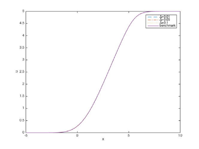
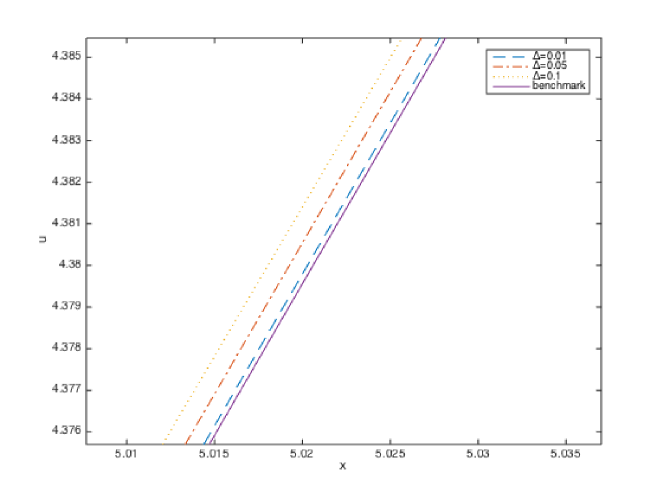
Fig. 1: Approximate values of $u(0,x)$ with various time steps $\Delta=0.01/0.05/0.1$.

Fig. 2: Approximate values of $u(0,x)$ with various time steps $\Delta=0.01/0.05/0.1$. The figure zooms in Fig. 1.1.

Figures 1 and 2 demonstrate the performance of the approximation scheme (20) with the parameter $K=5$. They illustrate how the approximate solutions converge as we increase the number of time steps $T/\Delta$. For our parameter values, $\Delta=0.1$ (so $T/\Delta=10$) is sufficient for the approximate solutions to converge, as the relative error is already negligible ($0.056\%$).

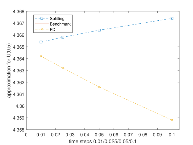
Fig. 3: Comparison of exact value and approximate values for $u(0,5)$ via the approximation scheme (20) and the Howard’s FD scheme with various time steps $\Delta=0.01/0.025/0.05/0.1$.

Figure 3 compares the values numerically computed by the approximation scheme (20) and the Howard’s FD scheme with different time steps. It shows that the approximation scheme gives a better approximation than the Howard’s scheme does. In particular, we observe that when the time step $\Delta=0.1$ (so $T/\Delta=10$), the numerical solution computed by our approximation scheme is far more accurate than the one computed by the FD scheme. The relative error is $0.056\%$ for the former and $0.142\%$ for the latter. It also shows that the approximation scheme converges linearly with time step $\Delta$, and this is consistent with our theoretical results in Theorem 11. Table 1 further compares the computation errors and costs between the approximation scheme (20) and the Howard’s FD scheme. Since there involves an additional minimization step in the approximation scheme (20), its computation costs are higher than the FD scheme. However, we observe that when the time step is small (e.g. $\Delta=0.1$), the computation times for both schemes are extremely fast (less than $0.05$ second).

5 Conclusions

We proposed an approximation scheme for a class of semilinear parabolic equations whose Hamiltonian is convex and coercive to the gradients. The scheme is based on splitting the equation in two parts, the first corresponding to a linear parabolic equation and the second to a Hamilton-Jacobi equation. The solutions of these equations are approximated using, respectively, the Feynman-Kac and the Hopf-Lax formulae. We established the convergence of the approximation scheme and determined the convergence rate, combining Krylov’s shaking coefficients technique and Barles-Jakobsen’s optimal switching approximation. One of the key steps is the derivation of a consistency error via convex duality arguments, using the convexity of the Hamiltonian in an essential way.

The approach and the results herein may be extended in various directions. Firstly, one may consider problem (1) in a bounded domain, an undoubtedly important case since various applications are cast in such domains (e.g. utilities defined in half-space, constrained risk measures, etc.) However, various non-trivial technical difficulties arise. Some recent works on such problems using other approaches can be found in [9], [26] and [34].

Secondly, one may consider variational versions of problem (1). These are naturally related to optimal stopping and to singular stochastic optimization problems, both directly related to various applications with early-exercise, fixed and/or proportional transaction costs, irreversible investment decisions, etc. Recent results in this direction that use some of the ideas developed herein can be found in [21].

Appendix A Proofs of Propositions 2 and 12

We note that equation (1) is a special case (choosing $\varepsilon=0$) of the HJB equation (31). Therefore, we omit the proof of Proposition 2 and only prove Proposition 12.

We first show that there exists a bounded solution to (31). To this end, using the convex dual function $L^{\theta}(t,x,q):=\sup_{p\in\mathbb{R}^{n}}(p\cdot q-H^{\theta}(t,x,p))$, we rewrite (31) as

(49) $$\left\{\begin{array}[]{ll}\displaystyle-\partial_{t}u^{\varepsilon}+{\sup_{\theta\in\Theta^{\varepsilon},q\in\mathbb{R}^{n}}}\mathcal{L}^{\theta,q}\left(t,x,\partial_{x}u^{\varepsilon},\partial_{xx}u^{\varepsilon}\right)=0&\text{in}\ Q_{T+\varepsilon^{2}};\\ \displaystyle u^{\varepsilon}(T+\varepsilon^{2},x)=U(x)&\text{in}\ \mathbb{R}^{n},\end{array}\right.$$

where

$$\mathcal{L}^{\theta,q}(t,x,p,X)=-\frac{1}{2}\text{Trace}\left(\sigma^{\theta}\sigma^{\theta^{T}}(t,x)X\right)-(b^{\theta}(t,x)-q)\cdot p-L^{\theta}(t,x,q).$$

We also introduce the stochastic control problem

$$u^{\varepsilon}(t,x)={\inf_{\theta\in\Theta^{\varepsilon}[t,T+\varepsilon^{2}],q\in\mathbb{H}^{2}[t,T+\varepsilon^{2}]}}\mathbf{E}\left[\int_{t}^{T+\varepsilon^{2}}L^{{\theta_{s}}}\left(s,X_{s}^{t,x;\theta,q},q_{s}\right)ds+U\left(X_{T+\varepsilon^{2}}^{t,x;\theta,q}\right)|\mathcal{F}_{t}\right],$$

with the controlled state equation

$$dX_{s}^{t,x;\theta,q}=\left(b^{{\theta_{s}}}(s,X_{s}^{t,x;\theta,q})-q_{s}\right){ds}+\sigma^{{\theta_{s}}}\left(s,X_{s}^{t,x;\theta,q}\right)dW_{s},$$

where $\Theta^{\varepsilon}[t,T+\varepsilon^{2}]$ is the space of $\Theta^{\varepsilon}$-valued progressively measurable processes $(\tau_{s},e_{s})$ and $\mathbb{H}^{2}[t,T+\varepsilon^{2}]$ is the space of square-integrable progressively measurable processes $q_{s}$, for $s\in[t,T+\varepsilon^{2}]$. Next, we identify its value function with a bounded viscosity solution to (49). For this, we only need to establish upper and lower bounds for the value function $u^{\varepsilon}(t,x)$ and, in turn, use standard arguments as in [33] and [37].

To find an upper bound for $u^{\varepsilon}$, we choose an arbitrary perturbation parameter process $\theta\in\Theta^{\varepsilon}[t,T+\varepsilon]$ and choose $\hat{q}$ with $\hat{q}_{s}\equiv 0$. Then, Proposition 3 (ii) yields

$$u^{\varepsilon}(t,x)\leq \ \mathbf{E}\left[\int_{t}^{T+\varepsilon^{2}}L^{{\theta_{s}}}(s,X_{s}^{t,x;\theta,\hat{q}},0)ds+U(X_{T+\varepsilon^{2}}^{t,x;\theta,\hat{q}})|\mathcal{F}_{t}\right]$$

$$\leq \ (T+\varepsilon^{2}-t)|L^{*}(0)|+M\leq(T+1)|L^{*}(0)|+M.$$

For the lower bound, we use again Proposition 3 (ii) to obtain that $L_{*}(q)\geq-H^{*}(0)\geq-|H^{*}(0)|$, for any $q\in\mathbb{R}^{n}$. In turn, for any $(\theta,q)\in\Theta^{\varepsilon}[t,T+\varepsilon^{2}]\times\mathbb{H}^{2}[t,T+\varepsilon^{2}]$,

$$\ \mathbf{E}\left[\int_{t}^{T+\varepsilon^{2}}L^{{\theta_{s}}}(s,X_{s}^{t,x;\theta,q},q_{s})ds+U(X_{T+\varepsilon^{2}}^{t,x;\theta,q})|\mathcal{F}_{t}\right]$$

$$\geq \ \mathbf{E}\left[\int_{t}^{T+\varepsilon^{2}}L_{*}(q_{s})ds+U(X_{T+\varepsilon^{2}}^{t,x;\theta,q})|\mathcal{F}_{t}\right]$$

$$\geq \ -(T+\varepsilon^{2}-t)|H^{*}(0)|-M\geq-(T+1)|H^{*}(0)|-M,$$

and, thus, $u^{\varepsilon}(t,x)\geq-(T+1)|H^{*}(0)|-M$ and $|u^{\varepsilon}|_{0}\leq C$, for some constant $C$ independent of $\varepsilon$.

The uniqueness of the viscosity solution is a direct consequence of the continuous dependence result, presented next. Its proof follows along similar arguments as in Theorem A.1 of [22] and is thus omitted.

Lemma 17.

For any $s\in(0,{T+\varepsilon^{2}}]$, let $u\in USC(\bar{Q}_{s})$ be a bounded from above viscosity subsolution of (31) with coefficients $\sigma^{\theta},b^{\theta}$ and $H^{\theta}$, and $\bar{u}\in LSC(\bar{Q}_{s})$ be a bounded from below viscosity supersolution of (31) with coefficients $\bar{\sigma}^{\theta},\bar{b}^{\theta}$ and $\bar{H}^{\theta}$. Suppose that Assumption 1 holds for both sets of coefficients with respective constants $M$ and $\bar{M}$, uniformly in $\theta\in\Theta^{\varepsilon}$, and that either $u(s,\cdot)\in\mathcal{C}_{b}^{1}(\mathbb{R}^{n})$ or $\bar{u}(s,\cdot)\in\mathcal{C}_{b}^{1}(\mathbb{R}^{n})$. Then, there exists a constant $C$, depending only on $M$, $\bar{M}$, $[u(s,\cdot)]_{1}$ or $[\bar{u}(s,\cdot)]_{1}$, and $s$, such that, for $(t,x)\in\bar{Q}_{s}$,

(50) $$u-\bar{u}\leq C\left(|(u(s,\cdot)-\bar{u}(s,\cdot))^{+}|_{0}+\sup_{\theta\in\Theta^{\varepsilon}}\left\{|\sigma^{\theta}-\bar{\sigma}^{\theta}|_{0}+|b^{\theta}-\bar{b}^{\theta}|_{0}\right\}+\sup_{\theta\in\Theta^{\varepsilon}}|H^{\theta}-\bar{H}^{\theta}|_{0}\right).$$

The $x$-regularity of $u^{\varepsilon}$ follows easily from (50) by choosing $u=u^{\varepsilon}$, $\bar{u}=u^{\varepsilon}(\cdot,\cdot+e)$ and $s=T+\varepsilon^{2}$.

To get the time regularity, we work as follows. Firstly, let $\rho(x)$ be a $\mathbb{R}_{+}$-valued smooth function with compact support $B(0,1)$ and mass $1$, and introduce the sequence of mollifiers $\rho_{\varepsilon}(x):=\frac{1}{\varepsilon^{n}}\rho\left(\frac{x}{\varepsilon}\right).$ For $0\leq t<s\leq T+\varepsilon^{2}$, let $u_{\varepsilon^{\prime}}$ be the unique bounded solution of (31) in $Q_{s}$ with terminal condition $u_{\varepsilon^{\prime}}(s,x)=u^{\varepsilon}(s,\cdot)*\rho_{\varepsilon^{\prime}}(x)$, for some $\varepsilon^{\prime}>0$. It then follows from (50) that, for $(t,x)\in\bar{Q}_{s}$,

$$u^{\varepsilon}-u_{\varepsilon^{\prime}}\leq C|(u^{\varepsilon}(s,\cdot)-u_{\varepsilon^{\prime}}(s,\cdot))^{+}|_{0}\leq C[u^{\varepsilon}(s,\cdot)]_{1}\varepsilon^{\prime}\leq C\varepsilon^{\prime}.$$

Similarly, we also have $u_{\varepsilon^{\prime}}-u^{\varepsilon}\leq C\varepsilon^{\prime}$.

On the other hand, standard properties of mollifiers imply that $|\partial_{x}^{j}u_{\varepsilon^{\prime}}(s,\cdot)|_{0}\leq C\varepsilon^{\prime 1-j}$. Next, define the functions $w^{+}_{\varepsilon^{\prime}}(t,x):=u_{\varepsilon^{\prime}}(s,x)+(s-t)C_{\varepsilon^{\prime}}$ and $w^{-}_{\varepsilon^{\prime}}(t,x):=u_{\varepsilon^{\prime}}(s,x)-(s-t)C_{\varepsilon^{\prime}}$, where $C_{\varepsilon^{\prime}}=(\frac{1}{\varepsilon^{\prime}}+1)C$, for some constant $C$ independent of $\varepsilon$. We easily deduce that they are, respectively, bounded supersolution and subsolution of (31) in $Q_{s}$, with the same terminal condition $w^{+}_{\varepsilon^{\prime}}(s,x)=w^{-}_{\varepsilon^{\prime}}(s,x)=u_{\varepsilon^{\prime}}(s,x)$. Thus, by (50), we have $w^{-}_{\varepsilon^{\prime}}(t,x)\leq u_{\varepsilon^{\prime}}(t,x)\leq w^{+}_{\varepsilon^{\prime}}(t,x),$ for $(t,x)\in\bar{Q}_{s}$, which in turn implies that $|u_{\varepsilon^{\prime}}(t,x)-u_{\varepsilon^{\prime}}(s,x)|\leq C_{\varepsilon^{\prime}}|s-t|.$ Choosing $\varepsilon^{\prime}=\sqrt{|s-t|}$, we then obtain that

$$|u^{\varepsilon}(t,x)-u^{\varepsilon}(s,x)|\leq \ |u^{\varepsilon}(t,x)-u_{\varepsilon^{\prime}}(t,x)|+|u_{\varepsilon^{\prime}}(t,x)-u_{\varepsilon^{\prime}}(s,x)|+|u_{\varepsilon^{\prime}}(s,x)-u^{\varepsilon}(s,x)|$$

$$\leq \ 2C\varepsilon^{\prime}+C_{\varepsilon^{\prime}}|s-t|\leq C(\varepsilon^{\prime}+\frac{|s-t|}{\varepsilon^{\prime}}+|s-t|)\leq C\sqrt{|s-t|},$$

which, together with the boundedness and the $x$-regularity of $u^{\varepsilon}$, implies that $|u^{\varepsilon}|_{1}\leq C$.

Finally, note that $u(t,x)$ is also the bounded viscosity solution of (31) when $\sigma^{\theta}\equiv\sigma$, $b^{\theta}\equiv b$ and $H^{\theta}\equiv H$. Applying (50) once more and using the regularity of $\sigma$, $b$, $H$ and $u^{\varepsilon}$, we deduce that

$$u^{\varepsilon}-u\leq \ C\left(|(u^{\varepsilon}(T,\cdot)-u(T,\cdot))^{+}|_{0}+\sup_{\theta\in\Theta^{\varepsilon}}\left\{|\sigma^{\theta}-\sigma|_{0}+|b^{\theta}-b|_{0}\right\}+\sup_{\theta\in\Theta^{\varepsilon}}|H^{\theta}-H|_{0}\right)$$

$$\leq \ C\left(|u^{\varepsilon}(T,\cdot)-u^{\varepsilon}(T+\varepsilon^{2},\cdot)|_{0}+\varepsilon\right)\leq C\varepsilon\ \ \text{in}\ \bar{Q}_{T}.$$

Similarly, we also have $u-u^{\varepsilon}\leq C\varepsilon$, and we easily conclude.

	$0.01$	$0.25$	$0.05$	$0.1$
splitting approx. value	4.3655	4.3658	4.3664	4.3674
approx. error	0.012%	0.02%	0.032%	0.056%
running time (in seconds)	18.78	1.07	0.16	0.04
FD approx. value	4.3642	4.3632	4.3616	4.3588
approx. error	0.016%	0.039%	0.076%	0.142%
running time (in seconds)	7.01	0.43	0.03	0.01

Table 1: Comparison of running errors and costs for approximating $u(0,5)$ via the approximation scheme (20) and the Howard’s FD scheme with various time steps $\Delta=0.01/0.025/0.05/0.1$.

References

• [1] Barles, G. and E. R. Jakobsen. Error bounds for monotone approximation schemes for Hamilton-Jacobi-Bellman equations. SIAM Journal on Numerical Analysis, 43(2): 540-558, 2005.
• [2] Barles, G. and E. R. Jakobsen. Error bounds for monotone approximation schemes for parabolic Hamilton-Jacobi-Bellman equations. Mathematics of Computation, 76: 1861-1893, 2007.
• [3] Barles, G. and E. R. Jakobsen. On the convergence rate of approximation schemes for Hamilton-Jacobi-Bellman equations. M2AN Math. Model. Numer. Anal., 36(1): 33-54, 2002.
• [4] Barles, G. and P. E. Souganidis. Convergence of approximation schemes for fully nonlinear second order equations. Asymptotic Analysis, 4(3): 271–283, 1991.
• [5] Bayraktar, E. and A. Fahim. A stochastic approximation for fully nonlinear free boundary problems. Numerical Methods for Partial Differential Equations, 30(3): 902-929, 2014.
• [6] Bokanowski, O., S. Maroso, and H. Zidani. Some convergence results for Howard’s algorithm. SIAM Journal on Numerical Analysis, 47(4): 3001-3026, 2009.
• [7] Bokanowski, O., A. Picarelli, and H. Zidani. Dynamic programming and error estimates for stochastic control problems with maximum cost. Applied Mathematics & Optimization, 71(1): 125-163, 2015.
• [8] Bouchard, B. and N. Touzi. Discrete-time approximation and Monte-Carlo simulation of backward stochastic differential equations. Stochastic Processes and their Applications, 111(2), 175–206, 2004.
• [9] Caffarelli, L.A. and P. E. Souganidis. A rate of convergence for monotone finite difference approximations to fully nonlinear uniformly elliptic PDEs. Communications on Pure and Applied Mathematics, 61(1):1-7, 2008.
• [10] Chassagneux, J.F. and A. Richou. Numerical simulation of quadratic BSDEs. The Annals of Applied Probability, 26(1): 262–304, 2016.
• [11] Chong, W.F., Y. Hu, G. Liang and T. Zariphopoulou. An ergodic BSDE approach to forward entropic risk measures: representation and large-maturity behavior. Finance and Stochastics, 23(1): 239–273, 2019.
• [12] Delbaen, F., Y. Hu, and X. Bao. Backward SDEs with superquadratic growth. Probability Theory and Related Fields, 150(1), 145-192, 2011.
• [13] El Karoui, N. and R. Rouge. Pricing via utility maximization and entropy. Mathematical Finance 10, 259–276. 2000.
• [14] Evans, L. C. Partial Differential Equations. Graduate Studies in Mathematics, Americal Mathematical Society, 1998.
• [15] Evans, L. C. and A. Friedman. Optimal stochastic switching and the Dirichlet problem for the Bellman equation. Trans. Amer. Math. Soc, 253:365-389, 1979.
• [16] Fahim A., N. Touzi, and X. Warin. A probabilistic numerical method for fully nonlinear parabolic PDEs. The Annals of Applied Probability, 21: 1322–1364, 2011.
• [17] Giles, M. B. Multilevel monte carlo path simulation. Operations Research, 56(3), 607–617, 2008.
• [18] Henderson, V. and G. Liang. Pseudo linear pricing rule for utility indifference valuation. Finance and Stochastics, 18(3):593–615, 2014.
• [19] Henderson, V. and G. Liang. A multidimensional exponential utility indifference pricing model with applications to counterparty risk. SIAM Journal on Control and Optimization, 54(3): 690–717, 2016.
• [20] Hu, Y., P. Imkeller and M. Müller. Utility maximization in incomplete markets. The Annals of Applied Probability, 15: 1691–1712, 2005.
• [21] Huang, S. An approximation scheme for variational inequalities with convex and coercive Hamiltonians. Working paper, 2018, arXiv:1810.08842.
• [22] Jakobsen, E. R. On the rate of convergence of approximation schemes for Bellman equations associated with optimal stopping time problems. Math. Models Methods Appl. Sci., 13(5): 613-644, 2003.
• [23] Kobylanski, M. Backward stochastic differential equations and partial differential equations with quadratic growth. The Annals of Probability, 28: 558–602, 2000.
• [24] Krylov, N. V. On the rate of convergence of finite-difference approximations for Bellman’s equation. St. Petersburg Math. J., 9(3):639-650, 1997.
• [25] Krylov, N. V. On the rate of convergence of finite-difference approximations for Bellman’s equations with variable coefficients. Probability Theory and Related Fields, 117(1): 1-16, 2000.
• [26] Krylov, N. V. On the rate of convergence of finite-difference approximations for elliptic Isaacs equations in smooth domains. Communications in Partial Differential Equations, 40(8): 1393-1407, 2015.
• [27] Lions, P. L. and B. Mercier. Splitting algorithms for the sum of two nonlinear operators. SIAM Journal on Numerical Analysis, 16(6): 964-979, 1979.
• [28] Longstaff, F. A. and E. S. Schwartz. Valuing American options by simulation: a simple least-squares approach. The Review of Financial Studies, 14(1), 113-147, 2001.
• [29] Lyons, T. and N. Victoir. Cubature on Wiener space. Proceedings of the Royal Society of London. Series A: Mathematical, Physical and Engineering Sciences, 460(2041), 169–198, 2004.
• [30] Marchuk, G. I. Some application of splitting-up methods to the solution of mathematical physics problems. Apl. Mat., 13: 103-132, 1968.
• [31] Nadtochiy, S. and T. Zariphopoulou. An approximation scheme for solution to the optimal investment problem in incomplete markets. SIAM J. Finan. Math., 4(1): 494-538, 2013.
• [32] Nelder, J. A. and R. Mead. A simplex method for function minimization. Computer Journal, 7: 308-313, 1965.
• [33] Pham, H. Continuous-time Stochastic Control and Optimization with Financial Applications. Springer, 2009.
• [34] Picarelli, A., C. Reisinger, and J. Rotaetxe Arto. Error bounds for monotone schemes for parabolic Hamilton-Jacobi-Bellman equations in bounded domains. Working paper, 2017, arXiv:1710.11284.
• [35] Tan X. A splitting method for fully nonlinear degenerate parabolic PDEs. Electron. J. Probab., 18(15): 1-24, 2013.
• [36] Tourin, A. Splitting methods for Hamilton-Jacobi equations, Numerical Methods Partial Differential Equations, 22: 381-396, 2006.
• [37] Touzi, N. Optimal Stochastic Control, Stochastic Target Problems, and Backward SDE. Springer, 2012.
• [38] Zariphopoulou, T., A solution approach to valuation with unhedgeable risks, Finance and Stochastics, 5(1): 61–82, 2001.
Refer to caption