Tail empirical process and weighted extreme value index estimator for randomly right-censored data
Brahim Brahimi, Djamel Meraghni, Abdelhakim Necir∗, Louiza Soltane
Laboratory of Applied Mathematics, Mohamed Khider University, Biskra, Algeria
Abstract
A tail empirical process for heavy-tailed and right-censored data is introduced and its Gaussian approximation is established. In this context, a (weighted) new Hill-type estimator for positive extreme value index is proposed and its consistency and asymptotic normality are proved by means of the aforementioned process in the framework of second-order conditions of regular variation. In a comparative simulation study, the newly defined estimator is seen to perform better than the already existing ones in terms of both bias and mean squared error. As a real data example, we apply our estimation procedure to evaluate the tail index of the survival time of Australian male Aids patients. It is noteworthy that our approach may also serve to develop other statistics related to the distribution tail such as second-order parameter and reduced-bias tail index estimators. Furthermore, the proposed tail empirical process provides a goodness-of-fit test for Pareto-like models under censorship.
Keywords: Extreme value index; Heavy tails; Random censoring; Tail empirical process.
AMS 2010 Subject Classification: 60F17, 62G30, 62G32, 62P05.
Corresponding author:
necirabdelhakim@yahoo.fr
E-mail
addresses:
brah.brahim@gmail.com (B. Brahimi)
djmeraghni@yahoo.com (D. Meraghni)
louiza_stat@yahoo.com (L. Soltane)
1. Introduction
Let be independent copies of a non-negative continuous random variable (rv) defined over some probability space with cumulative distribution function (cdf) These rv’s are censored to the right by a sequence of independent copies of a non-negative continuous rv independent of and having a cdf At each stage we only can observe the rv’s and with denoting the indicator function. The latter rv indicates whether there has been censorship or not. If we denote by the cdf of the observed then, in virtue of the independence of and we have Throughout the paper, we will use the notation for any Assume further that and are heavy-tailed or, in other words, that and are regularly varying at infinity with negative indices and respectively, notation: and That is
| (1.1) |
as for any This class of distributions includes models such as Pareto, Burr, Fréchet, stable t-Student and log-gamma, known to be very appropriate for fitting large insurance claims, large fluctuations of prices, financial log-returns, … (see, e.g., Resnick, 2006). The regular variation of and implies that where Since weak approximations of extreme value theory based statistics are achieved in the second-order framework (see de Haan and Stadtmüller, 1996), then it seems quite natural to suppose that cdf satisfies the well-known second-order condition of regular variation: for any
as where is the second-order parameter and is a function tending to not changing sign near infinity and having a regularly varying absolute value at infinity with index If interpret as Let us denote this assumption by For the use of second-order conditions in exploring the estimators asymptotic behaviors, see, for instance, Theorem 3.2.6 in de Haan and Ferreira (2006), page 74. In the last decade, several authors showed an increasing interest in the issue of estimating the extreme-value index (EVI) when the data are subject to random censoring. In this context, Beirlant et al. (2007) proposed estimators for the EVI and high quantiles and discussed their asymptotic properties, when the observations are censored by a deterministic threshold, while Einmahl et al. (2008) adapted various classical EVI estimators to the case where the threshold of censorship is random, and proposed a unified method to establish their asymptotic normality. Here, we remind the adjustment they made to Hill estimator (Hill, 1975) so as to estimate the tail index under random censorship. Let be a sample from the couple of rv’s and represent the order statistics pertaining to If we denote the concomitant of the th order statistic by (i.e. if then the adapted Hill estimator of defined by Einmahl et al. (2008), is given by the formula where
| (1.2) |
for a suitable sample fraction are respectively Hill’s estimator (Hill, 1975) of and an estimator of the proportion of the observed extreme values. By following similar procedures, Ndao et al. (2014, 2016) addressed the nonparametric estimation of the conditional EVI and large quantiles for heavy-tailed distributions which was generalized, a couple of years later, by Stupfler (2016) to all three extreme domains of attraction namely, Féchet, Gumbel and Weibull types of distributions. In his working paper Stupfler (2017) considered the dependent random right-censoring scheme and develop an interesting new topic. For their part, Worms and Worms (2014) used Kaplan-Meier integration and the synthetic data approach of Leurgans (1987), to respectively introduce two Hill-type estimators
and
where
| (1.3) |
is the famous Kaplan-Meier estimator of cdf (Kaplan and Meier, 1958). In their simulation study, the authors pointed out that, for weak censoring their estimators perform better than in terms of bias and mean squared error. However, in the strong censoring case they noticed that the results become unsatisfactory for both and With additional assumptions on and they only established the consistency of their estimators, without any indication on the asymptotic normality. Though these conditions are legitimate from a theoretical viewpoint, they may be considered as constraints in case studies. Very recently, Beirlant et al. (2018) used Worms’s estimators to derive new reduced-bias ones, constructed bootstrap confidence intervals for and applied their results to long-tailed car insurance portfolio. Likewise, Beirlant et al. (2016) considered maximum likelihood inference, on the basis of the relative excesses to propose a new reduced-bias estimator for the tail index of models belonging to Hall’s class (Hall, 1982). The problem is that, even if this family includes a great number of usual heavy-tailed distributions, it represents a restriction to the larger class of regularly varying cdf’s, in particular those with null second-order parameter such as the log-gamma model. As we can see, the only EVI estimator that does not impose any restrictive assumptions on the model is the one introduced by Einmahl et al. (2008). For this reason, we intend to construct a new weighted estimator to the index that enjoys the benefits of
1.1. Constructing a new estimator for
First, we introduce two very crucial sub-distribution functions for so that one has The empirical counterparts are, respectively, defined by
and From Lemma 4.1 of Brahimi et al. (2015), under the first-order conditions we have as which implies that too. Then it is natural to also assume that satisfies the second-order condition of regular variation, in the sense that From Theorem 1.2.2 in de Haan and Ferreira (2006), the assumption implies that as which, by integration by parts, gives
| (1.4) |
In other words, we have
Taking and replacing and by their respective empirical counterparts and yield that becomes, in terms of
| (1.5) |
We have and then it is readily checked that
Substituting this in leads to the definition of By incorporating the quantity inside the integral we get from Lemma 7.1 (for
But one has to be careful, because a division by zero may occur in the estimation procedure. Indeed, we have for instance which may be or To avoid this boring situation, we add to the denominator a suitable non-null sequence tending to zero and being in agreement with the normalizing constant corresponding to the limit distributions of tail indices estimators. For convenience, to have Gaussian approximations of order (tending to zero in probability), we choose the sequence and we show in Lemma 7.1, that for a given sequence we have
| (1.6) |
Thus, by letting and by replacing and by and respectively, the left-hand side becomes
This may be rewritten into
which equals
Finally, changing by and by yields a new (random) weighted estimator for the EVI as follows:
| (1.7) |
For the purpose of establishing the consistency and asymptotic normality of we next introduce a tail empirical process for censored data. For let us define
| (1.8) |
By integrating by parts, we show easily that thereby, motivated by the tail product-limit process for truncated data, recently given in Benchaira et al. (2016a), we defined this tail empirical process by
| (1.9) |
so that
In the non censoring case we have with being the usual empirical cdf. In this case, we have
thus
| (1.10) |
corresponds (asymptotically) to the tail empirical process for complete data (see, e.g., page 161 in de Haan and Ferreira, 2006). Note that one may think that it would have been more natural to simply use Kaplan-Meier estimator of given in to define a tail empirical process in the censoring case. This was done in Brahimi et al. (2016), but the asymptotic properties were only established under the condition which would constitute a restriction for applications. Indeed, there exist real datasets used in case studies with proportions estimated at less than a half. We can cite, amongst others, the aids survival data to which Einmahl et al. (2008) applied their methodology and approximately got for (it is exacly the same value that we ourselves will find later on in Section 4) and the car liability insurance data studied in Beirlant et al. (2016) and Beirlant et al. (2018) where the estimated value of was
The rest of the paper is organized as follows. In Section 2, we provide our main result, namely two weak approximations leading to consistency and asymptotic normality of whose proofs are postponed to Section 5. The finite sample behavior of the proposed estimator is checked by simulation in Section 3, where a comparison with the already existing ones is made as well. Section 4 is devoted to an application to the survival time of Australian male Aids patients. Finally, some results that are instrumental to the proofs are given in the Appendix.
2. Main results
In the sequel, the functions and respectively stand for the quantile and tail quantile functions pertaining to cdf For further use, we set and define
| (2.11) |
Let us now state our first result in which we provide Gaussian approximations both to and
Theorem 2.1.
Assume that and and let be an integer sequence such that and Then there exists a sequence of Brownian bridges defined on the probability space such that, for every we have
| (2.12) |
as where is a centred Gaussian process defined by
with for If, in addition, we assume that
then
| (2.13) |
as where
with and provided that and
In the following theorem, we establish the consistency and asymptotic normality of our new estimator
Theorem 2.2.
Assume that and and let be an integer sequence such that and then as If, in addition, we assume that and so that and be asymptotically bounded, then
where
| (2.14) |
Whenever and respectively converge to finite real numbers and then
where
with
Remark 2.1.
It is to be noted that for distributions in Hall’s class of models, (Hall, 1982), the three assumptions and may be gathered in a single one, namely which is already used by Beirlant et al. (2016) in Theorem 1, written as where Indeed, let us assume that both and belong to this family, which contains the most popular heavy-tailed cdf’s, such as Burr, Fréchet, Generalized Pareto, Generalized Extreme Value, t-Student, … Explicitly, there exist constants and such that, as
and
This implies that we have, as
and
where
It is easy to check that both and satisfy the second-order condition of regular variation with convergence rates and respectively. Moreover, we have and therefore In this context, as thus as Consequently, by replacing by we get that and are indeed all of convergence rate
Remark 2.2.
3. Simulation study
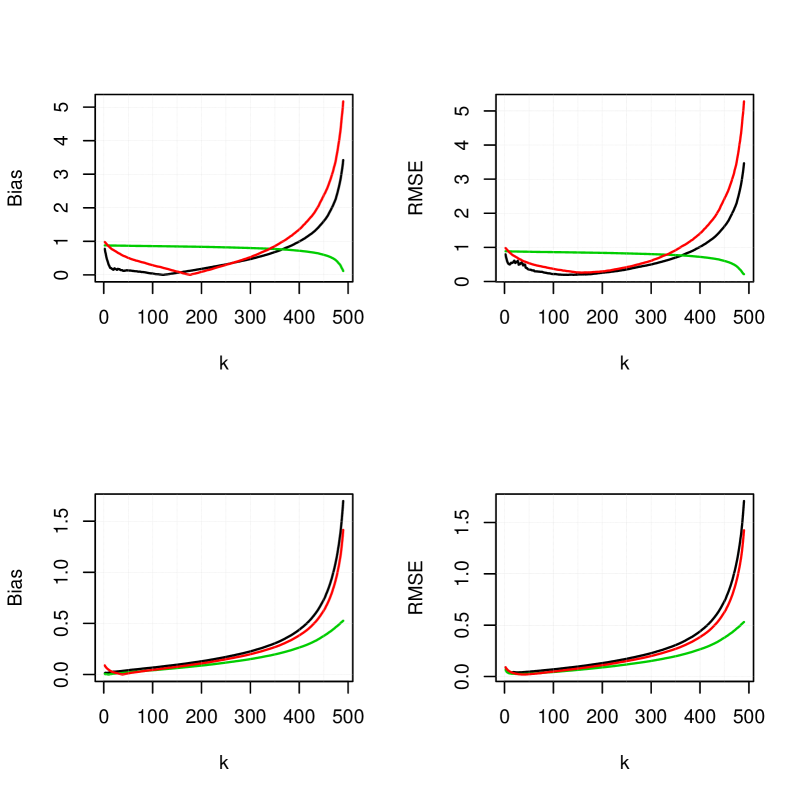
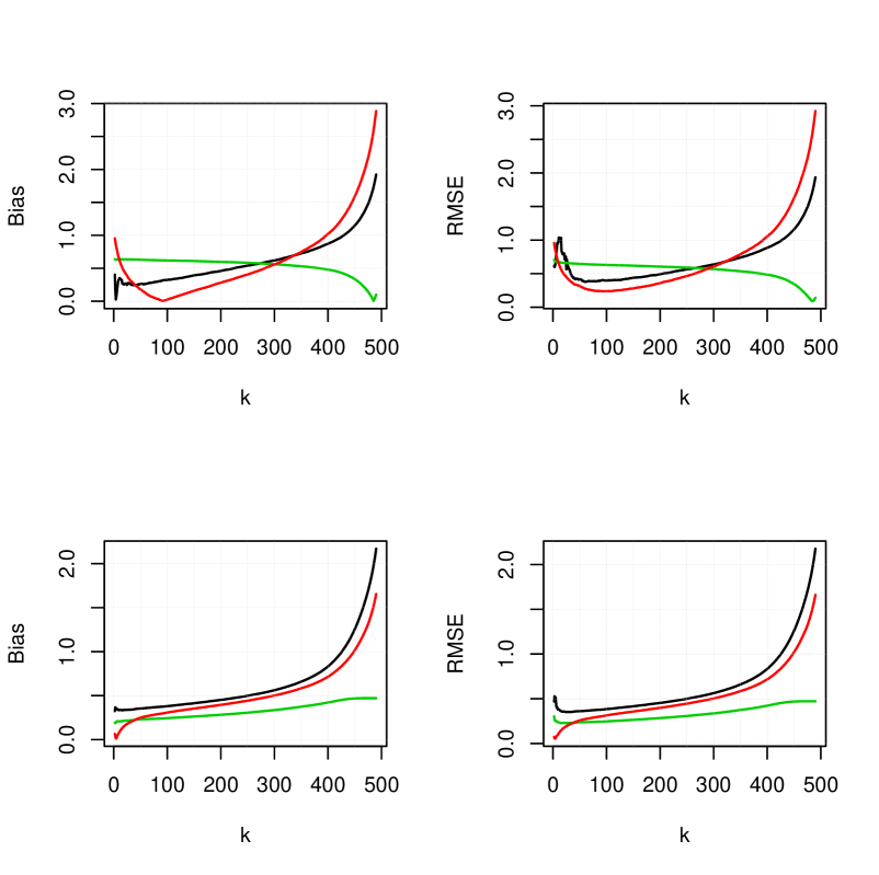
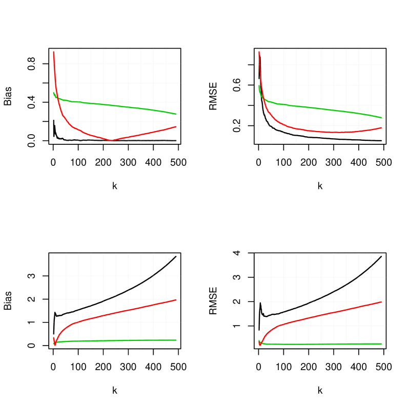
Now, we carry out an extensive simulation study to illustrate the behavior of the proposed estimator and compare its performance, in terms of (absolute) bias and root of the mean squared error (RMSE), with those of and To this end, we consider Burr’s, Fréchet’s and the log-gamma models respectively defined, for by:
-
•
Burr for with
-
•
Fréchet for
-
•
log-gamma for and
We select two values, and for the proportion of observed upper statistics and we make several combinations of the parameters of each model. For each case, we generate samples of size and we take our overall results (given in the form of graphical representations) by averaging over all independent replications. We consider three censoring schemes, namely Burr censored by Burr, Fréchet censored by Fréchet and log-gamma censored by log-Gamma, that we illustrate by Figures 3.1, 3.2 and 3.3 respectively. In each figure, we represent the biases and the RMSE’s of all three estimators and as functions of the number of the largest order statistics. Our overall conclusion is that, from the top panels of all three figures, we see that the newly proposed estimator and the adapted Hill one perform almost equally well and better than Worms’s estimator in the strong censoring case. However, the bottom panels of Figure 3.1 and Figure 3.2 show that, for the weak censoring scenario, the latter has a slight edge (especially for small values of over the other two which still behave almost similarly. This agrees with the conclusion of B17 and means that is not reliable enough in the strong censoring situation. We notice, from Figure 3.3, that when considering the log-gamma model with strong censoring, the estimator outperforms the remaining two. But, with weak censoring, is clearly better than while does not even work in this case, which is something of very striking.
4. Application to Australian Aids data
The data file consists in Australian patients who were diagnosed with Aids on July 1991. The file contains the identification number, the dates of first diagnosis, birth and death, as well as the state and the encrypted transmission category. The data are available in the package ”MASS” of the statistical software R. Our objective is to apply the newly proposed estimation procedure to evaluate the tail index of the survival time of the patients. To this end, we first select the optimal number of top statistics used in the estimate computation. By applying the adaptive algorithm of Reiss and Thomas (see, Reiss and Thomas (2007), page 137), we find that extreme observations are needed to obtain a proportion estimate value This represents a strong censoring rate of around for which is not recommended for the estimation of the tail index as seen in Section 3. Therefore, we only compute the other two estimates and for which the abovementioned technique gives and respectively. Note that this latter value differs from that found by Einmahl et al. (2008) who used a graphical approach which is not as objective as a numerical procedure.
5. Proofs
5.1. Preliminaries
Let be a sequence of iid rv’s uniformly distributed on (Einmahl and Koning, 1992), and define the corresponding empirical cdf and empirical process by
| (5.15) |
respectively. Thereby, we may represent, almost surely, both and in term of as follows
| (5.16) |
and
| (5.17) |
For more details, one refers to Deheuvels and Einmahl (1996). Therefore, in view of the previous representations, we have almost surely
| (5.18) |
and
| (5.19) |
Our methodology strongly relies on the well-known Gaussian approximation, given by Csörgő et al. (1986) in Corollary 2.1, which says that on the probability space there exists a sequence of Brownian bridges such that for every and
| (5.20) |
For the increments we will need an approximation of the same type as Following similar arguments, mutatis mutandis, as those used to in the proof of assertions of Theorem 2.1 and of Theorem 2.2 in Csörgő et al. (1986), Necir (2017), recently showed, in a technical report, that for every and one also has
| (5.21) |
5.2. Proof of Theorem 2.1
To get the asymptotic weak approximation given in Theorem 2.1, we will perform successive decompositions that will produce several remainder terms We show, in Lemmas 7.6, 7.8, 7.9, 7.10, 7.12, 7.13 and 7.14 of the Appendix, that for a every fixed and for all large we have for uniformly over Then, once one of the remainder terms appears in the following decompositions it is systematically replaced by Let us begin by setting and rewrite both and into
Observe now that may be rewritten into
In view of Taylor’s expansion, we write then by using this latter twice, for and we may decompose into the sum of
and three remainder terms
and
Let us now also decompose into the sum of
and
For the purpose of establishing Gaussian approximations to we introduce the following two crucial tail empirical processes and defined, for by
| (5.22) |
and
| (5.23) |
5.2.1. Asymptotic representations to in terms of and
Let us now decompose into the sum of
and
The change of variable and the definition yield that
and
The term may in turn be decomposed into
and
Thus, we end up with
Now, we use similar decompositions to the second term Observe that this latter equals
plus a remainder term
Likewise, may be rewritten as the sum of
and
Thereby
For the third term we make a change of variables and an integration by parts to get
Making use of Lemma 7.3, we get The fourth term may in turn be rewritten as the sum of
plus two remainder terms
and
Note that is asymptotically Gaussian, it follows that and (see, for instance, Theorem 2.1 (assertion 2.7) in Brahimi et al., 2015). On the other hand, from proposition 7.1 (see the Appendix), we infer that Then, by using the mean value theorem, in yields
From assertion in Brahimi et al. (2015), we have it follows that
To summarize, we showed that
where
| (5.24) |
and
In the following Section we provide Gaussian approximations to
5.3. Gaussian approximation to
We show that
| (5.25) |
| (5.26) |
and
| (5.27) |
where is the centred Gaussian process given in Theorem 2.1. We will only give details for since the proofs of and follow by using similar arguments. Let us also introduce the following Gaussian processes that we define, for by
| (5.28) |
It is clear that given in may be rewritten as the sum of
and two remainder terms
and
Let us now focus on the term Since then for it follows that for therefore
Let be the empirical quantile function pertaining to cdf For convenience, we set
| (5.29) |
and make the change of variable to get
In view of the algebraic equation we decompose into the sum of
and three remainder terms
and
Let us also decompose into the sum of
and
Finally, we end up
which meets with approximation Recall that in Theorem 2.1, we set
this means that therefore
uniformly over this completes the proof of weak approximation
5.4. Gaussian approximation to
Recall that which may be rewritten into the sum of
In view of weak approximation it suffices to show that meets the remainder term Indeed, by letting we write
which in turn may be decomposed into the sum of
and
where By using the uniform inequalities (for the second-order regularly varying functions) to (see, e.g., de Haan and Ferreira, 2006, bottom of page 161) we write: for any there exists such that for all and
Recall that, by assumption, we have it follows that
For the second and third terms, let us write
Making use of Lemma 7.2 and Proposition 7.1 (applied to with the fact that and we end up, after integration, with
For the third term, we also assumed that then it suffices to use on again Proposition 7.1 to readily get as sought.
5.5. Proof of Theorem 2.2
Let us begin by the consistency of which may be rewritten into and write
where
It is clear that for a fixed we have
Since (finite), then by using weak approximation given in Theorem 2.1, we end up with On the other hand is a centred Gaussian random with variance
By a tedious (but elementary) computation we show that A similar calculation may be found in the proof of Corollary 2.1 of Brahimi et al. (2015). It remains to show that as Indeed, we have
By an integration by parts, this latter becomes
which, from Lemma 7.1, tends to as as sought. Let us now consider the asymptotic normality. Recall that and use the weak approximation to get
where By using integrations by parts with elementary calculations, we show that meets formula and
with variance tending to which leads to the Gaussian approximation and therefore the asymptotic normality of
6. Concluding notes
In this work, we first defined a tail empirical process for Pareto-like distributions which are randomly right-censored and established its Gaussian approximation. The latter will play a central role, in the context of right censorship, in determining the asymptotic distributions of statistics that are functionals of the tail index estimator such as the estimators of large quantiles, risk measures, second-order parameters of regular variation… Then, we introduced a new Hill-type estimator for positive EVI of right-censored heavy-tailed data whose asymptotic behavior (consistency and asymptotic normality) is assessed by using the above-mentioned tail process. Compared to other existing estimators, the new tail index estimator performs better, as far as bias and mean squared error are concerned, at least from a simulation viewpoint. As a case study, we provided an estimator to the survival time of Australian male Aids patients. It is also worth mentioning, that assumption also implies that
where is a suitable weight function and is some positive real number. Thus, assertion becomes a special case of the limit above. Thereby, the functional can be considered as a basic tool to constructing a whole class of estimators for distribution tail parameters for complete data, see for instance Ciuperca and Mercadier (2010). Recently, Benchaira et al. (2016a) and Haouas et al. (2017) benefited from this result to derive, respectively, a kernel estimator of tail index and a second-order parameter estimator for random right-truncation data. As we deal with the tail modeling of underlying cdf we have to work with the limit
which is generalization of the result This latter may be readily shown by using similar arguments as those used in Lemma 7.2. Thereby, by letting then by replacing and by their respective empirical counterparts and we end up with an estimator of given by
where This would have fruitful consequences on the statistical analysis of extremes under random censoring. To finish, notice that the Gaussian approximations corresponding to and are jointly established in terms of the same sequence of Brownian bridges This allows to establish the limit distributions to the statistics of Kolmogorov-Smirnov and Cramer-von Mises type respectively defined by
and
These statistics provide goodness-of-fit tests for Pareto-like distributions under right-censorship. This matter will be addressed in our future work. In the case of complete data the latter two statistics respectively become
They are used in Koning and Peng, (2008), amongst others, to test the heaviness of cdf’s.
References
- Beirlant et al. (2007) Beirlant, J., Guillou, A., Dierckx, G., Fils-Villetard, A., 2007. Estimation of the extreme value index and extreme quantiles under random censoring. Extremes 10, 151-174.
- Beirlant et al. (2016) Beirlant, J., Bardoutsos, A., de Wet, T., Gijbels, I., 2016. Bias reduced tail estimation for censored Pareto type distributions. Statist. Probab. Lett. 109, 78-88.
- Beirlant et al. (2018) Beirlant, J., Maribe, G., Verster, A., 2018. Penalized bias reduction in extreme value estimation for censored Pareto-type data, and long-tailed insurance applications. Insurance Math. Econom., 78, 114-122.
- Benchaira et al. (2016a) Benchaira, S., Meraghni, D., Necir, A., 2016. Tail product-limit process for truncated data with application to extreme value index estimation. Extremes, 19, 219-251.
- Benchaira et al. (2016b) Benchaira, S., Meraghni, D., Necir, A., 2016. Kernel estimation of the tail index of a right-truncated Pareto-type distribution. Statist. Probab. Lett. 119, 186-193.
- Bingham et al. (1987) Bingham, N. H., Goldie, C. M., Teugels, J. L., 1987. Regular Variation. Cambridge University Press.
- Brahimi et al. (2015) Brahimi, B., Meraghni, D., Necir, A., 2015. Approximations to the tail index estimator of a heavy-tailed distribution under random censoring and application. Math. Methods Statist. 24, 266-279.
- Brahimi et al. (2016) Brahimi, B., Meraghni, D., Necir, A., 2016. Nelson-Aalen tail product-limit process and extreme value index estimation under random censorship. ArXiv: https://arxiv.org/abs/1502.03955v2.
- Ciuperca and Mercadier (2010) Ciuperca, G., Mercadier, C., 2010. Semi-parametric estimation for heavy tailed distributions. Extremes 13:55-87.
- Csörgő and Révész, (1981) Csörgő, M., Révész, P., 1981. Strong approximations in probability and statistics. Probability and Mathematical Statistics. Academic Press, Inc. [Harcourt Brace Jovanovich, Publishers], New York-London.
- Csörgő et al. (1985) Csörgő, S., Deheuvels, P., Mason, D., 1985. Kernel estimates of the tail index of a distribution. Ann. Statist. 13, 1050-1077.
- Csörgő et al. (1986) Csörgő, M., Csörgő, S., Horváth, L., Mason, D. M., 1986. Weighted empirical and quantile processes. Ann. Probab. 14, 31-85.
- Csörgő (1996) Csörgő, S. (1996). Universal Gaussian approximations under random censorship. Ann. Statist. 24, 2744-2778.
- Deheuvels and Einmahl (1996) Deheuvels, P., Einmahl, J. H. J., 1996. On the strong limiting behavior of local functionals of empirical processes based upon censored data. Ann. Probab. 24, 504-525.
- Einmahl et al. (2006) Einmahl, J. H. J., de Haan, L., Li, D., 2006. Weighted approximations of tail copula processes with application to testing the bivariate extreme value condition. Ann. Statist. 34, 1987-2014.
- Einmahl et al. (2008) Einmahl, J. H. J., Fils-Villetard, A., Guillou, A., 2008. Statistics of extremes under random censoring. Bernoulli 14, 207-227.
- Einmahl and Koning (1992) Einmahl, J. H. J., Koning, A. J., 1992. Limit theorems for a general weighted process under random censoring. Canad. J. Statist. 20, 77-89.
- Haouas et al. (2017) Haouas, N., Necir, A., Brahimi, B., 2017. Estimating the second-order parameter of regular variation and bias reduction in tail index estimation under random truncation . ArXiv: hhttps://arxiv.org/abs/1610.00094
- Hua and Joe (2011) Hua, L., Joe, H., 2011. Second order regular variation and conditional tail expectation of multiple risks. Insurance Math. Econom. 49, 537-546.
- de Haan and Resnick (1993) de Haan, L., Resnick, S.., 1993. Estimating the limit distribution of multivariate extremes. Comm. Statist. Stochastic Models 9, 275-309.
- de Haan and Stadtmüller (1996) de Haan, L., Stadtmüller, U., 1996. Generalized regular variation of second order. J. Australian Math. Soc. (Series A) 61, 381-395.
- de Haan and Resnick (1998) de Haan, L., Resnick, S., 1998. On asymptotic normality of the Hill estimator. Comm. Statist. Stochastic Models 14, 849-866.
- de Haan and Ferreira (2006) de Haan, L., Ferreira, A., 2006. Extreme Value Theory: An Introduction. Springer.
- Hall (1982) Hall, P., 1982. On some simple estimates of an exponent of regular variation. Journal of the Royal Statistical Society 44, 37-42.
- Hill (1975) Hill, B. M., 1975. A simple general approach to inference about the tail of a distribution. Ann. Statist. 3, 1163-1174.
- Kaplan and Meier (1958) Kaplan, E. L., Meier, P., 1958. Nonparametric estimation from incomplete observations. J. Amer. Statist. Assoc. 53, 457-481.
- Koning and Peng, (2008) Koning, A.J., Peng, L., 2008. Goodness-of-fit tests for a heavy tailed distribution. J. Statist. Plann. Inference 138: 3960-3981.
- Leurgans (1987) Leurgans, S., 1987. Linear models, random censoring and synthetic data. Biometrika 74, 301-309.
- Ndao et al. (2014, 2016) Ndao, P., Diop, A., Dupuy, J.-F., 2014. Nonparametric estimation of the conditional tail index and extreme quantiles under random censoring. Comput. Statist. Data Anal. 79, 63–79.
- Ndao et al. (2015) Ndao, P., Diop, A., Dupuy, J.-F., 2016. Nonparametric estimation of the conditional extreme-value index with random covariates and censoring. J. Statist. Plann. Inference 168, 20-37.
- Necir (2017) Necir, A., 2017. Komlós-Major-Tusnády approximations to increments of uniform empirical processes. ArXiv: https://arxiv.org/abs/1709.00747v2.
- Reiss and Thomas (2007) Reiss, R.-D., Thomas, M., 2007. Statistical Analysis of Extreme Values with Applications to Insurance, Finance, Hydrology and Other Fields, 3rd ed. Birkhäuser Verlag, Basel, Boston, Berlin.
- Resnick (2006) Resnick, S., 2006. Heavy-Tail Phenomena: Probabilistic and Statistical Modeling. Springer.
- Shorack and Wellner (1986) Shorack, G. R., Wellner, J. A., 1986. Empirical Processes with Applications to Statistics. Wiley.
- Stupfler (2016) Stupfler, G., 2016. Estimating the conditional extreme-value index under random right-censoring. J. Multivariate Anal. 144, 1-24.
- Stupfler (2017) Stupfler, G., 2017. On the study of extremes with dependent random right-censoring. Working paper: https://hal.archives-ouvertes.fr/hal-01450775/document.
- Weissman (1978) Weissman, I. 1978. Estimation of parameters and large quantiles based on the largest observations. J. Am. Statist. Assoc. 73: 812-815.
- Worms and Worms (2014) Worms, J., Worms, R., 2014. New estimators of the extreme value index under random right censoring, for heavy-tailed distributions. Extremes 17, 337-358.
7. Appendix
A key result related to the regular variation concept, namely Potter-type inequalities (see, e.g., Proposition B.1.10, page 369 in de Haan and Ferreira, 2006), will be applied quite frequently. For this reason, we need to recall this very useful tool here.
Proposition 7.1.
Let for Then, for any sufficiently small there exists such that for any we have uniformly on
Lemma 7.1.
Let and Then, for every real we have
| (7.30) |
Moreover, for a given sequence as we have
| (7.31) |
Proof.
For let us set
which, by a change of variables, becomes
This may be decomposed into the sum of
and We will show that and as Indeed, we have
Recall that from Lemma 4.1 of Brahimi et al. (2015), under the first-order conditions we have as it follows that Thus, by applying Proposition to we write : for all large and any sufficiently small
| (7.32) |
leading to
Observe now that
| (7.33) |
it follows that uniformly over Using the mean-value theorem yields that as well, which implies that for all large Then, it suffices to show that the latter integral is finite. Indeed, let which, by an integration by parts, equals
Once again, we use Proposition to to write that for any
| (7.34) |
for sufficiently large It follows that
which tends to zero as By using similar arguments, we end up with
which tends to as hence For the second term it suffices to use to have as which meets To prove we first apply Taylor’s expansion. Indeed, since as then
thereby, we use result twice, for and which completes the proof of the lemma. ∎
Lemma 7.2.
Let Then, for any small and we have
| (7.35) |
where and
Proof.
Let us write
It is easy to check that
where
and
Thus, the uniform inequalities (for second-order regularly varying functions) to both tails and (see, e.g., Proposition 4 together with Remark 1 in Hua and Joe (2011)) yield that : for any and
On the other hand, we have then from Proposition we infer that, uniformly over as Therefore
If then and which tends to zero as it follows that
If then and which goes to zero as then
which completes the proof of ∎
Lemma 7.3.
For every we have
Proof.
Let and recall, from that
By using the change of variables we write
From Theorem 2 in Shorack and Wellner (1986) (page 4), we may write
| (7.36) |
where being the uniform empirical cdf given in Let us now introduce the uniform tail empirical process It is easy to verify, in view of that
it follows that
Since is decreasing and continuous, then the previous supremum is equivalent to that of over thereby the latter expression becomes
Let be fixed and be sufficiently small. It is clear that
Since then occurs with a large probability, that is as Next we show that is asymptotically bounded. Indeed, in set we have
which, from Proposition 3.1 in Einmahl et al. (2006), is asymptotically bounded. On the other hand, by applying Proposition 7.1 (to we write:
| (7.37) |
uniformly over Then is easy to verify that, in set we have
this means that which meets the first assertion. To show the second one, let us set
| (7.38) |
From we have (almost surely). Since
then
As we already did for we write
Recall that and then is easy to verify that as where this implies that is regularly varying with index too. By using similar arguments as used for we also show Note that it follows that
which by the first and the second results is This completes the proof of the Lemma. ∎
Lemma 7.4.
For every we have
Proof.
Let and write
Let be sufficiently small and so that By using inequality and Lemma 7.3 together, we get
uniformly over which meets the first assertion of this lemma. For the second assertion, we once again make use of Lemma 7.3, to write
By making an integration by parts, then by using inequality we readily show that the latter integral equals as well. This completes the proof of the lemma. ∎
Lemma 7.5.
For we have
|
|
For every we have
Proof.
The proofs of the first two assertions may be found in Shorack and Wellner (1986) (pages 415 and 416, inequality 2). The left result of assertion is also given in Shorack and Wellner (1986) (page 425, assertion 15). For the right one, we have
which is less than or equal to
Note that which may be rewritten into Hence, without loss of generality, we may write
which, from equals Observe now that is equivalent to it follows that
Finally, using the left result of completes the proof. ∎
Lemma 7.6.
For every we have for
Proof.
By using representation and with assertion of Lemma 7.5, we get uniformly over Since for it follows that for any
As we did in the proof of Lemma 7.5, let us consider the set in which the previous equation becomes
Let us rewrite this latter into
From inequality we have as uniformly on Then by using Proposition 7.1 (for we obtain which equals as uniformly on For the second term, in set we write
For convenience let us set By using a change of variables and integration by parts, the latter integral becomes
Let us fix The representation and assertion of of Lemma 7.5 together imply that, uniformly over we have By using this latter with inequality and Proposition 7.1 (to together we end up with For the third term
we use similar arguments to show that equals which finishes the proof of the lemma. ∎
Lemma 7.7.
For every we have
Proof.
Recall that in we set Observe that may be rewritten into the sum of
and
First note that, for each we have and
then, without loss of generality, we may assume that
On the other hand, we have and By making use of Proposition 7.1 with and we infer that, for any small we have uniformly over in other term By using assertion of Lemma 7.5, we end up with
| (7.39) |
The second term may be rewritten into
Since then uniformly over we have
| (7.40) |
Observe now that which by using the mean value theorem equals where is between and Once again by using assertion of Lemma 7.5, we show that uniformly over therefore
It is clear that Making use of assertion of Lemma 7.5, we get
| (7.41) |
By combining and we show that uniformly over as sought. ∎
Lemma 7.8.
For every we have for
Proof.
Recall that
First note that and On the other hand, by using and assertion of Lemma 7.5, we infer that uniformly over It follows that
Observe that may be rewritten into
It is clear that where
and
Next, we show that both and are equal to Indeed, by making use of assertion in Lemma 7.5, we write
In view of inequality we get
By an integration by parts and once again by making use of assertion of Lemma 7.5, we end up with Since and uniformly over it follows that Let us now consider Note that we also have and and recall that from we have almost surely
Then, by using similar arguments as for we also readily show that therefore we omit further details. Let us now take care of the second term
Recall that then by using Lemma 7.5, we infer that with a probability tending to large and for every small we have
uniformly over However, by making use of inequality we get
On the other hand, since then with a probability tending to and large we have By combining the last three inequalities, we end up with
| (7.42) |
uniformly over this implies that
Once again, by using assertion of Lemma 7.5, yields
which equals This achieves the proof of the lemma. ∎
Lemma 7.9.
For every we have
Proof.
Lemma 7.10.
For every we have
Proof.
Recall that
By making a change of variables, we get
In view of inequality and Proposition 7.1 to we get
After integration, we obtain Recall that then by using the mean theorem, we infer that
as well. It follows that which also equals Observe now that
By applying Proposition 7.1 implies that, for any there exists such that for all and
it follows from the previous inequality, that
uniformly over Since thus as sought. ∎
Lemma 7.11.
For every we have
Proof.
Let be fixed, then from Lemma 7.7 and by using the mean value theorem, we may write
| (7.43) |
Recall now that with and write
From inequality (1.11) in Csörgő et al. (1986), we infer that
| (7.44) |
for every where is a suitably chosen universal constant. Then, by using this inequality with and together with we may readily show that
Likewise, with and we get
uniformly over which finishes the proof of the Lemma. ∎
Lemma 7.12.
For every we have
Proof.
Let us first fix and recall that
which may be rewritten, by letting and as the sum of
and
Next we show that, Indeed, let and be fixed and write
Since is is a decreasing function, then over the interval we have
for any Then with a large probability hence, we may apply Gaussian approximations to get
From their definitions above, and Then by applying Gaussian approximations we have
By using the routine manipulations as used in Lemma 7.9, we end up with
Since and then Let us now consider which may be rewritten into the sum of
and
Recall that from and write
Once again, by applying this inequality with and we may write
uniformly over On the other hand, from inequality uniformly on we write therefore
which implies that By using routine manipulations of assertion of Lemma 7.5, with the fact as we get uniformly over as sought. ∎
Lemma 7.13.
For every we have
Proof.
Let fix and recall that
where is as in Note that for therefore
Let and small then from Lemma 7.7 and by using the mean value theorem, we deduce that uniformly over On the other hand, by using Lemma 7.12,
Note that uniformly over it follows that with We verified that for and we have this means that By using similar arguments, we also end up with as sought. ∎
Lemma 7.14.
For every we have
Proof.
Let us fix and recall that
It is clear that
From de Haan and Resnick (1998) (Propositions 2.2, 2.3, 3.1), see also de Haan and Resnick (1993) (Proposition 4.1), there exists a Brownian bridge such that
for every Note that which is stochastically bounded (see for instance Lemma 3.2 in Einmahl et al. (2006)). On the other hand, we have it follows that uniformly over therefore
Let be sufficiently small and set
For a fixed let and write
It is clear that
which, by using Markov inequality, is
It is easy to verify that it follows that the previous quantity is
It is ready to check, in view for the mean value theorem, that the expression between two brackets equals This implies that
because therefore Since hence uniformly over By using similar arguments, we also show that that we omit further details. ∎